SC-wLS: Towards Interpretable Feed-forward Camera Re-localization

Abstract

Visual re-localization aims to recover camera poses in a known environment, which is vital for applications like robotics or augmented reality. Feed-forward absolute camera pose regression methods directly output poses by a network, but suffer from low accuracy. Meanwhile, scene coordinate based methods are accurate, but need iterative RANSAC post-processing, which brings challenges to efficient end-to-end training and inference. In order to have the best of both worlds, we propose a feed-forward method termed SC-wLS that exploits all scene coordinate estimates for weighted least squares pose regression. This differentiable formulation exploits a weight network imposed on 2D-3D correspondences, and requires pose supervision only. Qualitative results demonstrate the interpretability of learned weights. Evaluations on 7Scenes and Cambridge datasets show significantly promoted performance when compared with former feed-forward counterparts. Moreover, our SC-wLS method enables a new capability: self-supervised test-time adaptation on the weight network. Codes and models are publicly available.

1 Introduction

Visual re-localization [10, 16, 32, 38] determines the global 6-DoF poses (i.e., position and orientation) of query RGB images in a known environment. It is a fundamental computer vision problem and has many applications in robotics and augmented reality. Recently there is a trend to incorporate deep neural networks into various 3D vision tasks, and use differentiable formulations that optimize losses of interest to learn result-oriented intermediate representation. Following this trend, many learning-based absolute pose regression (APR) methods [22, 8] have been proposed for camera re-localization, which only need a single feed-forward pass to recover poses. However, they treat the neural network as a black box and suffer from low accuracy [33]. On the other hand, scene coordinate based methods learn pixel-wise 3D scene coordinates from RGB images and solve camera poses using 2D-3D correspondences by Perspective-n-Point (PnP) [24]. In order to handle outliers in estimated scene coordinates, the random sample consensus (RANSAC) [11] algorithm is usually used for robust fitting. Compared to the feed-forward APR paradigm, scene coordinate based methods achieve state-of-the-art performance on public camera re-localization datasets. However, RANSAC-based post-processing is an iterative procedure conducted on CPUs, which brings engineering challenges for efficient end-to-end training and inference [4, 7].

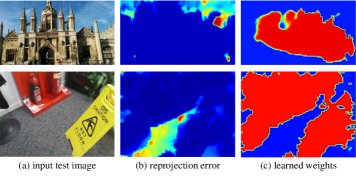
Figure 1: For input images (a), our network firstly regresses their scene coordinates, then predicts correspondence-wise weights (c). With these weights, we can use all 2D-3D correspondences for end-to-end differentiable least squares pose estimation. We use re-projeciton errors (b) to illustrate scene coordinate quality. Our weights select high-quality scene coordinates. A higher color temperature represents a higher value.

In order to get the best of both worlds, we develop a new feed-forward method based upon the state-of-the-art (SOTA) pipeline DSAC* [7], thus enjoying the strong representation power of scene coordinates. We propose an alternative option to RANSAC that exploits all 3D scene coordinate estimates for weighted least squares pose regression (SC-wLS). The key to SC-wLS is a weight network that treats 2D-3D correspondences as 5D point clouds and learns weights that capture geometric patterns in this 5D space, with only pose supervision. Our learned weights can be used to interpret how much each scene coordinate contributes to the least squares solver.

Our SC-wLS estimates poses using only tensor operators on GPUs, which is similar to APR methods due to the feed-forward nature but out-performs APR methods due to the usage of scene coordinates. Furthermore, we show that a self-supervised test-time adaptation step that updates the weight network can lead to further performance improvements. This is potentially useful in scenarios like a robot vacuum adapts to specific rooms during standby time. Although we focus on comparisons with APR methods, we also equip SC-wLS with the LM-Refine post-processing module provided in DSAC* [7] to explore the limits of SC-wLS, and show that it out-performs SOTA on the outdoor dataset Cambridge.

Our major contributions can be summarized as follows: (1) We propose a new feed-forward camera re-localization method, termed SC-wLS, that learns interpretable scene coordinate quality weights (as in Fig. 1) for weighted least squares pose estimation, with only pose supervision. (2) Our method combines the advantages of two paradigms. It exploits learnt 2D-3D correspondences while still allows efficient end-to-end training and feed-forward inference in a principled manner. As a result, we achieve significantly better results than APR methods. (3) Our SC-wLS formulation allows test-time adaptation via self-supervised fine-tuning of the weight network with the photometric loss.

2 Related works

Camera re-localization. In the following, we discuss camera re-localization methods from the perspective of map representation.

Representing image databases with global descriptors like thumbnails [16], BoW [39], or learned features [1] is a natural choice for camera re-localization. By retrieving poses of similar images, localization can be done in the extremely large scale [16, 34]. Meanwhile, CNN-based absolute pose regression methods [22, 42, 8, 49] belong to this category, since their final-layer embeddings are also learned global descriptors. They regress camera poses from single images in an end-to-end manner, and recent work primarily focuses on sequential inputs [48] and network structure enhancement [49, 37, 13]. Although the accuracies of this line of methods are generally low due to intrinsic limitations [33], they are usually compact and fast, enabling pose estimation in a single feed-forward pass.

Maps can also be represented by 3D point cloud [46] with associated 2D descriptors [26] via SfM tools [35]. Given a query image, feature matching establishes sparse 2D-3D correspondences and yields very accurate camera poses with RANSAC-PnP pose optimization [53, 32]. The success of these methods heavily depends on the discriminativeness of features and the robustness of matching strategies. Inspired by feature based pipelines, scene coordinate regression learns a 2D-3D correspondence for each pixel, instead of using feature extraction and matching separately. The map is implicitly encoded into network parameters. [27] demonstrates impressive localization performance using stereo initialization and sequence input. Recently, [2] shows that the algorithm used to create pseudo ground truth has a significant impact on the relative ranking of above methods.

Apart from random forest based methods using RGB-D inputs [38, 40, 28], scene coordinate regression on RGB images is seeing steady progress [4, 5, 6, 7, 56]. This line of work lays the foundation for our research. In this scheme, predicted scene coordinates are noisy due to single-view ambiguity and domain gap during inference. As such, [4, 5] use RANSAC and non-linear optimization to deal with outliers, and NG-RANSAC [6] learns correspondence-wise weights to guide RANSAC sampling. [6] conditions weights on RGB images, whose statistics is often influenced by factors like lighting, weather or even exposure time. Object pose and room layout estimation [23, 55, 17, 18, 54, 50] can also be addressed with similar representations [3, 44].

Differentiable optimization. To enhance their compatibility with deep neural networks and learn result-oriented feature representation, some recent works focus on re-formulating geometric optimization techniques into an end-to-end trainable fashion, for various 3D vision tasks. [20] proposes several standard differentiable optimization layers. [51, 30] propose to estimate fundamental/essential matrix via solving weighted least squares problems with spectral layers. [12] further shows that the eigen-value switching problem when solving least squares can be avoided by minimizing linear system residuals. [14] develops generic black-box differentiable optimization techniques with implicit declarative nodes.

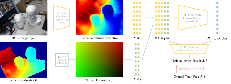
Figure 2: The overview of SC-wLS. Firstly, a fully convolutional network (A) regresses pixel-wise scene coordinates from an input RGB image. Scene coordinate predictions are flattened to the shape of $N\times 3$, with $N$ being pixel count. We concatenate it with normalized $N\times 2$ 2D pixel coordinates, forming $N\times 5$ correspondence inputs. The correspondences are fed into the weight learning network (B), producing $N\times 1$ weights indicating scene coordinate quality. The architecture of B is an order-aware filtering network [52] with graph attention modules [31]. Thirdly, correspondences and weights are sent into a differentiable weighted least squares layer (C), directly outputing camera poses. The scene coordinate ground truth is not used during training.

3 Method

Given an RGB image $I$, we aim to find an estimate of the absolute camera pose consisting of a 3D translation and a 3D rotation, in the world coordinate system. Towards this goal, we exploit the scene coordinate representation. Specifically, for each pixel $i$ with position $\mathbf{p}_{i}$ in an image, we predict the corresponding 3D scene coordinate $\mathbf{s}_{i}$. As illustrated in Fig. 2, we propose an end-to-end trainable deep network that directly calculates global camera poses via weighted least squares. The method is named as SC-wLS. Fig. 2-A is a standard fully convolutional network for scene coordinate regression, as used in former works [7]. Our innovation lies in Fig. 2-B/C, as elaborated below.

3.1 Formulation

Given learned 3D scene coordinates and corresponding 2D pixel positions, our goal is to determine the absolute poses of calibrated images taking all correspondences into account. This would inevitably include outliers, and we need to give them proper weights. Ideally, if all outliers are rejected by zero weights, calculating the absolute pose can be formulated as a linear least squares problem. Inspired by [51] (which solves an essential matrix problem instead), we use all of the $N$ 2D-3D correspondences as input and predict $N$ respective weights $\mathbf{w}_{i}$ using a neural network (Fig. 2-B). $\mathbf{w}_{i}$ indicates the uncertainty of each scene coordinate prediction. As such the ideal least squares problem is turned into a weighted version for pose recovery.

Specifically, the input correspondence $\mathbf{c}_{i}$ to Fig. 2-B is

$$\mathbf{c}_{i}=[x_{i},y_{i},z_{i},u_{i},v_{i}]$$ (1)

where $x_{i},y_{i},z_{i}$ are the three components of the scene coordinate $\mathbf{s}_{i}$, and $u_{i}$, $v_{i}$ denote the corresponding pixel position. $u_{i}$, $v_{i}$ are generated by normalizing $\mathbf{p}_{i}$ with the known camera intrinsic matrix. The absolute pose is written as a transformation matrix $\mathbf{T}\in\mathbb{R}^{3\times 4}$. It projects scene coordinates to the camera plane as below:

$$\begin{bmatrix}u_{i}\\ v_{i}\\ 1\end{bmatrix}\!{=}\mathbf{T}\begin{bmatrix}x_{i}\\ y_{i}\\ z_{i}\\ 1\end{bmatrix}\!{=}\!\begin{bmatrix}p_{1}&p_{2}&p_{3}&p_{4}\\ p_{5}&p_{6}&p_{7}&p_{8}\\ p_{9}&p_{10}&p_{11}&p_{12}\\ \end{bmatrix}\begin{bmatrix}x_{i}\\ y_{i}\\ z_{i}\\ 1\end{bmatrix}\;$$ (2)

When $N>6$, the transformation matrix $\mathbf{T}$ can be recovered by Direct Linear Transform (DLT) [15], which converts Eq. 2 into a linear system:

$$\mathbf{X}\rm Vec(\mathbf{T})=0$$ (3)

$\rm Vec(\mathbf{T})$ is the vectorized $\mathbf{T}$. $\mathbf{X}$ is a $\mathbb{R}^{2N\times 12}$ matrix whose $2i-1$ and $2i$ rows $\mathbf{X}^{(2i{-}1)}$ , $\mathbf{X}^{(2i)}$ are as follows:

$$\begin{bmatrix}x_{i},y_{i},z_{i},1,\;0,\;0,\;0,\;0,-u_{i}x_{i},-u_{i}y_{i},-u_{i}z_{i},-u_{i}\\ 0,\;0,\;0,\;0,\;x_{i},y_{i},z_{i},1,-v_{i}x_{i},-v_{i}y_{i},-v_{i}z_{i},-v_{i}\end{bmatrix}$$ (4)

As such, pose estimation is formulated as a least squares problem. $\rm Vec(\mathbf{T})$ can be recovered by finding the eigenvector associated to the smallest eigenvalue of $\mathbf{X}^{\top}\mathbf{X}$.

Note that in SC-wLS, each correspondence contributes differently according to $\mathbf{w}_{i}$, so $\mathbf{X}^{\top}\mathbf{X}$ can be rewritten as $\mathbf{X}^{\top}\rm diag(\mathbf{w})\mathbf{X}$ and $\rm Vec(\mathbf{T})$ still corresponds to its smallest eigenvector. As the rotation matrix $\mathbf{R}$ needs to be orthogonal and has determinant $1$, we further refine the DLT results by the generalized Procrustes algorithm [36], which is also differentiable. More details about this post-processing step can be found in the supplementary material.

3.2 Network design

Then we describe the architecture of Fig. 2-B. We treat the set of correspondences $\{\mathbf{c}_{i}\}$ as unordered 5-dimensional point clouds and resort to a PointNet-like architecture [52] dubbed OANet. This hierarchical network design consists of multiple components including DiffPool layers, Order-Aware filtering blocks and DiffUnpool layers. It can guarantee the permutation-invariant property of input correspondences. Our improved version enhances the Order-Aware filtering block with self-attention.

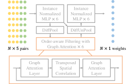
Figure 3: The architecture of Fig. 2-B, which is inherited from OANet [52]. Here we use two self-attention graph layers from [31] while in the original OANet they are instance normazlied MLPs.

The network is illustrated in Fig. 3. Specifically speaking, the DiffPool layer firstly clusters inputs into a particularly learned canonical order. Then the clusters are spatially correlated to retrieve the permutation-invariant context and finally recovered back to original size through the DiffUnpool operator. Inspired by the success of transformer [41] and its extension in 3D vision [31], we propose to introduce the self-attention mechanism into OANet to better reason about the underlying relationship between correspondences. As shown in Fig. 3, there are two instance normalized MLP modules before and after the transposed spatial correlation module, in original OANet. We replace them with attention-based message passing modules, which can exploit the spatial and contextual information simultaneously.

The clusters can be regarded as nodes $\mathcal{V}=\{v_{i}\}$ in a graph $\mathcal{G}$ and the edges $\mathcal{E}=\{e_{i}\}$ are constructed between every two nodes. Since the number of clusters is significantly less than that of original inputs, calculating self-attention on these fully connected weighted edges would be tractable, in terms of computation speed and memory usage. Let ${}^{(\rm in)}\mathbf{f}_{i}$ be the intermediate representation for node $v_{i}$ at input, and the self-attention operator can be described as:

$${}^{(\rm out)}\mathbf{f}_{i}={}^{(\rm in)}\mathbf{f}_{i}+\text{MLP}\left(\left[{}^{(\rm in)}\mathbf{f}_{i}\,||\,\mathbf{m}_{\mathcal{E}\rightarrow i}\right]\right),$$ (5)

where $\mathbf{m}_{\mathcal{E}\rightarrow i}$ is the message aggregated from all other nodes $\{j:(i,j)\in\mathcal{E}\}$ using self-attention described in [31], and $[\cdot\,||\,\cdot]$ denotes concatenation.

Finally, we apply two sequential activation functions (a ReLU followed by a Tanh) upon the outputs of Fig. 3 to get the weights $\mathbf{w}_{i}$ in the range $[0,1)$, for indoor scenes. We use the log-sigmoid activation for outdoor environments following [6], for more stable gradient back-propagation.

3.3 Loss functions

Generating ground-truth scene coordinates for supervision is time-consuming for real-world applications. To this end, our whole framework is solely supervised by ground-truth poses without accessing any 3D models. Successfully training the network with only pose supervision requires three stages using different loss functions. Before describing the training protocol, we first define losses here.

Re-projection loss is defined as follows:

$$r_{i}=||\mathbf{K}\mathbf{T}^{-1}\mathbf{s}_{i}-\mathbf{p}_{i}||_{2},$$ (6)

$$\mathcal{L}_{p}^{(i)}=\begin{cases}r_{i}&\text{if }\mathbf{s}_{i}\in\rm V\\ ||\bar{\mathbf{s}}_{i}-\mathbf{s}_{i}||_{1}&\text{otherwise}.\end{cases}$$ (7)

$$\mathcal{L}_{p}=\frac{1}{N}\sum_{i=1}^{N}\mathcal{L}_{p}^{(i)}$$ (8)

$\mathbf{K}$ is the known camera intrinsic matrix, and $\rm V$ is a set of predicted $\mathbf{s}_{i}$ that meet some specific validity constraints following DSAC* [7]. If $\mathbf{s}_{i}\in\rm V$, we use the re-projection error $r_{i}$ in Eq. 6. Otherwise, we generate a heuristic $\bar{\mathbf{s}}_{i}$ assuming a depth of $10$ meters. This hyper-parameter is inherited from [7].

Classification loss $\mathcal{L}_{c}$ Without knowing the ground truth for scene coordinate quality weights, we utilize the re-projection error $r_{i}$ for weak supervision:

$$l_{i}=\begin{cases}0,&\text{if $r_{i}>\tau$}\\ 1,&\text{otherwise}\end{cases}$$ (9)

$$\mathcal{L}_{c}=\frac{1}{N}\sum_{i=1}^{N}H\left(l_{i},\mathbf{w}_{i}\right)\;,$$ (10)

where $H$ is the binary cross-entropy function. $\tau$ is empirically set to $1$ pixel to reject outliers. Ablation studies about $\mathcal{L}_{c}$ can be found in the supplementary.

Regression loss $\mathcal{L}_{r}$ Since our SC-wLS method is fully differentiable using the eigen-decomposition (ED) technique [20], imposing $L_{2}$ or other losses on the transform matrix $\mathbf{T}$ is straighfoward. However, as illustrated in [12], the eigen-decomposition operations would result in gradient instabilities due to the eigen vector switching phenomenon. Thus we utilize the eigen-decomposition free loss [12] to constrain the pose output, which avoids explicitly performing ED so as to guarantee convergence:

$$\mathcal{L}_{r}=\mathbf{t}^{\top}\mathbf{X}^{\top}\rm diag(\mathbf{w})\mathbf{X}\mathbf{t}\ +\alpha e^{-\beta tr(\mathbf{\bar{X}}^{\top}\rm diag(\mathbf{w})\mathbf{\bar{X}})}$$ (11)

where $\mathbf{t}$ is the flattened ground-truth pose, $\mathbf{\bar{X}}{=}\mathbf{X}(\mathbf{I}-\mathbf{t}\mathbf{t}^{\top})$, $\alpha$ and $\beta$ are positive scalars. Two terms in Eq. 11 serve as different roles. The former tends to minimize the error of pose estimation while the latter tries to alleviate the impact of null space. The trace value in the second term can change up to thousands for different batches, thus the hyper-parameter $\beta$ should be set to balance this effect.

3.4 Training protocol

We propose a three-stage protocol with different objective functions to train our network Fig. 2. Note that ground truth poses are known in all three stages.

Scene coordinate initialization. Firstly, we train our scene coordinate regression network (Fig. 2-A) by optimizing the re-projection error $\mathcal{L}_{p}$ in Eq. 8, using ground truth poses. This step gives us reasonable initial scene coordinates, which are critical for the convergence of $\mathcal{L}_{c}$ and $\mathcal{L}_{r}$.

Weight initialization. Secondly, we exploit $\mathcal{L}=\mathcal{L}_{c}+\gamma\mathcal{L}_{r}$ to train Fig. 2-B, where $\gamma$ is a balancing weight. The classification loss $\mathcal{L}_{c}$ is used to reject outliers. The regression loss $\mathcal{L}_{r}$ is used to constrain poses, making a compromise between the accuracy of estimated weights and how much information is reserved in the null-space. $\mathcal{L}_{c}$ is important to the stable convergence of this stage.

End-to-end optimization. As mentioned above, our whole pipeline is fully differentiable thus capable of learning both scene coordinates and quality weights, directly from ground truth poses. In the third stage, we train both the scene coordinate network (Fig. 2-A) and quality weight network (Fig. 2-B) using $\mathcal{L}$, forcing both of them to learn task-oriented feature representations.

3.5 Optional RANSAC-like post-processing

The SC-wLS method allows us to directly calculate camera poses with DLT. Although we focus on feed-forward settings, it is still possible to use RANSAC-like post-processing for better results. Specifically, we adopt the Levenberg-Marquardt solver developed by [7] to post-process DLT poses as an optional step (shortened as LM-Refine). It brings a boost of localization accuracy.

Specifically, this LM-Refine module is an iterative procedure. It first determines a set of inlier correspondences according to current pose estimate then optimizes poses using the Levenberg–Marquardt algorithm over the inlier set w.r.t. re-projection errors in Eq. 6. This process stops when the number of inlier set converges or until the maximum iteration, which we set to 100 following [7].

3.6 Self-supervised adaptation

At test time, we do not have ground truth pose for supervision. However, if the test data is given in the form of image sequences, we could use the photometric loss in co-visible RGB images to supervise our quality weight network Fig. 2-B. We sample two consecutive images $\emph{I}^{s}$ and $\emph{I}^{t}$ from the test set and synthesize $\tilde{\emph{I}^{t}}$ by warping $\emph{I}^{s}$ to $\emph{I}^{t}$, similar to self-supervised visual odometry methods [57, 25]:

$$p^{t}\sim\mathbf{K}\mathbf{T}_{t}^{-1}\mathbf{s}^{s}$$ (12)

$$\mathcal{L}_{\rm ph}=\sum_{p}||\emph{I}^{t}(p)-\tilde{\emph{I}^{t}}(p)||_{1}+\mathcal{L}_{\rm SSIM}$$ (13)

where $p$ indexes over pixel coordinates, and $\tilde{\emph{I}^{t}}$ is the source view $\emph{I}^{s}$ warped to the target frame based on the predicted global scene coordinates $\mathbf{s}^{s}$. $\mathcal{L}_{\rm SSIM}$ is the structured similarity loss [58] imposed on $\emph{I}^{t}(p)$ and $\tilde{\emph{I}^{t}}(p)$.

Scene coordinates can be trained by $\mathcal{L}_{\rm ph}$ via two gradient paths: (1) the sampling location generation process in Eq. 12. (2) the absolute pose $\mathbf{T}_{t}$ which is calculated by DLT on scene coordinates. However, we observe that fine-tuning scene coordinates with $\mathcal{L}_{\rm ph}$ results in divergence. To this end, we detach scene coordinates from computation graphs and only fine-tune the quality weight net (Fig. 2-B) with self supervision. As will be shown later in experiments, this practice greatly improves re-localization performance. A detailed illustration of this adaptation scheme is provided in the supplementary material.

To clarity, our test-time adaptation experiments exploit all frames in the test set for self-supervision. An ideal online formulation would only use frames before the one of interest. The current offline version can be useful in scenarios like robot vacuums adapts to specific rooms during standby time.

Table 1: Median errors on the 7Scenes dataset [38], with translational and rotational errors measured in $m$ and ^∘. Our results are evaluated directly using weighted DLT, without the (optional) LM-Refine step (Section 3.5) and self-supervised adaptation step (Section 3.6). We compare with methods that directly predict poses with neural networks. Ours ($dlt$) and Ours ($dlt$+$e2e$) show results evaluated w/o and w/ the third stage mentioned in Section 3.4. Our results are significantly better.

Methods	Chess	Fire	Heads	Office	Pumpkin	Kitchen	Stairs
PoseNet17 [21]	0.13/4.5	0.27/11.3	0.17/13.0	0.19/5.6	0.26/4.8	0.23/5.4	0.35/12.4
LSTM-Pose [42]	0.24/5.8	0.34/11.9	0.21/13.7	0.30/8.1	0.33/7.0	0.37/8.8	0.40/13.7
BranchNet [47]	0.18/5.2	0.34/9.0	0.20/14.2	0.30/7.1	0.27/5.1	0.33/7.4	0.38/10.3
GPoseNet [9]	0.20/7.1	0.38/12.3	0.21/13.8	0.28/8.8	0.37/6.9	0.35/8.2	0.37/12.5
MLFBPPose [45]	0.12/5.8	0.26/12.0	0.14/13.5	0.18/8.2	0.21/7.1	0.22/8.1	0.38/10.3
AttLoc [43]	0.10/4.1	0.25/11.4	0.16/11.8	0.17/5.3	0.21/4.4	0.23/5.4	0.26/10.5
MapNet [8]	0.08/3.3	0.27/11.7	0.18/13.3	0.17/5.2	0.22/4.0	0.23/4.9	0.30/12.1
LsG [48]	0.09/3.3	0.26/10.9	0.17/12.7	0.18/5.5	0.20/3.7	0.23/4.9	0.23/11.3
GL-Net [49]	0.08/2.8	0.26/8.9	0.17/11.4	0.18/5.1	0.15/2.8	0.25/4.5	0.23/8.8
MS-Transformer [37]	0.11/4.7	0.24/9.6	0.14/12.2	0.17/5.7	0.18/4.4	0.17/5.9	0.26/8.5
Ours ($dlt$)	0.029/0.78	0.051/1.04	0.026/2.00	0.063/0.93	0.084/1.28	0.099/1.60	0.179/3.61
Ours ($dlt$+$e2e$)	0.029/0.76	0.048/1.09	0.027/1.92	0.055/0.86	0.077/1.27	0.091/1.43	0.123/2.80

4 Experiments

4.1 Experiment setting

Datasets. We evaluate our SC-wLS framework for camera re-localization from single RGB images, on both indoor and outdoor scenes. Following [7], we choose the publicly available indoor 7Scenes dataset [38] and outdoor Cambridge dataset [22], which have different scales, appearance and motion patterns. These two datasets have fairly different distributions of scene coordinates. We would show later that, in both cases, SC-wLS successfully predicts interpretable scene coordinate weights for feed-forward camera re-localization.

Table 2: Median errors on the Cambridge dataset [22], with translational and rotational errors measured in $m$ and ^∘. Settings are the same as Table 1. Our results are significantly better than other methods. Note that GL-Net uses a sequence as input.

Methods	Greatcourt	King’s College	Shop Facade	Old Hospital	Church
ADPoseNet [19]	N/A	1.30/1.7	1.22/6.7	N/A	2.28/4.8
PoseNet17 [21]	7.00/3.7	0.99/1.1	1.05/4.0	2.17/2.9	1.49/3.4
GPoseNet [9]	N/A	1.61/2.3	1.14/5.7	2.62/3.9	2.93/6.5
MLFBPPose [45]	N/A	0.76/1.7	0.75/5.1	1.99/2.9	1.29/5.0
LSTM-Pose [42]	N/A	0.99/3.7	1.18/7.4	1.51/4.3	1.52/6.7
SVS-Pose [29]	N/A	1.06/2.8	0.63/5.7	1.50/4.0	2.11/8.1
MapNet [8]	N/A	1.07/1.9	1.49/4.2	1.94/3.9	2.00/4.5
GL-Net [49]	6.67/2.8	0.59/0.7	0.50/2.9	1.88/2.8	1.90/3.3
MS-Transformer [37]	N/A	0.83/1.5	0.86/3.1	1.81/2.4	1.62/4.0
Ours ($dlt$)	1.81/1.2	0.22/0.9	0.15/1.1	0.46/1.9	0.50/1.5
Ours ($dlt$+$e2e$)	1.64/0.9	0.14/0.6	0.11/0.7	0.42/1.7	0.39/1.3

Implementation. The input images are proportionally resized so that the heights are 480 pixels. We randomly zoom and rotate images for data augmentation following [7]. As mentioned in Sec. 3.3, $\alpha$ and $\beta$ in Eq. 11 are sensitive to specific scenes. We set them to 5 and 1e-4 for indoor 7Scenes while 5 and 1e-6 for outdoor Cambridge, respectively. The balancing hyper-parameter $\gamma$ is set to 5 empirically. We train our model on one nVIDIA GeForce RTX 3090 GPU. The ADAM optimizer with initial learning rate 1e-4 is utilized in the first two training stages and the learning rate is set to 1e-5 in the end-to-end training stage. The batch size is set to 1 as [7]. The scene coordinate regression network architecture for 7Scenes is adopted from [7]. As for Cambridge, we add residual connections to the early layers of this network. Architecture details can be found in the supplementary material.

4.2 Feed-forward Re-localization

An intriguing property of the proposed SC-wLS method is that we can re-localize a camera directly using weighted least squares. This inference scheme seamlessly blends into the forward pass of a neural network. So we firstly compare with other APR re-localization methods that predict camera poses directly with a neural network during inference. Quantitative results on 7Scenes and Cambridge are summarized in Table 1 and Table 2, respectively.

Table 3: Results on the 7Scenes dataset [38] and the Cambrdige dataset [22], with translational and rotational errors measured in $m$ and ^∘. Here $ref$ means LM-Refine. Note DSAC* [7] w/o model and NG-RANSAC [6] also use the LM pose refinement process. Note that with ref used, our method loses the feed-forward nature. NG-RANSAC w/o model${\dagger}$ is retrained using DSAC* RGB initialization.

7Scenes	Chess	Fire	Heads	Office	Pumpkin	Kitchen	Stairs
DSAC* [7] w/o model	0.019/1.11	0.019/1.24	0.011/1.82	0.026/1.18	0.042/1.42	0.030/1.70	0.041/1.42
Ours ($dlt$+$ref$)	0.018/0.63	0.026/0.84	0.015/0.87	0.038/0.85	0.045/1.05	0.051/1.17	0.067/1.93
Ours ($dlt$+$e2e$+$ref$)	0.019/0.62	0.025/0.88	0.014/0.90	0.035/0.78	0.051/1.07	0.054/1.15	0.058/1.57
Cambridge		Greatcourt	King’s College	Shop Facade	Old Hospital	Church
DSAC* [7] w/o model		0.34/0.2	0.18/0.3	0.05/1.3	0.21/0.4	0.15/0.6
NG-RANSAC [6]		0.35/0.2	0.13/0.2	0.06/0.3	0.22/0.4	0.10/0.3
NG-RANSAC w/o model†		0.31/0.2	0.15/0.3	0.05/0.3	0.20/0.4	0.12/0.4
Ours ($dlt$+$ref$)		0.32/0.2	0.09/0.3	0.04/0.3	0.12/0.4	0.12/0.4
Ours ($dlt$+$e2e$+$ref$)		0.29/0.2	0.08/0.2	0.04/0.3	0.11/0.4	0.09/0.3

As for former arts, we distinguish between two cases: single frame based and sequence based. They are separated by a line in Table 1 and Table 2. As for our results, we report under two settings: Ours ($dlt$) and Ours ($dlt$+$e2e$). Ours ($dlt$+$e2e$) means all three training stages are finished (see Section 3.4), while Ours ($dlt$) means only the first two stages are used.

On 7Scenes, it is clear that our SC-wLS method out-performs APR camera re-localization methods by significant margins. Note we only take a single image as input, and still achieve much lower errors than sequence-based methods like GLNet [49]. On Cambrige, SC-wLS also reports significantly better results including the Greatcourt scene. Note that this scene has extreme illumination conditions and most former solutions do not even work.

Table 4: Recalls (%) on the 7Scenes dataset [38] and the Cambrdige dataset [22].

7Scenes	Chess	Fire	Heads	Office	Pumpkin	Kitchen	Stairs	Avg
DSAC* [7] w/o model	96.7	92.9	98.2	87.1	60.7	65.3	64.1	80.7
Active Search [32]	86.4	86.3	95.7	65.6	34.1	45.1	67.8	68.7
Ours ($dlt$+$e2e$+$ref$)	93.7	82.2	65.7	73.5	49.6	45.3	43.0	64.7
Ours ($dlt$+$e2e$+$dsac*$)	96.8	97.4	94.3	88.6	62.4	65.5	55.3	80.0
Cambridge		Great	King’s	Shop	Old	Church	Avg
		Court	College	Facade	Hospital
DSAC* [7] w/o model		62.9	80.8	86.4	55.5	88.9	74.9
NG-RANSAC w/o model†		67.6	81.9	88.3	56.0	93.8	77.5
Ours ($dlt$+$e2e$+$ref$)		73.3	97.3	90.3	75.3	82.2	83.7
Ours ($dlt$+$e2e$+$dsac*$)		74.3	87.2	87.4	53.8	99.1	80.4

Why SC-wLS performs much better than former APR methods that directly predict poses without RANSAC? Because they are black boxes, failing to model explicit geometric relationships. These black-box methods suffer from hard memorization and dataset bias. By contrast, our formulation is based upon 2D-3D correspondences, while still allowing feed-forward inference.

Lastly, Ours ($dlt$+$e2e$) shows lower errors than Ours ($dlt$) in most scenes, validating the effectiveness of jointly fine-tuning Fig. 2-A and Fig. 2-B.

4.3 Optional LM-Refine

The most interesting part about SC-wLS is the strong re-localization ability without using iterative pose estimation methods like RANSAC or LM-Refine. However, although optional, incorporating such methods does lead to lower errors. We report quantitative comparisons in Table 3. We compare with the best published method DSAC* in the ’w/o model’ setting for two reasons: 1) Our training protocol does not involve any usage of 3D models; 2) DSAC* also uses LM-Refine as a post-processing step. Note LM-Refine needs pose initialization, so we use DLT results as initial poses. Similar to above experiments, Ours ($dlt$+$e2e$+$ref$) means all three training stages are used. For Cambridge, we also compare to NG-RANSAC [6], which predicts weights from RGB images.

On the Cambridge dataset, SC-wLS outperforms state-of-the-art methods. On the Old Hospital scene, we reduce the translational error from 0.21m to 0.11m, which is a 47.6% improvement. Meanwhile, Ours ($dlt$+$e2e$+$ref$) consistently achieves lower errors than Ours ($dlt$+$ref$), showing the benefits of end-to-end joint learning. On the 7Scenes dataset, our results under-perform DSAC* and the third training stage does not bring clear margins.

Table 5: Results on the 7Scenes dataset [38] and the Cambrdige dataset [22], with translational and rotational errors measured in $m$ and ^∘. Here $self$ means self-supervised adaptation. Note these results are evaluated without LM-Refine.

7Scenes	Chess	Fire	Heads	Office	Pumpkin	Kitchen	Stairs
Ours ($dlt$+$e2e$)	0.029/0.76	0.048/1.09	0.027/1.92	0.055/0.86	0.077/1.27	0.091/1.43	0.123/2.80
Ours ($dlt$+$e2e$+$self$)	0.021/0.64	0.023/0.80	0.013/0.79	0.037/0.76	0.048/1.06	0.051/1.08	0.055/1.48
Cambridge		Greatcourt	King’s College	Shop Facade	Old Hospital	Church
Ours ($dlt$+$e2e$)		1.64/0.9	0.14/0.6	0.11/0.7	0.42/1.7	0.39/1.3
Ours ($dlt$+$e2e$+$self$)		0.94/0.5	0.11/0.3	0.05/0.4	0.18/0.7	0.17/0.8

We also report average recalls with pose error below 5cm, 5deg (7Scenes) and translation error below 0.5% of the scene size (Cambridge) in Table 4. It is demonstrated that the recall value of Ours ($dlt$+$e2e$+$ref$) under-performs SOTA on 7Scenes, which is consistent with the median error results. We also evaluate DSAC*’s exact post-processing, denoted as Our ($dlt$+$e2e$+$dsac*$). The difference is that for Ours ($dlt$+$e2e$+$ref$) we use DLT results for LM-Refine initialization and for Ours ($dlt$+$e2e$+$dsac*$) we use RANSAC for LM-Refine initialization. It is shown that using DSAC*’s exact post-processing can compensate for the performance gap on 7Scenes.

4.4 Self-supervised Adaptation

We show the effectiveness of self-supervised weight network adaptation during test time, which is a potentially useful new feature of SC-wLS (Section 3.6). Results are summarized in Table 5, which is evaluated under the weighted DLT setting (same as Section 4.2). Obviously, for all sequences in 7Scenes and Cambridge, Ours ($dlt$+$e2e$+$self$) outperforms Ours ($dlt$+$e2e$) by clear margins. On Stairs and Old Hospital, translational and rotational error reductions are both over 50%. In these experiments, self-supervised adaptation runs for about 600k iterations. Usually, this adaptation process converges to a reasonably good state, within only 150k iterations. More detailed experiments are in the supplementary.

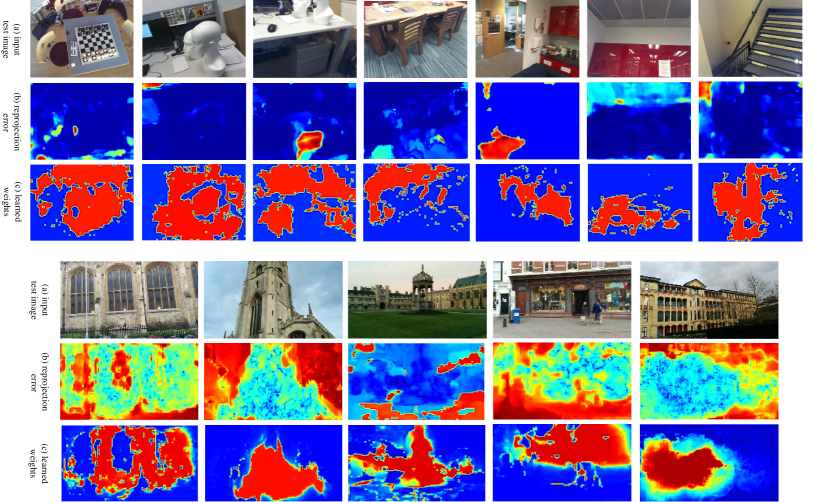
Figure 4: Visualizations on 7Scenes and Cambridge test sets, demonstrating that our network learns interpretable scene coordinate weights consistent with re-projection errors, by solely considering the intrinsic structure of input 2D-3D correspondences. A higher color temperature represents a higher value.

4.5 Visualization

Firstly, we demonstrate more learnt weights on the test sets of 7Scenes and Cambridge, in Fig. 4. The heatmaps for reprojection error and learnt weight are highly correlated. Pixels with low quality weights usually have high reprojection errors and occur in sky or uniformly textured regions.

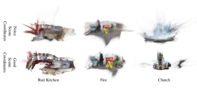
Figure 5: Map visualization on 7Scenes and Cambridge. More comparisons are provided in the supplementary material.

Secondly, We show learnt 3D maps with and without quality filtering, in Fig. 5. Since scene coordinates are predicted in the world frame, we directly show the point clouds generated by aggregating scene coordinate predictions on test frames. It is shown that only predicting scene coordinates results in noisy point clouds, especially in outdoor scenes where scene coordinate predictions on sky regions are only meaningful in term of their 2D projections. We show good scene coordinates by filtering out samples with a quality weight lower than 0.9.

4.6 Training and Inference Efficiency

As shown in Table 6, our method, as a feed-forward (fw) one, is faster than the well-engineered iterative (iter) method DSAC* and the transformer-based method MS-Transformer [37]. We could make a tradeoff using OANet w/o attention for even faster speed. Thus it’s reasonable to compare our feed-forward method with APR methods. We also evaluate end-to-end training efficiency. When training 5 network instances for 5 different scenes on 5 GPUs, the average time of ours stays unchanged, while that of DSAC* increases due to limited CPU computation/scheduling capacity. We believe large-scale training of many re-localization network instances on the cloud is an industry demand.

Table 6: Average end-to-end training and inference time comparisons.

Inference time (ms/frame)								End-to-end training time (s/frame)
Method	AtLoc	MapNet	Ours	Ours	MS-T	DSAC*		Setting	Ours	DSAC*	NG-RANSAC
	[43]	[8]	(OANet)		[37]	[7]				[7]	[6]
Type	fw	fw	fw	fw	fw	iter		1-GPU	0.09	0.20	0.31
Time	6	9	13	19	30	32		5-GPU	0.09	0.85	1.05

5 Conclusions

In this study, we propose a new camera re-localization solution named SC-wLS, which combines the advantages of feed-forward formulations and scene coordinate based methods. It exploits the correspondences between pixel coordinates and learnt 3D scene coordinates, while still allows direct camera re-localization through a single forward pass. This is achieved by a correspondence weight network that finds high-quality scene coordinates, supervised by poses only. Meanwhile, SC-wLS also allows self-supervised test-time adaptation. Extensive evaluations on public benchmarks 7Scenes and Cambridge demonstrate the effectiveness and interpretability of our method. In the feed-forward setting, SC-wLS results are significantly better than APR methods. When coupled with LM-Refine post-processing, our method out-performs SOTA on outdoor scenes and under-performs SOTA on indoor scenes.

Acknowledgement This work was supported by the National Natural Science Foundation of China under Grant 62176010.

References

- [1] Arandjelovic, R., Gronat, P., Torii, A., Pajdla, T., Sivic, J.: Netvlad: Cnn architecture for weakly supervised place recognition. In: Proceedings of the IEEE conference on computer vision and pattern recognition. pp. 5297–5307 (2016)
- [2] Brachmann, E., Humenberger, M., Rother, C., Sattler, T.: On the limits of pseudo ground truth in visual camera re-localisation. In: Proceedings of the IEEE/CVF International Conference on Computer Vision. pp. 6218–6228 (2021)
- [3] Brachmann, E., Krull, A., Michel, F., Gumhold, S., Shotton, J., Rother, C.: Learning 6d object pose estimation using 3d object coordinates. In: European conference on computer vision. pp. 536–551. Springer (2014)
- [4] Brachmann, E., Krull, A., Nowozin, S., Shotton, J., Michel, F., Gumhold, S., Rother, C.: Dsac-differentiable ransac for camera localization. In: CVPR (2017)
- [5] Brachmann, E., Rother, C.: Learning less is more - 6d camera localization via 3d surface regression. CVPR (2018)
- [6] Brachmann, E., Rother, C.: Neural-guided ransac: Learning where to sample model hypotheses. ICCV (2019)
- [7] Brachmann, E., Rother, C.: Visual camera re-localization from rgb and rgb-d images using dsac. IEEE Transactions on Pattern Analysis and Machine Intelligence (2021)
- [8] Brahmbhatt, S., Gu, J., Kim, K., Hays, J., Kautz, J.: Geometry-aware learning of maps for camera localization. In: CVPR (2018)
- [9] Cai, M., Shen, C., Reid, I.: A hybrid probabilistic model for camera relocalization (2019)
- [10] Cao, S., Snavely, N.: Graph-based discriminative learning for location recognition. In: IJCV (2015)
- [11] Choi, S., Kim, T., Yu, W.: Performance evaluation of ransac family. Journal of Computer Vision 24(3), 271–300 (1997)
- [12] Dang, Z., Yi, K.M., Hu, Y., Wang, F., Fua, P., Salzmann, M.: Eigendecomposition-free training of deep networks for linear least-square problems. TPAMI (2020)
- [13] Ding, M., Wang, Z., Sun, J., Shi, J., Luo, P.: Camnet: Coarse-to-fine retrieval for camera re-localization. In: Proceedings of the IEEE/CVF International Conference on Computer Vision. pp. 2871–2880 (2019)
- [14] Gould, S., Hartley, R., Campbell, D.J.: Deep declarative networks. TPAMI (2021)
- [15] Hartley, R., Zisserman, A.: Multiple view geometry in computer vision: N-view geometry (2004)
- [16] Hays, J., Efros, A.A.: Im2gps: estimating geographic information from a single image. In: CVPR (2008)
- [17] Hedau, V., Hoiem, D., Forsyth, D.: Recovering the spatial layout of cluttered rooms. In: 2009 IEEE 12th international conference on computer vision. pp. 1849–1856. IEEE (2009)
- [18] Hirzer, M., Lepetit, V., ROTH, P.: Smart hypothesis generation for efficient and robust room layout estimation. In: Proceedings of the IEEE/CVF winter conference on applications of computer vision. pp. 2912–2920 (2020)
- [19] Huang, Z., Xu, Y., Shi, J., Zhou, X., Bao, H., Zhang, G.: Prior guided dropout for robust visual localization in dynamic environments. In: ICCV (2019)
- [20] Ionescu, C., Vantzos, O., Sminchisescu, C.: Matrix backpropagation for deep networks with structured layers. In: ICCV (2015)
- [21] Kendall, A., Cipolla, R.: Geometric loss functions for camera pose regression with deep learning. In: CVPR (2017)
- [22] Kendall, A., Grimes, M., Cipolla, R.: Posenet: A convolutional network for real-time 6-dof camera relocalization. In: ICCV (2015)
- [23] Lepetit, V., Fua, P., et al.: Monocular model-based 3d tracking of rigid objects: A survey. Foundations and Trends® in Computer Graphics and Vision 1(1), 1–89 (2005)
- [24] Li, S., Xu, C., Xie, M.: A robust o (n) solution to the perspective-n-point problem. IEEE transactions on pattern analysis and machine intelligence 34(7), 1444–1450 (2012)
- [25] Li, S., Wu, X., Cao, Y., Zha, H.: Generalizing to the open world: Deep visual odometry with online adaptation. In: Proceedings of the IEEE/CVF Conference on Computer Vision and Pattern Recognition. pp. 13184–13193 (2021)
- [26] Lowe, D.G.: Distinctive image features from scale-invariant keypoints. IJCV (2004)
- [27] Mair, E., Strobl, K.H., Suppa, M., Burschka, D.: Efficient camera-based pose estimation for real-time applications. In: 2009 IEEE/RSJ International Conference on Intelligent Robots and Systems. pp. 2696–2703. IEEE (2009)
- [28] Meng, L., Tung, F., Little, J.J., Valentin, J., de Silva, C.W.: Exploiting points and lines in regression forests for rgb-d camera relocalization. In: IROS (2018)
- [29] Naseer, T., Burgard, W.: Deep regression for monocular camera-based 6-dof global localization in outdoor environments. In: IROS (2017)
- [30] Ranftl, R., Koltun, V.: Deep fundamental matrix estimation. In: ECCV (2018)
- [31] Sarlin, P.E., DeTone, D., Malisiewicz, T., Rabinovich, A.: Superglue: Learning feature matching with graph neural networks. In: CVPR (2020)
- [32] Sattler, T., Leibe, B., Kobbelt, L.: Efficient & effective prioritized matching for large-scale image-based localization. TPAMI (2016)
- [33] Sattler, T., Zhou, Q., Pollefeys, M., Leal-Taixe, L.: Understanding the limitations of cnn-based absolute camera pose regression. In: CVPR (2019)
- [34] Schindler, G., Brown, M., Szeliski, R.: City-scale location recognition. In: CVPR (2007)
- [35] Schonberger, J.L., Frahm, J.M.: Structure-from-motion revisited. In: Proceedings of the IEEE conference on computer vision and pattern recognition. pp. 4104–4113 (2016)
- [36] Schönemann, P.H.: A generalized solution of the orthogonal procrustes problem. Psychometrika 31(1), 1–10 (1966)
- [37] Shavit, Y., Ferens, R., Keller, Y.: Learning multi-scene absolute pose regression with transformers. In: Proceedings of the IEEE/CVF International Conference on Computer Vision. pp. 2733–2742 (2021)
- [38] Shotton, J., Glocker, B., Zach, C., Izadi, S., Criminisi, A., Fitzgibbon, A.: Scene coordinate regression forests for camera relocalization in rgb-d images. In: CVPR (2013)
- [39] Sivic, J., Zisserman, A.: Video google: A text retrieval approach to object matching in videos. In: ICCV (2003)
- [40] Valentin, J., Nießner, M., Shotton, J., Fitzgibbon, A., Izadi, S., Torr, P.H.: Exploiting uncertainty in regression forests for accurate camera relocalization. In: CVPR (2015)
- [41] Vaswani, A., Shazeer, N., Parmar, N., Uszkoreit, J., Jones, L., Gomez, A.N., Kaiser, L., Polosukhin, I.: Attention is all you need (2017)
- [42] Walch, F., Hazirbas, C., Leal-Taixe, L., Sattler, T., Hilsenbeck, S., Cremers, D.: Image-based localization using lstms for structured feature correlation. In: ICCV (2017)
- [43] Wang, B., Chen, C., Lu, C.X., Zhao, P., Trigoni, N., Markham, A.: Atloc: Attention guided camera localization. In: Proceedings of the AAAI Conference on Artificial Intelligence. vol. 34, pp. 10393–10401 (2020)
- [44] Wang, H., Sridhar, S., Huang, J., Valentin, J., Song, S., Guibas, L.J.: Normalized object coordinate space for category-level 6d object pose and size estimation. In: Proceedings of the IEEE/CVF Conference on Computer Vision and Pattern Recognition. pp. 2642–2651 (2019)
- [45] Wang, X., Wang, X., Wang, C., Bai, X., Wu, J., Hancock, E.R.: Discriminative features matter: Multi-layer bilinear pooling for camera localization. In: BMVC (2019)
- [46] Wu, C.: Towards linear-time incremental structure from motion. In: 3DV (2013)
- [47] Wu, J., Ma, L., Hu, X.: Delving deeper into convolutional neural networks for camera relocalization. In: ICRA (2017)
- [48] Xue, F., Wang, X., Yan, Z., Wang, Q., Wang, J., Zha, H.: Local supports global: Deep camera relocalization with sequence enhancement. In: ICCV (2019)
- [49] Xue, F., Wu, X., Cai, S., Wang, J.: Learning multi-view camera relocalization with graph neural networks. In: 2020 IEEE/CVF Conference on Computer Vision and Pattern Recognition (CVPR). pp. 11372–11381. IEEE (2020)
- [50] Yan, C., Shao, B., Zhao, H., Ning, R., Zhang, Y., Xu, F.: 3d room layout estimation from a single rgb image. IEEE Transactions on Multimedia 22(11), 3014–3024 (2020)
- [51] Yi, K., Trulls, E., Ono, Y., Lepetit, V., Salzmann, M., Fua, P.: Learning to find good correspondences. CVPR (2018)
- [52] Zhang, J., Sun, D., Luo, Z., Yao, A., Zhou, L., Shen, T., Chen, Y., Quan, L., Liao, H.: Learning two-view correspondences and geometry using order-aware network. In: ICCV (2019)
- [53] Zhang, W., Kosecka, J.: Image based localization in urban environments. In: 3DPTV (2006)
- [54] Zhao, H., Lu, M., Yao, A., Guo, Y., Chen, Y., Zhang, L.: Physics inspired optimization on semantic transfer features: An alternative method for room layout estimation. In: Proceedings of the IEEE conference on computer vision and pattern recognition. pp. 10–18 (2017)
- [55] Zhong, L., Zhang, Y., Zhao, H., Chang, A., Xiang, W., Zhang, S., Zhang, L.: Seeing through the occluders: Robust monocular 6-dof object pose tracking via model-guided video object segmentation. IEEE Robotics and Automation Letters 5(4), 5159–5166 (2020)
- [56] Zhou, L., Luo, Z., Shen, T., Zhang, J., Zhen, M., Yao, Y., Fang, T., Quan, L.: Kfnet: Learning temporal camera relocalization using kalman filtering. In: Proceedings of the IEEE/CVF Conference on Computer Vision and Pattern Recognition. pp. 4919–4928 (2020)
- [57] Zhou, T., Brown, M., Snavely, N., Lowe, D.G.: Unsupervised learning of depth and ego-motion from video. In: CVPR (2017)
- [58] Zhou Wang, Bovik, A.C., Sheikh, H.R., Simoncelli, E.P.: Image quality assessment: from error visibility to structural similarity. IEEE Transactions on Image Processing 13(4), 600–612 (2004). https://doi.org/10.1109/TIP.2003.819861