Principal Component Classification

Abstract

We propose to directly compute classification estimates by learning features encoded with their class scores. Our resulting model has a encoder-decoder structure suitable for supervised learning, it is computationally efficient and performs well for classification on several datasets.

Index Terms—  Supervised Learning, PCA, classification

1 Introduction

The choice of data encoding for defining inputs and outputs of machine learning pipelines contributes substantially to their performance. For instance, adding positional encoding in the inputs have shown useful for Convolutional Neural Networks [1] and for Neural radiance Fields [2]. Here, we propose to add vectors of class scores as part of inputs to learn principal components suitable for predicting classification scores. Performance of our proposed frugal model is validated experimentally on datasets wine, australian [3, 4] and MNIST [5] for comparison with metric learning classification [6, 4, 7], and deep learning [5, 8].

2 Principal Component Classification

In supervised learning, we consider available a dataset $\mathcal{B}=\{(\mathbf{x}^{(i)},\mathbf{y}^{(i)})\}_{i=1,\cdots,N}$ of $N$ observations with $\mathbf{x}\in\mathbb{R}^{d_{\mathbf{x}}}$ denoting the feature vector of dimension $d_{\mathbf{x}}$ and $\mathbf{y}\in\mathbb{R}^{n_{c}}$ the indicator class vector where $n_{c}$ is the number of classes. All coordinates of $\mathbf{y}^{(i)}$ are equal to zero at the exception of its coordinate $y_{j}^{(i)}$ that is equal to 1 if $\mathbf{y}^{(i)}$ is indicating that feature vector $\mathbf{x}^{(i)}$ belongs to class $j\in\{1,\cdots,n_{c}\}$.

Principal Component Analysis (PCA) [9] is a standard technique for dimension reduction often used in conjunction with classification techniques [6]. In PCA, the principal components correspond to the eigenvectors of the covariance matrix $\mathrm{\Sigma}$ ranked in descending order of their associated eigenvalues, where $\mathrm{\Sigma}=\frac{1}{N}\mathrm{X}\mathrm{X}^{T}$ and $\mathrm{X}=[\mathbf{x}^{(1)},\cdots,\mathbf{x}^{(N)}]$. These principal components provide a orthonormal basis in the feature space. Retaining only the ones associated with the highest eigenvalues allow to project $\mathbf{x}$ in a very small dimensional eigenspace (data embedding). Such PCA based representation has been used for learning images of objects, to perform detection and registration [10, 11, 12], and has a probabilistic interpretation [13]. PCA for dimensionality reduction of the feature space ignores information from the class labels and we propose next a new data encoding suitable for learning principal components that can be used for classification.

$\alpha=0$
$\alpha=0.9$

Fig. 1: Principal components for classification computed for Dataset MNIST. Effect of $\alpha$ on the first 4 principal components, $\mathbf{u}_{1}$ to $\mathbf{u}_{4}$ (left to right), computed for $\alpha=0$ (top row) and $\alpha=0.9$ (bottom row). For visualisation, eigenvector $\mathbf{u}$ is shown as an image for the first $d_{\mathbf{x}}$ coordinates (in the feature $\mathbf{x}$-space) and as a plot for the remaining of its $n_{c}$ components (in the class $\mathbf{y}$-space). Data is not centred (un-centered PCA) and the first component (left) captures the main deviation of the training dataset from the origin in the $\mathbf{z}$-space.

2.1 Data encoding with Class

Class score vectors have recently been used as node attributes in a graph model for image segmentation [14]. We propose likewise to use that information explicitly by creating a training dataset noted $\mathcal{T}_{\alpha}=\{\mathbf{z}_{\alpha}^{(i)}\}_{i=1,\cdots,N}$ from the dataset $\mathcal{B}$, where each instance $\mathbf{z}^{(i)}_{\alpha}$ concatenates the feature vector $\mathbf{x}^{(i)}$ with its class vector $\mathbf{y}^{(i)}$ as follow:

$$\mathbf{z}_{\alpha}=(1-\alpha)\cdot\begin{pmatrix}\mathbf{x}\\ \mathbf{0}_{\mathbf{y}}\\ \end{pmatrix}+\alpha\cdot\begin{pmatrix}\mathbf{0}_{\mathbf{x}}\\ \mathbf{y}\\ \end{pmatrix}$$ (1)

where $\mathbf{0}_{\mathbf{x}}$ and $\mathbf{0}_{\mathbf{y}}$ are the null vectors of feature space $\mathbb{R}^{d_{\mathbf{x}}}$ and class space $\mathbb{R}^{n_{c}}$ respectively. The scalar $0\leq\alpha\leq 1$ is controlling the weight of the class vector w.r.t. the feature vector, and it is a hyper-parameter in this new framework. The training dataset $\mathcal{T}_{\alpha}$ is stored in a data matrix noted $\mathrm{Z}_{\alpha}=[\mathbf{z}^{(1)}_{\alpha},\cdots,\mathbf{z}^{(N)}_{\alpha}]$. The matrix $\mathrm{Z}_{\alpha}$ concatenates vertically the matrix $\mathrm{X}$ and the matrix $\mathrm{Y}=[\mathbf{y}^{(1)},\cdots,\mathbf{y}^{(N)}]$ as follows:

$$\mathrm{Z}_{\alpha}=\left[\begin{array}[]{c}(1-\alpha)\cdot\mathrm{X}\\ \alpha\cdot\mathrm{Y}\\ \end{array}\right]$$ (2)

We note $d_{\mathbf{z}}=d_{\mathbf{x}}+n_{c}$ the dimension of vectors $\mathbf{z}_{\alpha}$, and the matrix $\mathrm{Z}_{\alpha}$ is of size $d_{\mathbf{z}}\times N$.

2.2 Principal components

The $d_{\mathbf{z}}\times d_{\mathbf{z}}$ covariance matrix $\Sigma_{\alpha}$ is computed as follow:

$$\Sigma_{\alpha}=\frac{1}{N}\ \mathrm{Z}_{\alpha}\mathrm{Z}_{\alpha}^{T}=\mathrm{U}_{\alpha}\Lambda_{\alpha}\mathrm{U}_{\alpha}^{T}$$ (3)

In our experiments, we used Singular Value Decomposition (SVD) to compute the diagonal matrix $\Lambda_{\alpha}$ of eigenvalues $\{\lambda_{i}\}_{i=1,\cdots,d_{\mathbf{z}}}$ of $\Sigma_{\alpha}$ and with the corresponding eigenvectors stored as columns in the matrix $\mathrm{U}_{\alpha}=[\mathbf{u}_{1},\cdots,\mathbf{u}_{d_{\mathbf{z}}}]$. For large training dataset ($N>>0)$, more efficient algorithms alternative to SVD can be used to compute the principal components [15]. Eigenvalues are sorted in decreasing order $\lambda_{1}\geq\lambda_{2}\cdots\geq\lambda_{d_{\mathbf{z}}}\geq 0$ and their associated eigenvectors form a orthonormal basis of the $\mathbf{z}$-space. When $\alpha=0$, only feature vectors appear in the vector $\mathbf{z}_{0}$ corresponding to the standard usage of PCA for dimensionality reduction of the feature space. When $\alpha>0$, the principal components stored in $\mathrm{U}_{\alpha}$ change away from the baseline $\mathrm{U}_{0}$ (e.g. see Fig. 1).

2.3 Encoder & Decoder Model $\mathcal{M}^{n_{e}}_{\alpha}$

Dimensionality reduction is performed by only considering the first $n_{e}$ eigenvectors associated with the $n_{e}$ highest eigenvalues. Noting $\mathrm{U}_{\alpha}^{n_{e}}=[\mathbf{u}_{1},\cdots,\mathbf{u}_{n_{e}}]$, the projection of any vector $\mathbf{z}$ against the first $n_{e}$ eigenvectors is computed as:

$$\mathbf{p}_{\alpha}^{n_{e}}=\left(\mathrm{U}_{\alpha}^{n_{e}}\right)^{T}\mathbf{z}$$ (4)

Projections of the training set $\mathcal{T}_{\alpha}$ can be visualised in the eigenspaces defined by a pair of principal components (cf. Fig. 2) providing renderings similar to TSNE [16].

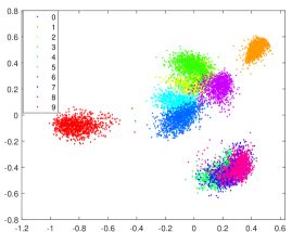
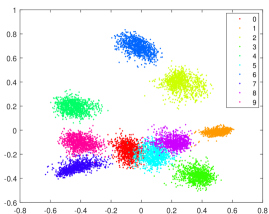
$(\mathbf{u}_{2},\mathbf{u}_{3})$	$(\mathbf{u}_{3},\mathbf{u}_{4})$

Fig. 2: Visualisation of projections. The training set $\mathcal{T}_{\alpha=0.9}$ is projected in the eigenspaces defined by pairs of our learnt principal components for dataset MNIST (shown Fig. 1).

Choosing a small number $n_{e}$ of eigenvectors for projection allows to limit the number of computations, but it also needs to be large enough to capture useful information about the dataset $\mathcal{T}_{\alpha}$. The projection (Eq.4) is a linear encoder of $\mathbf{z}$ which can be decoded as follows:

$$\hat{\mathbf{z}}=\mathrm{U}_{\alpha}^{n_{e}}\mathbf{p}_{\alpha}^{n_{e}}=\mathrm{U}_{\alpha}^{n_{e}}\left(\mathrm{U}_{\alpha}^{n_{e}}\right)^{T}\mathbf{z}$$ (5)

Our model $\mathcal{M}^{n_{e}}_{\alpha}$ is now explicitly defined (Eq. (5)) for transforming any input $\mathbf{z}$ for transformation into an output $\hat{\mathbf{z}}$, using the learnt parameters (matrix $\mathrm{U}^{n_{e}}_{\alpha}$) for the chosen hyper-parameters $\alpha$ and $n_{e}$ (cf. Fig. 3).

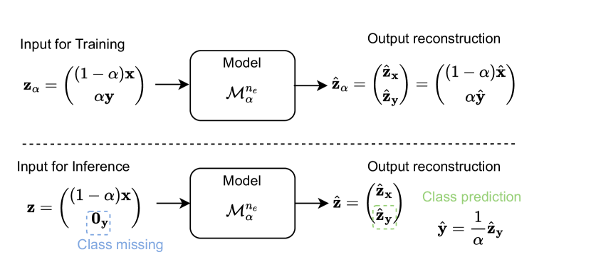
Fig. 3: Using model $\mathcal{M}^{n_{e}}_{\alpha}$: At training stage, hyper-parameters $\alpha$ and $n_{e}$ are chosen, principal components $\mathrm{U}_{\alpha}^{n_{e}}$ are computed as parameters for model $\mathcal{M}^{n_{e}}_{\alpha}$. Note that the reconstruction error $\mathbb{E}_{\mathcal{T}_{\alpha}}[\|\mathbf{z}_{\alpha}-\hat{\mathbf{z}_{\alpha}}\|]$ is minimized when using $\mathrm{U}_{\alpha}^{n_{e}}$. At test time, the input used is proportional to $\mathbf{z}_{0}$ and a class prediction appears as part of the output reconstruction.

From the output $\hat{\mathbf{z}}$, the subvector $\hat{\mathbf{y}}$ is analysed such that the class $j\in\{1,\cdots,n_{c}\}$ is identified by locating the highest valued coordinate of vector $\hat{\mathbf{y}}$:

$$\hat{j}=\arg\max_{j=1,\cdots,n_{c}}\left\{\hat{\mathbf{y}}^{T}=[\hat{y}_{1},\cdots,\hat{y}_{j},\cdots,\hat{y}_{n_{c}}]\right\}$$ (6)

Estimates $\hat{\mathbf{y}}$ can also be visualised in the $\mathbf{y}$-space (cf. Fig. 4).

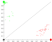
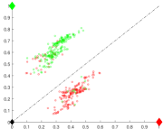
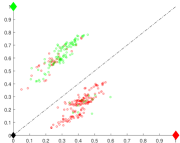
$\mathcal{I}^{\mathbf{x}}_{\mathbf{y}}$: acc=1	$\mathcal{I}^{\mathbf{x}}_{0}$: acc=0.8725	$\mathcal{I}^{\mathbf{x^{\prime}}}_{0}$: acc=0.8310

Fig. 4: Visualisation in the $\mathbf{y}$-space. Dataset australian: visualisation of the outputs $\hat{\mathbf{y}}$ (dots colour coded with the ground truth class label) in the class $\mathbf{y}$-space of dimension $n_{c}=2$ computed with model $\mathcal{M}^{n_{e}=4}_{\alpha=0.5}$. The black diamond shows the class input to our model for sets $\mathcal{I}^{\mathbf{x}}_{0}$ and $\mathcal{I}^{\mathbf{x^{\prime}}}_{0}$; the red and green diamonds are the ideal class vectors used as part of the input in set $\mathcal{I}^{\mathbf{x}}_{\mathbf{y}}$ (cf. Sec. 3).

3 Experimental results

We rescale feature vectors $\mathbf{x}$ so that the $\mathbf{x}$-space is an hypercube of volume 1. For MNIST dataset, all pixel values are scaled between 0 and 1 by dividing by 255. For the wine and australian datasets, all feature dimensions are re-scaled to 1 by dividing by their corresponding maximum found in the dataset. For the australian dataset, we have used 200 instances per class for creating a balanced training set $\mathcal{B}$ ($N=2\times 200=400$) and the remaining $N^{\prime}=290$ instances are used for the set $\mathcal{B}^{\prime}$ (a random allocation of instances is performed between $\mathcal{B}$ and $\mathcal{B}^{\prime}$). Likewise for the wine dataset, 40 instances per class are used for creating a balanced training set $\mathcal{B}$ ($N=3\times 40=120$) and the rest $N^{\prime}=58$ is used for the test set $\mathcal{B}^{\prime}$ (random allocation is performed at every run). For the MNIST dataset, 1000 instances per class is used for training ($N=10\times 1000=10000$) and a balanced test set is likewise defined with $N^{\prime}=10\times 1000=10000$ exemplars.

From the training set $\mathcal{B}=\{(\mathbf{x}^{(i)},\mathbf{y}^{(i)})\}_{i=1,\cdots,N}$, the set $\mathcal{T}_{\alpha}=\{\mathbf{z}_{\alpha}^{(i)}\}$ is used to compute the matrix of eigenvectors $\mathrm{U}_{\alpha}$. It is also used as a set of inputs noted $\mathcal{I}^{\mathbf{x}}_{\mathbf{y}}\equiv\mathcal{T}_{\alpha}$ for testing our model $\mathcal{M}^{n_{e}}_{\alpha}$: both feature vectors and class vectors are available as seen during training of the model $\mathcal{M}^{n_{e}}_{\alpha}$ therefore we expect accuracy reported for $\mathcal{I}^{\mathbf{x}}_{\mathbf{y}}$ to be high if not perfect when the number $n_{e}$ of eigenvectors is large enough to prevent any loss of information. In practice the class vector is not known and only the feature vector is available to be used as input of the our model $\mathcal{M}^{n_{e}}_{\alpha}$ (cf. Fig. 3). We propose to use the input $\mathbf{z}_{0}$ (multiply by $(1-\alpha)$, cf. Eq. 1) that initialises all components in the class vector to 0s. From the training set $\mathcal{B}=\{(\mathbf{x}^{(i)},\mathbf{y}^{(i)})\}_{i=1,\cdots,N}$, we create a test set of inputs noted $\mathcal{I}_{0}^{\mathbf{x}}=\{(1-\alpha)\mathbf{z}_{0}^{(i)}\}$ that have the same feature vectors as seen during training by the model but without its class information. From $\mathcal{B}^{\prime}$ unseen for computing the matrix $\mathrm{U}_{\alpha}$, we create likewise a set of inputs noted $\mathcal{I}_{\mathbf{0}}^{\mathbf{x^{\prime}}}$ to test our model for classification. For each set of inputs $\mathcal{I}^{\mathbf{x}}_{\mathbf{y}}$, $\mathcal{I}^{\mathbf{x}}_{\mathbf{0}}$ and $\mathcal{I}^{\mathbf{x^{\prime}}}_{\mathbf{0}}$, our model is used to estimate the class label (cf. Eq. 6) and we report the accuracy rate.

Figure 5 shows classification accuracies colour coded as heat maps computed for sets $\mathcal{I}^{\mathbf{x}}_{\mathbf{y}}$, $\mathcal{I}^{\mathbf{x}}_{\mathbf{0}}$ and $\mathcal{I}^{\mathbf{x^{\prime}}}_{\mathbf{0}}$, for a range of values $0\leq\alpha\leq 1$ and $n_{e}\in\{1,2,\cdots,d_{\mathbf{z}}\}$. In practice, the hyper-parameters $n_{e}$ and $\alpha$ can be chosen with grid search on these heat-maps computed with $\mathcal{I}^{\mathbf{x}}_{\mathbf{0}}$ (acting as validation set) in order to get the best accuracy possible for the minimum number $n_{e}$ of principal components that affect the computational cost of our model. As expected, results on set $\mathcal{I}^{\mathbf{x}}_{\mathbf{y}}$ often reach perfect accuracy (Acc=1). The classification accuracy for sets $\mathcal{I}^{\mathbf{x}}_{\mathbf{0}}$ and $\mathcal{I}^{\mathbf{x}^{\prime}}_{\mathbf{0}}$ has a similar behaviour showing that our approach generalised well to unseen features.

For MNIST dataset, heat-maps look smooth on the hyper-parameter space and we see that increasing $\alpha$ allows to concentrate classification efficiency on the first $16$ eigenvectors for $\mathcal{I}^{\mathbf{x}}_{\mathbf{0}}$ and $\mathcal{I}^{\mathbf{x}^{\prime}}_{\mathbf{0}}$ (cf. Fig. 5). The classification accuracy for $\mathcal{I}^{\mathbf{x}}_{\mathbf{0}}$ and $\mathcal{I}^{\mathbf{x}^{\prime}}_{\mathbf{0}}$ decreases when too many eigenvectors are used: our model approximates (and converge to) the identity function (when $n_{e}=d_{\mathbf{z}}$, cf. Eq. (5) ) and therefore the model output corresponds to its input which does not provide any class prediction for $\mathcal{I}^{\mathbf{x}}_{\mathbf{0}}$ and $\mathcal{I}^{\mathbf{x}^{\prime}}_{\mathbf{0}}$. However, when compressing information in the encoder (i.e. choosing $n_{e}<<d_{\mathbf{z}}$), a class prediction appears as part of the output. For fair benchmark comparison, our models $\mathcal{M}_{0.9}^{16}$ and $\mathcal{M}_{0.02}^{618}$ are retrained on the full training set (no data augmentation), and classification accuracy is computed for the full provided test set (cf. Tab 1).

Model	Accuracy	# Trainable para.
Ours $\mathcal{M}_{0.9}^{16}$	0.8093	12704
Ours $\mathcal{M}_{0.02}^{618}$	0.8541	490692
Efficient-CapsNet [8]	0.99	161000
LeNet [5]	0.99	60000

Table 1: Benchmark on MNIST. Accuracy result reported for our models $\mathcal{M}_{0.9}^{16}$ and $\mathcal{M}_{0.02}^{618}$ (trained here on the $N=60,000$ images) is computed using the full test set ($N^{\prime}=10,000$ test images). Its number of trainable parameters corresponds to the number of elements in matrix $\mathrm{U}_{\alpha}^{n_{e}}$ (i.e. $n_{e}\times d_{\mathbf{z}}$). While not competing for acuracy with deep learning models, our results with our models took less than 2 seconds for each $\mathcal{M}_{0.9}^{16}$ and $\mathcal{M}_{0.02}^{618}$ to compute -both training and testing - in this experiment highlighting how frugal our model is.

$\mathcal{I}^{\mathbf{x}}_{\mathbf{y}}$	$\mathcal{I}^{\mathbf{x}}_{0}$	$\mathcal{I}^{\mathbf{x^{\prime}}}_{0}$
Dataset australian: $n_{c}=2$, $N=n_{c}\times 200$, $N^{\prime}=290$, $d_{\mathbf{x}}=14$, $d_{\mathbf{z}}=16$. Accuracy results reported in [4] using the entire 14 dimensional feature space, range in between 0.65 to 0.85. Our model $\mathcal{M}_{0.2}^{4}$ has average classification accuracy rates ($\pm$standard deviations) of $(0.81\pm 0.03;0.77\pm 0.02;0.76\pm 0.02)$ for sets $(\mathcal{I}^{\mathbf{x}}_{\mathbf{y}};\mathcal{I}^{\mathbf{x}}_{0};\mathcal{I}^{\mathbf{x^{\prime}}}_{0})$ computed over 10 runs. With an additional principal component, our models $\mathcal{M}_{0.2}^{5}$ and $\mathcal{M}_{0.4}^{5}$ have classification accuracy rates $(0.86\pm 0.01;0.86\pm 0.01;0.84\pm 0.02)$ and $(0.98\pm 0.007;0.86\pm 0.01;0.84\pm 0.02)$ respectively.
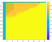
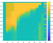
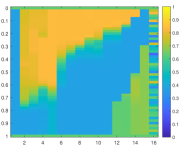
Dataset wine: $n_{c}=3$, $N=n_{c}\times 40$, $N^{\prime}=58$, $d_{\mathbf{x}}=13$, $d_{\mathbf{z}}=16$. Accuracy results reported in [16, 4, 7] using the entire 13 dimensional feature space, range in between 0.70 to 0.98. Our model $\mathcal{M}_{0.2}^{4}$ has average classification accuracy rates ($\pm$standard deviations) of $(0.99\pm 0.005;0.94\pm 0.02;0.88\pm 0.03)$ for sets $(\mathcal{I}^{\mathbf{x}}_{\mathbf{y}};\mathcal{I}^{\mathbf{x}}_{0};\mathcal{I}^{\mathbf{x^{\prime}}}_{0})$ computed over 10 runs. With an additional principal component, our models $\mathcal{M}_{0.2}^{5}$ and $\mathcal{M}_{0.4}^{5}$ have classification accuracy rates $(0.99\pm 0.003);0.96\pm 0.01;0.92\pm 0.02)$ and $(1.00\pm 0;0.95\pm 0.02;0.91\pm 0.02)$ respectively.
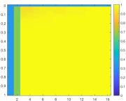
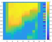
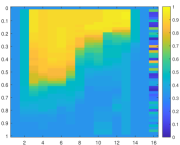
Dataset MNIST: $n_{c}=10$, $N=n_{c}\times 1000$, $N^{\prime}=n_{c}\times 1000$, $d_{\mathbf{x}}=784$, $d_{\mathbf{z}}=794$. [6] reports accuracy ranging between 0.93 to 0.99 in reduced space of 164 dimensions, [4] reports accuracy ranging between 0.82 to 0.88 using the entire 784 dimensional feature space dimensions. Our model $\mathcal{M}_{0.2}^{164}$ has accuracy rates $(0.8661;0.8598;0.8247)$ for sets $(\mathcal{I}^{\mathbf{x}}_{\mathbf{y}};\mathcal{I}^{\mathbf{x}}_{0};\mathcal{I}^{\mathbf{x^{\prime}}}_{0})$. With only 16 principal components, our model $\mathcal{M}_{0.9}^{16}$ has also a good performance $(1.00;0.8089;0.7883)$ for a much lower computational cost.

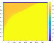
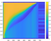
Fig. 5: Classification accuracy rate (colour coded) over the hyper-parameter space $n_{e}=[1:1:d_{\mathbf{z}}]$ (abscissa) and $\alpha=[0:0.02:1]$ (y-axis), with comparison to KNN classification results using metric learning [16, 4, 7].

4 Conclusion

We have introduced a new linear, PCA inspired, classifier that has encouraging accuracy, can learn from small training datasets as well as larger ones. It has very low computational complexity compared to deep learning models. Future work will investigate combining multiple models learning from smaller image patches (as done in CNNs) to improve accuracy on image dataset (ensemble learning), and what alternative strategy to grid search could be used to select hyper-parameters.

References

- [1] Rosanne Liu, Joel Lehman, Piero Molino, Felipe Petroski Such, Eric Frank, Alex Sergeev, and Jason Yosinski, “An intriguing failing of convolutional neural networks and the coordconv solution,” in Advances in Neural Information Processing Systems, S. Bengio, H. Wallach, H. Larochelle, K. Grauman, N. Cesa-Bianchi, and R. Garnett, Eds. 2018, vol. 31, Curran Associates, Inc.
- [2] Ben Mildenhall, Pratul P. Srinivasan, Matthew Tancik, Jonathan T. Barron, Ravi Ramamoorthi, and Ren Ng, “Nerf: Representing scenes as neural radiance fields for view synthesis,” Commun. ACM, vol. 65, no. 1, pp. 99–106, dec 2021.
- [3] Dheeru Dua and Casey Graff, “UCI machine learning repository,” 2017, http://archive.ics.uci.edu/ml.
- [4] Pourya Habib Zadeh, Reshad Hosseini, and Suvrit Sra, “Geometric mean metric learning,” in Proceedings of the 33rd International Conference on International Conference on Machine Learning - Volume 48. 2016, ICML’16, p. 2464–2471, JMLR.org.
- [5] Y. Lecun, L. Bottou, Y. Bengio, and P. Haffner, “Gradient-based learning applied to document recognition,” Proceedings of the IEEE, vol. 86, no. 11, pp. 2278–2324, 1998.
- [6] Kilian Q. Weinberger and Lawrence K. Saul, “Distance metric learning for large margin nearest neighbor classification,” J. Mach. Learn. Res., vol. 10, pp. 207–244, jun 2009.
- [7] A. Collas, A. Breloy, G. Ginolhac, C. Ren, and J.-P. Ovarlez, “Robust geometric metric learning,” in 30th European Signal Processing Conference (EUSIPCO), Belgrade, Serbia, 2022.
- [8] V. Mazzia, F. Salvetti, and M. Chiaberge, “Efficient-capsnet: capsule network with self-attention routing,” Scientific Reports, vol. 11, no. 14634, 2021.
- [9] F. van der Heijden, R. P. W. Duin, D. de Ridder, and D. M.J. Tax, Classification, Parameter Estimation and State estimation; An Engineering Approach using Matlab, Wiley, 2004.
- [10] B. Moghaddam and A. Pentland, “Probabilistic visual learning for object representation,” IEEE Transactions on Pattern Analysis and Machine Intelligence, vol. 19, no. 7, pp. 696–710, 1997.
- [11] R. Dahyot, P. Charbonnier, and F. Heitz, “A bayesian approach to object detection using probabilistic appearance-based models,” Pattern Analysis and Applications, vol. 7, no. 3, pp. 317–332, Dec 2004.
- [12] C. Arellano and R. Dahyot, “Robust bayesian fitting of 3d morphable model,” in Proceedings of the 10th European Conference on Visual Media Production, New York, NY, USA, 2013, CVMP ’13, pp. 9:1–9:10, ACM, http://doi.acm.org/10.1145/2534008.2534013.
- [13] Michael E. Tipping and Christopher M. Bishop, “Probabilistic principal component analysis,” Journal of the Royal Statistical Society. Series B (Statistical Methodology), vol. 61, no. 3, pp. 611–622, 1999.
- [14] J. Chopin, J.-B. Fasquel, H. Mouchere, R. Dahyot, and I. Bloch, “Improving semantic segmentation with graph-based structural knowledge,” in ICPRAI International Conference on Pattern Recognition and Artificial Intelligence, 2022.
- [15] Ian Gemp, Brian McWilliams, Claire Vernade, and Thore Graepel, “EigenGame: PCA as a nash equilibrium,” in International Conference on Learning Representations, 2021.
- [16] Laurens van der Maaten and Geoffrey Hinton, “Visualizing data using t-sne,” Journal of Machine Learning Research, vol. 9, no. 86, pp. 2579–2605, 2008.