Self-testing of different entanglement resources via fixed measurement settings

Abstract

Self-testing, which refers to device independent characterization of the state and the measurement, enables the security of quantum information processing task certified independently of the operation performed inside the devices. Quantum states lie in the core of self-testing as key resources. However, for the different entangled states, usually different measurement settings should be taken in self-testing recipes. This may lead to the redundancy of measurement resources. In this work, we use fixed two-binary measurements and answer the question that what states can be self-tested with the same settings. By investigating the structure of generalized tilted-CHSH Bell operators with sum of squares decomposition method, we show that a family of two-qubit entangled states can be self-tested by the same measurement settings. The robustness analysis indicates that our scheme is feasible for practical experiment instrument. Moreover, our results can be applied to various quantum information processing tasks.

I Introduction

Bell nonlocality CHSH1969 ; Nonlocality2014 is central to the understanding of quantum physics. With the advent of quantum information, Bell nonlocality has been studied as a resource and applied to various quantum information processing tasks, such as quantum key distribution DIQKD2007 ; DIQKD2014 , randomness expansion DIQRNG2010 ; DIQRNG2018 and entanglement witness DIEW2013 ; DIEW2018 .

Moreover, if we assume quantum mechanics to be the underlying theory, it is shown that certain extremal quantum correlations uniquely identify the state and measurements under consideration, a phenomenon known as self-testing Mayers2004 ; 2012Scarani . It is a concept of device independence whose conclusion verdict relies only on the observed statistics of measurement outcomes under the sole assumptions of no-signaling and the validity of quantum theory Supic2020 . In 1990s, Popescu and Rohrlich et al. pointed out that the maximal violation of the Clauser–Horne–Shimony–Holt (CHSH) Bell inequality identifies uniquely the maximally entangled state of two qubit Tsirelson ; MI2011Gisin . In the last decades, self-testing has received substantial attention. The scenarios for bipartite and multipartite entangled states were presented in Refs. 2017Coladangelo ; 2015Bamps ; 2017Coladangelo ; 2016Wang ; Wu1 ; 2014Wu ; McKague2 ; 2018Li ; 2020Li . The robustness analysis to small deviations from the ideal case for self-testing these quantum states and measurements were presented in Refs. 2016Kaniewski ; 2019LWH ; Bancal ; 2019Coopmans , which made self-testing more practical. Beyond these works focusing on the single copy states, the parallel self-testing of tensor product states have recently been studied. The first parallel self-testing protocol was proposed for 2 EPR pairs in 2016Wu . The result was subsequently generalised for arbitrary $n$, via parallel repetition of the CHSH game in Coladangelo and via parallel repetition of the magic square game in Coudron . Self-testing of $n$ EPR pairs via parallel repetition of the Mayers-Yao self-test is given in 2016McKague .

In the most previous scenario, one measurement setting is always competent to self-test one target state up to local unitaries. For example, the tilted-CHSH inequality can self-test two-qubit pure states $\ket{\psi(\theta)}=\cos\theta\ket{00}+\sin\theta\ket{11}$ with corresponding measurements settings $\{\sigma_{z},\sigma_{x}\}\otimes\{\cos\mu\sigma_{z}+\sin\mu\sigma_{x},\cos\mu\sigma_{z}-\sin\mu\sigma_{x}\}$, meanwhile $\mu$ is uniquely determined by $\theta$. However, the tasks of quantum information processing may involve multiple states with different entanglement degree 2020Wagner . The whole self-testing of quantum states results in an increased consumption of the measurement resource, thus strike the feasibility of practical realization. Therefore, self-testing protocol with high practical performance is meaningful and necessary. In this work, we focus on this goal and provide a device independent scheme that certify a series of quantum states with reduced measurement resource. Our results show that the generalized tilted-CHSH operators allow the optimal measurements for one party could rotate on Pauli $x-z$ plane. Multiple different target states can be self-tested via a common measurement settings by choosing proper generalized tilted-CHSH operator. Hence, by utilizing a set of Bell inequalities, we can self-test two-qubit states with different entanglement degree only based on two binary measurements per party. Thus our scheme simplifies the measurement instruments and leads to less consumption of measurement resources. Besides, our scheme demonstrates satisfactory robustness in tolerance of noise. Further, our scheme can serve for various quantum information processing tasks with low measurement resources cost, meanwhile provides secure certification of the device used in the task. The paper is structured as follows: In Sec. II.1, we give a brief description about the underlying model and key definitions of our work. In Sec. II.2, we propose a scheme that self-tests different two-qubit entangled states via the same measurements using generalized tilted-CHSH inequality. During this study, we develop a family of self-testing criteria beyond the standard tilted-CHSH inequality and prove these criteria using the technique of sum-of-squares (SOS) decomposition. In Sec. III, the robustness analysis is illustrated through an example by the swap method and semidefinite programming (SDP). In Sec. IV, the applications of our results on quantum information processing tasks of device independent quantum key distribution, private query and randomness generation are presented. In Sec.V, we summarize the results and discuss the future research.

II Self-testing different entangled states via two binary measurements

II.1 Self-testings

Consider the simplest scenario of two noncommunicating parties, Alice and Bob. Each has access to a black box with inputs denoted respectively by $x,y\in\{0,1\}$ and outputs $a,b\in\{+1,-1\}$. One could model these boxes with an underlying state $\ket{\psi}_{AB}$ and measurement projectors $\left\{M_{x}^{a}\right\}_{x,a}$ and $\left\{M_{y}^{b}\right\}_{y,b}$, which commute for different parties. The state can be taken pure and the measurements can be taken projective without loss of generality, because the dimension of the Hilbert space is not fixed and the possible purification and auxiliary systems can be given to any of the parties. After sufficiently many repetitions of the experiment one can estimate the joint conditional statistics, as known as the behavior, $p(a,b|x,y)=\bra{\psi}M_{x}^{a}M_{y}^{b}\ket{\psi}$. Self-testing refers to a device-independent certification way where the nontrivial information on the state and the measurements is uniquely certified by the observed behavior $p(ab|xy)$, without assumptions on the underlying degrees of freedom. Usually, self-testing can be defined formally in the following way.

Definition 0.1.

We say that the correlations $p(a,b|x,y)$ allow for self-testing if for every quantum behavior $(\ket{\psi}$, $\{M_{x}^{a},M_{y}^{b}\})$ compatible with $p(a,b|x,y)$ there exists a local isometry $\Phi=\Phi_{A}\otimes\Phi_{B}$ such that

$$\Phi\ket{\psi}_{AB}\ket{00}_{A^{\prime}B^{\prime}} =\ket{junk}_{AB}\otimes\ket{\overline{\psi}}_{A^{\prime}B^{\prime}}$$ (1)

$$\Phi(M^{a}_{x}\ket{\psi}_{AB}\ket{00}_{A^{\prime}B^{\prime}}) =\ket{junk}_{AB}\otimes\overline{M^{a}_{x}}\ket{\overline{\psi}}_{A^{\prime}B^{\prime}},$$

where $|00\rangle_{A^{\prime}B^{\prime}}$ is the trusted auxiliary qubits attached by Alice and Bob locally into their systems, $(\ket{\overline{\psi}},\{\overline{M_{x}^{a}},\overline{M_{y}^{b}}\})$ are the target system 2012Scarani .

That is the correlations $p(a,b|x,y)$ predicted by quantum theory could determine uniquely the state and the measurements, up to a local isometry.

II.2 Self-testing of entangled two-qubit states with generalized tilted-CHSH inequality

In this section, we show that different pure entangled two-qubit states can be self-tested via fixed measurement setting with generalized tilted-CHSH inequality. The candidate target states we considered are $\{\ket{\overline{\psi}_{i}}\}$, with

$$\ket{\overline{\psi}_{i}} =\cos\theta_{i}\ket{00}+\sin\theta_{i}\ket{11}$$ (2)

where $\theta_{i}\in(0,\frac{\pi}{4}]$. It is already proved that pure entangled two-qubit state can be self-tested using standard tilted-CHSH inequality 2015Bamps ; 2019Coopmans . In the standard scheme, one measurement setting is required for self-testing one target state, which results in an increased consumption of the measurement resource. Utilizing the property of generalized generalized tilted-CHSH inequality, we show that all these entangled states can be self-tested with the given fixed measurements, thus simplifies the measurement instruments. We have the following theorem.

Theorem 1.

The family of entangled two-qubit states in Eq. (2) can be self-tested by the same quantum measurement settings in Eq. (II.2) with fixed angle $\mu$. The fact of the self-testing result comes from the maximum quantum violation of generalized tilted-CHSH inequalities in Eq. (4).

The measurements in our scheme are chosen as,

$$A_{0} =\sigma_{z},\;\;B_{0}=\cos\mu\sigma_{z}+\sin\mu\sigma_{x}$$

$$A_{1} =\sigma_{x},\;\;B_{1}=\cos\mu\sigma_{z}-\sin\mu\sigma_{x}$$ (3)

with the fixed angle $\mu\in(0,\frac{\pi}{4}]$.

The key idea of our self-testing scheme is that for a given $\mu$ in the unit measurement settings, a family of Bell inequalities can be maximally violated by different entangled pairs respectively at the same time. Once the form of the target source is confirmed, the Bell inequality which achieve their self-testing are determined based on the observed statistics, $p(a,b|x,y)$. More precisely, the Bell inequalities have the form conditional on the input $i\in\{0,1,2,..,n\}$ as

$$\mathcal{B}_{[\alpha_{i},\beta_{i}]}= \beta_{i}A_{0}+\alpha_{i}(A_{0}B_{0}+A_{0}B_{1})+A_{1}B_{0}-A_{1}B_{1},$$ (4)

named generalized tilted CHSH inequality Acin2012 , where $\alpha_{i}\geq 1$. The maximal classical and quantum bounds are $C_{[\alpha_{i},\beta_{i}]}=2\alpha_{i}+\beta_{i}$ and $\eta_{[\alpha_{i},\beta_{i}]}=\sqrt{(4+\beta_{i}^{2})(1+\alpha_{i}^{2})}$, respectively. It is already proved both theoretically and numerically that pure entangled two-qubit state can be self-tested using standard tilted-CHSH inequality with $\alpha=1$ in Eq. (4) 2015Bamps ; 2019Coopmans . However, whether generalized tilted-CHSH inequality can be used in self-testing is still unknown.

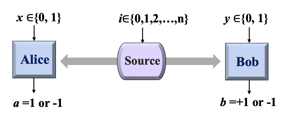
Figure 1: Self-testing recipe. The fixed untrusted measurements setting are able to test different input states. For a given a target state $\ket{\overline{\psi}_{i}}$, two observers randomly chose their measurement $x$ for Alice, $y$ for Bob, and collect outcomes $a$ and $b$ to construct the observation of $\mathcal{B}_{[\alpha_{i},\beta_{i}]}$.

We claim that the maximal quantum violation in Eq. (4) uniquely certify the corresponding entangled pairs in Eq. (2) and measurements in Eq. (II.2) with $\sin 2\theta_{i}=\sqrt{\frac{4-\alpha_{i}^{2}\beta_{i}^{2}}{4+\beta_{i}^{2}}}$ and $\tan\mu=\frac{\sin 2\theta_{i}}{\alpha_{i}}$. Thus the family of pure entangled two-qubit states are self-tested with the given $\alpha$, $\beta$ and the fixed two measurement settings $\mu$ using generalized tilted-CHSH inequality. The self-testing recipe of our scheme is shown in Fig. 1. In the following, we give the detailed proof of Theorem 1.

Proof. The proof of Theorem 1 is divided into two steps. First, we give two types of SOS decompositions for generalized tilted-CHSH operator $\mathcal{B}_{[\alpha,\beta]}$ (see Appendix for details). Moreover, these SOS decompositions establish algebraic relations that are necessarily satisfied by any quantum state and observables yielding maximal violation of the generalized tilted-CHSH inequality. Then these algebraic relations are used in the isometry map to provide the self-testing of any partially entangled two-qubit state.

a. SOS decompositions for generalized tilted-CHSH inequalities. The generalized tilted-CHSH inequalities $\mathcal{B}_{[\alpha,\beta]}$ have the maximum quantum violation value $\eta_{[\alpha,\beta]}$. This implies that the operator $\widehat{\mathcal{B}}=\eta_{[\alpha,\beta]}\mathbb{I}-\mathcal{B}_{[\alpha,\beta]}$ is positive semidefinite for all possible quantum states and measurement operators $A_{x}$ and $B_{y}$. This can be proven by providing a set of operators $\{P_{i}\}$ which are polynomial functions of $A_{x}$ and $B_{y}$ such that $\widehat{\mathcal{B}}_{[\alpha,\beta]}=\sum_{i}P^{\dagger}_{i}P_{i}$, holds for any set of measurement operators satisfying the algebraic properties $A^{2}_{x}=\mathbb{I}$, $B^{2}_{y}=\mathbb{I}$ and $[A_{x},B_{y}]=0$.

For convenience, we define three classes CHSH operators:

$$S_{0} =A_{0}(B_{0}-B_{1})+\frac{1}{\alpha}A_{1}(B_{0}+B_{1}),$$

$$S_{1} =\frac{1}{\alpha}A_{0}(B_{0}+B_{1})-A_{1}(B_{0}-B_{1}),$$ (5)

$$S_{2} =A_{0}(B_{0}-B_{1})-\alpha A_{1}(B_{0}+B_{1}).$$

Then we can give two types of SOS decompositions for generalized tilted-CHSH operator in Eq. (4). The first decomposition is given as

$$\widehat{\mathcal{B}}_{[\alpha,\beta]}= \frac{1}{\Delta+2\eta_{[\alpha,\beta]}}\{(\widehat{\mathcal{B}}_{[\alpha,\beta]})^{2}+\alpha^{2}(\beta A_{1}-S_{0})^{2}$$

$$+(\alpha^{2}-1)[({\color[rgb]{0,0,0}-}\beta A_{0}+\frac{\eta_{[\alpha,\beta]}}{\alpha^{2}+1}-A_{1}(B_{0}-B_{1}))^{2}$$

$$+(-\frac{\eta_{[\alpha,\beta]}\alpha}{\alpha^{2}+1}A_{0}+B_{0}+B_{1})^{2}]\}.$$ (6)

And the second one is

$$\widehat{\mathcal{B}}_{[\alpha,\beta]}= \frac{\alpha^{2}}{\Delta+2\eta_{[\alpha,\beta]}}\big{\{}\frac{\alpha^{2}-1}{\alpha^{2}}[(-\frac{\eta_{[\alpha,\beta]}\alpha}{\alpha^{2}+1}A_{0}+B_{0}+B_{1})^{2}$$

$$+({\color[rgb]{0,0,0}-}\beta A_{0}+\frac{\eta_{[\alpha,\beta]}}{\alpha^{2}+1}-A_{1}(B_{0}-B_{1}))^{2}]$$

$$+\big{(}2A_{0}-\frac{\eta_{[\alpha,\beta]}}{2\alpha}(B_{0}+B_{1})+\frac{\beta}{2}S_{1})^{2}$$

$$+\frac{1}{{\color[rgb]{0,0,0}\alpha^{2}}}(2A_{1}-\frac{\eta_{[\alpha,\beta]}}{2}(B_{0}-B_{1})+\frac{\beta}{2}S_{2})^{2}\big{\}}$$ (7)

where $\Delta=2(\alpha^{2}-1)\sqrt{\frac{\beta^{2}+4}{\alpha^{2}+1}}$.

For the special case $\alpha=1$ of standard tilted-CHSH inequality, our result gives the following decomposition:

$$\widehat{\mathcal{B}}_{[1,\beta]}=\frac{1}{2\eta_{[1,\beta]}}[(\widehat{\mathcal{B}}_{[1,\beta]})^{2}+(\beta A_{1}-S_{0})^{2}],$$ (8)

and

$$\widehat{\mathcal{B}}_{[1,\beta]}= \frac{1}{2\eta_{[1,\beta]}}[(2A_{0}-\eta_{[1,\beta]}\frac{B_{0}+B_{1}}{2}+\frac{\beta}{2}S_{1})^{2}$$

$$+(2A_{1}-\eta_{[1,\beta]}\frac{B_{0}-B_{1}}{2}+\frac{\beta}{2}S_{2})^{2}],$$ (9)

which reproduce the results in Ref. 2015Bamps . Thus we develop a family of SOS decompositions for generalized tilted-CHSH inequalities, which is beyond the standard form.

If one observes the maximal quantum violation of the generalized tilted-CHSH inequality in Eq. (4) by any state $\ket{\psi}$ and measurements $A_{x}$, $B_{y}$ for $x,y\in\{0,1\}$, then each square of polynomial functions in two SOS decompositions acting on $\ket{\psi}$ is equal to zero, i.e., $P_{i}\ket{\psi}=0$. Then we can obtain the anti-commutation relations for the measurements operators acting on the underlying state from the two SOS decompositions (II.2)–(II.2) as following (the details refer to Appendix)

$$(Z_{A}-Z_{B})\ket{\psi} =0,$$ (10a)

$$(\sin\theta X_{A}(\mathbb{I}+Z_{B})-\cos\theta X_{B}(\mathbb{I}-Z_{A}))\ket{\psi} =0.$$ (10b)

Next we will show that these algebraic relations lead to self-testing statement for any partially entangled two-qubit state.

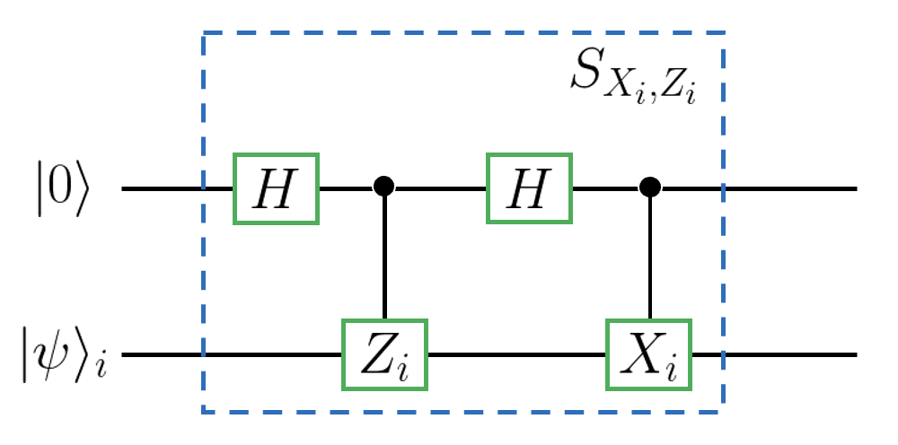
Figure 2: The local unit $S_{i}$ of the swap gate $S=S_{A}\otimes S_{B}$ for $i\in\{A,B\}$. Each unit acts on the corresponding particle of the $\ket{\psi}$ and one ancillary qubit prepared in the state $\ket{0}$. $H$ is the standard Hadamard gate, $Z_{i}$ and $X_{i}$ are controlled by the auxiliary qubits.

b. Self-testing of partially entangled states. Basing on the Definition 0.1 of self-testing, one needs to construct the isometry map such that the underlying system can extract out the information of target state. The isometry is a virtual protocol, all that must be done in laboratory is to query the boxes and derive $p(a,b|x,y)$. The useful way is so-called swap method and the isometry is shown in Fig. 2. The idea of swap method is from the ideal case. If the state $\ket{\psi}$ is indeed two-qubit and the operators are $Z=\sigma_{z}$, $X=\sigma_{x}$, the swap operations could extract the state $\ket{\psi}$ into ancilla system. However, in the device-independent framework, it can not assume the dimension of the inner state or any form of the operators. Hence $Z$ and $X$ are constructed basing on real performed measurements $A_{x}$ and $B_{y}$ such that one can swap out the desired states and measurements, as shown in Definition 0.1. Therefore, we define the unitary operators of Alice and Bob as

$$Z_{A}=A_{0},\;\;Z_{B} =\frac{B_{0}+B_{1}}{2\cos\mu},$$

$$X_{A}=A_{1},\;\;X_{B} =\frac{B_{0}-B_{1}}{2\sin\mu}.$$ (11)

After this isometry, the underlying systems and the trusted auxiliary qubits will be

$$\Phi(\ket{\psi})= \frac{1}{4}[(\mathbb{I}+Z_{A})(\mathbb{I}+Z_{B})\ket{\psi}\ket{00}$$

$$+X_{B}(\mathbb{I}+Z_{A})(\mathbb{I}-Z_{B})\ket{\psi}\ket{01}$$

$$+X_{A}(\mathbb{I}-Z_{A})(\mathbb{I}+Z_{B})\ket{\psi}\ket{10}$$

$$+X_{A}X_{B}(\mathbb{I}-Z_{A})(\mathbb{I}-Z_{B})]\ket{\psi}\ket{11}.$$ (12)

From relation (10a), the second and third terms of Eq. (II.2) cancel to be zero. Then relation (10b) eventually leads Eq. (II.2) to be

$$\Phi(\ket{\psi})= \frac{\mathbb{I}+Z_{A}}{2}\ket{\psi}\ket{00}+\frac{\mathbb{I}+Z_{A}}{2}\frac{\sin\theta}{\cos\theta}\ket{\psi}\ket{11}$$

$$= \ket{junk}\otimes\ket{\overline{\psi}},$$ (13)

where

$$\ket{junk}=\frac{\mathbb{I}+Z_{A}}{2\cos\theta}\ket{\psi}.$$ (14)

Thus the underlying state is equal to the optimal target form $\ket{\overline{\psi}}=\cos\theta\ket{00}+\sin\theta\ket{11}$ with $\sin 2\theta=\sqrt{\frac{4-\alpha^{2}\beta^{2}}{4+\beta^{2}}}$. This completes the self-testing statement.

The generalized tilted-CHSH operator $B_{[\alpha,\beta]}$ with two parameters such that the optimal measurements for one party could rotate on Pauli $x$-$z$ plane respect to the target one satisfying $\alpha\tan\mu={\sqrt{\frac{4-\alpha^{2}\beta^{2}}{4+\beta^{2}}}}$. It results in that in a self-testing scenario involving different target $\ket{\overline{\psi}_{i}}$ defined as Eq. (2), one can choose a common measurement settings (II.2) satisfying $\tan\mu=\frac{\sin 2\theta_{i}}{\alpha_{i}}$ to construct the Bell inequality $\eta_{[\alpha_{i},\beta_{i}]}$ for each target state. In turn, the maximal violations uniquely certify the family of states $\ket{\overline{\psi}_{i}}$. Thus, we complete the proof of Theorem 1.

To be specific, $\mathcal{B}_{[\alpha,\beta]}$ has two special forms when $\beta=0$ and $\alpha=1$, which corresponds to biased CHSH Lawson2010 and standard tilted-CHSH operators Bancal , respectively.

–Biased CHSH inequality. If $\beta=0$, the Bell inequality in Eq. (4) is simplified as a symmetrical biased CHSH operator

$$\mathcal{B}_{[\alpha,0]}=\alpha(A_{0}B_{0}+A_{0}B_{1})+A_{1}B_{0}-A_{1}B_{1}\leq 2\alpha,$$ (15)

where $\alpha=\frac{1}{\tan\mu}$, which belongs to the whole set of self-testing criteria for Bell state 2016Wang . Its maximal quantum violation $\eta_{[\alpha,0]}=\frac{4}{\sqrt{1+\tan\mu}}$ is able to self-test maximum entangled state $\ket{\overline{\psi}}=\frac{1}{\sqrt{2}}(\ket{00}+\ket{11})$ and measurements setting (II.2).

–Standard tilted-CHSH inequality. If $\alpha=1$, the Bell inequality in Eq. (4) turns to be the standard form

$$\mathcal{B}_{[1,\beta]}=\beta A_{0}+A_{0}B_{0}+A_{0}B_{1}+A_{1}B_{0}-A_{1}B_{1}\leq 2+\beta,$$ (16)

with $\beta=2\sqrt{2\cos^{2}\mu-1}$. The maximal quantum violation of this inequality is given by $\eta_{[1,\beta]}=\sqrt{8+2\beta^{2}}=4\cos\mu$, achievable with the measurement settings in Eq. (II.2) and satisfies $\sin 2\theta=\sqrt{\frac{4-\beta^{2}}{4+\beta^{2}}}$.

III robustness analysis

If the observed statistics deviate from the ideal ones, one can estimate how far the actual state and measurements are from the ideal ones, a property known as robustness. Here the robust self-testings of the different sources are analysed using numerical tool named Navascués-Pironio-Acín (NPA) hierarchy and SDP method NPA2008 ; Bancal . For convenience of calculations, we take $\mu=\arctan\frac{3}{4}$($\mu\approx 0.208\pi$) in measurements settings $\eqref{eq:M}$ as an example to self-test the following three sates

$$\ket{\overline{\psi}_{0}}= \frac{1}{\sqrt{2}}(\ket{00}+\ket{11}),$$

$$\ket{\overline{\psi}_{1}}= \cos\theta\ket{00}+\sin\theta\ket{11}\;\text{for }\theta=\frac{1}{2}\arcsin(\frac{3}{4}),$$

$$\ket{\overline{\psi}_{2}}= \frac{1}{2}(\ket{00}+\sqrt{3}\ket{11}),$$ (17)

which satisfy $\tan\mu=\frac{\sin 2\theta_{i}}{\alpha_{i}}$ with $\alpha_{0}=\frac{4}{3},\alpha_{1}=1$ and $\alpha_{2}=\frac{2}{\sqrt{3}}$. Choosing these three states not only associates with three special Bell operators (biased CHSH, standard tilted-CHSH and generalized tilted-CHSH operators), but also results in a convenience for the calculations in robustness analysis. To self-test these three target states, the parameter $\beta_{i}$ in Bell inequality (4) are set as $\beta_{0}=0$, $\beta_{1}=\frac{2\sqrt{7}}{5}$ and $\beta_{2}=\frac{2\sqrt{3}}{5}$ satisfying $\sin 2\theta_{i}=\sqrt{\frac{4-\alpha_{i}^{2}\beta_{i}^{2}}{4+\beta_{i}^{2}}}$, respectively. By substituting $[\alpha_{i},\beta_{i}]$ into $\mathcal{B}_{[\alpha_{i},\beta_{i}]}$ in Eq.(4) for $i=0,1,2$, it can be found the first two pairs respectively recover to biased inequality (15) and tilted-CHSH inequalities (16), while the third pair is complex. Particularly, by fixing $\tan\mu=\frac{3}{4}$, the parameter $\alpha$ can be express by $\beta$, i.e., $\alpha=\frac{8}{\sqrt{25\beta^{2}+36}}$, thus we can plot the bounds of Bell inequality $\mathcal{B}_{[\alpha_{i},\beta_{i}]}$ respect to $\beta$. As shown as in Fig. 3, with the increasing of $\beta$, the classical bound tends nearly but no more than the quantum. The maximal quantum bounds for the ideal self-testing of the three states (III) and measurement settings (II.2) are presented by red triangles in Fig. 3. The gap between classical and quantum bounds at $(\alpha_{0},\beta_{0})$ is much larger than the other points.

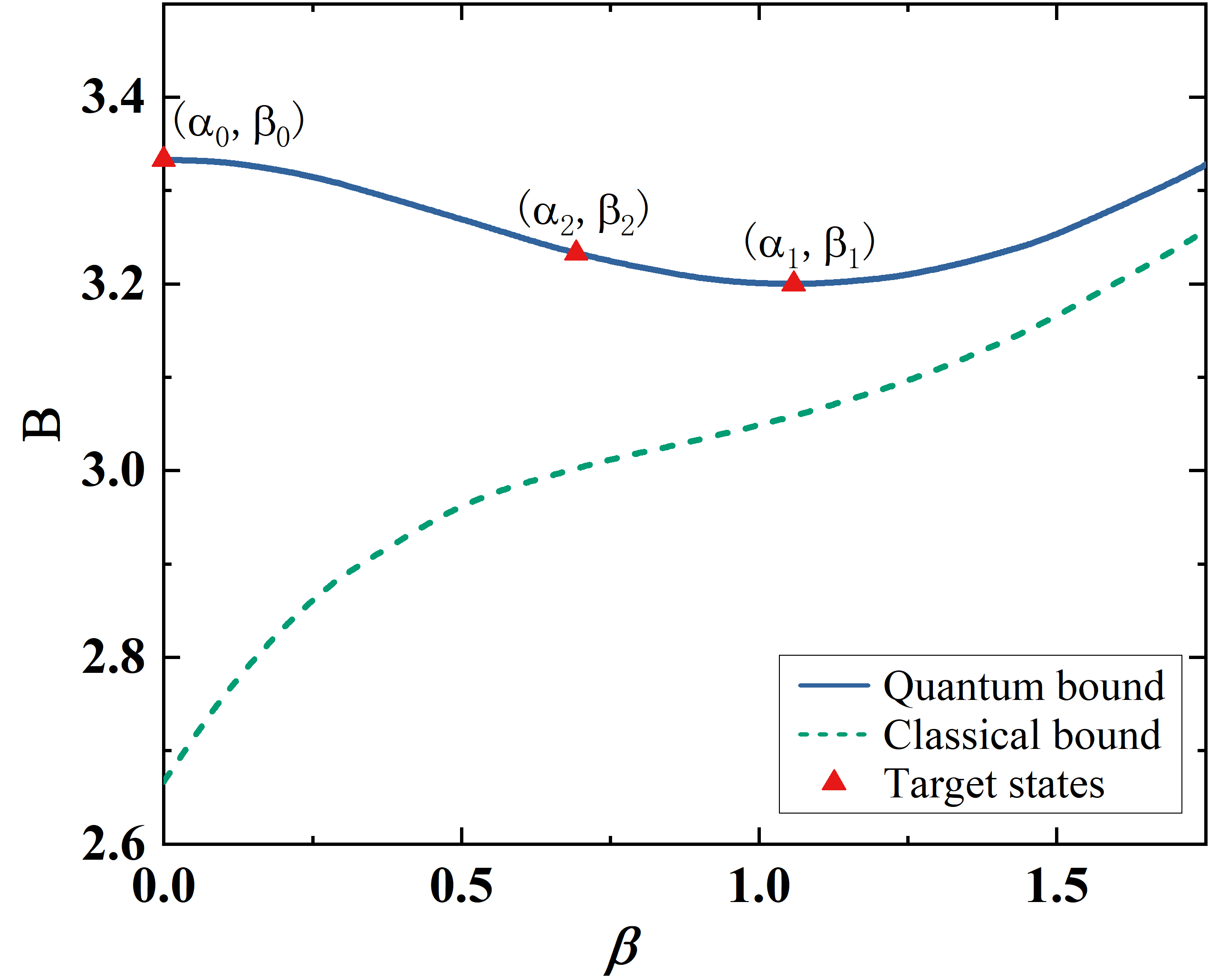
Figure 3: The maximal violations of Bell inequalities $\mathcal{B}_{[\alpha,\beta]}$ with respect to $\beta$ for $\tan\mu=3/4$. The blue solid and green dotted lines represent the maximal quantum and classical bounds, respectively. The red triangles on blue line are obtained with $[\alpha_{i},\beta_{i}]$ for i=0,1,2 which are ideal scenarios to self-test the three target states in Eq. (III).

After the isometry given in Fig. 2, the trusted auxiliary systems will be left in the state

$$\rho_{swap}=\sum_{ijst}C_{ijst}\ket{j}\bra{i}\otimes\ket{t}\bra{s},$$ (18)

where $C_{ijst}=\frac{1}{16}tr_{AB}[(1+Z_{A})^{1-i}(X_{A}-Z_{A}X_{A})^{i}(1+Z_{A})^{1-j}(X_{A}-X_{A}Z_{A})^{j}\otimes(1+Z_{B})^{1-s}(X_{B}-Z_{B}X_{B})^{s}(1+Z_{B})^{1-t}(X_{B}-X_{A}Z_{B})^{t}]$. Finally, we shall be able to express the fidelity for $i=0,1,2$

$$f_{i}=\bra{\overline{\psi}_{i}}\rho_{swap}\ket{\overline{\psi}_{i}}.$$ (19)

Here $f_{i}$ is a linear function of two types of operator expectations: some observed behavior and some non-observable correlations which involve different measurements on the same party, such as $\bra{\psi}M^{a}_{x}M^{a^{\prime}}_{x^{\prime}}\ket{\psi}$ with $x\neq x^{\prime}$ which are left as variables.

To get a lower bound on the fidelity, one needs to minimize the fidelity running over all the states and measurements satisfying observed statistics. Optimizations over the set of quantum momenta are computationally hard, specially for the underlying Hilbert space dimension is unknown. To resolve this technical difficulty, here we employ the NPA hierarchy which was introduced in Refs. NPA2008 ; Bancal to bound fidelity. The NPA hierarchy works as follows. Consider a generic state and measurement operators $\{\ket{\psi},A_{x},B_{y}\}$. Then, define sets $Q_{l}$ (each corresponding to a level of the hierarchy comprised of the identity operator and all (non-commuting) products of operators $A_{x}$, $B_{y}$ up to to degree $l$, e.g. $Q_{1}=\{\mathbb{I},A_{x},B_{y}\}$, $Q_{2}=\{Q_{1}\}\cup\{Q_{1}^{i}Q_{1}^{j}\}$,…,$Q_{k}=Q_{k}\cup\{Q_{k}^{i}Q_{1}^{j}\}$, where $Q_{k}^{i}$ is the $i\text{th}$ element of $Q_{k}$. Define the moment matrix of order $l$, $\Gamma^{k}$ by $\Gamma_{ij}=\bra{\psi}{Q^{i}_{l}}^{\dagger}Q^{j}_{l}\ket{\psi}$. For any state and measurements $\{\ket{\psi},A_{x},B_{y}\}$, the matrix $\Gamma^{l}$ is Hermitian positive semidefinite and satisfies some linear constraints given by the orthogonality conditions of the measurement operators NPA2008 . Thus we can tackle the optimization problem by minimizing the corresponding elements of the matrix $\Gamma$ under linear constraints on $\Gamma\geq 0$ to obtain certified lower bounds to the optimal solution

$$\min\quad f_{i}=\bra{\overline{\psi}_{i}}\rho_{swap}\ket{\overline{\psi}_{i}}$$

s.t. $$\Gamma\geq 0,$$ (20)

$$\mathcal{B}_{[\alpha_{i},\beta_{i}]}=\text{observed violation value}\;\;i=0,1,2$$

where $\Gamma$ is a $46\times 46$ moment matrix of quantum local level one $Q_{1}=\{I,Z_{A},X_{A}\}\otimes\{I,Z_{B},X_{B}\}$ and augmented by necessary terms such as $Z_{A}X_{A}$, $X_{A}Z_{B}X_{B}$, $Z_{A}X_{A}Z_{B}$, et.al., to express the fidelity. Thus we are able to formulate this problem as a SDP, a type of convex optimization for which there exist efficient numerical solvers to find global minima and which also return the error bounds on the optimal guess.

The robustness analyses are shown in Fig. 4 with left vertical axis. For the Bell state, the fidelity bound by standard CHSH is higher than using biased one when the violations close to the maximal quantum bounds. This result agrees on the work in Ref. 2016Wang that for $\mu$ closer to $\frac{\pi}{4}$, the criterion has a better capacity in noise tolerance. For partial entangled states, the tilted-CHSH inequality is fragile to noise for weakly entangled state, while the generalized tilted-CHSH operator has better performance. This may result from that, for $\mu=\arctan(\frac{3}{4})$, the gap between the quantum and classical bounds for generalized tilted-CHSH operator is larger than the standard one shown in Fig. 3, thus provides better distinguishability between different states.

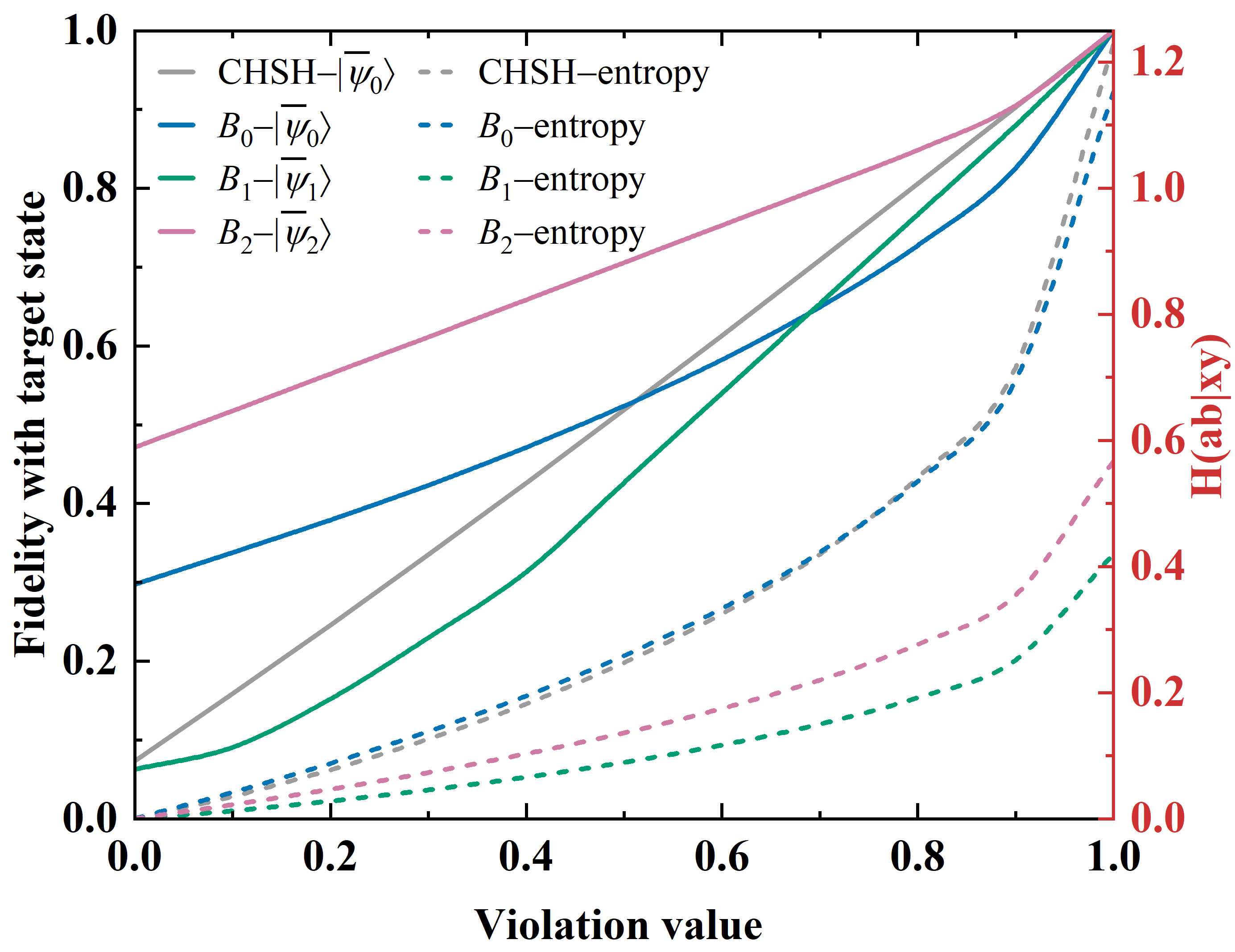
Figure 4: The lower bounds of fidelity with target state (left vertical axis) and randomness entropy (right vertical axis) with respect to the observation of Bell inequality. We denote $B_{[\alpha_{i},\beta_{i}]}$ as $B_{i}$ for $i=0,1,2$. The observed violation is made a transform $V_{i}=\frac{obs-C_{[\alpha_{i},\beta_{i}]}}{\eta_{[\alpha_{i},\beta_{i}]}-C_{[\alpha_{i},\beta_{i}]}}$. The fidelity with Bell state $\ket{\overline{\psi}_{0}}$ using standard CHSH and biased form are presented in gray and blue purple solid lines, respectively. The fidelity with $\ket{\overline{\psi}_{1}}$ and $\ket{\overline{\psi}_{2}}$ are represented in green and purple solid lines, respectively. The randomness for each Bell inequality is plotted with right vertical axis in dash color lines.

So far, we have provided the scheme that self-test different entangled states by fixed measurements settings based on generalized tilted-CHSH inequality, which is robust in tolerance of noise. Next, we demonstrate the applications of our results to simplify the implementations of secure quantum information tasks such as quantum key distribution (QKD), quantum random number generation (QRNG) and quantum private query (QPQ).

IV Applications in quantum information tasks

Quantum systems with self-testing property play important roles in quantum information processing. Especially, for the protocols which require a high demand for the security, self-testing is able to guarantee the security independently with the devices. This is precisely the fact that motivates the device independent (DI) quantum information processing. In last few years, the DI technologies have been studied intensively. Among of them, QKD, QRNG and QPQ as the core and bases of quantum cryptography, have gained huge attentions.

IV.1 Device independent quantum key distribution and private query

DIQKD allows distant parties to create and share a cryptographic key, whose security relies only on the certification of nonlocal quantum correlations DIQKD2014 . In the simplest protocol, entangled particles are repeatedly prepared and distributed between two parties, Alice and Bob. Alice holds two measurements $A_{x}$ for $x\in\{0,1\}$, Bob has three measurements $B_{y}$, $y\in\{0,1,2\}$. To ensure the security of the task, Alice and Bob perform CHSH test by randomly choosing two measurements $A_{x}$ and $B_{y}$, $x,y\in\{0,1\}$ respectively to certify the source device independently. The maximal quantum bound $2\sqrt{2}$ implies that the source is the maximum entangled state $\ket{\overline{\psi}}=\frac{1}{\sqrt{2}}(\ket{00}+\ket{11})$ and measurements are $A_{0}=\sigma_{z},A_{1}=\sigma_{x}$, $B_{0}=\frac{\sigma_{x}+\sigma_{z}}{\sqrt{2}}$ and $B_{1}=\frac{\sigma_{x}-\sigma_{z}}{\sqrt{2}}$. Then the measurement $A_{0}$ for Alice and the last one $B_{2}=\sigma_{z}$ for Bob are used to extract secure key.

Later motivated by this idea, a DIQPQ protocol was proposed in Ref. Maitra2017 . In the protocol, Alice and Bob share an entangled state with $\frac{1}{\sqrt{2}}(\ket{0}_{A}\ket{\phi_{0}}_{B}+\ket{1}_{A}\ket{\phi_{1}}_{B})$ where

$$\ket{\phi_{0}}_{B}=\cos\frac{\theta}{2}\ket{0}+\sin\frac{\theta}{2}\ket{1},$$

$$\ket{\phi_{1}}_{B}=\cos\frac{\theta}{2}\ket{0}-\sin\frac{\theta}{2}\ket{1}.$$ (21)

Before the process of QPQ Yang2014 , Alice and Bob perform a CHSH-like test to certify the source and measurements, which guarantee the measurements for Alice are in the basis $\{\ket{0},\ket{1}\}$ and $\{\ket{+},\ket{-}\}$, and Bob’s are in basis $\{\ket{\psi_{0}},\ket{\psi_{0}^{\perp}}\}$ or $\{\ket{\psi_{1}},\ket{\psi_{1}^{\perp}}\}$. If the outcome for Bob is $\ket{\psi_{0}^{\perp}}(\ket{\psi_{1}^{\perp}})$, he can conclude that the raw key bit at Alice must be 0(1). Bob and Alice execute classical post processing, so that information of Bob on the key reduces to one bit or more. Alice knows the whole key, whereas Bob generally knows several bits of the key.

According to our work, the measurements for Alice and Bob in above two protocols can be set as

$$A_{0} =\sigma_{z}\;B_{0}=\cos 2\theta\sigma_{z}+\sin 2\theta\sigma_{x},\;$$

$$A_{1} =\sigma_{x}\;B_{1}=\cos 2\theta\sigma_{z}-\sin 2\theta\sigma_{x},\;$$ (22)

which are available to self-test the two entangle sources in DIQKD and DIQPQ tasks at same time. For instance, the parameters in Eq. (4) can be set according to the task, i.e., $\alpha=\frac{1}{\tan 2\theta}$ and $\beta=0$ for DIQKD protocol, $\alpha=1$ and $\beta=\frac{2\cos\theta}{\sqrt{1+\sin^{2}\theta}}$ for DIQPQ protocol. In this way, different entangled states can not only be certified as the source in QKD, but also be used to generate secure key in QPQ task. This simplifies the measurement resources to achieve different quantum information processing.

IV.2 Device independent quantum random number generation

DIQRNG is able to access randomness by observing the violation of Bell inequalities without any assumptions on the source and measurement device. The randomness of the output pairs conditioned on the input pairs for the entangled pairs can be quantified by the min-entropy DIQRNG2010 $H_{\infty}(ab|xy)=-\log_{2}\max p(ab|xy)$. For a given observed violation $V_{i}$ of Bell inequality $B_{[\alpha_{i},\beta_{i}]}$, where $V_{i}$ is defined in the caption of Fig. 4, we are able to obtain a lower bound on the min-entropy

$$H_{\infty}(ab|xy)\geq V_{i}$$ (23)

satisfied by all quantum realizations of the Bell scenario. Let $P^{*}(ab|xy)$ denote the solution to the following optimization problem

obj $$P^{*}(ab|xy)=\max p(ab|xy)$$

s.t. $$\Gamma\geq 0,$$

$$\mathcal{B}_{[\alpha_{i},\beta_{i}]}=\text{observed violation value}\;\;i=0,1,2$$

where the optimization is carried over all states $\rho$ and all measurement operators, defined over Hilbert spaces of arbitrary dimension. The minimal value of the min-entropy compatible with the Bell violation $V$ and quantum theory is then given by $H_{\infty}(ab|xy)=-\log_{2}\max_{ab}P(ab|xy)$.

Using the same Bell inequalities in Sec. III and running SDP with NPA hierarchy, we plot the lower bounds of the entropy as shown in Fig. 4 with right vertical axis. It is noteworthy to point that in a device independent framework, if the violation is maximal quantum bound for CHSH $2\sqrt{2}$, the randomness is obtained with 1.2283 bits and the underlying structure is Bell state with orthogonal basis DIQRNG2010 . Here, we shown that if the two observers self-test the state with the biased basis as Eq. (II.2), the lower bound of randomness is 1.1519 bits, which is slightly lower than the CHSH scenario. However, we point out with this biased basis, the random numbers can also be certified from partially entangled states. As to the two partially entangled target states whose concurrence are respective $C(\ket{\overline{\psi}_{1}})=\frac{3}{4}$ and $C(\ket{\overline{\psi}_{2}})=\frac{\sqrt{3}}{2}\approx 0.866$, the secure randomness can be extracted with 0.4195 bits and 0.5669 bits, respectively. In other words, with this measurement settings, we can extract randomness in both the maximum entangled and partially entangled states.

V Conclusion

Self-testing results are usually known for a set of quantum state and corresponding measurement simultaneously. However different entangled resources are needed for various quantum information tasks with diverse requirements. In this paper we proposed a scheme that self-tests a family of entangled states with different entanglement degree by the same fixed measurement settings. By providing the SOS decompositions of generalized tilted-CHSH inequality, we extend the self-testing criteria of general two-qubit states with two binary measurements per party. The previous work based on symmetric biased CHSH Lawson2010 and standard tilted-CHSH operators 2015Bamps can be regarded as special cases of this criteria.The self-testing criteria obtained in our work are appealing from two aspects. For general two-qubit entangled states, we broaden its self-testing criteria. The self-testing can be carried out with a series of different measurements settings on Pauli $x$-$z$ plane, by setting different values of $\alpha$ in generalized tilted-CHSH inequality. More importantly, different entangled states can be self-tested by maximally violating corresponding Bell inequalities with the same fixed measurement settings. This can simplify the measurement instruments of self-testing in experimental realization. Moreover our scheme demonstrate satisfactory robustness in tolerance of noise.

Furthermore, our scheme can provide secure certification for different device-independent quantum information processing tasks with fewer resource. This work is instrumental to improve the practical performance of self-testing. In addition, this work is of intrinsic interest to the foundational studies on Bell nonlocality and quantum certification. In the future, it is interesting to study more Bell nonlocalities with self-testing property and find more criteria with the same measurements for different states.

Appendix. The SOS decomposition for generalized tilted-CHSH inequality

We provide the way to obtain the SOS decompositions of generalized tilted-CHSH operator (A.1)

$$\mathcal{B}_{[\alpha,\beta]}=\beta A_{0}+\alpha A_{0}B_{0}+\alpha A_{0}B_{1}+A_{1}B_{0}-A_{1}B_{1}$$ (A.1)

where $\alpha\geq 1$, in detail.

The optimal quantum violation of (A.1) is proved to be $\eta_{[\alpha,\beta]}=\sqrt{(1+\alpha^{2})(4+\beta^{2})}$ by optimizing over all quantum states and measurements Acin2012 . The bound implies the operator $\widehat{\mathcal{B}}=\eta_{[\alpha,\beta]}\mathbb{I}-\mathcal{B}_{[\alpha,\beta]}$ is positive semidefinite for all possible quantum states and measurement operators $A_{x}$ and $B_{y}$. This in turn can be proven by providing a set of operators $\{P_{i}\}$ which are polynomial functions of $A_{x}$ and $B_{y}$ such that

$$\widehat{\mathcal{B}}_{[\alpha,\beta]}=\sum_{i}P^{\dagger}_{i}P_{i}$$ (A.2)

holds for any set of measurement operators satisfying the algebraic properties $A^{2}_{x}=\mathbb{I}$, $B^{2}_{y}=\mathbb{I}$ and $[A_{x},B_{y}]=0$. The form (A.2) is called a SOS decomposition.

Our goal is to find SOS decompositions of generalized tilted-CHSH inequalities as in Eq. (A.2) in terms of a set of polynomials $\{P_{i}\}$. Our techniques on SOS decompositions is based on Ref. 2015Bamps . For simplicity, the search space is restricted to the span of a canonical basis of nine monomials

$$\mathcal{S}_{1+AB}=\{\mathbb{I},A_{0},A_{1}\}\otimes\{\mathbb{I},B_{0},B_{1}\}.$$ (A.3)

Let $\{R_{i}\}_{i}$ denote the different bases of the vector space of polynomial $P_{i}$. So $P_{i}$ can be expressed by bases $P_{i}=\sum_{\mu}q^{\mu}_{i}R_{\mu}$. The $\widehat{\mathcal{B}}$ is rewritten as

$$\widehat{\mathcal{B}}=\sum_{\mu v}\sum_{i}R^{\dagger}_{\mu}q^{\mu}_{i}q^{v}_{i}R_{v}=\sum_{\mu v}R^{\dagger}_{\mu}M^{\mu v}R_{v}.$$ (A.4)

The task turns to find a positive semidefinite matrix $M$ such that Eq. (A.4) holds. By decomposing both sides of the equality $\widehat{\mathcal{B}}=\sum_{\mu v}M^{\mu v}R^{\dagger}_{\mu}R_{v}$ in a basis of the quadratic products of all elements in $S_{1+AB}$, we obtain a canonical basis with size 25 for these products as

$$S^{2}_{1+AB}= \{\mathbb{I},A_{0},A_{1},A_{0}A_{1},A_{1}A_{0}\}$$

$$\otimes\{\mathbb{I},B_{0},B_{1},B_{0}B_{1},B_{1}B_{0}\}.$$ (A.5)

Writing $R^{\dagger}_{\mu}R_{v}=F^{i}_{\mu v}E_{i}$, where $E_{i}$ takes over $S^{2}_{1+AB}$ and each $F_{i}$ is a matrix of coefficients such that $\widehat{\mathcal{B}}=s^{i}E_{i}$. Then the SOS condition reduces to

$$s^{i}=Tr(M^{\dagger}F_{i})\text{ for }i=1,2,...,25.$$ (A.6)

The left thing is to solve a set of 25 linear equality constraints on $M$ as well as the positive semidefiniteness constraint $M\geq 0$.

A valid SOS decomposition for $\widehat{\mathcal{B}}_{[\alpha,\beta]}$ must be made up of terms for which $P_{i}(\cos\theta\ket{00}+\sin\theta\ket{11})$ vanishes in this maximally violating quantum system. Indeed, writing the most general $P$ in the search space as $r\cdot\mathbf{V}$ where

$$\mathbf{V}=(\mathbb{I},A_{0},A_{1},B_{0},B_{1},A_{0}B_{0},A_{0}B_{1},A_{1}B_{0},A_{1}B_{1}),$$ (A.7)

and demand the four components of $P_{i}\ket{\psi}$ vanish, Ref. 2015Bamps has shown that for $\alpha=1$ the space of candidates $P_{i}$ is spanned by the following five operators:

$$-Z_{A}+Z_{B}$$

$$-\mathbb{I}+Z_{A}Z_{B}$$

$$-\mathbb{I}+cZ_{B}+X_{A}X_{B}$$

$$-X_{A}+sX_{B}+cX_{A}Z_{B}$$

$$-cX_{A}+sZ_{A}X_{B}+X_{A}Z_{B}$$ (A.8)

where $c=\cos 2\theta$, $s=\sin 2\theta$ and operators $Z$ and $X$ are defined as

$$Z_{A}=A_{0},\; Z_{B}=\frac{B_{0}+B_{1}}{2\cos\mu},$$

$$X_{A}=A_{1},\; X_{B}=\frac{B_{0}-B_{1}}{2\sin\mu}.$$ (A.9)

We express the maximal violation of the generalized tilted-CHSH operator (A.1) with $\alpha$ and $\theta$

$$\eta_{[\alpha,\theta]}=\frac{2(\alpha^{2}+1)}{\sqrt{\alpha^{2}+\sin^{2}2\theta}}$$ (A.10)

which only be achieved by the state $\ket{\psi}=\cos\theta\ket{00}+\sin\theta\ket{11}$ and corresponding measurements $A_{x}$ and $B_{y}$ for $x,y\in\{0,1\}$ defined as (Appendix. The SOS decomposition for generalized tilted-CHSH inequality) and parameters satisfy

$$\beta=\frac{2\cos 2\theta}{\sqrt{\alpha^{2}+\sin^{2}2\theta}},$$

$$\cos\mu=\frac{\alpha}{\sqrt{\alpha^{2}+\sin^{2}2\theta}},$$ (A.11)

$$\sin\mu=\frac{\sin 2\theta}{\sqrt{\alpha^{2}+\sin^{2}2\theta}}.$$

Now we choose the basis ${R_{i}}=\{r_{i}\cdot\mathbf{V}\}$ for the subspace containing the SOS polynomials for generalized tilted-CHSH (A.1), and label the columns with the operators defining $\mathbf{V}$, where the $r_{i}$ vectors are defined as such

$$\begin{array}[]{ccccccccccc}&\mathbb{I}&A_{0}&A_{1}&B_{0}&B_{1}&A_{0}B_{0}&A_{0}B_{1}&A_{1}B_{0}&A_{1}B1&\\ r_{1}=(&0&-\frac{2\alpha}{\sqrt{\alpha^{2}+s^{2}}}&0&1&1&0&0&0&0&)\\ r_{2}=(&-\frac{2\alpha}{\sqrt{\alpha^{2}+s^{2}}}&0&0&0&0&1&1&0&0&)\\ r_{3}=(&-\frac{2}{\sqrt{\alpha^{2}+s^{2}}}&0&0&\frac{c}{\alpha}&\frac{c}{\alpha}&0&0&1&-1&)\\ r_{4}=(&0&0&-\frac{2}{\sqrt{\alpha^{2}+s^{2}}}&1&-1&0&0&\frac{c}{\alpha}&\frac{c}{\alpha}&)\\ r_{5}=(&0&0&-\frac{2c}{\sqrt{\alpha^{2}+s^{2}}}&0&0&1&-1&\frac{1}{\alpha}&\frac{1}{\alpha}&)\\ \end{array}$$ (A.12)

These basis operators separate the space in two isotypical subspaces, i.e., subspaces that fall under the same irreducible representation of the cyclic group: $R_{1,2,3}$ are invariant under the symmetry transformation of $\mathcal{B}_{[\alpha,\beta]}$, while $R_{4,5}$ change sign. The block structure of symmetric SOS matrices is therefore $3\oplus 2$, where the first block corresponds to the trivial representation and the second to the parity representation where the group generator is represented by $-1$.

For convenience, we define three classes CHSH operators:

$$S_{0} =A_{0}(B_{0}-B_{1})+\frac{1}{\alpha}A_{1}(B_{0}+B_{1}),$$

$$S_{1} =\frac{1}{\alpha}A_{0}(B_{0}+B_{1})-A_{1}(B_{0}-B_{1}),$$ (A.13)

$$S_{2} =A_{0}(B_{0}-B_{1})-\alpha A_{1}(B_{0}+B_{1}).$$

Then we can provide two different SOS decompositions of the generalized CHSH-inequalities $\mathcal{B}_{[\alpha,\beta]}$ in Eq. (A.1). The first one can be given as

$$\widehat{\mathcal{B}}_{[\alpha,\beta]}= \frac{1}{\Delta+2\eta_{[\alpha,\beta]}}\big{\{}(\alpha^{2}-1)\big{(}(\frac{\cos 2\theta}{\alpha}R_{1}-R_{3})^{2}+R_{1}^{2}\big{)}+\big{(}\frac{\cos 2\theta}{\alpha}R_{1}-\alpha R_{2}-R_{3}\big{)}^{2}+\alpha^{2}R_{5}^{2}\big{\}}$$

$$= \frac{1}{\Delta+2\eta_{[\alpha,\beta]}}\big{\{}(\alpha^{2}-1)[(-\beta A_{0}+\frac{\eta_{[\alpha,\beta]}}{\alpha^{2}+1}-A_{1}(B_{0}-B_{1}))^{2}$$

$$+(-\frac{\eta_{[\alpha,\beta]}\alpha}{\alpha^{2}+1}A_{0}+B_{0}+B_{1})^{2}]+\big{(}\eta_{[\alpha,\beta]}-\beta A_{0}-\alpha A_{0}(B_{0}+B_{1})-A_{1}(B_{0}-B_{1})\big{)}^{2}+\alpha^{2}R_{5}^{2}\big{\}}$$

$$= \frac{1}{\Delta+2\eta_{[\alpha,\beta]}}\{(\alpha^{2}-1)[({\color[rgb]{0,0,0}-}\beta A_{0}+\frac{\eta_{[\alpha,\beta]}}{\alpha^{2}+1}-A_{1}(B_{0}-B_{1}))^{2}+(-\frac{\alpha\eta_{[\alpha,\beta]}}{\alpha^{2}+1}A_{0}+B_{0}+B_{1})^{2}]$$

$$+\widehat{\mathcal{B}}_{[\alpha,\beta]}^{2}+\alpha^{2}(\beta A_{1}-(A_{0}(B_{0}-B_{1})+\frac{1}{\alpha}A_{1}(B_{0}+B_{1})))^{2}\}$$

$$= \frac{1}{\Delta+2\eta_{[\alpha,\beta]}}\{(\alpha^{2}-1)[({\color[rgb]{0,0,0}-}\beta A_{0}+\frac{\eta_{[\alpha,\beta]}}{\alpha^{2}+1}-A_{1}(B_{0}-B_{1}))^{2}+(-\frac{\eta_{[\alpha,\beta]}\alpha}{\alpha^{2}+1}A_{0}+B_{0}+B_{1})^{2}]$$

$$+\widehat{\mathcal{B}}_{[\alpha,\beta]}^{2}+\alpha^{2}(\beta A_{1}-S_{0})^{2}\}$$ (A.14)

where $\Delta=2(\alpha^{2}-1)\sqrt{\frac{\beta^{2}+4}{\alpha^{2}+1}}$. The second decomposition is given as

$$\widehat{\mathcal{B}}_{[\alpha,\beta]}= \frac{\alpha^{2}}{\Delta+2\eta_{[\alpha,\beta]}}\big{\{}\frac{\alpha^{2}-1}{\alpha^{2}}[(\frac{\cos 2\theta}{\alpha}R_{1}-R_{3})^{2}+R_{1}^{2}]+\big{(}\frac{2(\alpha^{2}+1)}{\alpha\eta_{[\alpha,\beta]}}R_{1}-\frac{\beta}{2}(\frac{1}{\alpha}R_{2}-R3)\big{)}^{2}+\frac{1}{{\color[rgb]{0,0,0}\alpha^{2}}}\big{(}\frac{\eta_{[\alpha,\beta]}}{2}R_{4}-\frac{\beta}{2}R_{5}\big{)}^{2}\big{\}}$$

$$= \frac{\alpha^{2}}{\Delta+2\eta_{[\alpha,\beta]}}\big{\{}\frac{\alpha^{2}-1}{\alpha^{2}}[({\color[rgb]{0,0,0}-}\beta A_{0}+\frac{\eta_{[\alpha,\beta]}}{\alpha^{2}+1}-A_{1}(B_{0}-B_{1}))^{2}+(-\frac{\alpha\eta_{[\alpha,\beta]}}{\alpha^{2}+1}A_{0}+B_{0}+B_{1})^{2}]$$

$$+\big{(}2A_{0}-\frac{\eta_{[\alpha,\beta]}}{2\alpha}(B_{0}+B_{1})+\frac{\beta}{2}(\frac{1}{\alpha}A_{0}(B_{0}+B_{1})-A_{1}(B_{0}-B_{1})))^{2}$$

$$+\frac{1}{{\color[rgb]{0,0,0}\alpha^{2}}}(2A_{1}-\frac{\eta_{[\alpha,\beta]}}{2}(B_{0}-B_{1})+\frac{\beta}{2}(A_{0}(B_{0}-B_{1})-\alpha A_{1}(B_{0}+B_{1})))^{2}\big{\}}$$

$$= \frac{\alpha^{2}}{\Delta+2\eta_{[\alpha,\beta]}}\big{\{}\frac{\alpha^{2}-1}{\alpha^{2}}[(-\frac{\eta_{[\alpha,\beta]}\alpha}{\alpha^{2}+1}A_{0}+B_{0}+B_{1})^{2}+({\color[rgb]{0,0,0}-}\beta A_{0}+\frac{\eta_{[\alpha,\beta]}}{\alpha^{2}+1}-A_{1}(B_{0}-B_{1}))^{2}]$$

$$+\big{(}2A_{0}-\frac{\eta_{[\alpha,\beta]}}{2\alpha}(B_{0}+B_{1})+\frac{\beta}{2}S_{1})^{2}+\frac{1}{{\color[rgb]{0,0,0}\alpha^{2}}}(2A_{1}-\frac{\eta_{[\alpha,\beta]}}{2}(B_{0}-B_{1})+\frac{\beta}{2}S_{2})^{2}\big{\}}$$ (A.15)

here $\Delta$ is defined as same in (Appendix. The SOS decomposition for generalized tilted-CHSH inequality)

Hence, we complete the SOS decompositions for $\widehat{\mathcal{B}}_{[\alpha,\beta]}$ such that $\widehat{\mathcal{B}}_{[\alpha,\beta]}=\sum_{i}P^{\dagger}_{i}P_{i}$ and $P_{i}$ are the polynomial functions of $A_{x}$ and $B_{y}$. The existence of SOS decompositions (Appendix. The SOS decomposition for generalized tilted-CHSH inequality) and (Appendix. The SOS decomposition for generalized tilted-CHSH inequality) implies that any state $\ket{\psi}$ and operators $A_{x}$ and $B_{y}$ achieving the maximal quantum bound $\eta_{[\alpha,\beta]}$ will result in $P_{i}\ket{\psi}=0$. Particularly, we are interested in the following four terms

$$P1\ket{\psi} =\widehat{\mathcal{B}}_{[\alpha,\beta]}\ket{\psi}$$ (A.16a)

$$P2\ket{\psi} =(\beta A_{1}-S_{0})\ket{\psi}$$ (A.16b)

$$P3\ket{\psi} =(2A_{0}-\frac{\eta_{[\alpha,\beta]}}{2\alpha}(B_{0}+B_{1})+\frac{\beta}{2}S_{1})\ket{\psi}$$ (A.16c)

$$P4\ket{\psi} =(2A_{1}-\frac{\eta_{[\alpha,\beta]}}{2}(B_{0}-B_{1})+\frac{\beta}{2}S_{2})\ket{\psi}$$ (A.16d)

which can be linearly combined to form the following operators

$$(Z_{A}-Z_{B})\ket{\psi} =0,$$ (A.17a)

$$(\sin\theta X_{A}(\mathbb{I}+Z_{B})-\cos\theta X_{B}(\mathbb{I}-Z_{A}))\ket{\psi} =0,$$ (A.17b)

in the case of yielding the maximal quantum bound. The algebraic relations (A.17a)–(A.17b) established by the SOS decompositions (Appendix. The SOS decomposition for generalized tilted-CHSH inequality)–(Appendix. The SOS decomposition for generalized tilted-CHSH inequality) are necessarily satisfied by any quantum state and observables achieving the maximal quantum bound. Moreover, they are important for the self-testing of partially entangled states $\ket{\psi}=\cos\theta\ket{00}+\sin\theta\ket{11}$ using the isometry circuit.

References

- [1] J. F. Clauser, M. A. Horne, A. Shimony, and R. A. Holt, Proposed experiment to test local hidden-variable theories. Phys. Rev. Lett. 23, 880–884 (1969).
- [2] N. Brunner, D. Cavalcanti, S. Pironio, V. Scarani, and S. Wehner, Bell nonlocality. Rev. Mod. Phys. 86, 419–478 (2014).
- [3] A. Acín, et al. Device-independent security of quantum cryptography against collective attacks. Phys. Rev. Lett. 98, 230501 (2007).
- [4] U. Vazirani, and T. Vidick, Fully Device-Independent Quantum Key Distribution. Phys. Rev. Lett. 113, 140501 (2014).
- [5] S. Pironio, et. al., Random numbers certified by Bell’s theorem. Nature 464, 1021–1024 (2010).
- [6] Y. Liu, et. al., Device-independent quantum random-number generation. Nature 562, 548–551 (2018).
- [7] T. Moroder, J.-D. Bancal, Y.-C. Liang, M. Hofmann, and O. Gühne, Device-independent entanglement quantification and related applications. Phys. Rev. Lett. 111, 030501 (2013).
- [8] J. Bowles, I. Šupić, D. Cavalcanti, and A Acín, Device-independent entanglement certification of all entangled states. Phys. Rev. Lett. 121, 180503 (2018).
- [9] D. Mayers, and A. Yao, Self testing quantum apparatus, Quantum Inf. Comput. 4, 273 (2004).
- [10] V. Scarani, The device-independent outlook on quantum physics, Acta Phys. Slovaca 62, 347–409 (2012).
- [11] I. Šupić, and J. Bowles, Self-testing of quantum systems: a review. Quantum 4, 337 (2020).
- [12] J. Barrett, and N. Gisin, How much measurement independence is needed to demonstrate nonlocality? Phys. Rev. Lett. 106, 100406 (2011).
- [13] S. Popescu, and D. Rohrlich, Which states violate Bell’s inequality maximally? Phys. Lett. A 169(6):411–414 (1992).
- [14] C. Bamps, and S. Pironio, Sum-of-squares decompositions for a family of Clauser-Horne-Shimony-Holt-like inequalities and their application to self-testing. Phys. Rev. A 91(5), 052111 (2015).
- [15] A. Coladangelo, K. T. Goh, and V. Scarani, All pure bipartite entangled states can be self-tested. Nat. Commun. 8, 15485 (2017).
- [16] X. Wu, J. D. Bancal, M. Mckague, and V. Scarani, Device-independent parallel self-testing of two singlets. Phys. Rev. A 93(6), 062121 (2016).
- [17] Y. Wang, X. Wu, and V. Scarani, All the self-testings of the singlet for two binary measurements. New J. Phys. 18(2), 025021 (2016).
- [18] M. McKague, Self-testing graph states, Conference on Quantum Computation, Communication, and Cryptography. Springer, Berlin, Heidelberg, 2011: 104–120.
- [19] X. Wu, C. Yu, T. H. Yang, H. N. Le, and V. Scarani, Robust self-testing of the three-qubit W state. Phys. Rev. A 90(4), 042339 (2014).
- [20] X. Li, Y. Cai, Y. Han, Q. Wen, and V. Scarani, Self-testing using only marginal information. Phys. Rev. A 98, 052331 (2018).
- [21] X. Li, Y. Wang, Y. Han, S. Qin, F. Gao, and Q. Wen, Self-testing of symmetric three-qubit states. IEEE J. Sel. Areas Commun. 38(3), (2020).
- [22] J. Kaniewski, Analytic and nearly optimal self-testing bounds for the Clauser-Horne-Shimony-Holt and Mermin inequalities. Phys. Rev. Lett. 117(7), 070402 (2016).
- [23] X. Li, Y.Wang, Y. Han, S. Qin, and F. Gao, Analytic robustness bound for self-testing of the singlet with two binary measurements. J. Opt. Soc. Am. B 36(2): 457–463 (2019).
- [24] T. Coopmans, J. Kaniewski, and C. Schaffner, Robust self-testing of two-qubit states. Phys. Rev. A 99, 052123 (2019).
- [25] J. D. Bancal, M. Navascué, V. Scarani, T. Vértesi, and T. H. Yang, Physical characterization of quantum devices from nonlocal correlations. Phys. Rev. A 91, 022115 (2015).
- [26] X. Wu, J. D. Bancal, M. McKague, and V. Scarani, Device independent parallel self-testing of two singlets. Phys. Rev. A 93, 062121 (2016).
- [27] M. McKague, T. H. Yang, and V. Scarani, Robust self-testing of the singlet. J. Phys. A-math. Theor. 45, 455304 (2012).
- [28] A. Coladangelo, Parallel self-testing of (tilted) EPR pairs via copies of (tilted) CHSH and the magic square game. Quantum Info. Comput. 17:831–865 (2017).
- [29] M. Coudron and A. Natarajan. The parallel-repeated magic square game is rigid. arXiv:1609.06306 (2016).
- [30] M. McKague. Self-testing in parallel with CHSH. New J. Phys. 18, 045013 (2016).
- [31] Sebastian Wagner, Jean-Daniel Bancal, Nicolas Sangouard, and Pavel Sekatski, Device-independent characterization of quantum instruments,Quantum 4 243 (2020).
- [32] A. Acín, S. Massar, and S. Pironio, Randomness versus nonlocality and entanglement. Phys. Rev. Lett. 108, 100402 (2012).
- [33] T. Lawson, N. Linden, and S. Popescu, Biased nonlocal quantum games. arXiv:1011.6245 (2010).
- [34] M. Navascués, S. Pironio, and A. Acín, A convergent hierarchy of semidefinite programs characterizing the set of quantum correlations. New J. Phys. 10, 073013 (2008).
- [35] Y.-G. Yang, S.-J. Sun, P. Xu, and J. Tian, Flexible protocol for quantum private query based on B92 protocol. Quantum Inf. Process. 13, 805–813 (2014).
- [36] A. Maitra, G. Paul, and S. Roy, Device-independent quantum private query. Phys. Rev. A 95, 042344 (2017).