11email: {cyli, dong, fishern, dzhu}@wayne.edu
Coupling User Preference with External Rewards to Enable Driver-centered and Resource-aware EV Charging Recommendation
Abstract
Electric Vehicle (EV) charging recommendation that both accommodates user preference and adapts to the ever-changing external environment arises as a cost-effective strategy to alleviate the range anxiety of private EV drivers. Previous studies focus on centralized strategies to achieve optimized resource allocation, particularly useful for privacy-indifferent taxi fleets and fixed-route public transits. However, private EV driver seeks a more personalized and resource-aware charging recommendation that is tailor-made to accommodate the user preference (when and where to charge) yet sufficiently adaptive to the spatiotemporal mismatch between charging supply and demand. Here we propose a novel Regularized Actor-Critic (RAC) charging recommendation approach that would allow each EV driver to strike an optimal balance between the user preference (historical charging pattern) and the external reward (driving distance and wait time). Experimental results on two real-world datasets demonstrate the unique features and superior performance of our approach to the competing methods.
Keywords:
Actor critic Charging recommendation Electric vehicle (EV) User preference External reward.1 Introduction
Electric Vehicles (EVs) are becoming popular due to their decreased carbon footprint and intelligent driving experience over conventional internal combustion vehicles [9] in personal transportation tools. Meanwhile, the miles per charge of an EV is limited by its battery capacity, together with sparse allocations of charging stations (CSs) and excessive wait/charge time, which are major driving factors for the so-called range anxiety, especially for private EV drivers. Recently, developing intelligent driver-centered charging recommendation algorithms are emerging as a cost-effective strategy to ensure sufficient utilization of the existing charging infrastructure and satisfactory user experience [19, 17].
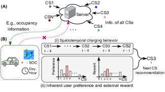
Existing charging recommendation studies mainly focus on public EVs (e.g., electric taxis and buses) [17, 2]. With relatively fixed schedule routines, and no privacy or user preference consideration, the public EV charging recommendation for public transits can be made completely to optimize CS resource utilization. In general, these algorithms often leverage a global server, which monitors all the CSs in a city (Fig. 1A). Charging recommendation can be fulfilled upon requests for public EVs by sending their GPS locations and state of charge (SOC). This kind of recommendation gives each EV an optimal driving and wait time before charging. Instead of using one single global server, many servers can be distributed across a city [1, 2] to reduce the recommendation latency for public EVs.
Although server-centralized methods have an excellent resource-aware property for the availability of charging for CSs, for private EVs, they rarely accommodate individual user preferences of charging and even have the risk of private data leakage (e.g., GPS location). Thus, the centralized strategy would also impair the trustworthiness [12, 6, 11] of the charging recommendation. A driver-centered instead of a server-centralized charging recommendation strategy would be preferred for a private EV to follow its user preference without leaking private information. In this situation (Fig. 1B), there would be a sequence of on-EV charging events records (when and which CS) that reflect the personal preference of charging patterns for a private EV driver. To enable the resource-aware property for a driver-centered charging recommendation, creating a public platform for sharing availability of CSs is needed.
Motivated by the success of recent research on the next POI (Point Of Interest) recommendation centered on each user, these studies can also be adapted to solve the charging recommendation problem for private EVs when viewing each CS as a POI. Different from collaborative filtering, based on the general recommendation that learns similarities between users and items [10], the following POI recommendation algorithms attempt to predict the most likely next POI that a user will visit based on the historical trajectory [23, 13, 26, 4, 24]. Although these methods indeed model user preferences, they are neither resource-aware nor adapted to the ever-changing external environment.
As such, a desirable charging recommender for a private EV requires: (1) learning the user preference from its historical charging patterns for achieving driver-centered recommendation, and (2) having a good external reward (optimal driving and wait time before charging) to achieve resource-aware recommendation (Fig. 1 B). By treating the private EV charging recommendation as the next POI recommendation problem, maximizing external rewards (with a shorter time of driving and wait before charging) by exploring possible CSs for each recommendation, reinforcement learning can be utilized. To leverage user preference and external reward, we propose a novel charging recommendation framework, Regularized Actor-Critic (RAC), for private EVs. The critic is based on a resource-saving over all CSs to give a evaluation value over the prediction of actor representing external reward, and the actor is reinforced by the reward and simultaneously regularized by the driver’s user preference. Both actor and critic are based on deep neural networks (DNNs).
We summarize the main contributions of this work as follows: (1) we design and develop a novel framework RAC to give driver-centered and resource-aware charging recommendations on-EV recommendation; (2) RAC is tailor-made for each driver, allowing each to accommodate inherent user preference and also adapt to ever-changing external reward; and (3) we propose a warm-up training technique to solve the cold-start recommendation problem for new EV drivers.
2 Related Work
Next POI recommendation has attracted much attention recently in location-based analysis. There are two lines of POI recommendation methods: (1) following user preference from sequential visiting POIs regularities, and (2) exploiting external incentive via maximizing the utility (reward) of recommendations.
For the first line of research, the earlier works primarily attempt to solve the sequential next-item recommendation problem using temporal features. For example, [13] introduces Factorizing Personalized Markov Chain (FPMC) that captures sequential dependency between the recent and next items as well as the general taste of a user using a combination of matrix factorization and Markov chains for next-basket recommendation. [26] proposes a time-related Long-Short Term Memory (LSTM) network to capture both long- and short-term sequential influence for next item recommendation. [5] attempts to model user’ preference drift over time to achieve a better user experience in next item recommendation. These next-item recommendation approaches only use temporal features whereas next POI recommendation would need to use both temporal and geospatial features.
More recent studies of next POI recommendation not only model temporal relations but also consider geospatial context, such as ST-RNN [7] and ATST-LSTM [3]. [4] proposes a hierarchical extension of LSTM to code spatial and temporal contexts into the LSTM for general location recommendation. [24] introduces a spatiotemporal gated network model where they leverage time gate and distance gate to control the effect of the last visited POI on next POI recommendation. [23] extends the gates with a power-law attention mechanism with more attention on the nearby POIs and explores the subsequence patterns for next POI recommendation. [21] develops a long and short-term preference learning model considering sequential and context information for next POI recommendation. User preference-based methods can achieve significant performance for the following users’ previous experience; however, they are restricted from making novel recommendations beyond users’ previous experience.
Although few studies exploit external incentive, these methods can help explore new possibilities for next POI recommendation. Charging Recommendation with multi-agent reinforcement learning is applied for public EVs[16, 22], in which private information from each EV is inevitably required. [8] proposes an inverse reinforcement learning method for next visit action recommendation by maximizing the reward that the user gains when discovering new, relevant, and non-popular POIs. This study utilizes the optimal POI selection policy (the POI visit trajectory of a similar group users) as the guidance. As such, it is only applicable for the centralized charging recommendation for privacy-indifferent public transit fleets where charging events are aggregated to the central server to learn the user group. However, this approach is not applicable to the driver-centered EV charging recommendation problem that we are tackling since the individual charging pattern is learned without data sharing across drivers. Besides the inverse reinforcement learning approach, [25] introduces deep reinforcement learning for news recommendation, and [18] proposes supervised reinforcement learning for treatment recommendation. These methods are also based on learning similar user groups thus not directly applicable to the driver-centered EV charging recommendation task, the latter is further subject to resource and geospatial constraints.
Despite the existing approaches utilized spatiotemporal, social network, and/or contextual information for effective next POI recommendations, they do not possess the desirable features for CS recommendation, which are (1) driver-centered: the trade-off between the driver’s charging preference and the external reward is tuned for each driver, particularly for new drivers, and (2) resource-aware: there is usually capacity constraint on a CS but not on a social check-in POI.
3 Problem Formulation
Each EV driver is considered as an agent, and the trustworthy server that collects occupancy information of all the CSs represent the external ever-changing environment. We considered our charging recommendation as a finite-horizon MDP problem where a stochastic policy consists of a state space , an action space , and a reward function : . At each time point , an EV driver with the current state , chooses an action , i.e., the one-hot encoding of a CS, based on a stochastic policy where is the set of parameters, and receives a reward from the spatiotemporal environment. Our objective is to learn such a stochastic policy to select an action by maximizing the sum of discounted rewards (return ) from the time point , which is defined as , and simultaneously minimizing the difference from the EV driver’s decision . , e.g., 0.99, is a discount factor to balance the importance of immediate and future rewards. is the furthermost time point we use.
The charging recommendation task is a process to learn a good policy for next CS recommendation for an EV driver. By modeling user behaviors with situation awareness, two types of methods can be designed to learn the policy: value based Reinforcement Learning (RL) to maintain a greedy policy, and policy gradient based RL to learn a parameterized stochastic policy or a deterministic policy , where represents the set of parameters of the policy. For the discrete property of CSs, we focus on learning a personalized stochastic policy for each EV driver using DNNs.
4 Our Approach
4.1 Background
Q-learning [20] is an off-policy learning strategy for solving RL problems that finds a greedy policy , where is value or action-value, and it is usually used for a small discrete action space. For any finite Markov decision process, Q-learning finds an optimal policy in the sense of maximizing the expected value of the total reward over any successive steps, starting from the current state. The value of can be calculated with dynamic programming. With the introduction of DNNs, a deep Q network (DQN) is used to learn such function with parameter , and DNN is incapable of handling a high dimension action space. During training, a replay buffer is introduced for sampling, and DQN asynchronously updates a target network to minimize the expectation of square loss.
Policy gradient [15] is another approach to solve RL problems and can be employed to handle continuous or high-dimensional discrete actions, and it targets modeling and optimizing the policy directly. The policy is usually modeled with a parameterized function respect to , . The value of the reward (objective) function depends on this policy and then various algorithms can be applied to optimize for the best reward. To learn the parameter of , we maximize the expectation of state-value function , where is the state-value function. Then we need to maximize , where represents the discounted state distribution. Policy gradient learns the parameter by the gradient , which is calculated with the policy gradient theorem: . These calculations are guaranteed by the policy gradient theorem.
Actor-critic [14] method combines the advantages of Q-learning and policy gradient to accelerate and stabilize the learning process in solving RL problems. It has two components: a) an actor to learn the parameter of in the direction of the gradient to maximize , and b) a critic to estimate the parameter in an action-value function .
In this paper, we use an off-policy actor-critic [14, 18], where the actor updates the policy weights. The critic learns an off-policy estimate of the value function for the current actor policy, different from the (fixed) behavior policy. The actor then uses this estimate to update the policy. Actor-critic methods consist of two models, which may optionally share parameters. Critic updates the value function parameters for state action-value . Actor updates the policy parameters for , in the direction suggested by the critic. is obtained by averaging the state distribution of behavior policy . for collecting samples is a known policy (predefined just like a hyperparameter). The objective function sums up the reward over the state distribution defined by this behavior policy: , where is the stationary distribution of the behavior policy ; and is the action-value function estimated with regard to the target policy .
4.2 The Regularized Actor-Critic (RAC) Method
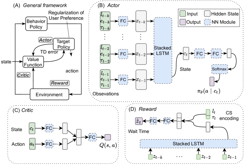
To find an optimal policy for the MDP problem also with following user preference, we use the regularized RL method, specifically with a regularized actor-critic model [18], which combines the advantages of Q-learning and policy gradient. Since the computation cost becomes intractable with many states and actions when using policy iteration and value iteration, we introduce a DNN-based actor-critic model to reduce the computation cost and stabilize the learning. While the traditional actor-critic model aims to maximize the reward without considering a driver’s preference, we also use regularization to learn the user’s historical charging behavior as a representation of user preference. Our proposed general regularized actor-critic framework is shown in Fig. 2A.
The actor network learns a policy with a set of parameters to render charging recommendation for each EV driver, where the input is and the output is the probabilities of all actions in of transitioning to a CS . By optimizing the two learning tasks simultaneously, we maximize the following objective function:
where is tuning parameter to weigh between inherent user preference and external reward (return) when making recommendation. The RL objective aims to maximize the expected return via learning the policy by maximizing the state value of an action that is averaged over the state distribution of the CS selection for each EV driver, i.e.,
The regularization objective aims to minimize the discrepancy between the recommended CS and preferred CS for each user via minimizing the difference between CS recommended by and CS given by each EV driver’s previous selection, in terms of the cross entropy loss, i.e.,
Using DNNs, can be learned with stochastic gradient decedent (SGD) algorithms.
The critic network is jointly learned with the actor network, where the inputs are the current and previous states (i.e., CSs) of each EV driver, actions, and rewards. The critic network uses a DNN to learn the action-value function , which is used to update the parameters of the actor in the direction of reward improvement. The critic network is only needed for guiding the actor during training whereas only actor network is required at test stage. We update the parameter via minimizing
in which , is the charging action recommended by the actor network, and is Temporal Difference (TD) error, which is used for learning the Q-function.
4.3 The RAC Framework for EV Charging Recommendation
In the previous formulation, we assume the state of an EV driver is fully observable. However, we are often unable to observe the full states of an EV driver. Here we reformulate the environment of RAC as Partially Observable Markov Decision Process (POMDP). In POMDP, is used to denote the observation set, and we obtain each observation directly from . For simplicity, we use a stacked LSTM together with the previous Fully Connected (FC) layers for each input step (Fig. 2B), to summarize previous observations to substitute the partially observable state with . Each represents a observation in different time points, and is the set of parameters of . denotes the CS location context information, presents charging event related features (e.g., SOC), and represents the time point (e.g., day of a week and hour of a day). is a combination context with the geodesic distance from previous CS (calculated by the latitudes and longitudes), one-hot encoding of this CS and the POI distribution around this CS. is a concatenation of , and vectors. The samples for training the actor model is generated from the behavior actor (i.e., from the real world charging trajectories) via a buffer in an off-policy setting.
Our RAC consists of three main DNN modules for estimating the actor, the critic, and the reward, as shown in Fig. 2. Actor DNN (Fig. 2B) captures each driver’s charging preference. We take a subsequence of the most recent CSs as input to extract the hidden state through a stacked-LSTM. With the following fully connected layers, we recommend the CS to go next for an EV driver. During training, the actor is supervised with the TD from the critic network to maximize the expected reward and the actual CS selection from this driver with cross-entropy loss to minimize the difference (Fig. 2A) . Since the actor is on each EV and takes private charging information as input, it is a driver-centered charging recommendation model.
To enable resource-awareness, we use a one-way information transmission scheme, shown in Fig. 1. We train a resource-aware actor for each EV driver via estimating value from the critic DNN with addition of the immediate reward estimated with a reward DNN. Fig. 2C shows the prediction of value of state and action , and the state here would be substituted with in POMDP setting. Fig. 2D describes how to estimate the wait time in all CSs. We can calculate the immediate reward for each pair of by combining with the estimated drive time. To tackle the cold start problem for new EV drivers, we introduce a warm-up training technique to update the model and will illustrate the details in the experiment section.
4.4 Timely Estimation of Reward
In stead of using traditional static reward, we dynamically estimate the reward from external environment. Since the drive time to and wait time at the CS play a key role for private EV driver’s satisfaction, we estimate rewards based on these two factors. Specifically, we directly use the geodesic distance from map to represent the drive time and use a DNN (Fig. 2D) to timely estimate the wait time for each charging. Therefore, a timely estimation of reward for choosing each CS can be given by a simple equation: where is the predicted wait time through reward network, in which is the parameters of the reward DNN (LSTM). is the wait time in steps before the current time step, and it is directly summarized from the dataset we used. is the estimated driving distance to the corresponding CS. Further, and represent statistically averaged driving distance and wait time in each CS, and they are constant values for a specific CS. is a coefficient, which usually has an inverse relationship with an EV driver’s familiarity with the routes (visiting frequency of each CS). For simplicity, we set as 0.8 for the most visited CS, and 1 for other situations. To make the predicted wait time and predicted driving distance to be additive, we do normalization for the predicted values by the averaged wait time and respectively for each CS. Since the wait time and drive time are estimated by each CS, our RAC framework is resource-aware to make CS recommendation for each EV driver.
Putting all the components as mentioned above together, the training algorithm of RAC is shown in Algorithm 1.
Input: Actions , observations , reward function , of CSs , historical wait time at each hour , and coordinates in -th CS
Hyper-parameters: Learning rate , , the finite-horizon step , number of episodes , and
Output:
4.5 Geospatial Feature Learning
The POI distribution within the neighborhood of each CS is what we used to learn the geospatial features from each CS. With this information, we can infer the semantic relationships among the CSs to assist in recommending CSs for each driver. Google Map defines 76 types (e.g., schools, restaurants, and hospitals) of POIs. Specifically, for each CS, we use its latitude and longitude information together with a geodesic radius of 600 meters to pull the surrounding POIs. We count the number of POIs for each type to obtain a 76-dimension vector (e.g., ) as the POI distribution. We concatenate this vector with other information, i.e., geodesic distances to CSs and one-hot encoding of the CS. With the charging event features and the timestamp-related features, we learn a unified embedding through an MLP for each input step of the stacked-LSTM.
5 Experiments
5.1 Experimental Setup
All the experiments are implemented on two real world charging events datasets from Dundee city 111https://data.dundeecity.gov.uk/dataset/ and Glasgow city 222http://ubdc.gla.ac.uk/dataset/. The POI distribution for each CS is obtained from Google Place API333https://developers.google.com/maps/documentation/places/web-service. The code of our method is publicly available on this link: https://github.com/cyli2019/RAC-for-EV-Charging-Rec.
5.1.1 Datasets and Limitations
For Dundee city, we select the charging events from the time range of 6/6/2018-9/6/2018, in which there are 800 unique EV drivers, 44 CSs and 19, 115 charging events. For Glasgow city, in the time range of 9/1/2013-2/14/2014, we have 47 unique EV drivers, 8 CSs and 507 charging events. For each charging event, the following variables are available: CS ID, charging event ID, EV charging date, time, and duration, user ID, and consumed energy (in kWh) for each transaction. For each user ID, we observe a sequence of charging events in chronological order to obtain the observations . For each CS ID, we learn the geospatial feature to determine their semantic similarity according to POI types.
To model an EV driver preference, we train a model using the CS at each time point as the outcome and the previous charging event sequence as the input. To enable situation awareness, for a specific CS, there is a chronically ordered sequence of wait time, and we use the wait time corresponding to each time point as the outcome and that of previous time points as inputs in our reward network to forecast hourly wait time for all CS’s. Combined with the estimated drive time that are inverse proportional to familiarity adjusted geodesic distance, we determine the timely reward for each EV driver’s charging event.
To our knowledge, these two datasets are the only publicly available driver-level charging event data for our driver-centered charging recommendation task, though with relatively small size and unavailability of certain information. Due to the privacy constraints, the global positioning system (GPS) information of each driver and the corresponding timestamp are not publicly available as well as traffic information in these two cities during the time frame. As such, we have no choice but having to assume the EV driver transits from CS to CS and using driving distance between CSs combined with estimated wait time at each CS to calculate the external reward. Another assumption we made is using the time interval of each charging event to approximate the SOC of the EV since all EVs in the data sets are of the same model. The method developed in this paper is general that does not rely on the aforementioned assumption; when GPS, timestamp and SOC information become available, our method is ready to work without change.
5.1.2 Evaluation Metrics
Similar to POI recommendation, we treat the earlier 80% sequences of each driver as a training set, the middle 10% as a validation set, and the latter 10% as a test set. Two standard metrics are adopted to evaluate methods’ performance, namely, Precision (P@K) and Recall (R@K) on the test set. To quantify the external reward for making a charging recommendation, we also use a Mean Average Reward (MAR) as an evaluation metric. Each reward is calculated based on familiarity-adjusted geodesic distance and projected wait time at the recommended CS, and MAR is the average value over all users across all time points in the test set. To solve the cold-start problem for EV drivers who have few charging events, we use 5% of data in the earlier sequences from all users (with more than 10 charging events) to train a model as warm-up, the rest 95% following the same data splitting strategy described above followed by training with each driver’s private data. We assume that for the earliest 5% of data can be shared without privacy issues when the user related information is eliminated.
| Dataset | Metrics | MC | FPMC | Time-LSTM | ST-RNN | ATST-LSTM | RAC-zero | RAC | Improvement |
|---|---|---|---|---|---|---|---|---|---|
| Dundee | @1 | 0.204 | 0.242 | 0.313 | 0.326 | 0.368* | 0.385 | 0.424 | 15.2% |
| @3 | 0.256 | 0.321 | 0.367 | 0.402 | 0.435* | 0.463 | 0.509 | 17.0% | |
| @5 | 0.321 | 0.363 | 0.436 | 0.437 | 0.484* | 0.528 | 0.577 | 19.2% | |
| @1 | 0.146 | 0.195 | 0.203 | 0.216 | 0.247* | 0.285 | 0.292 | 18.2% | |
| @3 | 0.153 | 0.226 | 0.236 | 0.278 | 0.298* | 0.344 | 0.368 | 23.5% | |
| @5 | 0.192 | 0.237 | 0.245 | 0.325 | 0.375* | 0.427 | 0.479 | 27.7% | |
| -327.8 | -265.9 | -210.4 | -195.4 | -164.5* | -133.2 | -114.6 | 30.3% | ||
| Glasgow | @1 | 0.163 | 0.207 | 0.264 | 0.252 | 0.294* | 0.313 | 0.364 | 23.8% |
| @3 | 0.226 | 0.262 | 0.325 | 0.356 | 0.375* | 0.40.9 | 0.458 | 22.1% | |
| @5 | 0.285 | 0.301 | 0.398 | 0.405 | 0.428* | 0.482 | 0.497 | 16.1% | |
| @1 | 0.108 | 0.093 | 0.122 | 0.128 | 0.133* | 0.13.1 | 0.164 | 23.3% | |
| @3 | 0.126 | 0.135 | 0.174 | 0.182 | 0.216* | 0.224 | 0.253 | 17.1% | |
| @5 | 0.173 | 0.167 | 0.263 | 0.323 | 0.334* | 0.395 | 0.406 | 21.5% | |
| -456.3 | -305.4 | -232.2 | -210.9 | -196.4* | -164.2 | -154.3 | 21.4% |
5.1.3 Baselines
We compare RAC with the following baseline methods, including two classic methods (i.e., MC, and FPMC [13]), three DNN-based state-of-the-art methods (i.e., Time-LSTM [26] , ST-RNN [7], and ATST-LSTM [3]). We select these methods as the baselines for method comparison, instead of other general POI recommendation methods (e.g., multi-step or sequential POI recommendation problem), because they directly address the next POI recommendation problem. One variant of our RAC (i.e., RAC-zero) is trained from scratch without warm-up training. The description of the baselines are: (1) MC: first-order Markov Chain utilizes sequential data to predict a driver’s next action based on the last actions via learning a transition matrix. (2) FPMC: Matrix factorization method learns the general taste of a driver by factorizing the matrix over observed driver-item preferences. Factorization Personalized Markov Chains model is a combination of MC and MF approaches for the next-basket recommendation. (3) Time-LSTM: Time-LSTM is a state-of-the-art variant of LSTM model used in recommender systems. Time-LSTM improves the modeling of sequential patterns by explicitly capturing the multiple time structures in the check-in sequence. We used the best-performing version reported in their paper. (4) ST-RNN : It is a RNN-based method that incorporates spatiotemporal contexts for next location prediction. (5) ATST-LSTM: It utilizes POIs and spatiotemporal contexts in a multi-modal manner for next POI prediction. In addition, to evaluate the effect of warm-up training on solving the cold-start problem, we compare our RAC with its a variant, RAC-zero, which is trained from scratch.
5.2 Performance Comparison
The parameter tuning information during the training are described above, and after that we make comparison for our approach with the baselines methods.Table 1 presents the performance (R@K, P@K, and MAR) of all methods across the two datasets. We test with 1, 3, and 5, and based on the parameter tuning results, we use the setting of two-layer stacked-LSTM for both actor and reward networks, embedding/hidden sizes of (100, 100), of 0.5, and learning rate of 0.001. The feeding steps for LSTMs in actor and reward networks are set to 5 and 10 respectively. In terms of charging recommendation task, the RNN based methods (Time-LSTM, ST-RNN, ATST-LSTM, and RAC) generally outperforms non-RNN based competitors (MC, and FPMC) owing to the leverage of spatiotemporal features. For the former, ATST-LSTM is better than ST-RNN possibly due to the effective use of attention mechanism. ST-RNN has slightly better performance over Time-LSTM due to the incorporation of spatial features. Overall, our proposed RAC consistently achieves the best performance not only on precision/recall but also over MAR, in which the improvement column are the comparisons between RAC and the runner-up model (ATST-LSTM). This is translated into the fact that overall RAC is capable of accommodating inherent user preference and ensuring the external rewards to a maximum extent in rendering charging recommendations.
To demonstrate the influence of warm-up training in RAC, we compare it with the training-from-scratch-approach RAC-zero. From Table 1, RAC demonstrates a better overall performance on the Dundee dataset for the relative abundance of samples for warm-up training; in the meanwhile, due to the limited number of warm-up training samples in the Glasgow dataset, this improvement is relatively slight. Conventionally, the Glasgow dataset with fewer charging stations might have better recommendation accuracy than the Dundee dataset. However, we should know that most (over 80%) EVs are revisiting no more than eight charging stations for both datasets. Therefore, for driver-centered charging pattern, the number of possible CSs is similar for these two datasets, resulting in even worse performance for the Glasgow dataset than the Dundee dataset. Overall, our proposed RAC consistently achieves the best performance not only on precision/recall but also over MAR.
5.3 Driver-centered CS Recommendation
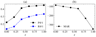
Fig. 3 illustrates the effect of personalization tuning parameter on precision/recall and reward of the recommendation. Since RAC is a driver-centered recommendation method, each driver can experiment with the parameter to weigh more on inherent user preference or on external award when seeking driver-centered charging recommendations. In Fig. 3A, the P@1 and R@1 of RAC climb up as increases, and becomes stable at around 0.5, indicating a larger value would not further improve the performance. In Fig. 3(b), MAR first decreases slightly before 0.5 and then drops quickly afterwards. Collectively, it appears an average driver can get the best of both worlds when is around 0.5.
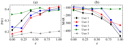
Fig. 4 shows that drivers 1-3 follow a very similar pattern to the average driver in Fig. 3 where is around 0.5, representing a good trade-off to balance between the inherent user preference and the external reward. Driver 4 represents a special case where the driver preference aligns well with the external reward; in this case the charging recommendation is invariant to the choice of . Hence the recommendation can be made either based on user preference or external reward since they are consistent to each other. Driver 5 represents a new driver with low precision and recall due to the lack of historical charging data. As such, the recommendation can simply be made based mostly on the external reward via setting to a low value, e.g., 0.2. In sum, tuning indeed enables an individual driver to be more attentive to his/her preference or to the external reward when seeking EV charging recommendation.
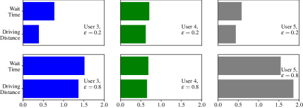
Fig. 5 demonstrates the award (e.g., wait time and driving distance) for three representative EV drivers, User 3, User 4, and User 5, under two different values of , i.e., 0.2 and 0.8. Recall the latter denotes the weight on an EV driver to follow historical charging pattern. Therefore, an increase of the value from 0.2 to 0.8 indicates that the charging recommendation is rendered based more on the driver’s previous charging pattern than the reward from external environment. In Fig. 5, we describe three types of drivers demonstrated by different trade-offs: (1) For User 3, the wait time and driving distance are both increasing, resulting in a smaller reward, whereas a better prediction accuracy. (2) For User 4, the wait time and driving distance remains shorter yet stable across the two values of , demonstrating both a larger reward and higher prediction accuracy. (3) For User 5 who is a newer driver, the reward increases similarly to User 3. However, the prediction accuracy stays low regardless of the choice of due to the limited information on historical charging pattern of the new driver. In summary, for drivers such as User 3 whose charging patterns are vastly deviated from what would be recommended by the external award, tuning would allow the drivers to be more attentive to either historical charging patterns or the external award. For drivers such as User 4 whose historical charging pattern is consistent with the more rewarding charging option as determined by shorter wait time and driving distance, the choice of does not matter, representing an optimal charging recommendation scenario. For new drivers such as User 5, a charging recommendation that is largely based on the external reward may be more appropriate.
6 Conclusion
In this paper, we propose a resource-aware and driver-centered charging recommendation method for private EVs. We devise a flexible regularized actor-critic framework, i.e., using RL to maximize external reward as the regularization to model inherent user preference for each driver. Our approach is sufficiently flexible for a wide range of EV drivers including new drivers with limited charging pattern data. Experimental results on real-world datasets demonstrate the superior performance of our approach over the state-of-the-arts in the driver-centered EV charging recommendation task.
Acknowledgements This work is supported by the National Science Foundation under grant no. IIS-1724227.
References
- [1] Cao, Y., Kaiwartya, O., Zhuang, Y., Ahmad, N., Sun, Y., Lloret, J.: A decentralized deadline-driven electric vehicle charging recommendation. IEEE Systems Journal (2018)
- [2] Guo, T., You, P., Yang, Z.: Recommendation of geographic distributed charging stations for electric vehicles: A game theoretical approach. In: 2017 IEEE Power & Energy Society General Meeting. pp. 1–5 (2017)
- [3] Huang, L., Ma, Y., Wang, S., Liu, Y.: An attention-based spatiotemporal lstm network for next poi recommendation. IEEE Transactions on Services Computing (2019)
- [4] Kong, D., Wu, F.: Hst-lstm: A hierarchical spatial-temporal long-short term memory network for location prediction. In: IJCAI. vol. 18, pp. 2341–2347 (2018)
- [5] Li, L., Zheng, L., Yang, F., Li, T.: Modeling and broadening temporal user interest in personalized news recommendation. Expert Systems with Applications 41(7), 3168–3177 (2014)
- [6] Li, X., Li, X., Pan, D., Zhu, D.: Improving adversarial robustness via probabilistically compact loss with logit constraints. In: AAAI. vol. 35, pp. 8482–8490 (2021)
- [7] Liu, Q., Wu, S., Wang, L., Tan, T.: Predicting the next location: A recurrent model with spatial and temporal contexts. In: AAAI. vol. 30 (2016)
- [8] Massimo, D., Ricci, F.: Harnessing a generalised user behaviour model for next-poi recommendation. In: RecSys ’18. pp. 402–406 (2018)
- [9] O’Donovan, C., Frith, J.: Electric buses in cities: Driving towards cleaner air and lower co 2. Bloomberg New Energy Finance, NY, USA, Tech. Rep (2018)
- [10] Pan, D., Li, X., Li, X., Zhu, D.: Explainable recommendation via interpretable feature mapping and evaluation of explainability. In: IJCAI. pp. 2690–2696 (2020)
- [11] Pan, D., Li, X., Zhu, D.: Explaining deep neural network models with adversarial gradient integration. In: IJCAI. pp. 2876–2883 (2021)
- [12] Qiang, Y., Li, C., Brocanelli, M., Zhu, D.: Counterfactual interpolation augmentation (cia): A unified approach to enhance fairness and explainability of dnn. In: IJCAI (2022)
- [13] Rendle, S., Freudenthaler, C., Schmidt-Thieme, L.: Factorizing personalized markov chains for next-basket recommendation. In: WWW’10. pp. 811–820 (2010)
- [14] Schmitt, S., Hessel, M., Simonyan, K.: Off-policy actor-critic with shared experience replay. In: ICML (2020)
- [15] Sutton, R.S., McAllester, D.A., Singh, S.P., Mansour, Y., et al.: Policy gradient methods for reinforcement learning with function approximation. In: NIPS. vol. 99, pp. 1057–1063 (1999)
- [16] Wang, E., Ding, R., Yang, Z., Jin, H., Miao, C., Su, L., Zhang, F., Qiao, C., Wang, X.: Joint charging and relocation recommendation for e-taxi drivers via multi-agent mean field hierarchical reinforcement learning. IEEE Transactions on Mobile Computing (2020)
- [17] Wang, G., Xie, X., Zhang, F., Liu, Y., Zhang, D.: bcharge: Data-driven real-time charging scheduling for large-scale electric bus fleets. In: RTSS. pp. 45–55 (2018)
- [18] Wang, L., Zhang, W., He, X., Zha, H.: Supervised reinforcement learning with recurrent neural network for dynamic treatment recommendation. In: KDD’18. pp. 2447–2456 (2018)
- [19] Wang, X., Yuen, C., Hassan, N.U., An, N., Wu, W.: Electric vehicle charging station placement for urban public bus systems. IEEE Transactions on Intelligent Transportation Systems 18(1), 128–139 (2016)
- [20] Watkins, C.J., Dayan, P.: Q-learning. Machine learning 8(3-4), 279–292 (1992)
- [21] Wu, Y., Li, K., Zhao, G., Qian, X.: Long-and short-term preference learning for next poi recommendation. In: CIKM’19. pp. 2301–2304 (2019)
- [22] Zhang, W., Liu, H., Wang, F., Xu, T., Xin, H., Dou, D., Xiong, H.: Intelligent electric vehicle charging recommendation based on multi-agent reinforcement learning. In: WWW’21. pp. 1856–1867 (2021)
- [23] Zhao, K., Zhang, Y., Yin, H., Wang, J., Zheng, K., Zhou, X., Xing, C.: Discovering subsequence patterns for next poi recommendation. In: IJCAI. pp. 3216–3222 (2020)
- [24] Zhao, P., Zhu, H., Liu, Y., Xu, J., Li, Z., Zhuang, F., Sheng, V.S., Zhou, X.: Where to go next: A spatio-temporal gated network for next poi recommendation. In: AAAI. vol. 33, pp. 5877–5884 (2019)
- [25] Zheng, G., Zhang, F., Zheng, Z., Xiang, Y., Yuan, N.J., Xie, X., Li, Z.: Drn: A deep reinforcement learning framework for news recommendation. In: WWW’18 (2018)
- [26] Zhu, Y., Li, H., Liao, Y., Wang, B., Guan, Z., Liu, H., Cai, D.: What to do next: Modeling user behaviors by time-lstm. In: IJCAI. vol. 17, pp. 3602–3608 (2017)