Infrared Spectroscopic Survey of the Quiescent Medium of Nearby Clouds: II. Ice Formation and Grain Growth in Perseus and Serpens

Abstract

The properties of dust change during the transition from diffuse to dense clouds as a result of ice formation and dust coagulation, but much is still unclear about this transformation. We present 2-20 $\mu$m spectra of 49 field stars behind the Perseus and Serpens Molecular Clouds and establish relationships between the near-infrared continuum extinction ($A_{\rm K}$) and the depths of the 9.7 $\mu$m silicate ($\tau_{9.7}$) and 3.0 $\mu$m $\rm{H_{2}O}$ ice ($\tau_{3.0}$) absorption bands. The $\tau_{9.7}$/$A_{\rm K}$ ratio varies from large, diffuse interstellar medium-like values ($\sim 0.55$), to much lower ratios ($\sim 0.26$). Above extinctions of $A_{\rm K}\sim 1.2$ ($A_{\rm V}\sim 10$; Perseus, Lupus, dense cores) and $\sim 2.0$ ($A_{\rm V}\sim 17$; Serpens), the $\tau_{9.7}$/$A_{\rm K}$ ratio is lowest. The $\tau_{9.7}$/$A_{\rm K}$ reduction from diffuse to dense clouds is consistent with a moderate degree of grain growth (sizes up to $\sim 0.5$ $\mu m$), increasing the near-infrared color excess (and thus $A_{\rm K}$), but not affecting the ice and silicate band profiles. This grain growth process seems to be related to the ice column densities and dense core formation thresholds, highlighting the importance of density. After correction for Serpens foreground extinction, the H₂O ice formation threshold is in the range of $A_{\rm K}=0.31-0.40$ ($A_{\rm V}=2.6-3.4$) for all clouds, and thus grain growth takes place after the ices are formed. Finally, abundant $\rm{CH_{3}OH}$ ice ($\sim$21% relative to $\rm{H_{2}O}$) is reported for 2MASSJ18285266+0028242 (Serpens), a factor of $>$4 larger than for the other targets.

1 Introduction

The properties of interstellar grains have long been known to be different in dense clouds compared to diffuse clouds. The most easily recognizable differences include the 3.4 $\mu$m aliphatic hydrocarbons absorption feature, which is only present in diffuse clouds (e.g., Pendleton, 1994; Chiar et al., 1996), and ice absorption bands, which have only been reported toward dense clouds (e.g., Boogert et al. 2015). The absence of the 3.4 $\mu$m aliphatic hydrocarbons absorption feature is still not well understood. The growth of ice mantles is a consequence of extinction in the ultraviolet (UV), reducing the effects of photodesorption, and larger densities, increasing gas-grain interactions (e.g., Hollenbach et al. 2009). Also, the optical and infrared interstellar extinction curve is flatter in dense clouds, with the ratio of total to selective extinction $R_{\rm V}=A_{\rm V}/E(B-V)$ increasing from values of $\sim$3.1 to 5.5 (e.g., Indebetouw et al., 2005; McClure, 2009). Deeper into the cloud ($A_{\rm V}\sim 20$), increased flattening continues (Cambrésy et al., 2011). This is consistent with a reduction of the number density of the smallest grains ($<$0.1 $\mu$m), but does not necessarily trace growth of the largest grains (Weingartner & Draine, 2001). Very large grains ($>$1 $\mu$m) were found to be associated with dense clouds, however, causing ‘coreshine’ at wavelengths of 3.6 $\mu$m (Pagani et al., 2010). While it is observationally and theoretically well established that ice mantles are formed at relatively shallow dense cloud depths ($A_{\rm V}\sim 1.6$, or observationally at $A_{\rm V}\sim 3.2$ when both the front and the back of the clouds are traced), the thickness of ice mantles is limited to 5 nm by the available oxygen budget (e.g., Hollenbach et al., 2009). Therefore, coagulation of small grains, likely aided by sticky ice coated grains, must govern the grain growth process (Ormel et al., 2011).

A sensitive indicator of the different dust properties in dense versus diffuse clouds, is the depth of the 9.7 $\mu$m band of silicates ($\tau_{9.7}$) relative to the near-infrared continuum extinction ($A_{\rm K}$). A reduction of $\tau_{9.7}$/$A_{\rm K}$ in dense clouds by up to a factor of 2 was observed towards a range of sight-lines tracing nearby clouds and cores (Chiar et al., 2007), isolated dense cores (Boogert et al., 2011), and the Lupus Cloud (Boogert et al., 2013). Models suggest that this change is likely caused by grain growth affecting the near-infrared more than the silicate band, because the 9.7 $\mu$m band profile shows little variation (Van Breemen et al., 2011). Coagulation models of mixtures of ice coated graphite and silicate grains confirm this (Ormel et al., 2011).

The $\tau_{9.7}$/$A_{\rm K}$ ratio and the 3.0 $\mu$m ice band optical depth ($\tau_{\rm 3.0}$) are interesting observational probes of the evolution of dust from diffuse to dense clouds. Following Ormel et al. (2011), it is expected that ice formation and grain growth are correlated. Observations generally agree with that expectation, but, perhaps, not in all lines of sight (Boogert et al., 2013). It is the goal of this paper to further investigate the origin of the variations of the $\tau_{9.7}$/$A_{\rm K}$ ratio. Following our papers on isolated dense cores (Boogert et al., 2011), and the Lupus cloud (Boogert et al., 2013), here we study the $\tau_{9.7}$/$A_{\rm K}$ ratio and ice abundances towards the Perseus and Serpens Molecular Clouds. These clouds are well studied, low-mass star- forming regions (Enoch et al., 2006; Jørgensen et al., 2006; Evans et al., 2009). With the Spitzer Infrared Array Camera (IRAC), the Legacy Project “From Molecular Clouds to Planet Forming Disks” (c2d; Evans et al., 2003, 2009) mapped 3.86 deg² of the Perseus molecular cloud and 0.89 deg² of the Serpens molecular cloud (Jørgensen et al., 2006; Harvey et al., 2006). We present Spitzer InfraRed Spectrograph (Spitzer/IRS) and NASA InfraRed Telescope Facility SpeX (IRTF/SpeX) and Keck Near InfraRed SPECtrometer (Keck/NIRSPEC) $K$ and $L$-band spectra of background stars selected from this survey.

Throughout this paper we will assume Gaia-derived distances (Zucker et al., 2019) for the relevant clouds: $294\pm 15$ pc for Perseus, $420\pm 15$ pc for Serpens (Main; see also Ortiz-León et al. 2018), $189\pm 13$ pc for Lupus, and $141\pm 7$ pc for Taurus.

In §2 and §3, the target selection and observation data are presented, respectively. In §4, the methods used to fit the spectra are given. §5.1-5.4 show the correlations between the continuum extinction and the 9.7 $\mu$m silicate and 3.0 $\mu$m ice features. In §5.5, the $\rm{CH_{3}OH}$ abundances are analyzed. In §5.6, the results are put into a spatial context using maps of the extinction and the 3.5 $\mu$m broad band emission. In §6.1 and §6.2 the results are compared to models of grain growth, and implications of the variations of the observed $\tau_{9.7}/A_{\rm K}$ ratios are discussed. The results are also combined with those from previous works. The ice formation thresholds for the sample of clouds are compared in §6.3, and in §6.4 CH₃OH ice abundances are discussed. Finally, a summary including mention of future work is given in §7.

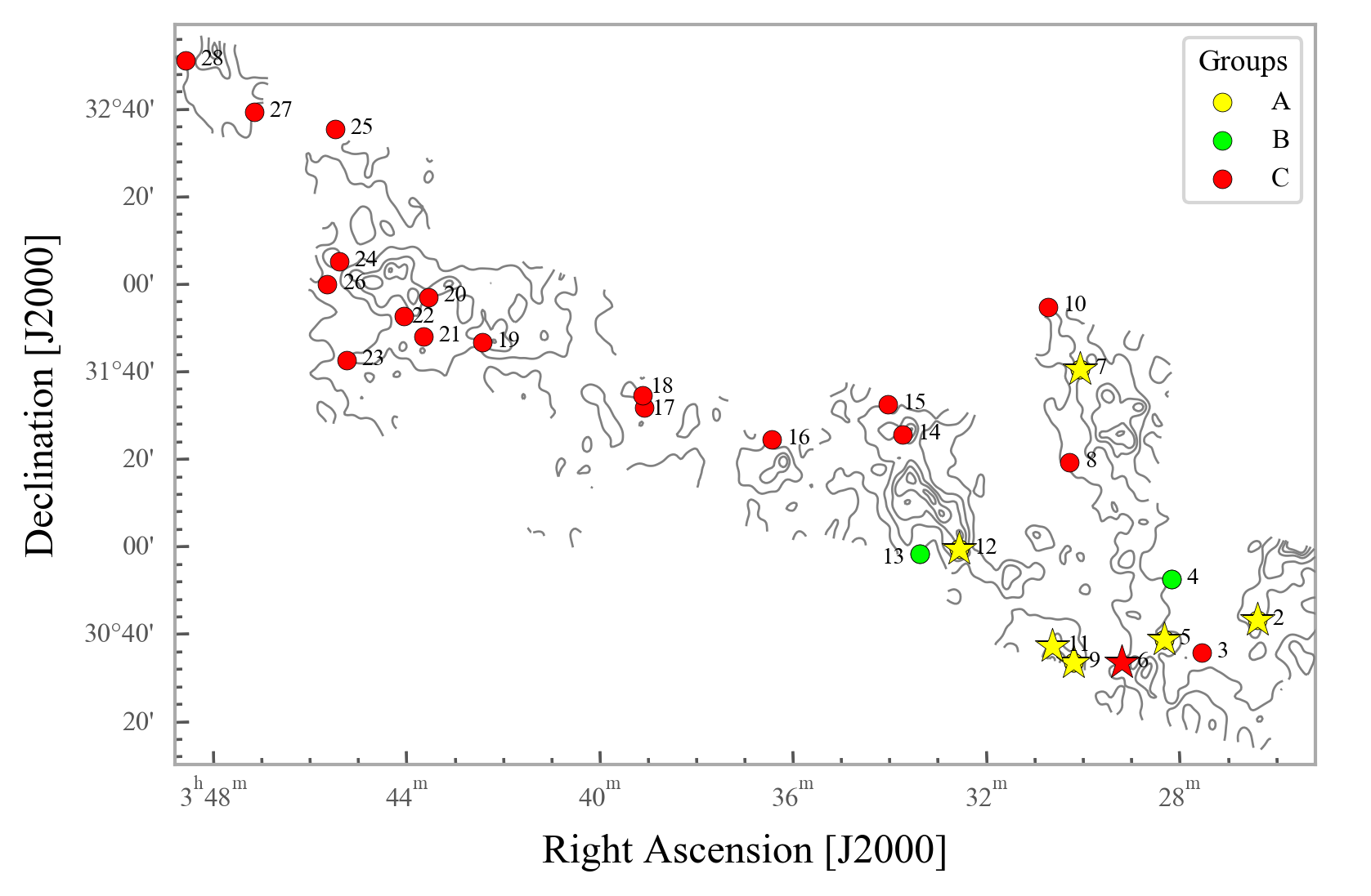
Figure 1: Perseus target positions labeled by alias and overlaid on extinction contours (Evans et al., 2009). The contours represent $A_{\rm V}$ extinction levels of 3, 6, 12, 18, and 24 mag. The target colors refer to the groupings determined in §5.1. Star symbols represent lines of sight with a 3.0 $\mu$m ice band optical depth ($\tau_{\rm 3.0}$) larger than 0.5 within the uncertainties.

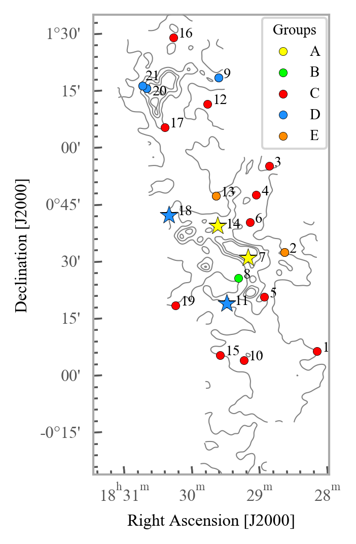
Figure 2: Serpens target positions overlaid on extinction contours (Evans et al., 2009). The contours represent $A_{\rm V}$ extinction levels of 3, 6, 12, 18, and 24 mag. The target colors refer to the groupings determined in §5.1. Star symbols represent lines of sight with an ice band optical depth $\tau_{\rm 3.0}>0.5$ within the uncertainties.

2 Source Selection

Background stars were selected from the Perseus and Serpens molecular clouds which were mapped with Spitzer/IRAC and MIPS by the c2d Legacy team (Evans et al., 2003, 2009). The maps are complete down to $A_{\rm V}$ = 6 and $A_{\rm V}$ = 2 for Serpens and Perseus, respectively (Evans et al., 2003). The selected sources have an overall spectral energy distribution (SED; 2MASS 1.2–2.2 $\mu$m, IRAC 3–8 $\mu$m, MIPS 24 $\mu$m) of a reddened Rayleigh–Jeans curve. They fall in the “star” category in the c2d catalogs and have MIPS 24 $\mu$m to IRAC 8 $\mu$m flux ratios greater than 4. In addition, fluxes are high enough ($>$10 mJy at 8.0 $\mu$m) to obtain Spitzer/IRS spectra of high quality (S/N $>$ 50) within $\sim$20 minutes of observing time per module. This resulted in a list of roughly 100 stars behind Perseus and 400 stars behind Serpens. The list was reduced by selecting $\sim$10 sources in each interval of $A_{\rm V}$ of 2–5, 5–10, and $>$10 mag for Perseus, and 5–10, 10–15, and $>$15 mag for Serpens (taking $A_{\rm V}$ from the c2d catalogs) and making sure that the physical extent of the clouds are covered. For Serpens, there are more background stars to choose from and the overall extinction is higher, reflecting its lower Galactic latitude.

The final target list contains nearly all high $A_{\rm V}$ lines of sight. At low extinctions, many more sources were available and the brightest were selected. The observed samples of 28 targets toward Perseus, and 21 toward Serpens are listed in Tables 1 and 2. The analysis shows that the SEDs of 2 Serpens sources cannot be fitted with stellar models (§5), because they likely have dust shells (silicate band emission). All other targets were found to be usable (hyper)giants or in a few cases main sequence stars. One Perseus target (Per-16) was found to be a foreground, rather than a background star. Reiners & Zechmeister (2020) measure a distance of 13.7 pc to Per-16, which is the closest target in our sample size by far. Indeed, we find no evidence for dust or ice extinction in this line of sight (§5.1).

Figures 1 and 2 plot the location of the observed background stars on extinction map contours derived from 2MASS and Spitzer photometry (Evans et al., 2009).

=5in Alias Name of Star Region Date AOR key Modules Per- 2MASS Ground-based Spitzer/IRS 1 03245605+3026005 LDN 1455 IRS 1 2008-09-27 23083008 SL, LL2 2 03261355+3029223 IRAS 03222+3034 2008-09-30 23085824 SL, LL2 3 03272467+3022547 2008-09-27 23083008 SL, LL2 4 03275729+3040138 LDN 1455 IRS 1 2008-09-30 23082752 SL, LL2 2010-02-05 5 03281034+3026343 LDN 1455 IRS 1 2008-09-29^∗ 23086336 SL, LL2 6 03290508+3022080 LDN 1455 IRS 1 2008-09-30 23087616 SL, LL2 7 03293654+3129465 NGC 1333 2008-09-25^∗ 23088128 SL, LL2 8 03295603+3108454 NGC 1333 2008-09-30 23082752 SL, LL2 9 03300474+3023032 IRAS 03271+3013 2008-09-30 23086592 SL 10 03301239+3144408 NGC 1333 2008-09-28^∗ 23086848 SL 11 03303022+3027087 IRAS 03271+3013 2008-09-25^∗ 23087616 SL, LL2 12 03322030+3050485 IRAS 03292+3039 2008-09-25^∗ 23088384 SL, LL2 13 03331023+3050177 IRAS 03292+3039 2008-09-26 23083776 SL, LL2 14 03332416+3117470 2008-09-29^∗ 23087360 SL, LL2 15 03334078+3125007 2008-09-27 23083776 SL, LL2 2010-02-05 16 03360868+3118398 2008-09-25^∗ 23084800 SL, LL2 17 03384753+3127345 2008-09-26^∗ 23084032 SL, LL 18 03384901+3130173 2008-07-08^∗ 23085312 SL, LL 19 03420993+3144139 2008-09-30 23086080 SL 20 03431627+3155097 IC 348 2010-02-05^∗ 23087872 SL, LL2 21 03432386+3146110 IC 348 2008-09-26^∗ 23085568 SL, LL2 22 03434808+3151030 IC 348 2008-09-28^∗ 23084544 SL, LL2 2008-09-29^∗ 23 03450207+3141196 IC 348 2008-09-27 23084544 SL, LL2 2010-02-05 24 03450796+3204018 IC 348 2008-09-30 23084288 SL, LL2 25 03450839+3234202 2008-09-27 23083264 SL, LL2 2010-02-04 26 03452349+3158573 IC 348 2010-02-04 23083520 SL, LL2 2010-02-05 27 03465115+3238494 2008-09-26 23083264 SL, LL2 2010-02-04 28 03481723+3250595 2008-09-26^∗ 23085568 SL, LL2

Table 1: Perseus Target Observations

Table 2: Serpens Target Observations

Alias	Name of Star	Region	Date	Instrument	AOR key	Modules
Ser-	2MASS		Ground-based		Spitzer/IRS
1	18275901+0002337		2009-10-11	NIRSPEC	23073536	SL, LL2
2	18282010+0029141	Ser/G3-G6	2009-10-11	NIRSPEC	23073792	SL, LL2
3	18282631+0052133		2009-10-11	NIRSPEC	23072768	SL, LL
4	18284038+0044503	Ser/G3-G6	2009-10-11	NIRSPEC	23074816	SL, LL2
5	18284139+0017460	[EGE2007] Bolo 7	2008-07-09	SpeX	23074048	SL, LL2
6	18284797+0037431	Ser/G3-G6	2009-10-11	NIRSPEC	23074304	SL, LL2
7	18285266+0028242	Ser/G3-G6	2007-07-05	NIRSPEC	13460224	SL, LL2
			2021-07-27	SpeX
8	18290316+0023090	[EGE2007] Bolo 7	2009-10-11	NIRSPEC	23076352	SL, LL2
9	18290436+0116207	Core	2009-10-11	NIRSPEC	23074304	SL, LL2
10	18290479-0001301		2008-07-09	SpeX	13210112	SL, LL
11	18291546+0016422	[EGE2007] Bolo 7	2008-07-09	SpeX	23075328	SL, LL
12	18291600+0109382	Core	2008-07-09	SpeX	23073024	SL, LL
13	18291619+0045143	Ser/G3-G6	2009-10-11	NIRSPEC	23073024	SL, LL
14	18291699+0037191		2009-10-11	NIRSPEC	23076096	SL, LL2
15	18292528+0003141		2009-10-11	NIRSPEC	23072768	SL, LL
16	18294108+0127449	Core	2009-10-11	NIRSPEC	23073536	SL, LL2
17	18295604+0104146	Core	2008-07-08	SpeX	23075328	SL, LL
18	18295940+0041007		2008-07-08	SpeX	23075584	SL, LL2
			2008-07-09
19	18300085+0017069		2009-10-11	NIRSPEC	23072768	SL, LL
20	18300896+0114441	Core	2009-10-11	NIRSPEC	23074816	SL, LL2
21	18301220+0115341	Core	2008-07-08	SpeX	23075584	SL, LL2

3 Observations

Spitzer/IRS spectra of background stars toward the Perseus and Serpens clouds were obtained as part of a dedicated Open Time program (PID 40580). Tables 1 and 2 list all sources with their astronomical observation request (AOR) keys and the IRS modules in which they were observed. The SL module, covering the 5–14 $\mu$m range, includes several ice absorption bands, as well as the 9.7 $\mu$m band of silicates, and has the highest signal-to-noise values (S/N$>$50). The LL2 module (14–21 $\mu$m) was included in order to trace the 15 $\mu$m band of solid $\rm{CO_{2}}$ and for a better overall continuum determination, although at a lower S/N of $>$30. At longer wavelengths, the background stars are weaker, and the LL1 module ($\sim$20–35 $\mu$m) was used for only $\sim$30% of the sources. The spectra were extracted and calibrated from the two-dimensional Basic Calibrated Data produced by the standard Spitzer pipeline (version S16.1.0), using the same method and routines discussed in Boogert et al. (2011). Uncertainties (1$\sigma$) for each spectral point were calculated using the “func” frames provided by the Spitzer pipeline.

The Spitzer spectra of Perseus and a subset for Serpens were complemented by ground-based NASA IRTF/SpeX (Rayner et al., 2003) K and L-band spectra. For the remaining Serpens targets, L-band spectra were obtained with the NIRSPEC spectrometer (McLean et al., 1998) on Keck II. The SpeX spectra were obtained in the LongXD1.9 or LongXD2.1 modes, offering wavelength ranges of 1.95-4.2 or 2.15-5.0 $\mu$m, respectively. The M-band portions of these spectra are only presented if they are of sufficiently high quality. The SpeX observations were done under observing programs 2008A079, 2008B074, and 2010A107 spread out over the nights listed in Tables 1 and 2. One target, Ser-7, was observed under program 2021A092 in the LXD_short mode (1.67-4.2 $\mu$m). For all SpeX observations, a slit width of 0.3” was used, yielding a resolving power of R =$\lambda/\Delta\lambda$ = 2500. The spectra were flat fielded, wavelength-calibrated, and extracted using the Spextool package (Cushing et al., 2004). The telluric absorption lines were divided out and the spectra were flux calibrated using the Xtellcor program (Vacca et al., 2003). Standard stars of spectral type A0V were used for this purpose.

The Keck/NIRSPEC spectra of the Serpens targets were observed in the long-slit mode with the 0.57” wide slit, resulting in a resolving power of R = 1,500. Two grating settings were observed, providing a full L-band coverage (2.83-4.2 $\mu$m). The data were reduced from the raw frames in a way standard for ground-based long-slit spectra with the same IDL routines described in Boogert et al. (2008). Sky emission lines were used for the wavelength calibration and bright, nearby main sequence stars were used as telluric and photometric standards. For the division over the standard star, the S/N was optimized by carefully matching the wavelength scale to that of the science targets.

In the end, all SpeX, NIRSPEC, and Spitzer spectra were combined with 2MASS $J$, $H$, and $K_{s}$ broadband photometry (Skrutskie et al., 2006), 3.55, 4.49, 5.73, and 7.87 $\mu$m photometry from c2d Spitzer/IRAC, 24 $\mu$m photometry from Spitzer/MIPS (Evans et al., 2003), and WISE photometry (Wright et al., 2010). The 1-5 $\mu$m spectra were matched to the photometry by convolving them with the $K_{s}$-band filter profile and then multiplying them along the flux scale. Similarly, the Spitzer/IRS spectra were matched to the IRAC 7.87 $\mu$m photometric flux. The same photometry was used in the continuum determination discussed in §4. Catalog flags were taken into account, such that the photometry of sources listed as being confused within a 2” radius or being located within 2” of a mosaic edge were treated as upper limits. The c2d catalogs do not include flags for saturation. Therefore, photometry exceeding the IRAC saturation limit (at the appropriate integration times) was flagged as a lower limit. In those cases, the nearby WISE photometric points were used instead. Finally, as the relative photometric calibration is important for this work, the uncertainties in the Spitzer c2d and 2MASS photometry were increased with the zero-point magnitude uncertainties listed in Table 21 of Evans et al. (2009) and further discussed in Section 3.5.3 of that paper.

4 Methods

To determine the interstellar $A_{\rm K}$, $\tau_{3.0}$, and $\tau_{9.7}$ values, contributions from the stellar photosphere to the observed spectra need to be removed. We did so, following the methods described in Boogert et al. (2011, 2013), and Chu et al. (2020). The fits to the observed spectra were significantly more constrained by combining the spectra with broad-band photometric data (§3).

The fitting process was done in two steps. First, all data available in the 1-5 $\mu$m range were fitted using a large (224) database of template spectra (Rayner et al., 2009) to derive accurate spectral types, as well as $A_{\rm K}$ and $\tau_{3.0}$ values. Second, all data in the full 1-20 $\mu$m range were fitted using a small (13) sample of model spectra (Decin et al., 2004; Boogert et al., 2011) to provide $\tau_{9.7}$. Throughout this paper, the $A_{\rm K}$ and $\tau_{3.0}$ values derived from the 1-5 $\mu$m template fitting process were reported, as they are most accurate considering the much larger database of template spectra available.

All fit parameters are determined simultaneously, and any dependencies are taken into account in the uncertainty estimates. For the 1-5 $\mu$m template fits, this is described in detail in Chu et al. (2020). In short, the key fit parameters are:

1. Spectral Type. The CO overtone lines between 2.25-2.60 $\mu$m provide a sensitive tracer of spectral type. The near-infrared JHK photometry and absorption features in the 3.8-4.1 $\mu$m spectral range also prove to be important for this. The JHK photometry depends on the extinction as well, which is discussed in point 2 below.

2. Continuum Extinction ($A_{\rm K}$). We adopt the commonly used extinction curve from Indebetouw et al. (2005). Due to the steepness of the extinction curve in the 1.0-2.5 $\mu$m region, $A_{\rm K}$ and its uncertainty are primarily determined by the JHK photometry and the shape of the un-reddened spectral template spectrum. The dependency on flux values at longer wavelengths is weak.

3. $\rm{H_{2}O}$ Absorption Feature ($\tau_{3.0}$). $\rm{H_{2}O}$ ice has a prominent broad feature at 3.0 $\mu$m. $\tau_{3.0}$ and its uncertainty are determined by the flux values and the observational noise in the 2.9-3.2 $\mu$m range, including dependencies on the accuracy of the baseline surrounding the ice feature. For the fitting, an $\rm{H_{2}O}$ ice absorption spectrum for spherical, pure ice grains using optical constants of amorphous ice at a temperature of 10 K (Hudgins et al., 1993) is assumed. A grain size of 0.4 $\mu$m is chosen. This particular ice temperature and grain size have no significance other than that they match the shape of the 3.0 $\mu$m band well, providing a tool to derive $\tau_{3.0}$.

Besides the reduced $\chi^{2}$ values derived for the individual wavelength regions discussed above, a total reduced $\chi^{2}$ ($\chi_{\nu}^{2}$) is calculated across the wavelength range of 1-4 $\mu$m, using the IRTF template database. Where this $\chi_{\nu}^{2}$ is lowest, the model template is chosen as the best fit to the star. The final errors for $A_{\rm K}$ and $\tau_{3.0}$ are increased by including all of the model templates that have $\chi_{\nu}^{2}$ (1-4 $\mu$m) within a factor of 2 of the best template. This represents a confidence level of at least 3$\sigma$. In some cases, the uncertainties on $A_{\rm K}$ and $\tau_{3.0}$ are much smaller than expected from the $\chi_{\nu}^{2}$ across the full 1-4 $\mu$m wavelength range, because $A_{\rm K}$ and $\tau_{3.0}$ depend strongly on only a sub-set of this wavelength range.

For the full 1-21 $\mu$m fits, using a much smaller set of stellar models, $\tau_{3.0}$ is kept fixed. The strength and shape of the longer wavelength $\rm{H_{2}O}$ ice bands is set by assuming the $\rm{H_{2}O}$ ice model discussed above. The 9.7 $\mu$m silicate band is fitted for grains small compared to the wavelength, having a pyroxene to olivine optical depth ratio of 0.62 at the 9.7 $\mu$m peak (Boogert et al., 2011). A key factor in the fitting process is the photospheric SiO band at $\sim$8 $\mu$m, as it overlaps with the 9.7 $\mu$m band of silicate dust. For some targets, the model spectral types were optimized to fit that photospheric band best. Also, in some cases the models were normalized to the data at a wavelength of 8.0 $\mu$m, instead of the default of 5.5 $\mu$m. This provides a better local baseline for the silicate feature, while reducing the fit quality at other wavelengths. Accurate $\tau_{9.7}$ values are more important for this work than a good fit over the larger wavelength range.

5 Results

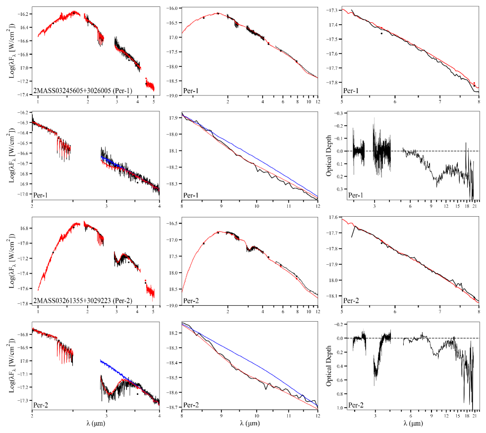
Figure 15: The model fits and optical depth plots of the 28 Perseus and 21 Serpens targets. Each target has a 2x6 format of its plots: short wavelength IRTF model (top left), full wavelength IRTF and Spitzer model (top middle), 5-8 $\mu$m (top right), 2-4 $\mu$m (bottom left), 8-12 $\mu$m (bottom middle), and optical depth (bottom right). Black indicates the observed data, and red the model data. The 2-4 $\mu$m plot indicates any presence of the 3 $\mu$m OH stretch mode, which is made more prominent by the blue model flux which has the $\rm{H_{2}O}$ ice contribution omitted; the models do not include parameters to fit the wings around 3.4 $\mu$m. The 8-12 $\mu$m plot indicates any presence of the 9.7 $\mu$m silicates, which is made more prominent by the blue model flux which has the silicates contribution omitted. The 5-8 $\mu$m plot indicates any presence of the 6 $\mu$m OH stretch mode and the 6.85 $\mu$m absorption feature due to, tentatively, NH${}_{4}^{+}$.

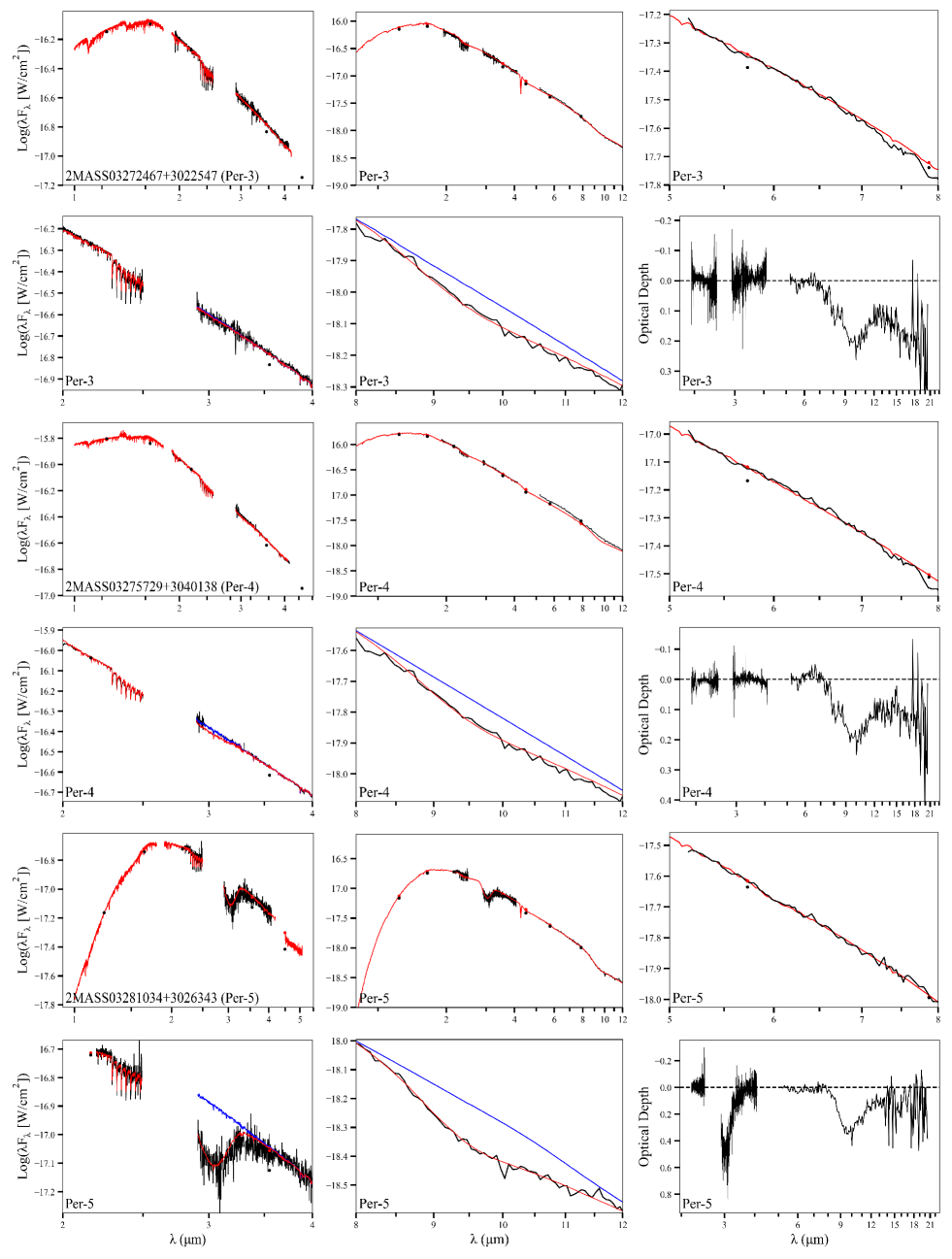
Figure 15: (Continuation)

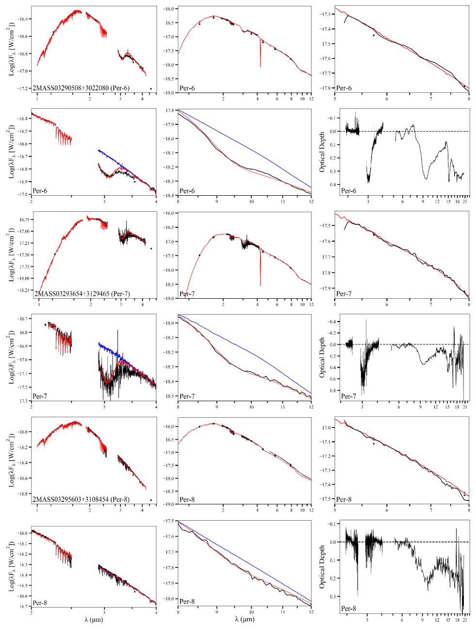
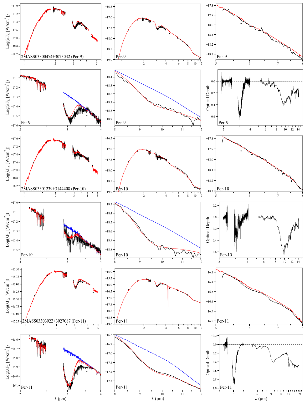
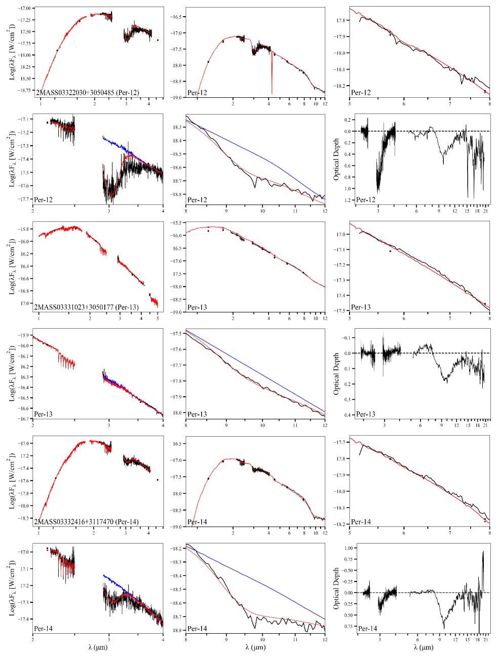
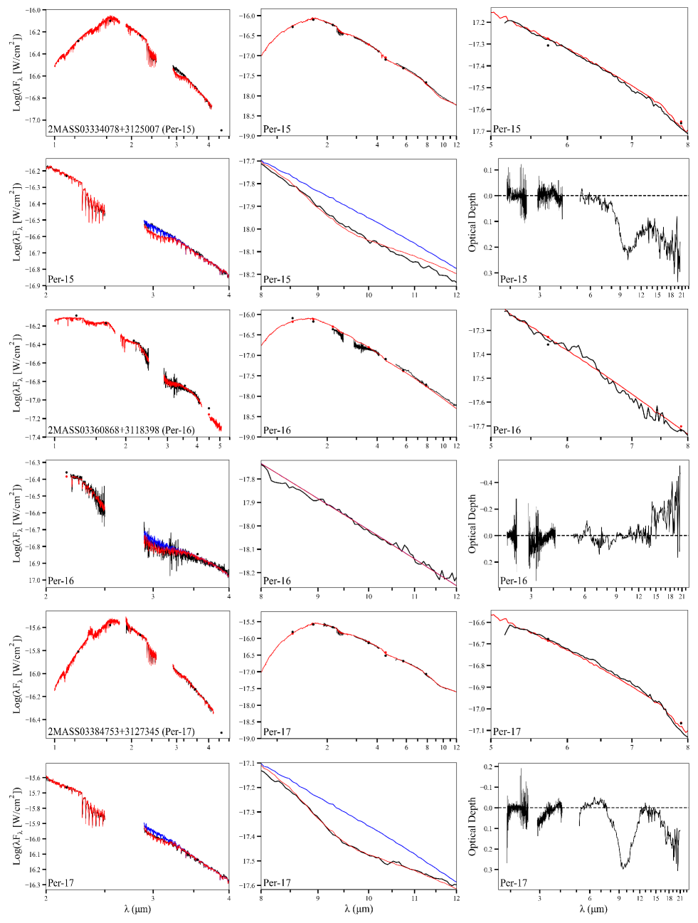
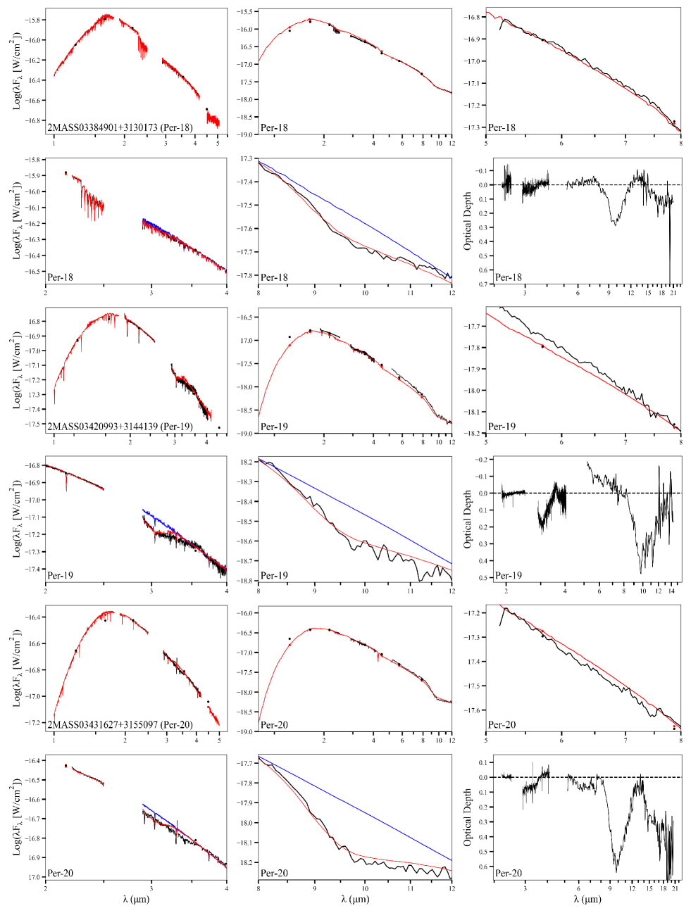
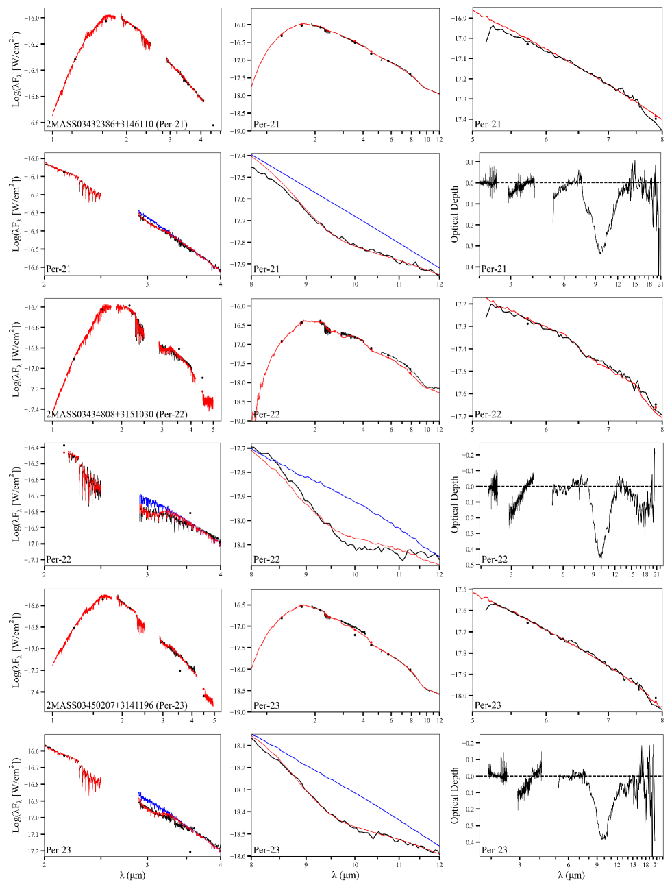
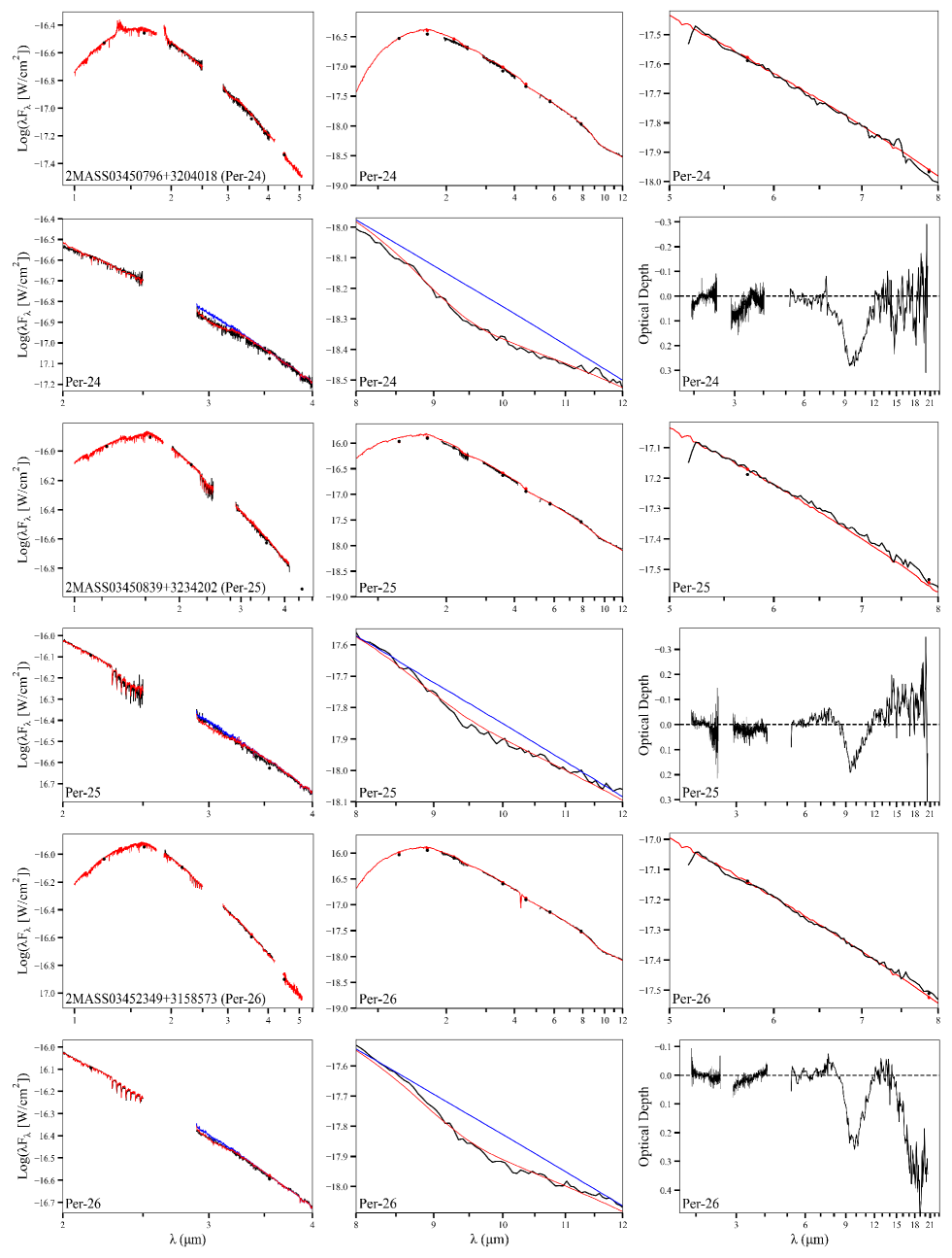
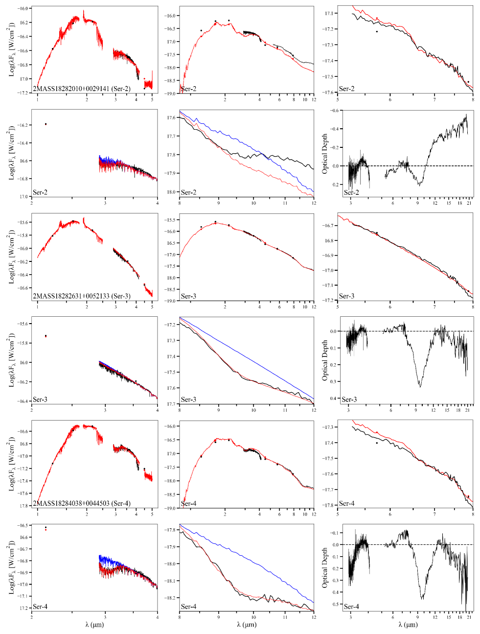
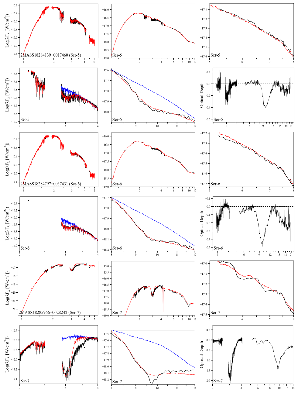
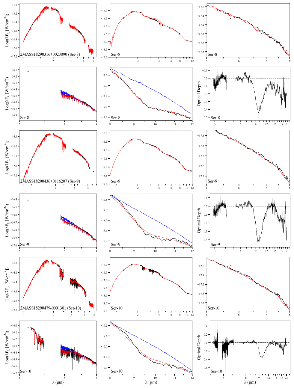
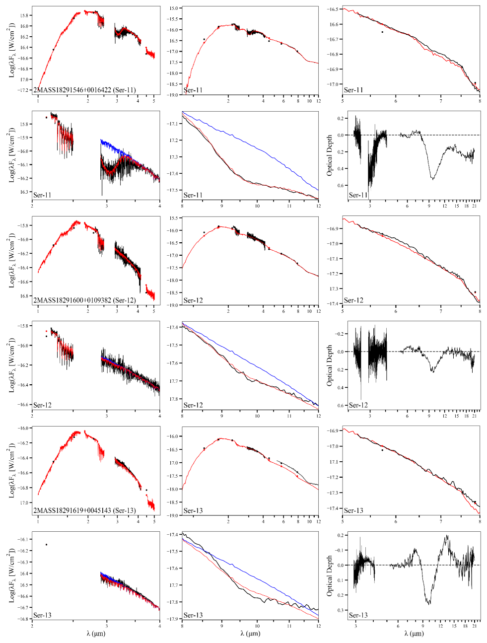
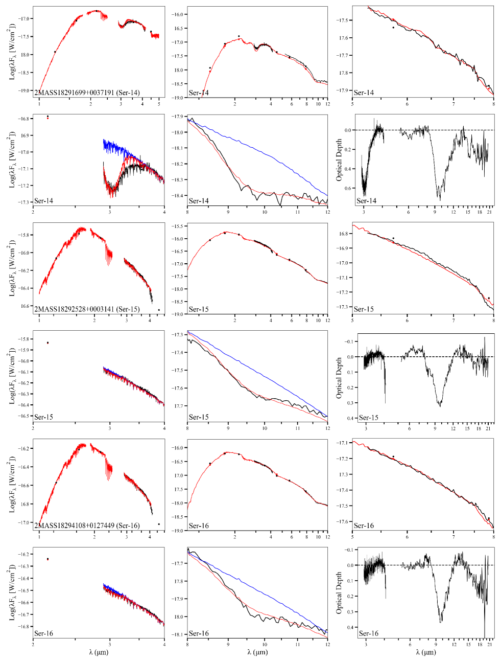
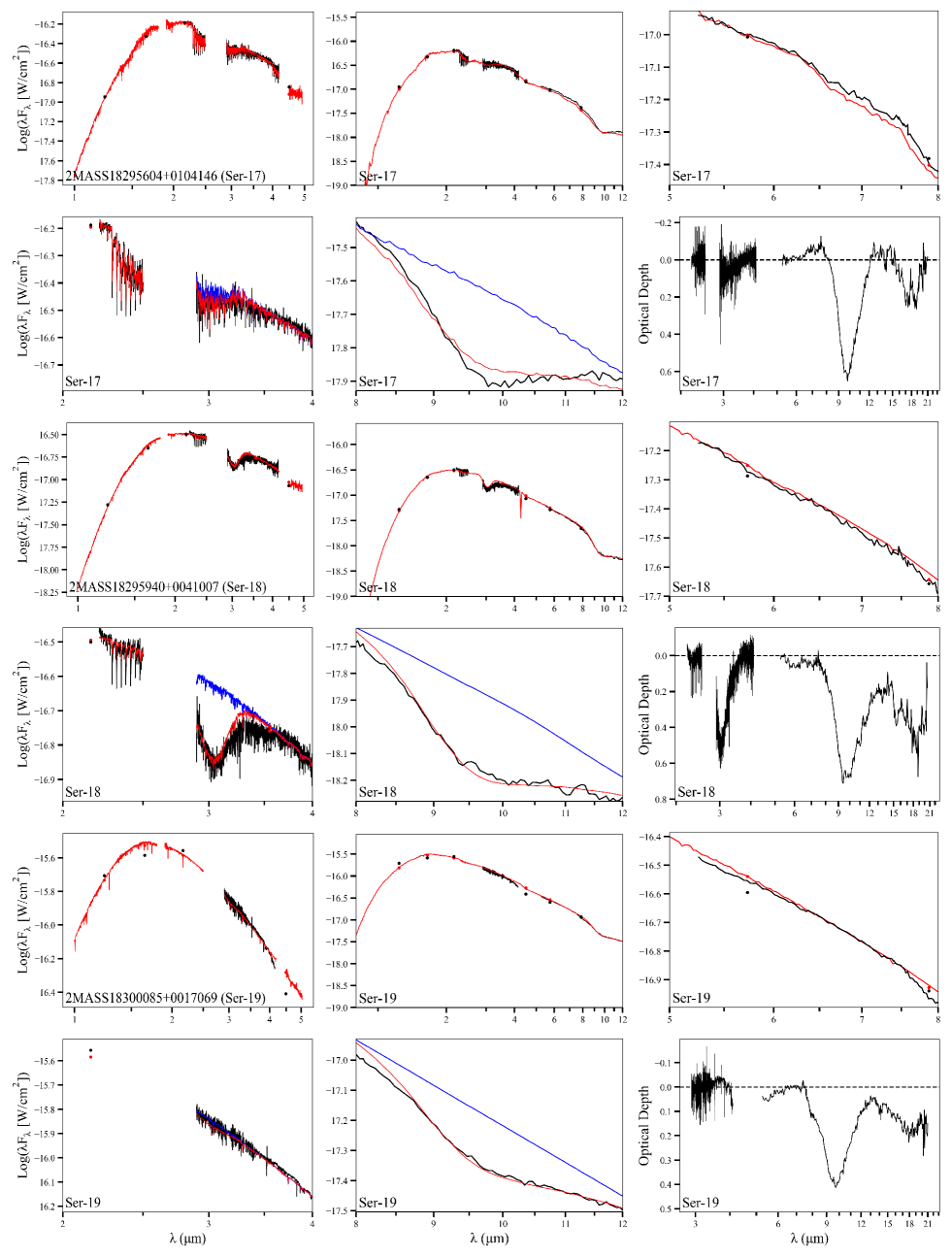
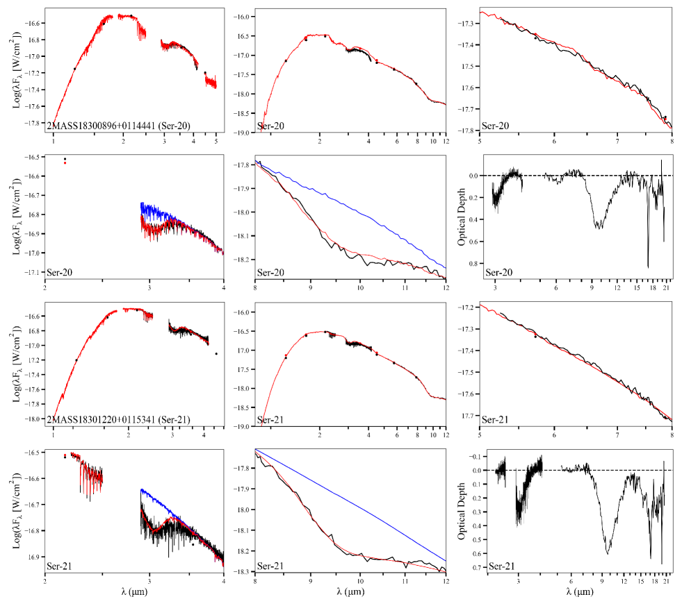
Figure 15: (Continuation)

Using the models described in §4, the values for $A_{\rm K}$, $\tau_{3.0}$, and $\tau_{9.7}$ are derived. The best fitting models are shown in Fig. 15 and the derived values in Tables 3 and 4.

Table 3: Perseus Target Results

Alias	IRTF Template	Model	$A_{\rm K}$	$\tau_{3.0}$	$\tau_{9.7}$	$\chi_{\nu}^{2}$	N($\rm{H_{2}O_{ice}}$)	Notes
(Per-)	1-5 $\mu$m	1-30 $\mu$m	mag				$10^{17}\rm{cm}^{-2}$
1	HD16068 (K3.5II)	K4III	0.34 $\pm$ 0.07	0.0 $\pm$ 0.12	0.26 $\pm$ 0.09	2.92	$<$1.94	L-band = 1.15
2	HD170820 (G9II)	K0III	0.92 $\pm$ 0.08	0.49 $\pm$ 0.17	0.23 $\pm$ 0.05	0.76	7.87 $\pm$ 2.73	L-band = 1.15
3	HD44391 (K0I)	K0III	0.30 $\pm$ 0.08	0.01 $\pm$ 0.05	0.24 $\pm$ 0.07	0.57	$<$0.83	…
4	HD222093 (G9III)	G8III	0.22 $\pm$ 0.06	0.0 $\pm$ 0.05	0.22 $\pm$ 0.05	2.02	$<$0.81	L-band = 1.02
5	HD202314 (G6I)	G8III	1.27 $\pm$ 0.09	0.49 $\pm$ 0.06	0.33 $\pm$ 0.05	0.51	7.91 $\pm$ 0.97	L-band = 1.13
6	HD44391 (K0I)	G8III	0.75 $\pm$ 0.07	0.39 $\pm$ 0.08	0.38 $\pm$ 0.05	1.70	6.29 $\pm$ 1.36	L-band = 0.93
7	HD35620 (K3.5III)	K4III	1.63 $\pm$ 0.05	0.55 $\pm$ 0.05	0.35 $\pm$ 0.05	0.24	8.97 $\pm$ 0.82	L-band = 0.97
8	HD44391 (K0I)	K0III	0.43 $\pm$ 0.15	0.01 $\pm$ 0.11	0.26 $\pm$ 0.05	0.5	$<$1.78	L-band = 1.07
9	HD192713 (G3I)	G8III	1.41 $\pm$ 0.05	0.52 $\pm$ 0.05	0.41 $\pm$ 0.05	0.67	8.47 $\pm$ 0.86	L-band = 1.06
10	HD9852 (K0.5III)	K4III	1.32 $\pm$ 0.14	0.24 $\pm$ 0.08	0.57 $\pm$ 0.07	1.11	3.81 $\pm$ 1.27	…
11	HD132935 (K2III)	K5III	1.69 $\pm$ 0.07	0.84 $\pm$ 0.05	0.43 $\pm$ 0.05	1.24	13.66 $\pm$ 0.82	L-band = 1.07
12	HD182694 (G7III)	G8III	1.87 $\pm$ 0.12	0.92 $\pm$ 0.11	0.38 $\pm$ 0.07	1.11	14.9 $\pm$ 1.79	L-band = 0.92
13	HD9852 (K0.5III)	G8III	0.21 $\pm$ 0.17	0.0 $\pm$ 0.05	0.19 $\pm$ 0.05	1.08	$<$0.81	…
14	HD91810 (K1III)	K3III	1.43 $\pm$ 0.05	0.29 $\pm$ 0.11	0.57 $\pm$ 0.09	0.81	4.76 $\pm$ 1.80	…
15	HD120477 (K5.5III)	K7III	0.42 $\pm$ 0.11	0.0 $\pm$ 0.10	0.24 $\pm$ 0.08	3.24	$<$1.62	L-band = 1.03
16	Gl581 (M2.5V)	G8III	0.0 $\pm$ 0.05	0.09 $\pm$ 0.05	0.0 $\pm$ 0.05	3.65	1.41 $\pm$ 0.78	L-band = 0.93
17	HD35620 (K3.5III)	K7III	0.67 $\pm$ 0.12	0.08 $\pm$ 0.05	0.29 $\pm$ 0.07	0.59	1.32 $\pm$ 0.82	L-band = 0.95
18	HD213893 (M0III)	K4III	0.58 $\pm$ 0.09	0.04 $\pm$ 0.05	0.24 $\pm$ 0.06	0.71	$<$0.84	L-band = 0.98
19	HD108519 (F0V)	G8III	0.98 $\pm$ 0.05	0.18 $\pm$ 0.06	0.35 $\pm$ 0.07	1.17	2.91 $\pm$ 0.97	local 9.7 $\mu$m baseline
20	HD160365 (F6III)	G8III	1.23 $\pm$ 0.13	0.1 $\pm$ 0.06	0.54 $\pm$ 0.06	4.09	1.63 $\pm$ 0.98	L-band = 0.95
21	HD222093 (G9III)	G8III	0.95 $\pm$ 0.08	0.06 $\pm$ 0.05	0.34 $\pm$ 0.05	0.68	0.97 $\pm$ 0.81	L-band = 0.98
22	HD4408 (M4III)	M6III	0.95 $\pm$ 0.06	0.19 $\pm$ 0.05	0.33 $\pm$ 0.08	2.99	3.01 $\pm$ 0.79	L-band=0.83, local 9.7 $\mu$m baseline
23	HD132935 (K2III)	K4III	0.71 $\pm$ 0.1	0.13 $\pm$ 0.08	0.37 $\pm$ 0.05	0.80	2.09 $\pm$ 1.29	L-band = 0.90
24	HD10697 (G3V)	G8III	0.61 $\pm$ 0.11	0.09 $\pm$ 0.09	0.27 $\pm$ 0.05	1.18	1.49 $\pm$ 1.49	L-band = 0.95
25	HD100006 (K0III)	K0III	0.35 $\pm$ 0.09	0.0 $\pm$ 0.06	0.12 $\pm$ 0.05	1.77	$<$0.97	…
26	HD16139 (G8.5III)	G8III	0.49 $\pm$ 0.09	0.04 $\pm$ 0.05	0.20 $\pm$ 0.05	0.89	$<$0.83	…
27	HD132935 (K2III)	K3III	0.37 $\pm$ 0.05	0.05 $\pm$ 0.05	0.22 $\pm$ 0.05	0.49	0.83 $\pm$ 0.83	…
28	HD35620 (K3.5III)	K4III	0.76 $\pm$ 0.12	0.23 $\pm$ 0.11	0.26 $\pm$ 0.05	0.51	3.72 $\pm$ 1.78	L-band = 0.95

Note. — Perseus targets observed by alias along with the fitted IRTF templates, full spectra templates assuming spectral types, extinctions, water ice optical depths, silicate optical depths, $\chi_{\nu}^{2}$ values for the IRTF template database fits, water ice column densities, and extra notes.

Table 4: Serpens Target Results

Alias	IRTF Template	Model	$A_{\rm K}$	$\tau_{3.0}$	$\tau_{9.7}$	$\chi_{\nu}^{2}$	N($\rm{H_{2}O_{ice}}$)	Notes
(Ser-)	1-5 $\mu$m	1-30 $\mu$m	mag				$10^{17}\rm{cm}^{-2}$
1	HD204724 (M1III)	M1III	0.73 $\pm$ 0.23	0.10 $\pm$ 0.10	0.24 $\pm$ 0.05	0.86	1.64 $\pm$ 1.64	…
2	HD196610 (M6III)	M7III	0.87 $\pm$ 0.16	0.10 $\pm$ 0.18	—	1.25	$<$2.93	…
3	HD179870 (K0II)	K3III	0.75 $\pm$ 0.19	0.03 $\pm$ 0.06	0.31 $\pm$ 0.05	1.91	$<$0.97	L-band = 0.95
4	HD28487 (M3.5III)	M3III	1.12 $\pm$ 0.17	0.24 $\pm$ 0.12	0.38 $\pm$ 0.08	1.18	3.81 $\pm$ 1.91	…
5	HD64332 (S4.5)	M1III	1.09 $\pm$ 0.07	0.22 $\pm$ 0.08	0.36 $\pm$ 0.05	0.24	3.62 $\pm$ 1.32	L-band = 1.10
6	HD4408 (M4III)	M1III	1.01 $\pm$ 0.05	0.21 $\pm$ 0.09	0.44 $\pm$ 0.07	0.64	3.32 $\pm$ 1.42	local 9.7 $\mu$m baseline
7	HD18191 (M6III)	M6III	4.75 $\pm$ 0.44	1.63 $\pm$ 0.06	1.18 $\pm$ 0.06	0.87	26.33 $\pm$ 0.97	L-band = 1.10, local 9.7 $\mu$m baseline
8	HD4408 (M4III)	M6III	0.73 $\pm$ 0.05	0.09 $\pm$ 0.05	0.42 $\pm$ 0.05	0.64	1.52 $\pm$ 0.85	…
9	HD201065 (K4I)	M0III	0.92 $\pm$ 0.40	0.08 $\pm$ 0.07	0.37 $\pm$ 0.05	1.01	1.38 $\pm$ 1.20	…
10	HD39045 (M3III)	M1III	0.73 $\pm$ 0.08	0.13 $\pm$ 0.13	0.31 $\pm$ 0.05	0.26	2.18 $\pm$ 2.18	L-band = 0.95
11	HD204724 (M1III)	M6III	1.44 $\pm$ 0.12	0.47 $\pm$ 0.13	0.54 $\pm$ 0.05	0.48	7.66 $\pm$ 2.12	…
12	HD204724 (M1III)	M0III	0.71 $\pm$ 0.13	0.03 $\pm$ 0.11	0.19 $\pm$ 0.06	3.03	$<$1.81	L-band = 1.10
13	HD194193 (K7III)	M1III	0.78 $\pm$ 0.15	0.05 $\pm$ 0.12	—	0.94	$<$2.02	L-band = 1.15
14	HD4408 (M4III)	M6III	2.03 $\pm$ 0.09	0.63 $\pm$ 0.20	0.61 $\pm$ 0.09	0.89	10.16 $\pm$ 3.22	local 9.7 $\mu$m baseline
15	HD201065 (K4I)	K7III	0.69 $\pm$ 0.33	0.03 $\pm$ 0.05	0.29 $\pm$ 0.08	0.81	$<$0.82	…
16	HD201065 (K4I)	M1III	0.83 $\pm$ 0.24	0.06 $\pm$ 0.07	0.28 $\pm$ 0.08	1.13	$<$1.15	…
17	HD94705 (M5.5III)	M6III	1.40 $\pm$ 0.05	0.08 $\pm$ 0.18	0.54 $\pm$ 0.13	0.39	$<$2.88	…
18	HD108477 (G4III)	G8III	1.91 $\pm$ 0.20	0.50 $\pm$ 0.05	0.74 $\pm$ 0.06	0.54	8.13 $\pm$ 0.81	L-band = 1.08
19	HD11443 (F6IV)	G8III	0.98 $\pm$ 0.24	0.0 $\pm$ 0.05	0.43 $\pm$ 0.06	3.50	$<$0.81	…
20	HD28487 (M3.5III)	M6III	1.19 $\pm$ 0.15	0.24 $\pm$ 0.12	0.43 $\pm$ 0.05	0.93	3.87 $\pm$ 1.94	…
21	HD44391 (K0I)	G8III	1.61 $\pm$ 0.10	0.29 $\pm$ 0.05	0.57 $\pm$ 0.05	0.48	4.63 $\pm$ 0.80	L-band = 1.07

Note. — Serpens targets observed by alias along with the fitted IRTF templates, full spectra templates assuming spectral types, extinctions, water ice optical depths, silicate optical depths, the total reduced $\chi_{\nu}^{2}$ values for the IRTF template database fits, water ice column densities, and extra notes.

The fits to the 1-5 $\mu$m wavelength region, using the IRTF template database, are generally good. In a fair number of cases, however, we did notice deficiencies in fitting the continuum region near 4.0 $\mu$m, even though the data at shorter wavelengths were fitted well. This could be due to calibration errors in the slope of the 2-4 $\mu$m SpeX spectra or in the Spitzer or WISE photometry used to calibrate the NIRSPEC spectra (for which no $K-$band portion is available). It could also reflect an uncertainty in the extinction curve or incompleteness of the spectral database. Regardless of the origin, we reduced the effect on the derived $\tau_{3.0}$ by scaling the L-band spectrum to match the best-fitting model. The scaling factors are provided in Tables 3 and 4. In five cases, this correction factor is less than 5%, and in twenty-three cases 5-17%. We are confident in the derived values of $\tau_{3.0}$, as the absorption band can be distinguished by the shape to the $L-$band spectrum, and the adjustments are essentially local baseline corrections.

Of all 49 targets, 7 have deviating slopes in the 8-12 $\mu$m region, even though the IRTF template fits in the 1-5 $\mu$m range are good. This may reflect the small number of 1-20 $\mu$m photospheric models available. In order to improve the fit of the 9.7 $\mu$m silicate feature, a local baseline correction was applied by changing the wavelength range for which the model is normalized to the observations from the default of 5.34-5.50 $\mu$m to 7.3-7.5 $\mu$m. However, for two of these targets (Ser-2 and Ser-13), this approach was insufficient. The deviations from the model are very large, and there is a hint of silicate emission affecting the shape of the 9.7 $\mu$m absorption feature. For these, probably more evolved, mass losing stars, we discarded the derived $\tau_{9.7}$ values. For another 10 targets, while the 8-12 $\mu$m slopes are in good agreement with the spectral types derived from the 1-5 $\mu$m range, the 8 $\mu$m SiO photospheric absorption band suggests later spectral types. Such inconsistency was also noted for several Lupus background stars (Boogert et al., 2013). The affected targets are indicated in Tables 3 and 4, and the effect on the reported $\tau_{9.7}$ values was taken into account.

5.1 $\tau_{9.7}$ and $A_{\rm K}$ Correlation

Analogous to earlier work (Chiar et al., 2007; Boogert et al., 2013), we plot the derived values for $\tau_{9.7}$ against $A_{\rm K}$ (Fig. 3). The rising trend is fitted with:

$$\tau_{9.7}=m\times A_{\rm K}$$ (1)

We find that for Perseus, $m=0.416\pm 0.026$, and for Serpens, $m=0.406\pm 0.041$. A significant amount of scatter is visible in these plots, especially for Perseus. In order to investigate the origin of these variations, we separate the target into different groups. Throughout this work, we will refer to these as Groups A to E.

The targets that fall at least $6\sigma$ below the linear fit are referred to as “Group A.” Those that are at least $6\sigma$ above this relation will be referred to as “Group B.” As can be seen in Fig. 3, Group A targets follow the Lupus IV dense cloud relation ($m=0.26$; Boogert et al., 2013), and Group B targets follow the diffuse ISM relation ($m=0.554$; Whittet, 2003). Based on this, targets that fall within $6\sigma$ of more than one of these three relations are assigned to “Group C,” and targets that exclusively follow the fits over all targets are in “Group D.” Only Serpens exhibits this latter Group. For Perseus, several Group C targets follow the overall fit, but the uncertainties are too large to assign them to Group D. Finally, targets for which no reliable $\tau_{9.7}$ values could be derived, but that do have $A_{\rm K}$ and $\tau_{3.0}$ measurements, are in “Group E.” Also, note that one target (Per-16) has $A_{\rm K}=0.0\pm 0.05$ (Table 3), which is consistent with its distance of 13.7 pc (Reiners & Zechmeister, 2020), indicating this target is actually a Perseus foreground, rather than background, star.

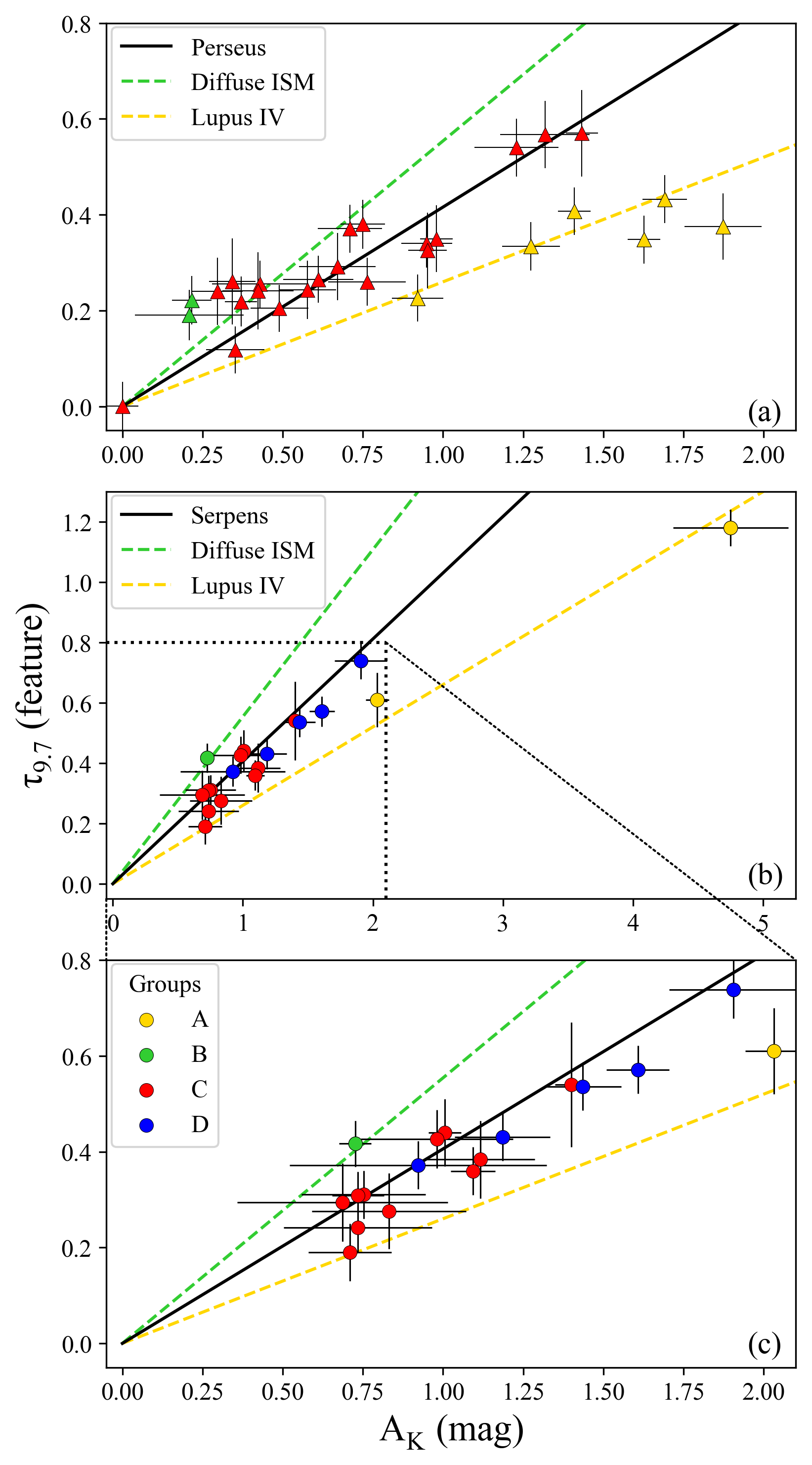
Figure 3: Silicate band optical depth and extinction correlation for Perseus (a) and Serpens (b and c) targets. The error bars are of 3$\sigma$ significance. The solid black line is a least square fit to all targets in the cloud. The dashed yellow line is the Lupus IV correlation from Boogert et al. (2013). The dashed green line is the Diffuse ISM correlation from Whittet (2003). Panel c zooms in on the lower extinction Serpens targets. The colors of the bullets represent the groups defined in §5.1, and are indicated in panel c. They apply to panels a and b as well as to the other Figures in this paper.

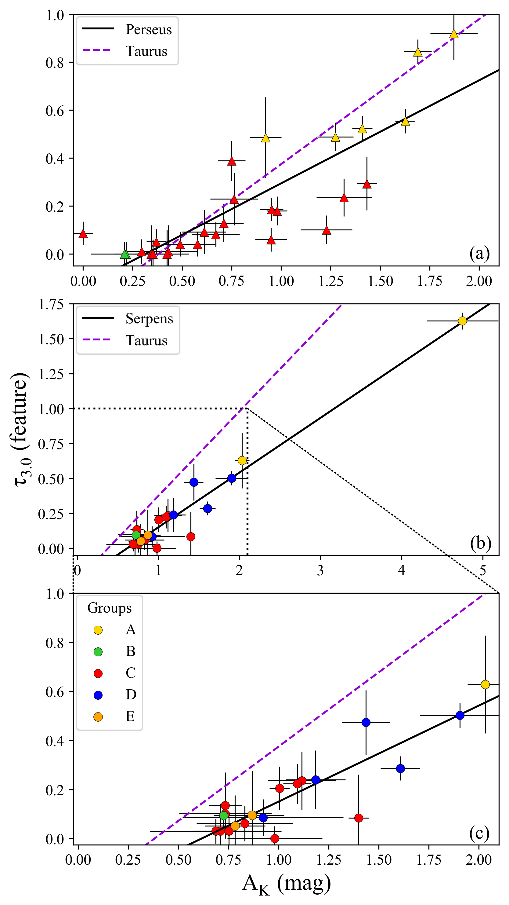
Figure 4: Water ice band optical depth and extinction correlations for Perseus (a) and Serpens (b and c) targets. The error bars are of 3$\sigma$ significance. The solid black line is a least square fit to all targets in the cloud. The dashed purple line is the Taurus molecular cloud correlation from Whittet et al. (2001). The colors of the data points correspond to the groupings defined in §5.1 and Fig. 3. Panel c zooms in on the lower extinction Serpens targets.

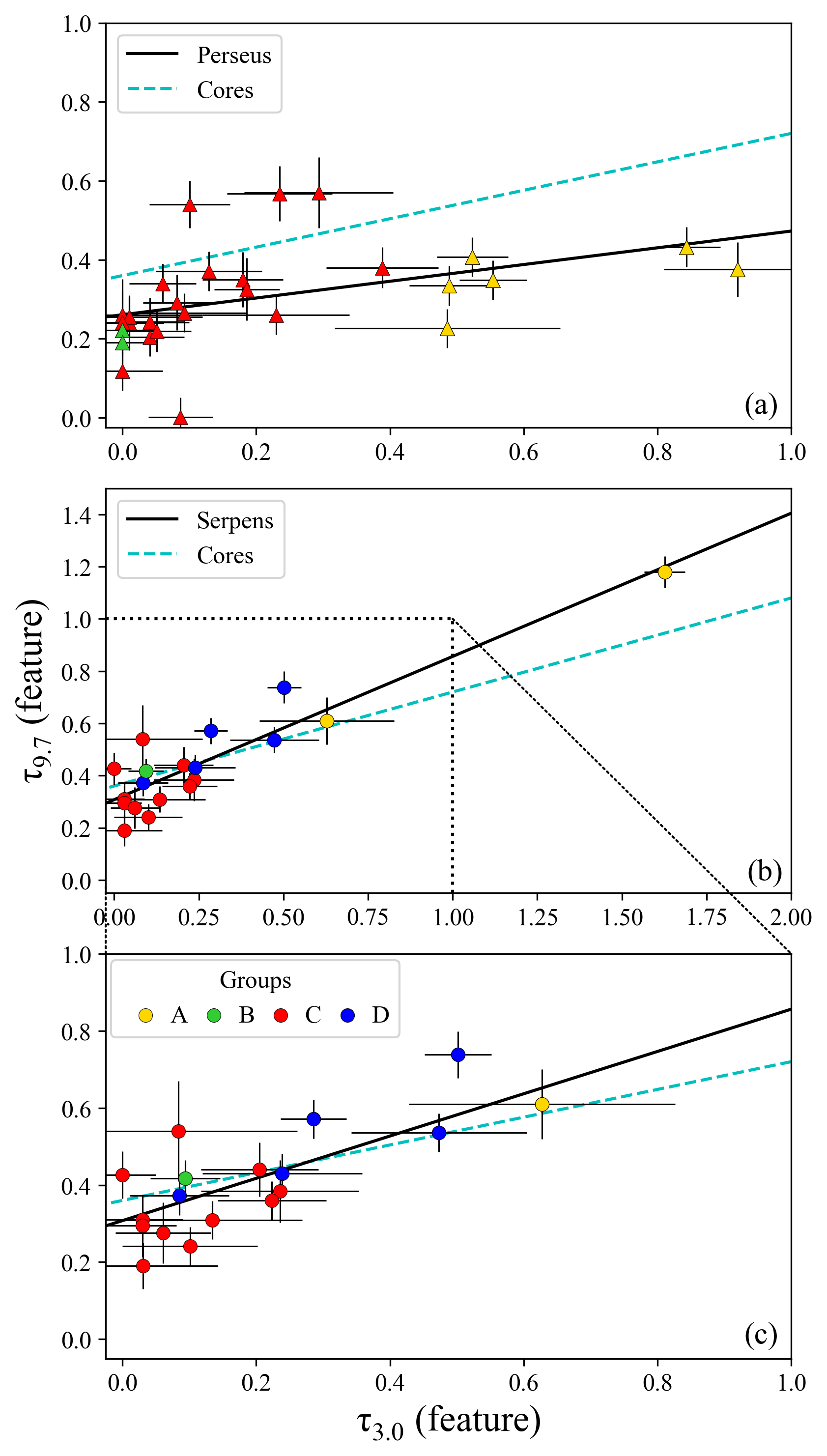
Figure 5: Water ice and silicate band optical depth correlations for Perseus (a) and Serpens (b and c) targets. The error bars are of 3$\sigma$ significance. The solid black line is a least square fit to all targets in the cloud. The dashed blue line is the correlation derived from dense cores in Boogert et al. (2011). The colors of the data points correspond to the groupings defined in §5.1 and Fig. 3. Panel c zooms in on the lower extinction Serpens targets.

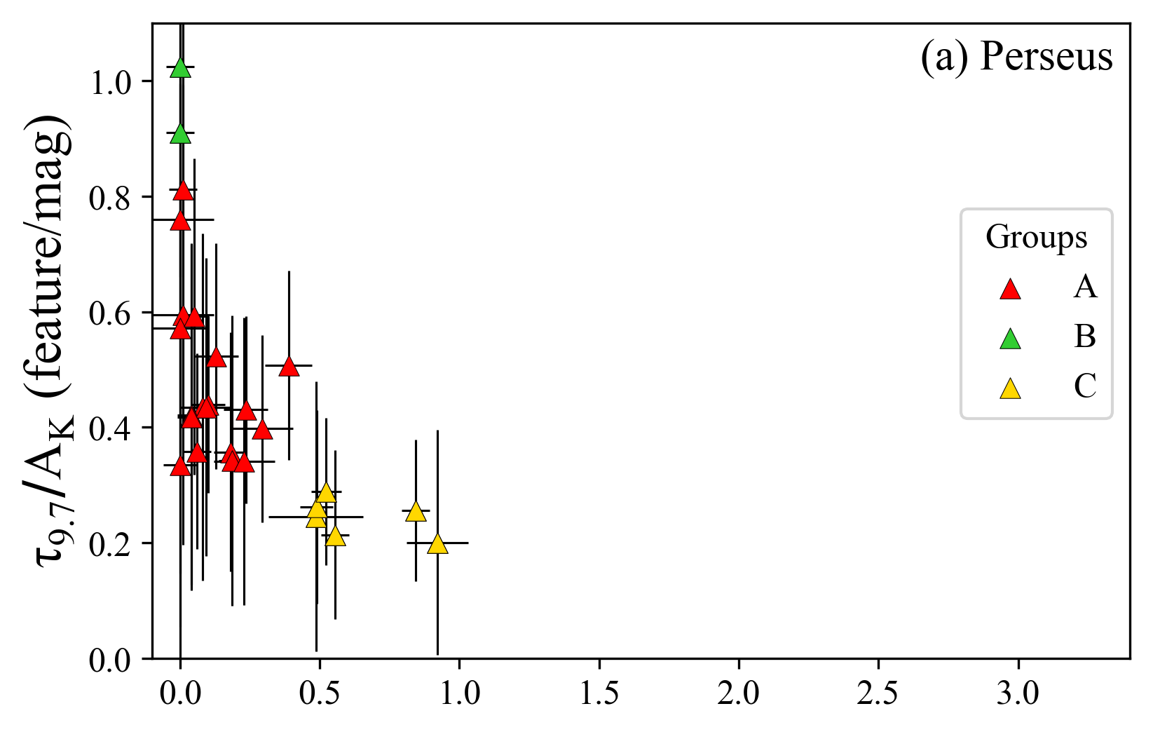
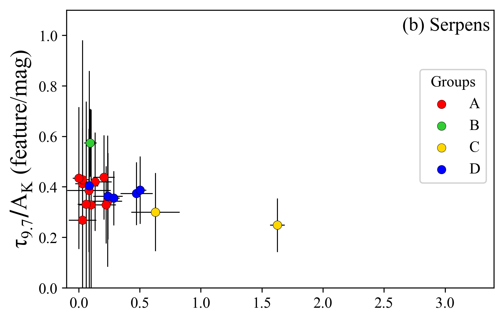
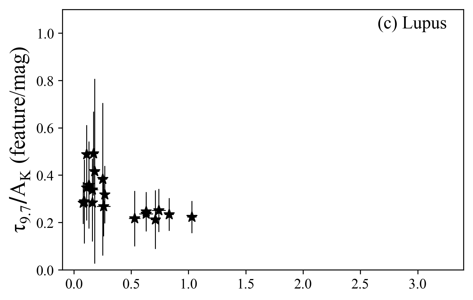
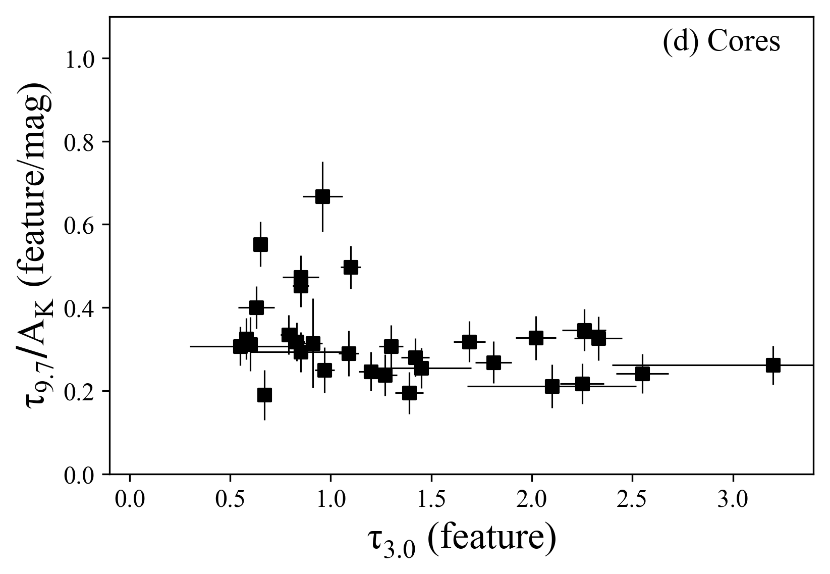
Figure 6: Relation between the $\tau_{9.7}$/$A_{\rm K}$ ratio and $\tau_{3.0}$ for Perseus (a), Serpens (b), and Lupus (c) clouds, as well as isolated dense cores (d). The error bars are of 3$\sigma$ significance. The colors of the data points in panels a and b correspond to the groupings in Fig. 3.

5.2 $\tau_{3.0}$ and $A_{\rm K}$ Correlation

The relation between $\tau_{3.0}$ and $A_{\rm K}$ can be used to determine the ice formation threshold (e.g., Whittet et al., 2001) and to determine the abundance of ices relative to dust. This relation is plotted for Perseus and Serpens in Fig. 4. Generally, $\tau_{3.0}$ increases as a function of $A_{\rm K}$, and the relation does not go through the origin. The data points are therefore fitted with the function:

$$\tau_{3.0}=a\times A_{\rm K}+b$$ (2)

We find that for Perseus, $a=0.430\pm 0.054$ and $b=-0.136\pm 0.052$, and for Serpens, $a=0.391\pm 0.021$ and $b=-0.241\pm 0.032$. The abscissa of this relation gives the ice formation threshold. For Perseus this is $A_{\rm K}=0.315\pm 0.127$, and for Serpens $A_{\rm K}=0.616\pm 0.087$. The Perseus values are comparable to those for Lupus IV: $a=0.44\pm 0.03$ and $b=-0.11\pm 0.03$, and an ice formation threshold of $A_{\rm K}=0.25\pm 0.07$ (Boogert et al., 2013). The Serpens ice formation threshold is almost twice that of the other clouds, which may relate to unrelated foreground extinction at the larger distance of Serpens (§6.3; Zucker et al. 2019).

For Perseus, $\tau_{3.0}$ shows a significant scatter as a function of $A_{\rm K}$ (Fig. 4a). By indicating the different groups identified in the $\tau_{9.7}$ versus $A_{\rm K}$ correlation (§5.1), it is evident that the Group A targets, i.e., those with the most suppressed, “dense core-like” silicate bands, have deeper water ice bands at a given $A_{\rm K}$ than the Group C targets. These Group A targets closely follow the Taurus ice correlation, within $3\sigma$ ($a=0.60\pm 0.02$, $b=-0.23\pm 0.01$; Whittet et al. 2001).

For Serpens (Fig. 4b and c), all targets have $\tau_{3.0}$ values that fall significantly below the Taurus correlation. This is not only reflected in the higher extinction threshold derived above, but also in the shallower slope of the correlation. The latter might indicate lower $\rm{H_{2}O}$ ice abundances in Serpens compared to Taurus. It might also be a reflection of smaller grain sizes in Serpens, enhancing $A_{\rm K}$ relative to $\tau_{3.0}$ (§6.1). Here again, the different groups, distinguished in the $\tau_{9.7}$ versus $A_{\rm K}$ correlation, are indicated. All groups follow the same correlation, but Group A targets are higher on the correlation than Group C and D targets, respectively. It is also worth noting that all targets, with the exception of Ser-19 (Group C), have $\rm{H_{2}O}$ ice detections, including the Group B “diffuse ISM” target Ser-8.

5.3 $\tau_{3.0}$ and $\tau_{9.7}$ Correlation

The relations between $\tau_{3.0}$ and $\tau_{9.7}$ (Fig. 5) are linear, although they are distincly different for Serpens and Perseus. Least square fits yield for Perseus

$$\tau_{9.7}=(0.21\pm 0.09)\times\tau_{3.0}+(0.26\pm 0.03)$$ (3)

and for Serpens

$$\tau_{9.7}=(0.55\pm 0.06)\times\tau_{3.0}+(0.31\pm 0.03)$$ (4)

For comparison, the relation in a sample of isolated dense cores (Boogert et al., 2011) is

$$\tau_{9.7}=(0.36\pm 0.06)\times\tau_{3.0}+(0.36\pm 0.09)$$ (5)

The relation is significantly steeper in Serpens compared to Perseus. In fact, for $\tau_{3.0}>0.15$ the Perseus relation is almost flat, i.e., while $\tau_{3.0}$ increases with a factor of 5, $\tau_{9.7}$ increases by at most a factor of 1.5. Also, compared to the dense cores, the Perseus $\tau_{9.7}$ values are systematically a factor of 2 lower. The Serpens relation is in better agreement with that of dense cores (Boogert et al., 2011), although the slope in Serpens is steeper.

5.4 $\tau_{9.7}$/$A_{\rm K}$ and $\tau_{3.0}$ Correlation

The Group A targets are well separated from the other groups along the $\tau_{3.0}$ axis in Fig. 5. This is confirmed in the relations between $\tau_{9.7}$/$A_{\rm K}$ and $\tau_{3.0}$ (Fig. 6), where the Group A targets have the lowest $\tau_{9.7}$/$A_{\rm K}$ ratios and the largest $\tau_{3.0}$ values. Such trend is also visible for Lupus. The isolated dense cores are biased to the highest $A_{\rm K}$ and $\tau_{3.0}$ values. The group of points with the higher $\tau_{9.7}$/$A_{\rm K}$ ratios are from the core L328, which has a known diffuse dust foreground component.

5.5 $\rm{CH_{3}OH}$ Ice

A number of targets show ice absorption features in the 5-20 $\mu$m wavelength range, most commonly the 6 $\mu$m O-H bending mode of $\rm{H_{2}O}$. Three of them, two behind Perseus and one behind Serpens, show particularly deep ice absorption features (Fig. 7). The 9.7 $\mu$m CO stretch mode arising from $\rm{CH_{3}OH}$ is only detected in Ser-7. Despite the good S/N of the spectra for the other two ice targets, Per-6 and Per-11, there is no significant detection of $\rm{CH_{3}OH}$ (Fig. 8). This also shows that the 6.85 $\mu$m absorption feature, which is detected in all three targets, is for at most a small fraction due to the C-H deformation mode of CH₃OH. The most promising candidate is solid NH${}_{4}^{+}$ (Schutte & Khanna, 2003; Raunier et al., 2003; Gibb et al., 2004; Boogert et al., 2008). For other potential contributors, we refer to Keane et al. (2001).

The $\rm{CH_{3}OH}$ ice column density is calculated using an integrated band strength of $A=1.6\times 10^{-17}$ cm $\cdot$ molecule^-1 (Kerkhof et al., 1999). This $A$-value is an average across different mixtures with a variation of $\sim$20%. The abundance relative to $\rm{H_{2}O}$ is 21$\pm$2% for Ser-7 (Table 5). The uncertainty reflects baseline fluctuations, and does not take into account the uncertainty in the $A$-value. Ser-7 has the highest $\rm{CH_{3}OH}$ abundance measured toward a background star of a dense cloud or core to date (Boogert et al., 2011; Chu et al., 2020). It is also significantly higher (factors of 2-6) than the upper limits derived for the other two ice targets (Table 5).

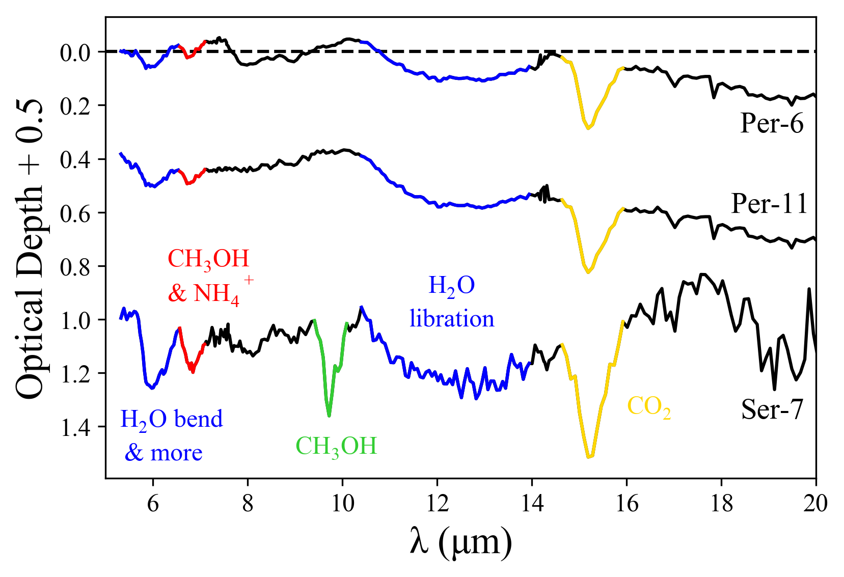
Figure 7: 5-20 $\mu$m optical depth spectra of the targets with the strongest ice absorption features: Per-6, Per-11, and Ser-7, from top to bottom, respectively. A model for the 9.7 $\mu$m and 18 $\mu$m silicate bands has been subtracted. Ice absorption feature identifications are indicated. The 6 $\mu$m and 6.85 $\mu$m absorption features consist of overlapping ice bands, and not all components have been securely identified. The structure between 8-9 $\mu$m toward Per-6 is likely due to insufficiently corrected photospheric absorption. Offsets of 0.5 along the y-axis were applied for clarity.

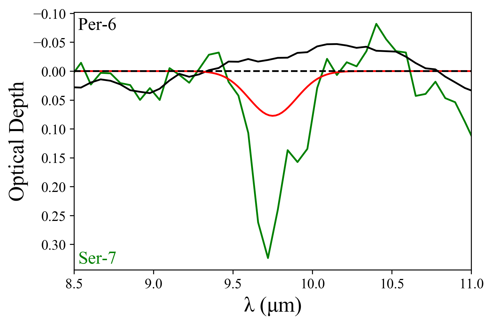
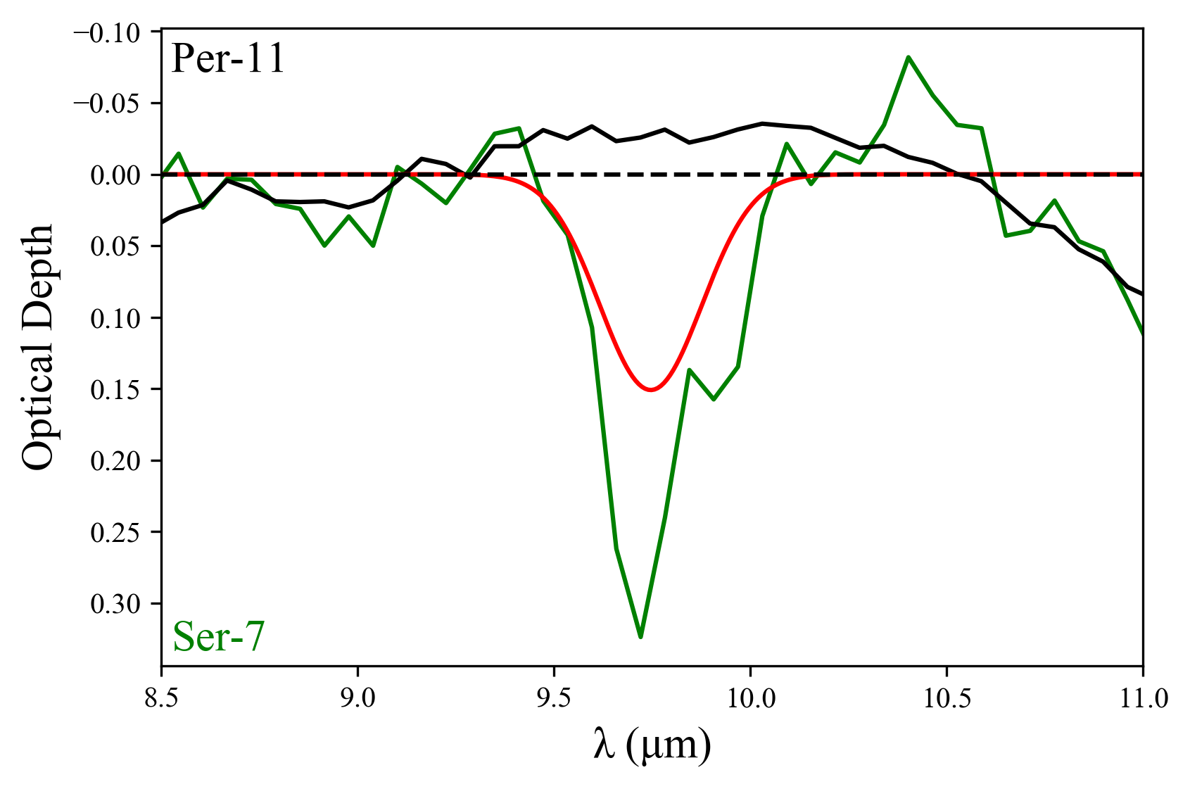
Figure 8: Comparison of the deep $\rm{CH_{3}OH}$ feature in Ser-7 (green) to a selection of other targets with deep 3.0 $\mu$m $\rm{H_{2}O}$ ice bands, Per-6 (left) and Per-11 (right) in black. A model for the 9.7 $\mu$m silicate feature has been subtracted. Ser-7 has an extinction of $A_{\rm K}=4.75\pm 0.44$, Per-6 of $A_{\rm K}=0.75\pm 0.07$, and Per-11 of $A_{\rm K}=1.69\pm 0.07$. Gaussians (red) demonstrate the expected peak depths if the CH₃OH abundance relative to $\rm{H_{2}O}$ were the same in these targets as in Ser-7. CH₃OH is clearly absent, and upper limits are listed in Table 5.

Table 5: CH₃OH Ice Abundances

Alias	$A_{\rm K}$	N($\rm{H_{2}O}$)	N($\rm{CH_{3}OH}$)	$\frac{N(CH_{3}OH)}{N(H_{2}O)}$
	mag	$(10^{17}cm^{-2})$	$(10^{17}cm^{-2})$
Ser-7	4.75$\pm$0.44	26.33$\pm$0.97	5.4$\pm$0.5	0.21$\pm$0.02
Per-6	0.75$\pm$0.07	6.29$\pm$1.36	$<$0.64	$<$0.10
Per-11	1.69$\pm$0.07	13.66$\pm$0.82	$<$0.39	$<$0.03

Note. — The three targets with deep ice bands, as in Fig. 7, including their aliases, extinctions, water ice column densities, methanol column densities, and their methanol to water ice ratios.

5.6 Spatial Context

In order to put the variations in the dust and ice properties observed toward the Perseus and Serpens background stars in a spatial context, we compare them to infrared images, extinction maps, and the YSO population.

We use Spitzer extinction maps and infrared images that were produced by the c2d Legacy project (Evans et al., 2003, 2009). The Perseus extinction map, derived from near-infrared colors, has a resolution of 180” and has a minimum of $A_{\rm V}=2$ mag. For Serpens, the resolution is 90” and starts at the $A_{\rm V}=5$ mag cloud boundary. For the infrared images, we chose the IRAC1 filter at 3.6 $\mu$m, as this is more sensitive to dust scattering than the longer wavelengths. To select the protostellar population, we used the Spitzer c2d catalogs (Evans et al., 2009) available through the InfraRed Sky Archive (IRSA) interface. All Perseus and Serpens targets with infrared spectral indices $\alpha>-0.3$ were selected, where $\alpha$ follows the definition of Lada (1987). These represent the most embedded population of stars. We then designated targets with $-0.3\leq\alpha<0.3$ as “flat spectrum” YSOs, and targets with $\alpha\geq 0.3$ as Class I targets. We also added the more embedded Class 0 sources, that are harder to identify using Spitzer photometry alone due to their weakness. Thirteen Class 0 targets in Perseus were obtained from Jørgensen et al. (2006), and four in Serpens from Hogerheijde et al. (1999). The YSO populations and the background star groups defined by the $\tau_{9.7}$ versus $A_{\rm K}$ correlation (§5.1) are indicated on the IRAC images and extinction maps in Figures 9 and 10 for Perseus and Serpens, respectively.

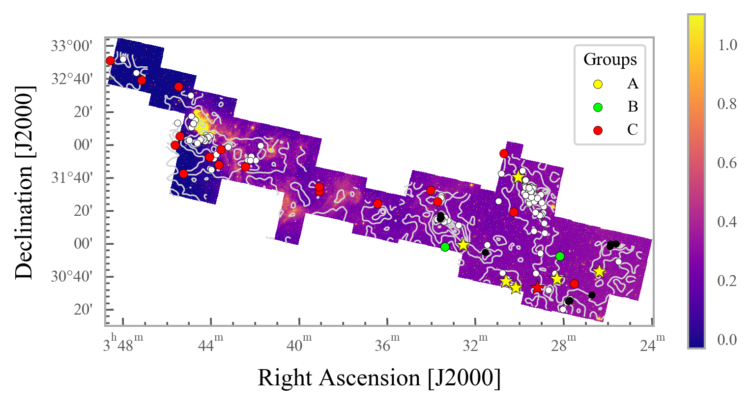
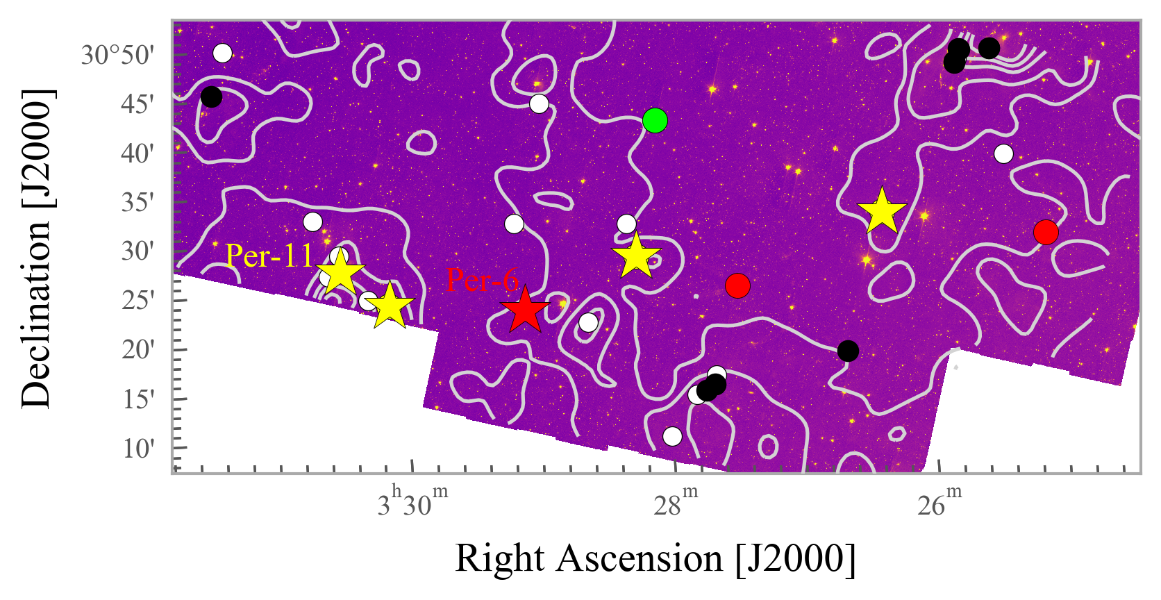
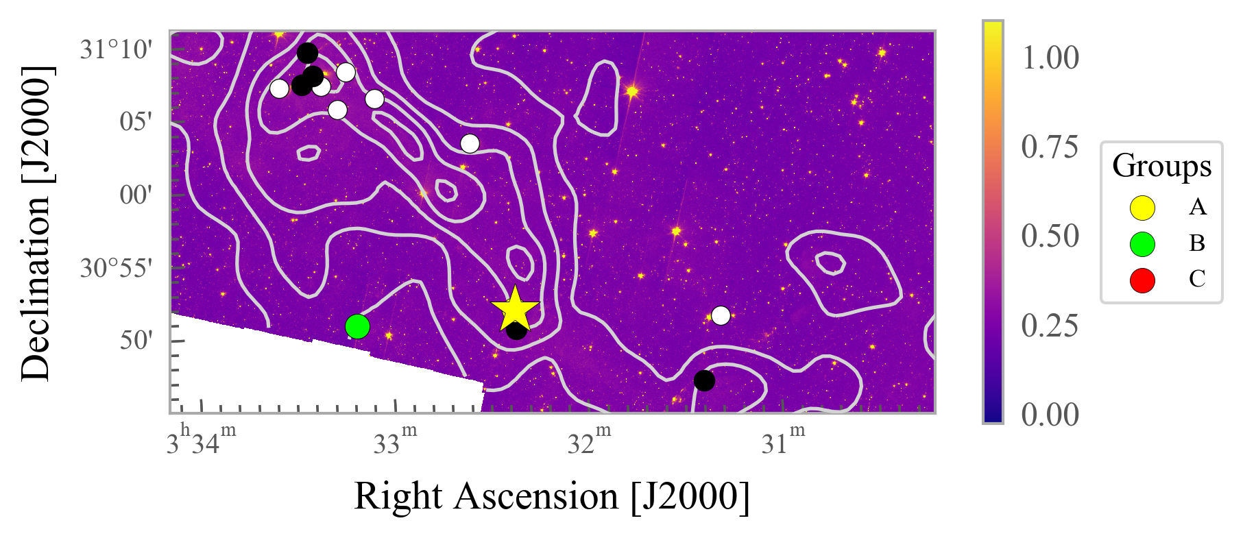
Figure 9: Top panel: Location of the background stars (yellow, green, and red circles and star symbols, as defined in Fig. 3) compared to Class 0 (black) and Class I and “flat spectrum” (white) YSOs observed toward Perseus overlaid the IRAC1 map (3.6 $\mu$m). The colorbar is in units of MJy/sr. The contours represent the extinction map of $A_{\rm V}$ levels of 3, 6, 12, 18, and 24 mag. The star symbols represent the targets that exhibit strong ice features, at $\tau_{3.0}>0.5$ within the uncertainties. Bottom panels: Zoomed in regions of top panel, The red star symbol in the left panel represents Per-6, and the yellow star symbol to the far left Per-11, both of which have particularly deep ice absorption bands.

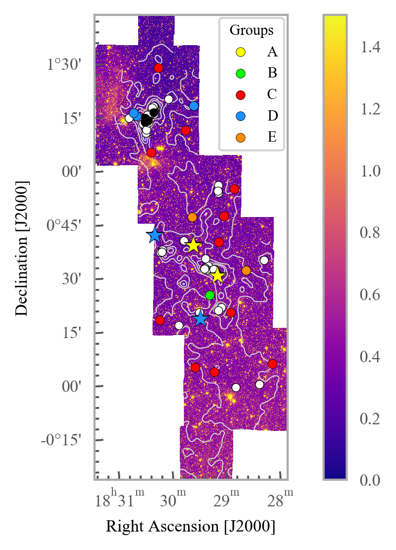
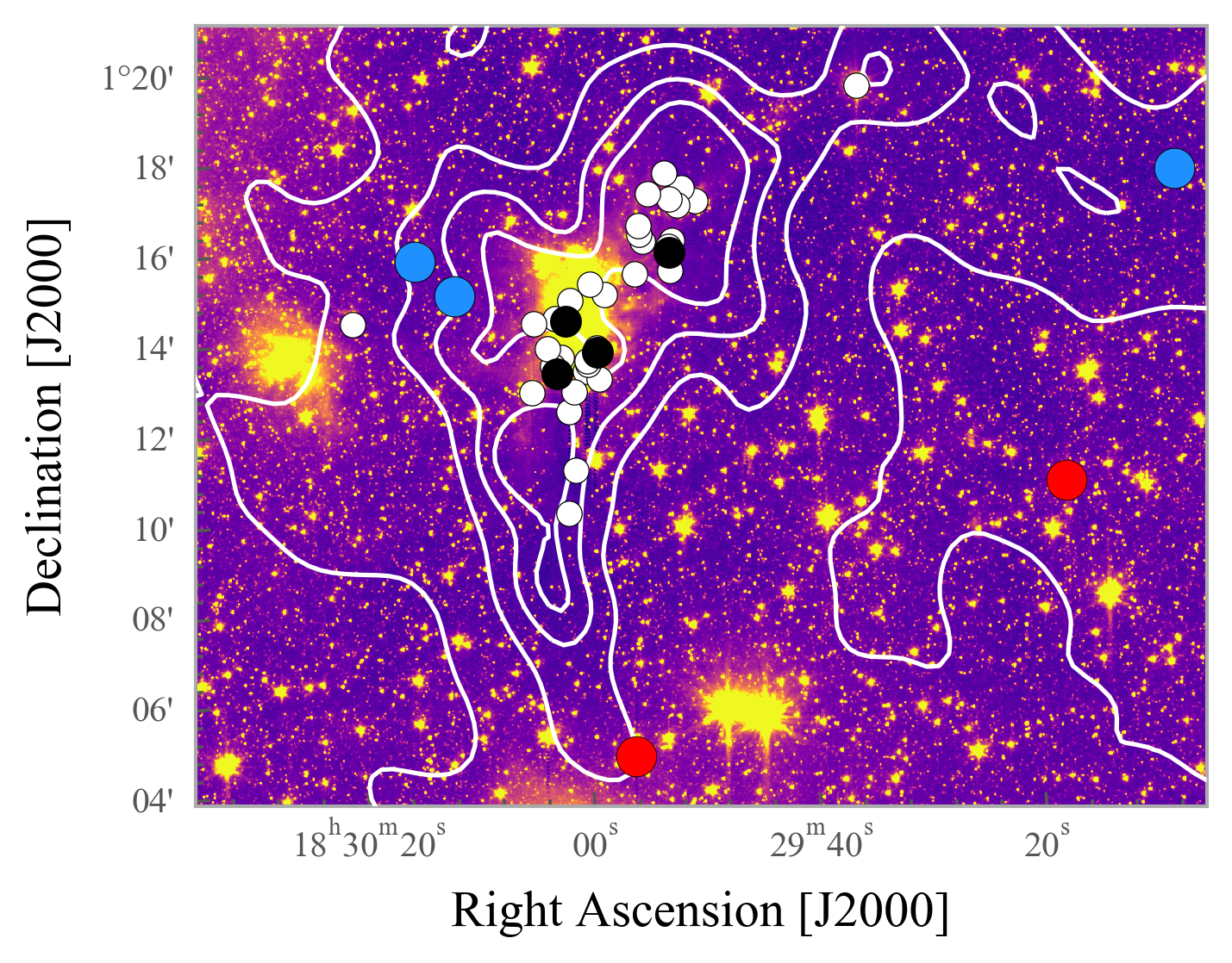
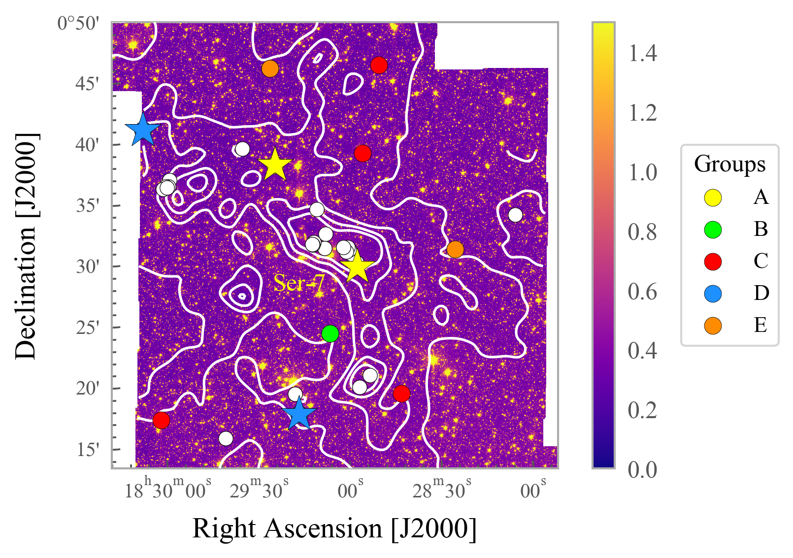
Figure 10: Top panel: Location of the background stars (colored bullets and star symbols, as defined in Fig. 3) compared to Class 0 (black) and Class I and “flat spectrum” (white) YSOs observed toward Serpens overlaid the IRAC1 map (3.6 $\mu$m). The colorbar is in units of MJy/sr. The contours represent the extinction map of $A_{\rm V}$ levels of 3, 6, 12, 18, and 24 mag. The star symbols represent the targets that exhibit strong ice features, at $\tau_{3.0}>0.5$ within the uncertainties Bottom panels: Zoomed in regions for known clusters in Serpens, the “core” (left) and “Ser/G3-G6” (right). The yellow asterisk near the center represents Ser-7, which exhibits particularly strong ice features.

For Perseus, the majority of the Group A (“dense” cloud-type) targets are located in the Western portion of the cloud (Fig. 9). This is also where the five Class 0 YSOs are all located. Class 0 envelopes extend to typically 1 arcmin in Perseus (Enoch et al., 2006). Group A target Per-9 is located 143” (35,631 AU) from the Class I YSO IRAS 03271+3013. Another Group A target, Per-12, is located 67” (16,819 AU) from the Class 0 YSO IRAS 03292+3039. The smallest distance is 53” between the background star Per-11 and the Class 0 target [DCE2008] 081, and, therefore, it appears that none of the background stars significantly trace Class 0 envelopes.

It is noteworthy that the two Group B (“diffuse ISM-like”) targets are located in the Western part of Perseus as well. They are located at the edges of extinction enhancements, and somewhat further away from YSOs compared to several Group A targets. The number of targets is small, however, and these trends are not statistically significant. The median distance between the six Group A targets and nearest YSOs is 176” with a standard deviation of 240”; the distances of the two Group B targets and their nearest YSOs are 657” and 671”.

The Perseus targets with the deepest ice bands, Per-6 (Group C) and Per-11 (Group A), are also located in the Western region of Perseus. Per-11 is located among a small cluster of Class I and “flat spectrum” YSOs, but Per-6 is also located near such YSOs. Overall, these results indicate a significant variety of dust properties within Perseus. Dense-cloud like dust is found within the vicinity ($\sim$15,000 AU) of YSOs but also in regions without YSOs. Diffuse ISM-like dust may have strong ice absorption, and is also found in the denser regions.

In Serpens, most of the Class I and “flat spectrum” YSOs are concentrated in two clusters, one located in the upper half of Serpens, and the other, “Ser/G3-G6,” located around the middle of the molecular cloud (Zhang et al., 1988). The four Class 0 YSOs are toward the center of the upper cluster (Fig. 10). The Group A target Ser-7 is located at the edge of Ser/G3-G6, but within an arcminute of the YSO cluster. Ser-7 has very deep ice bands, and a very large $\rm{CH_{3}OH}$ ice abundance. This likely reflects a high density associated with the star formation in this cluster. The single Group B target is located in a local extinction minimum. Group D targets (intermediate between “diffuse ISM-like” and “dense-like” dust) are spread out along the molecular cloud, in some cases located near the edges of local cores or near YSOs, but certainly not in all cases.

Overall, as for Perseus, no clear correlations stand out for Serpens, and the dust properties are governed by local physical conditions not evident in these tracers. The distances between the two Group A targets and their nearest YSOs are 180” (standard deviation 23”); for the one Group B target, there is a distance of 285”; and for the six Group D targets, there is a median distance of 118” with a standard deviation of 105”.

6 Discussion

6.1 The $A_{\rm K}$/$\tau_{9.7}$ Ratio in Grain Growth Models

Grain growth, starting when most grains are much smaller than the near-infrared wavelength, i.e., in the Rayleigh limit, will increase $A_{\rm K}$ initially. But when the grain sizes become comparable to or larger than $\sim 0.4$ $\mu$m ($\lambda/2\pi$), gray extinction becomes important, and $A_{\rm K}$ (per dust mass), derived from the near-IR color excess, will decrease. This implies that the observed $A_{\rm K}$/$\tau_{9.7}$ reduction in dense clouds (Fig. 3) could trace a moderate amount of grain growth. This is also concluded by Ormel et al. (2011) based on grain growth models. These models further infer that the grain growth is in the form of aggregates of ice coated silicate and ice coated carbonaceous grains. The increased stickiness of ice coated grains is key in the coagulation process. The observed relation between $A_{\rm K}$/$\tau_{9.7}$ and the ices ($\tau_{3.0}$) will be discussed in §6.2.

Such moderate grain growth is consistent with the invariant profiles of the 9.7 $\mu$m absorption bands. This was also the primary conclusion of the extensive study by Van Breemen et al. (2011). The coagulated grains are too small to affect the profile of the 3.0 $\mu$m ice band as well, as little variation is observed as a function of extinction (Fig. 11). The long-wavelength wing, which is thought to be affected by large grain scattering, limits the grains to sizes of $\frac{3}{2\pi}\approx$ 0.5 $\mu$m and less. Some variation is observed on the short wavelength wing, which might be a result of NH₃ abundance variations due to the N-H stretching mode at 2.9 $\mu$m. Indeed, the target with the strongest short-wavelength wing also shows a more pronounced 3.47 $\mu$m feature, which results from ammonia hydrates (Dartois & d’Hendecourt, 2001).

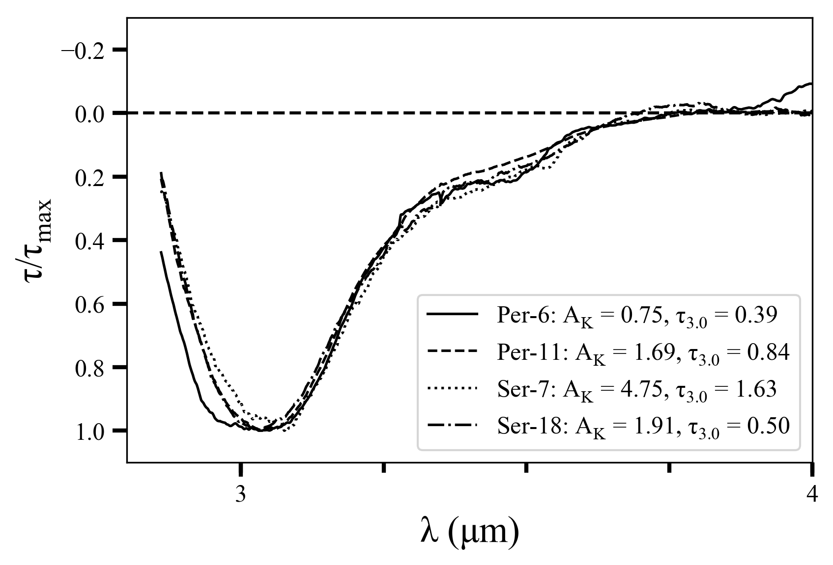
Figure 11: Profile of the 3 $\mu$m water ice bands observed toward four targets tracing a range of extinctions ($A_{K}=0.75-4.75$). Per-6 is Group C, Per-11 is Group A, Ser-7 is Group A, and Ser-18 is Group D. The spectra have been normalized and smoothed to a resolving power of 100. Little variation is evident in the long-wavelength wing, indicating insignificant growth of the relative population of grains larger than $\sim$0.5.

A different scenario was discussed in Chiar et al. (2007) and Ormel et al. (2011). Considering that the $K-$band extinction is primarily caused by carbonaceous grains, the reduction of the $\tau_{9.7}$/$A_{\rm K}$ ratio (Fig. 3) is possible if growth is limited to silicate grains in the inner cloud regions. These grains would need to be much larger than 1 $\mu$m so that they do not contribute to the $\tau_{9.7}$ absorption feature (and also not to $A_{\rm K}$), and not change its profile. In the models of Ormel et al. (2011), the silicate absorption feature disappears for time scales longer than 1 Myr at a density of 10⁵ cm^-3, or at shorter time scales at higher densities. Thus, in this scenario, large ice-rich silicate grains reside in the inner, dense regions of the clouds, while the small silicate grains in the outer regions are responsible for the 9.7 $\mu$m absorption feature. Carbonaceous grains would not form such large grains, perhaps due to not acquiring ice mantles. It is unclear why this would be the case. In fact, the increase of $\tau_{3.0}$ as a function of $A_{\rm K}$, as observed in both Perseus and Serpens (Fig. 4), is difficult to explain with ice-less carbonaceous grains. If only silicate grains, tracing the outer cloud layers, are covered with ice mantles, the $\tau_{3.0}$ as a function of $A_{\rm K}$ would flatten, which is clearly not the case. Thus, overall, this scenario seems less likely.

6.2 $A_{\rm K}$/$\tau_{9.7}$ Variations and Relations with Ices and Dense Core Formation

Striking variations in the relation between $A_{\rm K}$ and $\tau_{9.7}$ are observed (Fig. 3). At the highest extinctions, the targets are trending to lie systematically below the linear fit, i.e., $\tau_{9.7}$ is suppressed relative to $A_{\rm K}$. For Perseus, this inflection occurs at $A_{\rm K}\sim 1.2$ ($A_{\rm V}\sim 10$, assuming $A_{\rm V}$/$A_{\rm K}$ = 8.4), while for Serpens, it is near $A_{\rm K}\sim 2$ ($A_{\rm V}\sim 17$). Below this inflection point, the data points are located between the diffuse and dense cloud relations. Above this inflection point, the data points tend to follow the dense cloud relation. The same is observed for the third cloud in our survey, Lupus, which shows an inflection point similar to Perseus (Boogert et al., 2013).

In Fig. 12, we accumulate all $\tau_{9.7}$ and $A_{\rm K}$ data of other clouds and cores known to us (Chiar et al., 2007; Boogert et al., 2011, 2013). In addition to Perseus, Serpens, and Lupus (I and IV), this includes targets tracing Taurus, IC 5146, Barnard 68, Chameleon I, and a range of isolated dense cores. The isolated dense cores extend the $A_{\rm K}$ range to much higher values. An overall correlation is visible, but the scatter is large. The fitted line to all the data lies between the diffuse ISM and dense core correlations, just as for our individual cloud fits. An overall inflection point, after which the targets center around the dense cloud correlation, is also visible, near $A_{\rm K}\sim 1.5$ ($A_{\rm V}\sim 13$). Thus, overall, assuming that the $\tau_{9.7}/A_{\rm K}$ ratio is a measure of grain sizes (§6.1), Fig. 12 shows that the dust coagulation process follows a smilar pattern across different clouds.

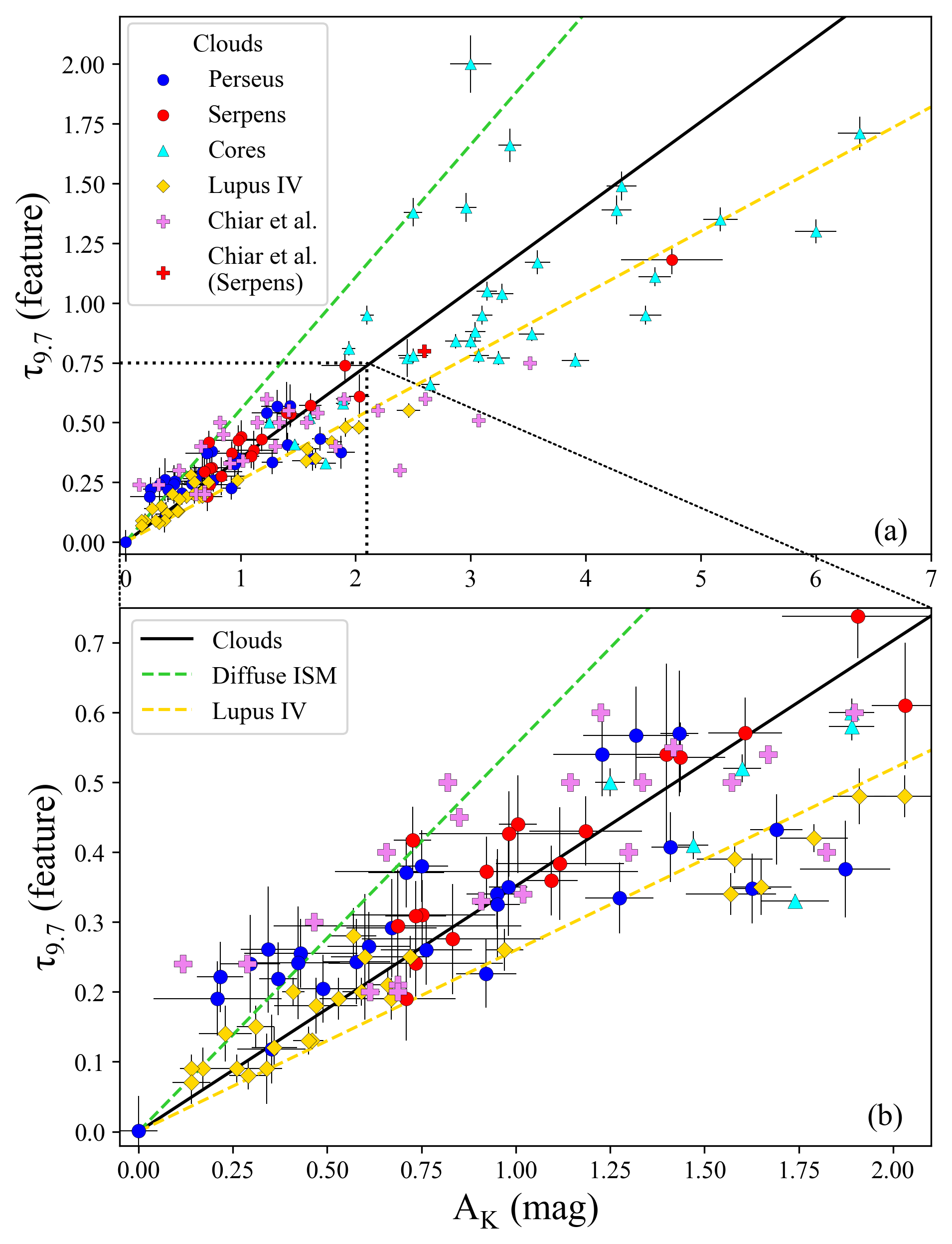
Figure 12: Silicate ice and extinction correlation for the Perseus, Serpens, Lupus, Taurus, and Chameleon I molecular clouds, as well as several dense cores, taken from Chiar et al. (2007), and Boogert et al. (2011, 2013). The bottom panel zooms in on the lower extinctions. The data points are color-coordinated by cloud, as indicated. The black line is the linear fit to all targets. The green dotted line is the diffuse ISM correlation (Whittet, 2003), and the yellow dotted line is the Lupus IV correlation (Boogert et al., 2011). The error bars, when available, are 3$\sigma$. Four Lupus IV sources have upper limits that are consistent with the general correlation but are not included in this graph. The isolated dense core targets near the diffuse ISM relation trace L328, which is thought to be strongly contaminated by foreground dust absorption.

It does appear that these $\tau_{9.7}$/$A_{\rm K}$ variations relate to the ice band optical depths. For Perseus, the $\tau_{3.0}$ values for Group A targets (lowest $\tau_{9.7}$/$A_{\rm K}$) are significantly higher compared to all other targets, even those at similar $A_{\rm K}$ (Fig. 4). Indeed, the Group A targets are well separated in the $\tau_{9.7}$/$A_{\rm K}$ versus $\tau_{3.0}$ correlation plots (Fig. 6). The Lupus cloud shows a similar behavior. For Serpens, targets with the largest $\tau_{9.7}$/$A_{\rm K}$ ratios, have the largest $\tau_{3.0}$ values, although very few lines of sight with deep 3.0 $\mu$m ice bands are available.

The threshold for ice formation is similarly low for all clouds ($A_{\rm V}\sim 2.6-3.4$; §6.3), and thus it appears that not only the mere presence of ice on the grains, but also the ice column density (traced by $\tau_{3.0}$) is an important factor in the grain growth process. This, in turn, relates to the cloud density, as lines of sight with deeper ice bands, likely trace higher densities deeper into the cloud.

Indeed, for both scenarios discussed in §6.1, the $\tau_{9.7}$ versus $A_{\rm K}$ relation is a measure of the density structure of the clouds. The inflection point in this relation reflects a transition to higher density inner cloud regions where grain growth accelerates. This implies that the density structure for Serpens is shallower than for Perseus, Lupus, and other dense cores, although the density at the cloud edge is similar for all these clouds, as evidenced by their similar ice formation thresholds (§6.3). Within Perseus, however, coagulation is strongest for the targets with the largest ice column densities.

In addition to the overall trends described above, there are deviations, indicating that local conditions, such as density fluctuations, across the cloud also matter. Such local scatter in the $\tau_{9.7}$ versus $A_{\rm K}$ plots was also noted for Lupus (Boogert et al., 2013). Fig. 13 compares the optical depth spectra of Per-19 (Group C) and Per-2 (Group A), which have similar $A_{\rm K}$ values, but Per-19 has a 50% deeper 9.7 $\mu$m silicate band. Conforming with its diffuse ISM nature, Per-19 has a factor of $\sim$2.5 less water ice than Per-2. Thus, Per-19 appears to trace lower density cloud material. In contrast, Ser-19 and Ser-6 have similar $\tau_{9.7}$ and $A_{\rm K}$ at very different $\tau_{3.0}$ (Fig. 14). Ser-19 is in fact the only Serpens target without ice. It is relatively isolated on the edge of the cloud, but it is unclear if this plays a role. Unfortunately, Ser-19 and Ser-6 have uncertainn $\tau_{9.7}/A_{\rm K}$ ratios (Group C), precluding a distinction between dense-like (Group A) or diffuse-like (Group B) dust.

It is worthwhile to note that the inflection points in the $A_{\rm K}$ versus $\tau_{9.7}$ relation of $A_{\rm V}\sim 10$ and $A_{\rm V}\sim 17$ for Perseus and Serpens, respectively, are comparable to the dense core formation thresholds in these clouds. Enoch et al. (2007) derive dense core formation thresholds of $A_{\rm V}\sim 8$ and $A_{\rm V}\sim 15$ from comprehensive infrared and sub-millimeter surveys. This reinforces the idea that the dust coagulation process is enhanced at higher densities.

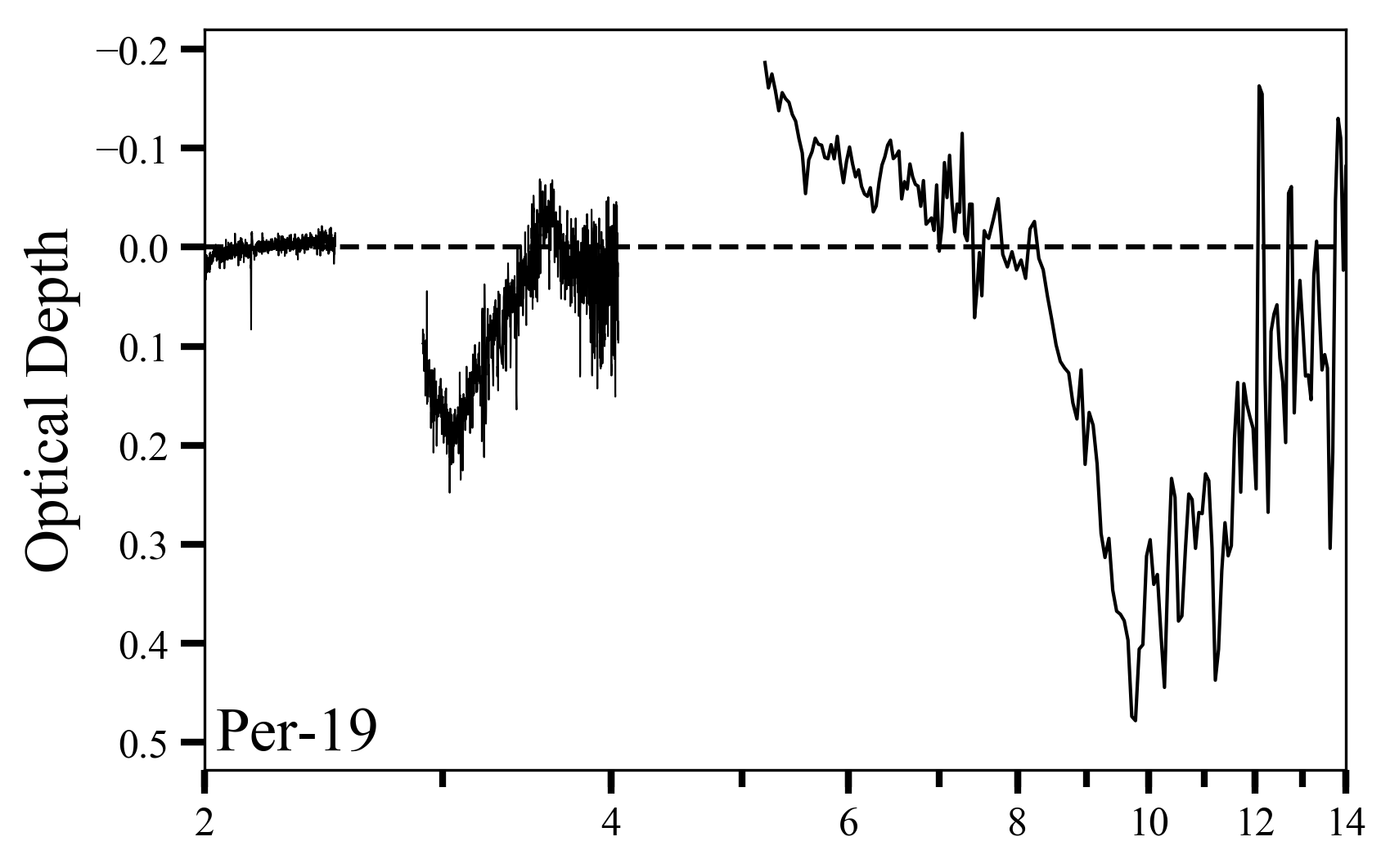
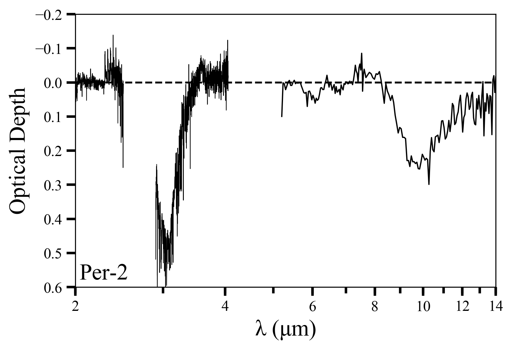
Figure 13: Comparison of the 3.0 and 9.7 $\mu$m ice and silicate bands of the targets Per-19 and Per-2. Both targets have similar $A_{\rm K}$ values, but Per-19 has a much deeper 9.7 $\mu$m silicate band (and thus belongs to “diffuse ISM” Group B). Conforming with its diffuse ISM nature, Per-19 has a factor of $\sim$2.5 less water ice than Per-2, as seen by the shallower 3.0 $\mu$m $\rm{H_{2}O}$ feature. Such variations might point to a relation between ice formation and grain coagulation. The negative optical depth values between 5-8 $\mu$m for Per-19 are due to the choise of a local baseline for the 9.7 $\mu$m absorption feature, as noted in Table 3.

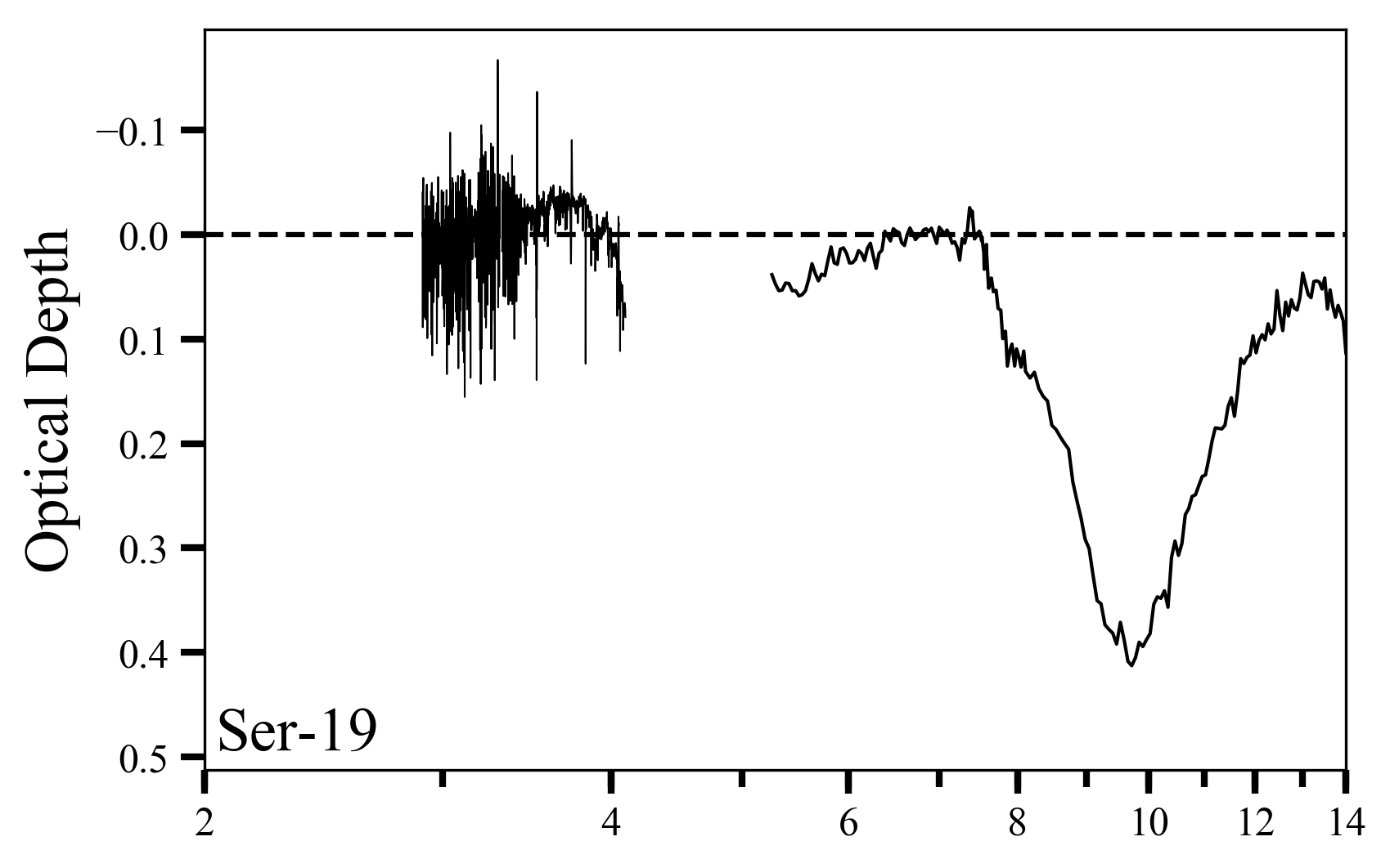
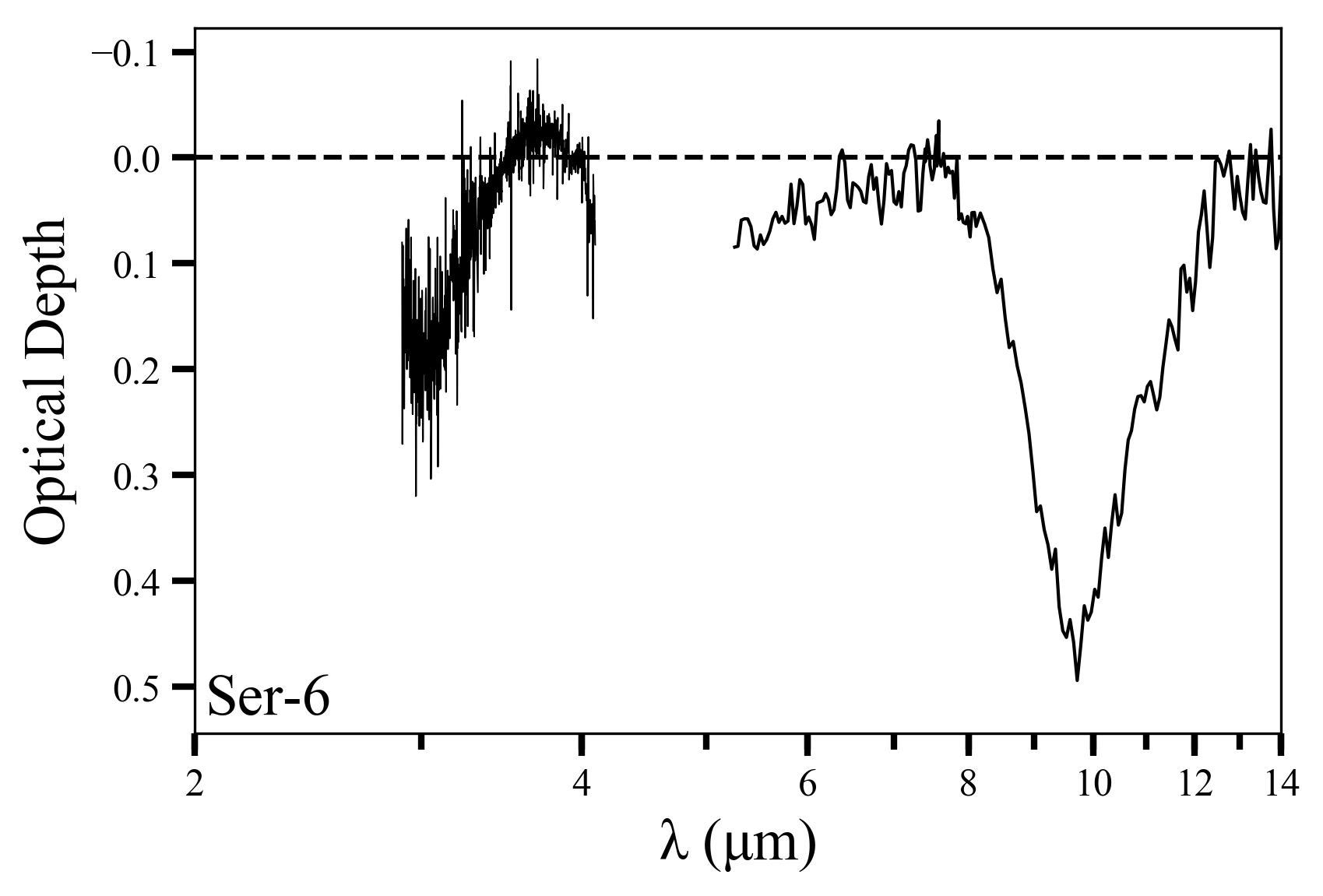
Figure 14: The targets Ser-19 and Ser-6 have similar $A_{\rm K}$ values and 9.7 $\mu$m silicate band depths, but only Ser-6 displays the 3.0 $\mu$m $\rm{H_{2}O}$ feature. The $L$-band portions have been smoothed to a resolving power of 25. This comparison indicates that ice formation is not the only factor that affects coagulation as traced by the $A_{\rm K}$/$\tau_{9.7}$ ratio.

6.3 Ice Formation Threshold

The relation between $A_{\rm K}$ and $\tau_{3.0}$ (§5.2, Fig. 4) for Serpens shows a cut-off along the $A_{\rm K}$ axis of $0.616\pm 0.087$ ($A_{V}=5.17\pm 0.06$), which is approximately twice that of Perseus ($A_{V}=2.65\pm 0.25$), Lupus IV ($A_{V}=2.10\pm 0.59$; Boogert et al. 2011), and Taurus ($A_{V}=3.2\pm 0.1$; Whittet et al. 2001). This might be attributed to extinction by unrelated foreground dust. Serpens is located at a larger distance ($420\pm 15$ pc) than all these other clouds: $294\pm 15$ pc for Perseus, $141\pm 7$ pc for Taurus, and $189\pm 13$ pc for Lupus (Ortiz-León et al., 2018; Zucker et al., 2019). To the first order, the foreground extinction due to diffuse dust in the Galactic Plane may be estimated by scaling to the extinction of $A_{\rm V}\sim 30$ towards the Galactic Center (Rieke et al. 1989 and references therein) at $\sim 8$ kpc. This results in foreground contributions of $A_{\rm V}\sim 1.6$, 1.1, 0.7, and 0.5 mag for Serpens, Perseus, Lupus IV, and Taurus, respectively. Models using Gaia-derived distances (Zucker et al., 2019), however, point to a larger foreground contribution ($A_{\rm V}=3.0$) for Serpens than for all the other clouds ($A_{\rm V}=1.0)$. This could be related to its location closer to the Galactic Plane ($b\sim+4^{\circ}$), more directed to the Galactic Center ($l\sim 30^{\circ}$) than the other clouds.

Overall, when correcting for the larger foreground extinction towards Serpens, it thus seems that H₂O ice is formed at similar depths for all studied clouds. This would be at $A_{\rm V}\sim 2.6-3.4$, or $\sim 1.6-2.4$ when subtracting the 1.0 mag foreground for all (Zucker et al., 2019). If we further correct for the fact that the observations trace both the front and back of the clouds, the cloud depth at which H₂O ice is abundantly formed is $A_{Vf}\sim 0.8-1.2$ mag. Following Hollenbach et al. (2009), this could indicate that the cloud edges have similar densities ($n$), provided that they experience similar interstellar radiation fields $F_{0}G_{0}$

$$A_{Vf}=0.56\times ln\left(\frac{G_{0}F_{0}Y}{n(O)\nu_{0}}\right)$$ (6)

where Y is the total yield of photodesorbing $\rm{H_{2}O}$ ice, and $\nu_{O}$ is the vibrational frequency of O atoms bound to a grain surface related to dust temperature. For typical conditions (Hollenbach et al., 2009), this corresponds to $n\sim 3\times 10^{4}$ at $A_{Vf}\sim 0.8-1.2$ mag

A higher threshold was observed toward the Ophiuchus cloud (Tanaka et al., 1990) and is usually ascribed to the presence of a nearby O and B-stars, increasing $F_{0}$, photodesorbing the ices. No such sources for a high UV radiation field near the other clouds are known. Note that if the larger cut-off in the relation between $A_{\rm K}$ and $\tau_{3.0}$ is not caused by foreground dust, Eq. 6 would imply a lower Serpens cloud edge density compared to the other clouds by a factor of $\sim$7.

6.4 $\rm{CH_{3}OH}$

One of our targets, Ser-7, shows a very high $\rm{CH_{3}OH}$ abundance of $\sim$21% relative to $\rm{H_{2}O}$, surpassing previous records for background stars of L694 ($\sim$14%; Chu et al., 2020) and L429-C ($\sim$12%; Boogert et al., 2011). This target was also noted as containing high abundances of other organic molecules, such as methane ($\rm{CH_{4}}$), and, tentatively, solid acetylene ($\rm{C_{2}H_{2}}$) at 13.5 $\mu$m (Knez et al., 2008, 2012).

The $\rm{CH_{3}OH}$ abundance toward Ser-7 is significantly larger than the upper limits derived for other Serpens and Perseus background stars (Fig. 8). It approaches the largest CH₃OH ice abundances observed toward YSOs in Serpens (28%; Pontoppidan et al. 2004; Perotti et al. 2020). Of all background stars in our sample, Ser-7 is closest to a YSO (2MASSJ18285277+0028463), which is a member of the Ser/G3-G6 cluster of Class I and “flat spectrum” YSOs. At an angular distance of 23” (5,725 AU), the large CH₃OH abundance might trace the very outer edges of the envelope of this flat spectrum YSO, or the high density core material within which the cluster formed. While $\rm{CH_{3}OH}$ is also expected to form at low densities (e.g., Qasim et al. 2018), its formation is strongly enhanced at high densities ($10^{5}$ cm^-3) when CO rapidly freezes out (Cuppen et al., 2009). Indeed, so far all CH₃OH ice detections toward background stars trace sightlines with very high extinction, above a threshold of $A_{\rm V}\sim 18$ ($A_{\rm K}\sim 2$; Boogert et al. 2015; Chu et al. 2020). Ser-7 is the only target in our Serpens and Perseus sample with an extinction ($A_{\rm K}=4.75\pm 0.44$) above this threshold.

7 Summary and Future Work

We present 2-4 and 5-20 $\mu$m spectra of a sample of 28 stars behind the Perseus and 21 stars behind the Serpens molecular clouds. We fitted the target spectra using a combination of template spectra from the IRTF spectral database and photospheric model spectra, combined with extinction curves, laboratory $\rm{H_{2}O}$ ice spectra, and silicate absorption spectra to derive $A_{\rm K}$, $\tau_{3.0}$, and $\tau_{9.7}$ values. Correlation plots of $\tau_{9.7}$ versus$A_{\rm K}$ show a variation of a factor of $\sim$2 for both clouds. Combining our $\tau_{9.7}$ and $A_{\rm K}$ values with those available in the literature indicates that such scatter is common.

In general, the $\tau_{9.7}$/$A_{\rm K}$ ratios are reduced relative to the diffuse ISM. The largest reductions, up to a factor of 2, are visible above $A_{K}\sim$1.2 for Perseus and Lupus, and above $A_{K}\sim 2.0$ for Serpens. A picture emerges that grains, after acquiring ice mantles (at $A_{K}\sim$0.2-0.4), grow to moderate sizes due to higher densities deeper in the cloud, especially above $A_{K}\sim$1.2-2. A significant population of grains larger than $\sim 0.5$ $\mu$m is unlikely, however, as this would increase the $\tau_{9.7}$/$A_{\rm K}$ ratio, and would also change the profiles of the 3.0 and 9.7 $\mu$m absorption profiles, which is not observed.

The regions with the lowest $\tau_{9.7}$/$A_{\rm K}$ ratios are also the regions where dense core (and thus star) formation will take place, considering similar dense core formation extinction thresholds. Indeed, Serpens stands out by having a factor of $\sim$2 higher inflection in the $\tau_{9.7}$ versus $A_{\rm K}$ relation, and also a factor of 2 larger dense core formation threshold. These aspects may indicate that Serpens has an overall shallower density profile than the other clouds.

We derived H₂O ice formation thresholds of $A_{\rm V}\sim 2.6-3.4$ for all studied clouds, after correction for a 2 mag larger foreground extinction towards Serpens. This threshold is well below the extinctions where the lowest $\tau_{9.7}$/$A_{\rm K}$ ratios are observed. Thus we conclude that, in agreement with the grain growth models by Ormel et al. (2011), grain coagulation is facilitated by ice mantles, and enhanced at higher densities. Targets tracing the highest ice column densities (proportional to $\tau_{3.0}$), and thus likely densities, have the lowest $\tau_{9.7}/A_{\rm K}$ ratios.

Besides the overall trends, we also found a large scatter in the $\tau_{9.7}$/$A_{\rm K}$ ratio across small $A_{\rm K}$ intervals. Using extinction maps, infrared images, YSO and molecular outflow locations, we did not find strong correlations of these variations with cloud location. Finally, we found three targets (Per-6, Per-11, Ser-7) with particularly deep ice bands, of which Ser-7 has an especially high $\rm{CH_{3}OH}$ ice abundance of 21% relative to $\rm{H_{2}O}$. This is significantly higher than the upper limits in the other sources, which is attributed to high densities in a local star formation region.

A larger sample of sight-lines, fully covering a wide range of $A_{\rm K}$ values and molecular cloud conditions is needed to further constrain the relation between ice formation, the silicate band, and continuum extinction. A confirmation of the inflection in the $A_{\rm K}$ versus $\tau_{9.7}$ relation is needed, as well as studies of the origin of the scatter in the $\tau_{9.7}/A_{K}$ ratio, in particular the relation with local density. Future work will rely heavily on observations with the James Webb Space Telescope (JWST), enabling the construction of detailed maps of $A_{\rm K}$, $\tau_{3.0}$, and $\tau_{9.7}$, facilitating an assessment of the relation between grain coagulation and other cloud properties.

8 Acknowledgments

We thank Lee Mundy and Ewine van Dishoeck for their help with the early stages of this project. We thank Megan Kiminki who worked on this project while an REU student at the SETI Institute, supported by NSF grant AST-1359346. MCLM thanks the Institute for Astronomy at UH Manoa for their hospitalty, and Columbia University in the City of New York and the I.I. Rabi Scholars Program for their generous financial support. We thank the referee for insightful comments, in particular on the cloud distances and foreground extinction correction, that helped improve this paper. This work is based on observations made at the IRTF and Keck telescopes. We wish to extend our special thanks to those of Hawaiian ancestry on whose sacred mountain of Maunakea we are privileged to be guests. The observations presented herein would not have been possible without their generosity. The authors recognize that the summit of Maunakea has always held a very significant cultural role for the indigenous Hawaiian community. We are thankful to have the opportunity to use observations from this mountain.

9 Appendix

Figure 15: (Continuation)

Figure 15: (Continuation)

Figure 15: (Continuation)

Figure 15: (Continuation)

Figure 15: (Continuation)

Figure 15: (Continuation)

Figure 15: (Continuation)

Figure 15: (Continuation)

Figure 15: (Continuation)

Figure 15: (Continuation)

Figure 15: (Continuation)

Figure 15: (Continuation)

Figure 15: (Continuation)

Figure 15: (Continuation)

References

- Boogert et al. (2013) Boogert, A. C. A., Chiar, J. E., Knez, C., et al. 2013, ApJ, 777, 73, doi: 10.1088/0004-637X/777/1/73
- Boogert et al. (2015) Boogert, A. C. A., Gerakines, P. A., & Whittet, D. C. B. 2015, ARA&A, 53, 541, doi: 10.1146/annurev-astro-082214-122348
- Boogert et al. (2008) Boogert, A. C. A., Pontoppidan, K. M., Knez, C., et al. 2008, ApJ, 678, 985, doi: 10.1086/533425
- Boogert et al. (2011) Boogert, A. C. A., Huard, T. L., Cook, A. M., et al. 2011, ApJ, 729, 92, doi: 10.1088/0004-637X/729/2/92
- Cambrésy et al. (2011) Cambrésy, L., Rho, J., Marshall, D. J., & Reach, W. T. 2011, A&A, 527, A141, doi: 10.1051/0004-6361/201015863
- Chiar et al. (1996) Chiar, J. E., Adamson, A. J., & Whittet, D. C. B. 1996, ApJ, 472, 665, doi: 10.1086/178097
- Chiar et al. (2007) Chiar, J. E., Ennico, K., Pendleton, Y. J., et al. 2007, ApJ, 666, L73, doi: 10.1086/521789
- Chu et al. (2020) Chu, L. E. U., Hodapp, K., & Boogert, A. 2020, ApJ, 904, 86, doi: 10.3847/1538-4357/abbfa5
- Cuppen et al. (2009) Cuppen, H. M., van Dishoeck, E. F., Herbst, E., & Tielens, A. G. G. M. 2009, A&A, 508, 275, doi: 10.1051/0004-6361/200913119
- Cushing et al. (2004) Cushing, M. C., Vacca, W. D., & Rayner, J. T. 2004, PASP, 116, 362, doi: 10.1086/382907
- Dartois & d’Hendecourt (2001) Dartois, E., & d’Hendecourt, L. 2001, A&A, 365, 144, doi: 10.1051/0004-6361:20000174
- Decin et al. (2004) Decin, L., Morris, P. W., Appleton, P. N., et al. 2004, ApJS, 154, 408, doi: 10.1086/422884
- Enoch et al. (2007) Enoch, M. L., Glenn, J., Evans, Neal J., I., et al. 2007, ApJ, 666, 982, doi: 10.1086/520321
- Enoch et al. (2006) Enoch, M. L., Young, K. E., Glenn, J., et al. 2006, The Astrophysical Journal, 638, 293, doi: 10.1086/498678
- Evans et al. (2003) Evans, Neal J., I., Allen, L. E., Blake, G. A., et al. 2003, PASP, 115, 965, doi: 10.1086/376697
- Evans et al. (2009) Evans, Neal J., I., Dunham, M. M., Jørgensen, J. K., et al. 2009, ApJS, 181, 321, doi: 10.1088/0067-0049/181/2/321
- Gibb et al. (2004) Gibb, E. L., Whittet, D. C. B., Boogert, A. C. A., & Tielens, A. G. G. M. 2004, ApJS, 151, 35, doi: 10.1086/381182
- Harvey et al. (2006) Harvey, P. M., Chapman, N., Lai, S.-P., et al. 2006, ApJ, 644, 307, doi: 10.1086/503520
- Hogerheijde et al. (1999) Hogerheijde, M. R., van Dishoeck, E. F., Salverda, J. M., & Blake, G. A. 1999, ApJ, 513, 350, doi: 10.1086/306844
- Hollenbach et al. (2009) Hollenbach, D., Kaufman, M. J., Bergin, E. A., & Melnick, G. J. 2009, ApJ, 690, 1497, doi: 10.1088/0004-637X/690/2/1497
- Hudgins et al. (1993) Hudgins, D. M., Sandford, S. A., Allamandola, L. J., & Tielens, A. G. G. M. 1993, ApJS, 86, 713, doi: 10.1086/191796
- Indebetouw et al. (2005) Indebetouw, R., Mathis, J. S., Babler, B. L., et al. 2005, ApJ, 619, 931, doi: 10.1086/426679
- Jørgensen et al. (2006) Jørgensen, J. K., Harvey, P. M., Evans, Neal J., I., et al. 2006, ApJ, 645, 1246, doi: 10.1086/504373
- Keane et al. (2001) Keane, J. V., Tielens, A. G. G. M., Boogert, A. C. A., Schutte, W. A., & Whittet, D. C. B. 2001, A&A, 376, 254, doi: 10.1051/0004-6361:20010936
- Kerkhof et al. (1999) Kerkhof, O., Schutte, W. A., & Ehrenfreund, P. 1999, A&A, 346, 990
- Knez et al. (2012) Knez, C., Moore, M. H., Ferrante, R. F., & Hudson, R. L. 2012, ApJ, 748, 95, doi: 10.1088/0004-637X/748/2/95
- Knez et al. (2008) Knez, C., Moore, M., Travis, S., et al. 2008, in Organic Matter in Space, ed. S. Kwok & S. Sanford, Vol. 251, 47–48, doi: 10.1017/S1743921308021157
- Lada (1987) Lada, C. J. 1987, in Star Forming Regions, ed. M. Peimbert & J. Jugaku, Vol. 115, 1
- McClure (2009) McClure, M. 2009, ApJ, 693, L81, doi: 10.1088/0004-637X/693/2/L81
- McLean et al. (1998) McLean, I. S., Becklin, E. E., Bendiksen, O., et al. 1998, in Society of Photo-Optical Instrumentation Engineers (SPIE) Conference Series, Vol. 3354, Infrared Astronomical Instrumentation, ed. A. M. Fowler, 566–578, doi: 10.1117/12.317283
- Ormel et al. (2011) Ormel, C. W., Min, M., Tielens, A. G. G. M., Dominik, C., & Paszun, D. 2011, A&A, 532, A43, doi: 10.1051/0004-6361/201117058
- Ortiz-León et al. (2018) Ortiz-León, G. N., Loinard, L., Dzib, S. A., et al. 2018, ApJ, 869, L33, doi: 10.3847/2041-8213/aaf6ad
- Pagani et al. (2010) Pagani, L., Steinacker, J., Bacmann, A., Stutz, A., & Henning, T. 2010, Science, 329, 1622, doi: 10.1126/science.1193211
- Pendleton (1994) Pendleton, Y. J. 1994, in Astronomical Society of the Pacific Conference Series, Vol. 58, The First Symposium on the Infrared Cirrus and Diffuse Interstellar Clouds, ed. R. M. Cutri & W. B. Latter, 255
- Perotti et al. (2020) Perotti, G., Rocha, W. R. M., Jørgensen, J. K., et al. 2020, A&A, 643, A48, doi: 10.1051/0004-6361/202038102
- Pontoppidan et al. (2004) Pontoppidan, K. M., van Dishoeck, E. F., & Dartois, E. 2004, A&A, 426, 925, doi: 10.1051/0004-6361:20041276
- Qasim et al. (2018) Qasim, D., Chuang, K. J., Fedoseev, G., et al. 2018, A&A, 612, A83, doi: 10.1051/0004-6361/201732355
- Raunier et al. (2003) Raunier, S., Chiavassa, T., Marinelli, F., Allouche, A., & Aycard, J. P. 2003, Chemical Physics Letters, 368, 594, doi: 10.1016/S0009-2614(02)01919-X
- Rayner et al. (2009) Rayner, J. T., Cushing, M. C., & Vacca, W. D. 2009, ApJS, 185, 289, doi: 10.1088/0067-0049/185/2/289
- Rayner et al. (2003) Rayner, J. T., Toomey, D. W., Onaka, P. M., et al. 2003, PASP, 115, 362, doi: 10.1086/367745
- Reiners & Zechmeister (2020) Reiners, A., & Zechmeister, M. 2020, ApJS, 247, 11, doi: 10.3847/1538-4365/ab609f
- Rieke et al. (1989) Rieke, G. H., Rieke, M. J., & Paul, A. E. 1989, ApJ, 336, 752, doi: 10.1086/167047
- Schutte & Khanna (2003) Schutte, W. A., & Khanna, R. K. 2003, A&A, 398, 1049, doi: 10.1051/0004-6361:20021705
- Skrutskie et al. (2006) Skrutskie, M. F., Cutri, R. M., Stiening, R., et al. 2006, AJ, 131, 1163, doi: 10.1086/498708
- Tanaka et al. (1990) Tanaka, M., Sato, S., Nagata, T., & Yamamoto, T. 1990, ApJ, 352, 724, doi: 10.1086/168574
- Vacca et al. (2003) Vacca, W. D., Cushing, M. C., & Rayner, J. T. 2003, PASP, 115, 389, doi: 10.1086/346193
- Van Breemen et al. (2011) Van Breemen, J. M., Min, M., Chiar, J. E., et al. 2011, A&A, 526, A152, doi: 10.1051/0004-6361/200811142
- Weingartner & Draine (2001) Weingartner, J. C., & Draine, B. T. 2001, ApJ, 548, 296, doi: 10.1086/318651
- Whittet (2003) Whittet, D. C. B. 2003, Dust in the galactic environment (Bristol: Institute of Physics (IOP) Publishing)
- Whittet et al. (2001) Whittet, D. C. B., Gerakines, P. A., Hough, J. H., & Shenoy, S. S. 2001, ApJ, 547, 872, doi: 10.1086/318421
- Wright et al. (2010) Wright, E. L., Eisenhardt, P. R. M., Mainzer, A. K., et al. 2010, AJ, 140, 1868, doi: 10.1088/0004-6256/140/6/1868
- Zhang et al. (1988) Zhang, C. Y., Laureijs, R. J., Clark, F. O., & Wesselius, P. R. 1988, A&A, 199, 170
- Zucker et al. (2019) Zucker, C., Speagle, J. S., Schlafly, E. F., et al. 2019, ApJ, 879, 125, doi: 10.3847/1538-4357/ab2388