Meta Learning of Interface Conditions for Multi-Domain Physics-Informed Neural Networks

Abstract

Physics-informed neural networks (PINNs) are emerging as popular mesh-free solvers for partial differential equations (PDEs). Recent extensions decompose the domain, apply different PINNs to solve the problem in each subdomain, and stitch the subdomains at the interface. Thereby, they can further alleviate the problem complexity, reduce the computational cost, and allow parallelization. However, the performance of multi-domain PINNs is sensitive to the choice of the interface conditions. While quite a few conditions have been proposed, there is no suggestion about how to select the conditions according to specific problems. To address this gap, we propose META Learning of Interface Conditions (METALIC), a simple, efficient yet powerful approach to dynamically determine appropriate interface conditions for solving a family of parametric PDEs. Specifically, we develop two contextual multi-arm bandit (MAB) models. The first one applies to the entire training course, and online updates a Gaussian process (GP) reward that given the PDE parameters and interface conditions predicts the performance. We prove a sub-linear regret bound for both UCB and Thompson sampling, which in theory guarantees the effectiveness of our MAB. The second one partitions the training into two stages, one is the stochastic phase and the other deterministic phase; we update a GP reward for each phase to enable different condition selections at the two stages to further bolster the flexibility and performance. We have shown the advantage of METALIC on four bench-mark PDE families.

1 Introduction

Physics-informed neural networks (PINNs) (Raissi et al., 2019) have become a popular mesh-free approach for solving partial differential equations (PDEs). They have shown successful in many scientific and engineering problems, e.g., (Sahli Costabal et al., 2020; Kissas et al., 2020; Sun et al., 2020). The recent multi-domain versions, e.g., (Jagtap et al., 2020; Jagtap and Karniadakis, 2021), extend PINNs with a divide-and-conquer strategy, and have attracted considerable attention. Specifically, they decompose the domain of interest into several subdomains, place a separate PINN to solve the PDE at each subdomain, and stitch the subdomains at the interface. In this way, the multi-domain PINNs can alleviate problem complexity, adopt simpler architectures, reduce the training cost, and enable parallel computation (Shukla et al., 2021).

However, the performance of multi-domain PINNs is sensitive to the choice of interface conditions (or regularizers) that unify the PINN solutions across different subdomains. Quite a few conditions have been proposed, such as those that encourage solution and residual continuity (Jagtap and Karniadakis, 2021), flux conservation (Jagtap et al., 2020), gradient continuity (De Ryck et al., 2022) and residual gradient continuity (Yu et al., 2022). On one hand, naively combining all possible interface conditions does not necessarily give the optimal performance; instead, it can complicate the loss landscape, making optimization more costly and challenging. On the other hand, the best conditions can vary across problems, which are up to the problem properties. Currently, there is no suggestion about how to select interface conditions according to specific problems, bringing inconvenience and difficulties to the multi-domain practice.

To address this issue, in this paper we propose METALIC, a simple, efficient and powerful method that can dynamically determine the appropriate interface conditions for solving a family of parametric PDEs. The contributions of our work are summarized as follows.

• Problem Formulation and Strategy. We formulate interface selection as a novel meta learning problem, and propose to use the multi-arm bandit (MAB) framework to address the problem. Compared with other complex/popular approaches, e.g., reinforcement learning with policy gradients, MAB is simple and efficient, requiring much less training trajectories and almost no hyper-parameter tuning. Due to the online nature, we can apply the learned MAB to select the conditions for solving new PDEs while continuously improving the model. To our knowledge, this is the first time of using MAB to address important meta learning tasks.

• Method. We develop two contextual MAB models, where we view the PDE parameters as the context, sets of interface conditions as the arms, and the solution accuracy as the reward. The first model applies to the entire training course, and online updates a Gaussian process (GP) reward model with Upper Confidence Bound (UCB) or Thompson sampling (TS). The second model, according to the common PINN practice, partitions the training into two phases, the stochastic (ADAM) and deterministic (LBFGS) phase. We sequentially learn a separate contextual bandit for each phase. In this way, we can select appropriate conditions for different training stages to enhance flexibility and to further improve the performance.

• Theory. We prove that our first MAB model, under the PDE parameters context and with our mixed continuous and categorical kernel, enjoys a sublinear regret bound with both UCB and TS. It means that over the course of online training, our MAB enables increasingly better interface condition selections, and guarantees to eventually find the optimal conditions.

• Results and Analysis. We evaluated METALIC with four commonly used benchmark PDEs in PINN literature. Both of our MAB models exhibit a sublinear growth of the accumulated solution error, which is much slower than the linear growth of random arm selection. We then examined METALIC after online training. With the interface conditions determined by METALIC, the multi-domain PINNs achieve solution errors one order of magnitude smaller than using randomly selected conditions, which also outperform standard single-domain PINNs with more neurons (we obtained as much as 88.5% error reduction). Finally, we conducted a thorough analysis of the conditions selected by METALIC and found many interesting results. Many selected conditions not only reflect the physical properties of the problem, but also are tied to the specific optimization procedure for PINN training.

2 Background

Physics-Informed Neural Networks (PINNs) estimate PDE solutions with (deep) neural networks. Consider a PDE of the following general form,

$${\mathcal{F}}[u]({\bf x}) =h({\bf x}),\;\;{\bf x}\in\Omega,$$

$$u({\bf x}) =g({\bf x}),\;\;{\bf x}\in\partial\Omega,$$ (1)

where ${\mathcal{F}}$ is the differential operator for the PDE, $\Omega$ is the domain, $\partial\Omega$ is the boundary of the domain, $h:\Omega\rightarrow\mathbb{R}$, and $g:\partial\Omega\rightarrow\mathbb{R}$ are the given source and boundary functions, respectively. To solve the PDE, the PINN uses a deep neural network ${\widehat{u}}_{\bm{\theta}}({\bf x})$ to represent the solution $u$, samples $N$ collocation points $\{{\bf x}_{c}^{i}\}_{i=1}^{N}$ from $\Omega$ and $M$ points $\{{\bf x}_{b}^{i}\}_{i=1}^{M}$ from $\partial\Omega$, and minimizes the loss,

$$\bm{\theta}^{*}={\operatornamewithlimits{argmin}}_{\bm{\theta}}\;\;\lambda_{b}L_{b}(\bm{\theta})+L_{r}(\bm{\theta}),$$ (2)

where $L_{b}(\bm{\theta})=\frac{1}{M}\sum_{i=1}^{M}\left({\widehat{u}}_{\bm{\theta}}({\bf x}_{b}^{i})-g({\bf x}_{b}^{i})\right)^{2}$ is the boundary term to fit the boundary condition, $L_{r}(\bm{\theta})=\frac{1}{N}\sum_{i=1}^{N}\left({\mathcal{F}}[{\widehat{u}}_{\bm{\theta}}]({\bf x}_{c}^{i})-h({\bf x}_{c}^{i})\right)^{2}$ is the residual term to fit the equation, and $\lambda_{b}>0$ is the weight of the boundary term. One can also add an initial condition term in the loss function to fit the initial conditions (when needed).

Multi-Domain PINNs decompose the domain $\Omega$ into several subdomains $\Omega_{1},\ldots,\Omega_{K}$, and assign a separate PINN ${\widehat{u}}_{\bm{\theta}_{k}}$ to solve the PDE in each subdomain $\Omega_{k}$. The loss for each PINN includes a boundary term $L_{b}^{k}(\bm{\theta}_{k})$ and residual term $L_{r}^{k}(\bm{\theta}_{k})$ similar to those in (2), based on the boundary and collocation points sampled from $\partial\Omega_{k}$ and $\Omega_{k}$, respectively. In addition, to stitch together the subdomains to obtain an overall solution over $\Omega$, we introduce interface conditions into the loss to align different PINNs at the intersection of the subdomains. There have been quite a few interface conditions. Suppose $\Omega_{k}\cap\Omega_{k^{\prime}}\neq\emptyset$. We sample a set of interface points $\{{\bf x}_{k,k^{\prime}}^{i}\}_{i=1}^{J_{k,k^{\prime}}}\in\Omega_{k}\cap\Omega_{k^{\prime}}$. One commonly used interface condition is to encourage the solution continuity (Jagtap and Karniadakis, 2021),

$$I_{1}(\bm{\theta}_{k},\bm{\theta}_{k^{\prime}})=\frac{1}{J_{k,k^{\prime}}}\sum_{i=1}^{J_{k,k^{\prime}}}\left({\widehat{u}}_{\bm{\theta}_{k}}({\bf x}_{k,k^{\prime}}^{i})-{\widehat{u}}^{\text{avg}}_{k,k^{\prime}}({\bf x}_{k,k^{\prime}}^{i})\right)^{2}$$

where ${\widehat{u}}^{\text{avg}}_{k,k^{\prime}}({\bf x}_{k,k^{\prime}}^{i})=\frac{1}{2}\left({\widehat{u}}_{\bm{\theta}_{k}}({\bf x}_{k,k^{\prime}}^{i})+{\widehat{u}}_{\bm{\theta}_{k^{\prime}}}({\bf x}_{k,k^{\prime}}^{i})\right)$. Other choices include the residual continuity (Jagtap and Karniadakis, 2021), gradient continuity (De Ryck et al., 2022), residual gradient continuity (Yu et al., 2022), flux conservation (Jagtap et al., 2020), etc. In general, the loss for each subdomain $k$ has the following form,

$${\mathcal{L}}^{k}=\lambda_{b}L_{b}^{k}(\bm{\theta}_{k})+L_{r}^{k}(\bm{\theta}_{k})+\lambda_{I}\sum_{k^{\prime}:\Omega_{k^{\prime}}\cap\Omega_{k}\neq\emptyset}\sum_{n\in{\mathcal{S}}}I_{n}(\bm{\theta}_{k},\bm{\theta}_{k^{\prime}})$$

where ${\mathcal{S}}$ is the set of interface conditions, and $\lambda_{I}>0$ is the weight of the interface term. The training is to minimize ${\mathcal{L}}=\sum_{k=1}^{K}{\mathcal{L}}^{k}$. The final solution inside each sub-domain $k$ is given by the associated PINN ${\widehat{u}}_{\bm{\theta}_{k}}$, while on the interface, by the average of the PINNs that share the interface.

3 Meta Learning of Interface Conditions

While multi-domain PINNs have shown successes, the selection of the interface conditions remains an open and difficult problem. On one hand, naively adding all possible conditions together will complicate the loss landscape, making the optimization challenging and expensive, yet not necessarily giving the best performance. On the other hand, different problems can demand a different set of the interface conditions as the best choice, which is up to the properties of the problem itself. For example, in our preliminary study about a specific 2D Poisson equation (see Sec 9 in Appendix), we found the best accuracy is obtained with a novel combination of three interface conditions, giving 43.7% error reduction as compared with combining all the interface conditions together; see Table 4 in Appendix.

Currently, there is a lack of methodologies to identify conditions for different PDEs. To address this issue, we first formulate it as a novel meta learning problem. Specifically, we consider a parametric PDE family ${\mathcal{A}}$, where each PDE in ${\mathcal{A}}$ is parameterized by $\bm{\beta}\in{\mathcal{X}}\subset\mathbb{R}^{d}$. The parameters can come from the operator ${\mathcal{F}}$, the source term $h$ and/or the boundary function $g$ (see (1)). Denote by ${\mathcal{S}}=\{I_{1},\ldots,I_{s}\}$ the full set of interface conditions. Our goal is, given a PDE parameterized by arbitrary $\bm{\beta}\in{\mathcal{X}}$, to determine $I(\bm{\beta})\subseteq{\mathcal{S}}$ — the best set of interface conditions — for multi-domain PINNs to solve that PDE.

We propose to use the multi-arm bandit (MAB) framework (Slivkins et al., 2019) to address this problem. One might consider other complex and prevalent approaches, such as deep neural network prediction and reinforcement learning with policy gradients. However, to get well trained, these methods usually demand massive running trajectories of PINNs, which can be extremely costly. In addition, the success of these methods also rely on elaborate architecture design and intensive tuning of many hyper-parameters. By contrast, MAB is simple and efficient, requiring much less training trajectories and (almost) no architecture design and hyper-parameter tuning. The online nature makes the MAB straightforward to update incrementally with new data, and is much more convenient than those heavy-duty models.

3.1 Multi-Arm Bandit for Entire Training

We first propose a MAB model to select the interface conditions for the entire training procedure of multi-domain PINNs. In general, MAB considers a gambler playing $q$ slot machines (i.e., arms). Pulling the lever of each machine will return a random reward from a machine-specific probabilistic distribution, which is unknown apriori. The gambler aims to maximize the total reward earned from a series of lever-pulls across the $q$ machines. For each play, the gambler needs to decide the tradeoff between exploiting the machine that has observed the largest expected payoff so far and exploring the payoffs of other machines. To determine PDE-specific interface conditions, we build a contextual MAB model. We consider the PDE parameters $\bm{\beta}\in{\mathcal{X}}$ as the context, all possible combinations of the interface conditions (i.e., the power set of ${\mathcal{S}}$) as the arms, and the negative solution error as the reward. The problem space can be represented by a triplet $({\mathcal{X}},{\mathcal{P}},f(\cdot,\cdot))$, where ${\mathcal{X}}$ is the context space, ${\mathcal{P}}$ is the action space (the power set of ${\mathcal{S}}$), and $f:{\mathcal{X}}\times{\mathcal{P}}\rightarrow\mathbb{R}$ is the reward function. We represent each action by an $s$-dimensional binary vector ${\bf a}$, where each element corresponds to a particular interface condition in ${\mathcal{S}}$. The $i$-th element $a_{i}=1$ means the interface condition $i$ is selected in the action.

To estimate the unknown reward function $f(\cdot,\cdot)$, we assign a Gaussian process (GP) prior,

$$f\sim\mathcal{GP}\left(0,\kappa\left([\bm{\beta},{\bf a}],[\bm{\beta}^{\prime},{\bf a}^{\prime}]\right)\right)$$ (3)

where $\kappa(\cdot,\cdot)$ is a kernel (covariance) function. Considering the categorical nature of the action input, we design a product kernel,

$$\kappa\left([\bm{\beta},{\bf a}],[\bm{\beta}^{\prime},{\bf a}^{\prime}]\right)=\kappa_{1}(\bm{\beta},\bm{\beta}^{\prime})\kappa_{2}({\bf a},{\bf a}^{\prime})$$ (4)

where $\kappa_{1}(\bm{\beta},\bm{\beta}^{\prime})=\exp(-\tau_{1}\|\bm{\beta}-\bm{\beta}^{\prime}\|^{2})$ is the square exponential (SE) kernel for continuous PDE parameters, and

$$\kappa_{2}({\bf a},{\bf a}^{\prime})=\exp\left(\tau_{2}\cdot\frac{1}{s}\sum_{i=1}^{s}\mathds{1}(a_{i}=a^{\prime}_{i})\right)$$ (5)

where $\mathds{1}(\cdot)$ is the indicator function. Hence, the similarity between actions is based on the overlap ratio of the selected interface conditions, which is natural and intuitive. As in the standard GP regression, the observed reward $r$ is then sampled from a Gaussian noise model,

$$r\sim\mathcal{N}(r|f,\sigma^{2}_{0})$$ (6)

where $\sigma^{2}_{0}>0$. The noise model is to capture the extraneous randomness such as stochastic training and float rounding.

To learn the MAB, each step we randomly sample a context $\bm{\beta}$ from ${\mathcal{X}}$, and then select an action ${\bf a}$, i.e., a set of interface conditions, according to the current GP reward model. We then run the multi-domain PINNs with the interface conditions to solve the PDE parameterized by $\bm{\beta}$. We evaluate the negative solution error $\xi$ as the received reward. We add the new data point $([\bm{\beta},{\bf a}],-\xi)$ into the current training set, and retrain (update) the GP reward model. We repeat this procedure until a given maximum number of trials (plays) is done. To fulfill a good exploration-exploitation tradeoff, we use the Upper Confidence Bound (UCB) (Auer, 2002; Srinivas et al., 2010) or Thompson sampling (TS) (Thompson, 1933; Chapelle and Li, 2011) to select the action at each step. Specifically, denote the current predictive distribution of the GP surrogate by

$$p(\widehat{f}|\mathcal{D},\bm{\beta},{\bf a})=\mathcal{N}\left(\widehat{f}|\mu({\bf a},\bm{\beta}),\sigma^{2}({\bf a},\bm{\beta})\right)$$

where $\mathcal{D}$ is the accumulated training set so far. The UCB score is

$$\text{UCB}({\bf a})=\mu({\bf a},\bm{\beta})+{c_{t}}^{1/2}\cdot\sigma({\bf a},\bm{\beta})$$

where $c_{t}>0$ is a coefficient at step $t$, and the TS score is sampled from the predictive distribution,

$$\text{TS}({\bf a})\sim p(\widehat{f}|\mathcal{D},\bm{\beta},{\bf a}).$$

We can see that both scores integrate the predictive mean (which reflects the exploitation part) and the variance information (exploration part). We evaluate the score for each action ${\bf a}\in{\mathcal{P}}$ (UCB or TS), and select the one with the highest score (corresponding to the best tradeoff).

In the online scenario, we can keep using UCB or TS to select the action for incoming new PDEs while improving the reward model according to the measured solution error. When the online playing is done and we no longer conduct exploration to update our model, given a new PDE (say, indexed by $\bm{\beta}^{*}$), we evaluate the predictive mean $\mu$ given $\bm{\beta}^{*}$ and every ${\bf a}\in{\mathcal{P}}$. We then select the one with the largest predictive mean (reward estimate). We use the corresponding interface conditions to run the multi-domain PINNs to solve the PDE. Our MAB learning is summarized in Algorithm 1.

To ensure our MAB is capable of finding the optimal interface conditions for different PDEs, we perform regret analysis. Consider a sequence of PDE parameters (i.e., context) in the online playing, $\{\bm{\beta}_{t}\}$. Denote by ${\bf a}^{*}_{t}$ and ${\bf a}_{t}$ the optimal and MAB-selected interface condition set for each $\bm{\beta}_{t}$, respectively. We define an instantaneous regret $\zeta_{t}=f(\bm{\beta}_{t},{\bf a}_{t})-f(\bm{\beta}_{t},{\bf a}^{*}_{t})$. Then we can analyze the accumulated regret up to step $T$ over the context sequence $\{\bm{\beta}_{t}\}$, namely, $R_{T}=\sum_{t=1}^{T}\zeta_{t}$. Our MAB guarantees a sublinear regret bound for both UCB and TS.

Theorem 3.1

For $\delta>0$, take $c_{t}$ in the UCB as

$$c_{t}=2\log\left(\frac{2^{s}\pi^{2}t^{2}}{6\delta}\right) t\in\mathbb{N}$$

where $d$ is the number of PDE parameters, and $s$ is the total number of interface conditions. Conditioning on every context sequence $\{\bm{\beta}_{t}\}$, let $\{{\bf a}_{t}\}$ be the action selected by the UCB score under the above choice of $\{c_{t}\}$. Then, with probability at least $1-\delta$, the regret $R_{T}$ satisfies

$$R_{T}\lesssim\sqrt{\frac{2^{s}T(\log T)^{d+1}\log\left(\frac{2^{s}T^{2}}{\delta}\right)}{\log(1+\sigma_{0}^{-2})}} T=1,2,\cdots,$$ (7)

where the implicit constant is absolute (does not depend on $\{c_{t}\}$ but depends on the domain $\mathcal{X}$). In particular,

$$\mathbb{E}[R_{T}]\lesssim\sqrt{\frac{2^{s}T(\log T)^{d+1}\log\left(2^{s}T^{2}\right)}{\log(1+\sigma_{0}^{-2})}},$$ (8)

Moreover, (8) holds also for Thompson sampling.

We can see $\lim\limits_{T\rightarrow\infty}\frac{\mathbb{E}[R_{T}]}{T}=0$, i.e., the average instantaneous regret converges to zero. Since $R_{T}\geq 0$, it means that our MAB is able to find the optimal interface conditions (almost surely) for every possible sequence of PDE parameters with enough long run.

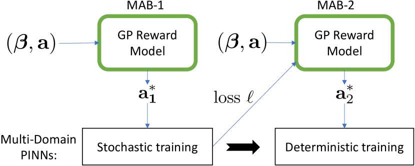
Figure 1: The illustration of the sequential MAB model.

3.2 Sequential Multi-Arm Bandits

In practice, to achieve good and reliable performance, the training of PINNs is often divided into two stages (Lu et al., 2021). The first phase is stochastic training, typically with ADAM optimizer (Kingma and Ba, 2014), to find a nice valley of the loss landscape. The second phase is deterministic optimization, typically with L-BFGS, to ensure convergence to the (local) minimum. Due to the different nature of the two phases, the ideal interface conditions can vary as well. To enable more flexible choices so as to further improve the performance, we propose a sequential MAB model, as illustrated in Fig. 1. Specifically, for each training phase, we introduce a MAB similar to Sec 3.1, which updates a separate GP reward model. To coordinate the two MAB’s and to optimize the final accuracy, the reward of the first MAB, denoted by $r_{1}$, includes not only the negative solution error after the stochastic training phase, but also a discounted error after the second phase,

$$r_{1}=-\xi_{1}+\gamma\cdot(-\xi_{2})$$ (9)

where $\gamma$ is the discount factor, and $\xi_{1}$ and $\xi_{2}$ are the solution errors after the stochastic and deterministic training phases, respectively. In this way, the influence of the interface conditions at the first training phase on the final solution accuracy is also integrated into the learning of the reward model. Next, we expand the context of the second MAB with the training loss value $\ell$ after the first phase. In this way, the training status of the first phase is also used to determine the interface conditions for the second phase. The learning of the sequential MAB’s is summarized in Algorithm 2.

Algorithm Complexity. The time complexity of both MAB algorithms is ${\mathcal{O}}(TR+\sum_{t=1}^{T}t^{3})$ where $T$ is the total number of iterations, $R$ is the complexity of multi-domain PINNs, and ${\mathcal{O}}(\sum_{t=1}^{T}t^{3})$ is the total time complexity of updating the GP reward model to $T$. In practice, $T$ is typically chosen as a few hundreds (see the experimental section). Under such a choice, running multi-domain PINNs is much more costly than GP training, and the complexity is dominant by ${\mathcal{O}}(TR)$. Hence, the time complexity is linear in the number of iterations. The space complexity of our algorithm is ${\mathcal{O}}(C+T^{2})$, including the storage of the GP reward model and the multi-domain PINN (with constant complexity ${\mathcal{O}}(C)$).

Algorithm 1 METALIC-single($T$)

1:  Initialize the GP reward model, and $\mathcal{D}\leftarrow\emptyset$.

2:  for $t=1\ldots T$ do

3:     Randomly sample the PDE parameters $\bm{\beta}\in{\mathcal{X}}$.

4:     For each action ${\bf a}\in{\mathcal{P}}$, compute the predictive distribution of the GP reward model, $\mathcal{N}\left(\mu({\bf a},\bm{\beta}),\sigma^{2}({\bf a},\bm{\beta})\right)$.

5:     Compute the UCB score: $\text{UCB}({\bf a})=\mu+\sqrt{c_{t}}\cdot\sigma$ or TS score: $\text{TS}({\bf a})\sim\mathcal{N}(\mu,\sigma^{2})$.

6:     ${\bf a}^{*}=\operatornamewithlimits{argmax}_{{\bf a}\in{\mathcal{P}}}\text{UCB}({\bf a})$ or ${\bf a}^{*}=\operatornamewithlimits{argmax}_{{\bf a}\in{\mathcal{P}}}\text{TS}({\bf a})$.

7:     Use the interface conditions of ${\bf a}^{*}$ to train the multi-domain PINNs to solve the PDE parameterized by $\bm{\beta}$, and evaluate the solution error $\xi$.

8:     $\mathcal{D}\leftarrow\mathcal{D}\cup\{\left([{\bf a}^{*},\bm{\beta}],-\xi\right)\}$.

9:     Retrain the GP reward model on $\mathcal{D}$.

10:  end for

Algorithm 2 METALIC-seq($\gamma$, $T$)

1:  Initialize two GP reward models. Set their training sets $\mathcal{D}_{1}$ and $\mathcal{D}_{2}$ to empty.

2:  repeat

3:     Randomly sample $\bm{\beta}\in{\mathcal{X}}$.

4:     Based on the predictive distribution of the first GP model, use UCB or TS to select the best action ${\bf a}^{*}_{1}$.

5:     Use the interface conditions of ${\bf a}^{*}_{1}$ to train the multi-domain PINNs with ADAM. Evaluate the error $\xi_{1}$ for solving the PDE parameterized by $\bm{\beta}$.

6:     Given the current training loss $\ell$ and $\bm{\beta}$, compute the predictive distribution of the second GP reward model for each action, and use UCB or TS to select the best action ${\bf a}^{*}_{2}$.

7:     Use the interface conditions of ${\bf a}^{*}_{2}$ to continue the training with L-BFGS. Evaluate the solution error $\xi_{2}$.

8:     $\mathcal{D}_{1}\leftarrow\mathcal{D}_{1}\cup\{\left([{\bf a}^{*}_{1},\bm{\beta}],-\xi_{1}-\gamma\xi_{2}\right)\},\mathcal{D}_{2}\leftarrow\mathcal{D}_{2}\cup\{([{\bf a}^{*}_{2},\bm{\beta},\ell],-\xi_{2})\}$.

9:     Retrain the two GP models on $\mathcal{D}_{1}$ and $\mathcal{D}_{2}$, respectively.

10:  until $T$ iterations are done

4 Related Work

As an alternative to mesh-based numerical methods, PINNs have had many success stories, e.g., (Raissi et al., 2020; Chen et al., 2020; Sirignano and Spiliopoulos, 2018; Zhu et al., 2019; Geneva and Zabaras, 2020; Sahli Costabal et al., 2020). Multi-domain PINNs, e.g., XPINNs (Jagtap and Karniadakis, 2021) and cPINNs (Jagtap et al., 2020), extend PINNs based on domain decomposition and use a set of PINNs to solve the PDE in different subdomains. To stitch together the subdomains, XPINNs used solution continuity and residual continuity as the interface conditions. Other conditions are also available, such as the flux conservation in cPINNs (Jagtap et al., 2020), the gradient continuity (De Ryck et al., 2022), and the residual gradient continuity in gPINNs (Yu et al., 2022). Recently, Hu et al. (2021) developed a theoretical understanding on the convergence and generalization properties of XPINNs, and examined the trade-off between XPINNs and PINNs.

Meta learning (Schmidhuber, 1987; Naik and Mammone, 1992; Thrun and Pratt, 2012) is an important topic in machine learning. The existing works can be roughly attributed to three categories: (1) metric-learning that learns a metric space with which the tasks can make predictions via matching the training points, e.g., nonparametric nearest neighbors (Koch et al., 2015; Vinyals et al., 2016; Snell et al., 2017; Oreshkin et al., 2018; Allen et al., 2019), (2) learning black-box models (e.g., neural networks) that map the task dataset and hyperparameters to the optimal model parameters or parameter updating rules, e.g., (Andrychowicz et al., 2016; Ravi and Larochelle, 2017; Santoro et al., 2016; Wang et al., 2016; Munkhdalai and Yu, 2017; Mishra et al., 2017), and (3) bi-level optimization where the outer level optimizes the hyperparameters and the inner level optimizes the model parameters given the hyperparameters (Finn et al., 2017; Finn, 2018; Bertinetto et al., 2018; Lee et al., 2019; Zintgraf et al., 2019; Li et al., 2017; Zhou et al., 2018). The bi-level optimization approaches are often restricted by the high cost of computing the meta-gradient (e.g., w.r.t the model initialization) via computational graphs. The issue has been recently addressed by (Li et al., 2023) that uses gradient flows to model the inner-optimization and adjoint state methods to compute the meta-gradients. Recently, Penwarden et al. (2023) developed the first method to meta learn the initialization for PINNs.

Multi-arm bandit is a classical online decision making framework (Lai et al., 1985; Auer et al., 2002a, b; Mahajan and Teneketzis, 2008; Bubeck et al., 2012), and have numerous applications, such as online advertising (Avadhanula et al., 2021), collaborative filtering (Li et al., 2016), clinical trials (Aziz et al., 2021) and robot control (Laskey et al., 2015). To our knowledge, our work is the first to use MAB for meta learning of task-specific hyperparameters, which is advantageous in its simplicity and efficiency. MAB can be viewed as an instance of reinforcement learning (RL) (Sutton and Barto, 2018), but it only needs to estimate a reward function online. While one can design more expressive RL models to meanwhile learn a Markov decision process (in MAB, we simply use UCB or TS), it often demands we run a massive number of PINN training trajectories, which is much more expensive. The model estimation is also much more challenging.

5 Experiment

To evaluate METALIC, we considered four benchmark equation families. We list the equations and domain decomposition settings in the following.

The Poisson Equation. First, we considered a 2D Poisson equation with a parameterized source function,

$$u_{xx}+u_{yy}=\widetilde{f}(x,y;s)$$ (10)

where $(x,y)\in[0,1]\times[0,1]$, $\widetilde{f}(x,y;s)=f(x,y;s)/\max_{x,y}f(x,y;s)$, and

$$f(x,y;s)=\left[\text{erf}((x-0.25)s)-\text{erf}((x-0.75)s)\right]$$

$$\cdot\left[\text{erf}((y-0.25)s)-\text{erf}((y-0.75)s)\right],$$ (11)

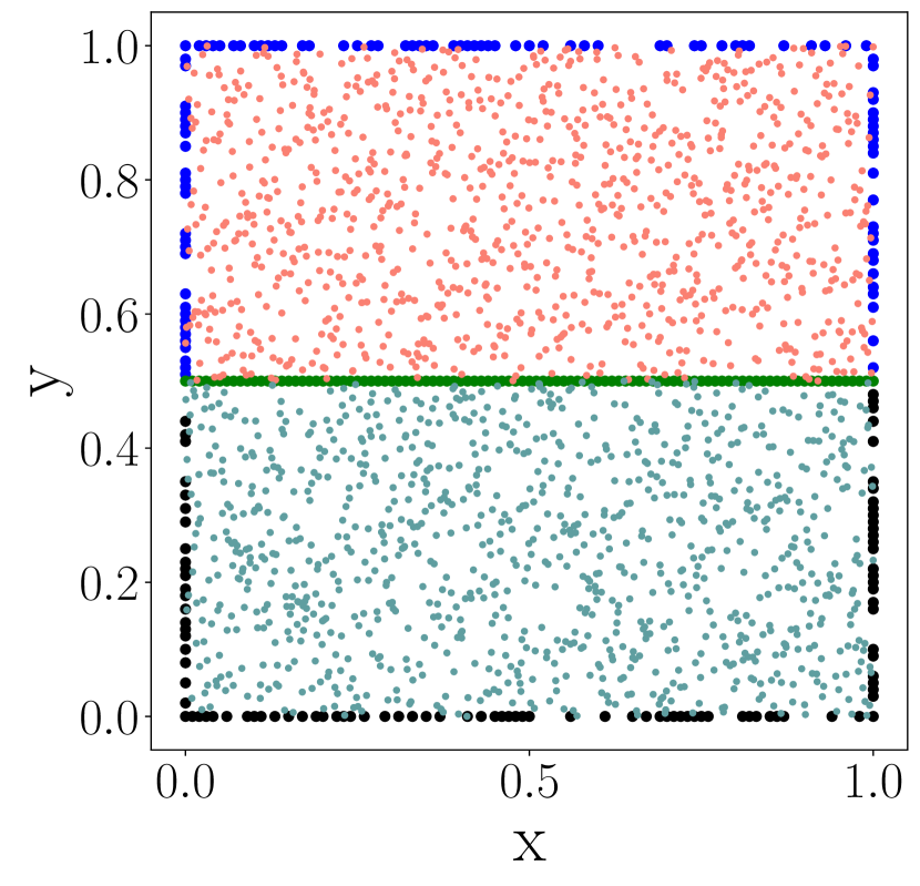
(b) Subdomains

Figure 9: The Poisson equation. The interface is the green line at $y=0.5$. Blue and black dots show the sampled boundary points in each subdomain, and the internal dots (red and cyan) are the sampled collocation points inside each subdomain.

where $\text{erf}(z)=\frac{2}{\sqrt{\pi}}\int_{0}^{z}e^{-t^{2}}{\rm d}t$, and $s\in[0,50]$ is called the sharpness parameter that controls the sharpness of the interior square in the source. We used Dirichlet boundary conditions, and ran a finite difference solver to obtain an accurate “gold-standard” solution. To run multi-domain PINNs, we split the domain into two subdomains, where the interface is a line at $y=0.5$. We visualize an exemplar solution and the subdomains, including the sampled boundary and collocation points in Fig. 9.

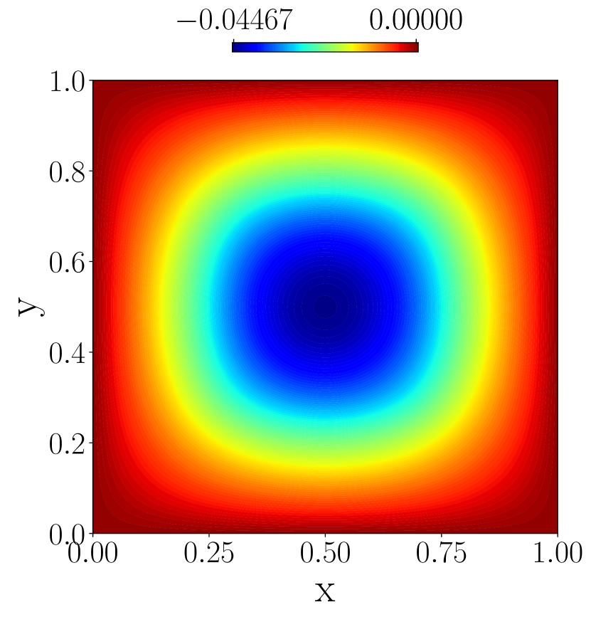
(a) Solution at $s=20$

(b) Subdomains

Figure 2: The Poisson equation. The interface is the green line at $y=0.5$. Blue and black dots show the sampled boundary points in each subdomain, and the internal dots (red and cyan) are the sampled collocation points inside each subdomain.

Advection Equation. We next considered a 1D advection (one-way wave) equation,

$$u_{t}+\beta u_{x}=0$$

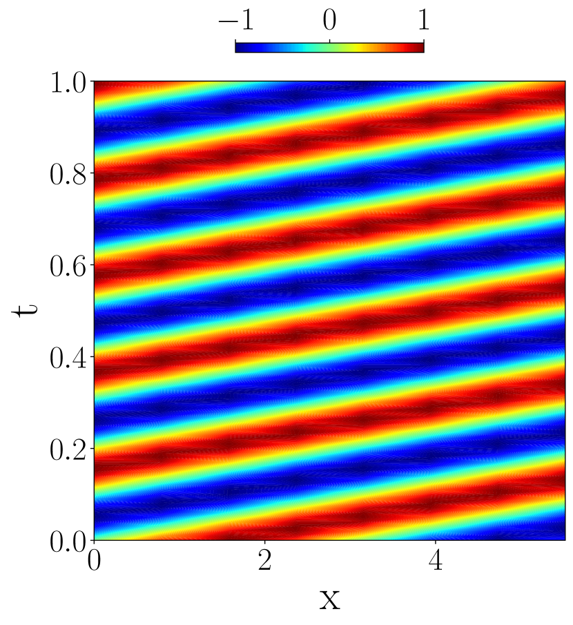
(a) Solution at $\beta=30$

(b) Subdomains

Figure 10: Advection equation. The interface is the green line at $t=0.5$.

where $x\in[0,2\pi]$, $t\in[0,1]$, and $\beta$ is the PDE parameter denoting the wave speed. We used Dirichlet boundary conditions, and the solution has an analytical form, $u(x,t)=h(x-\beta t)$ were $h(x)$ is the initial condition (which we select as $h(x)=\sin(x)$). For domain decomposition, we split the domain at $t=0.5$ to obtain two subdomains. Fig. 10 shows an exemplar solution and the subdomains with the interface.

(a) Solution at $\beta=30$

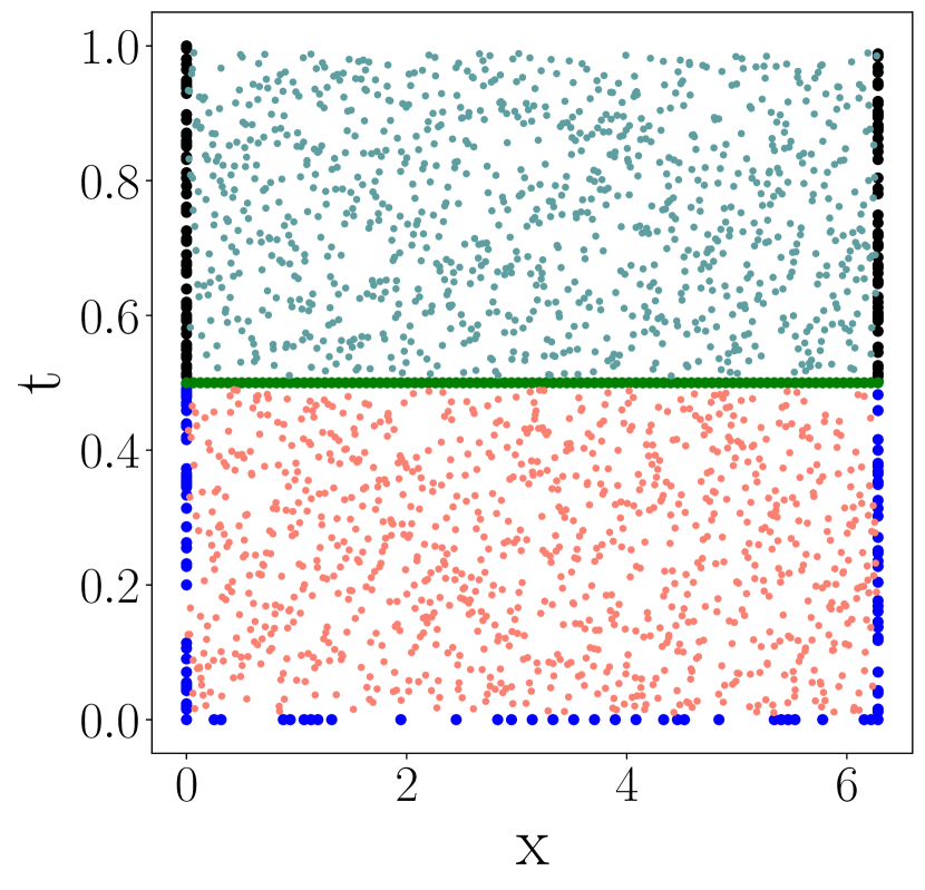
(b) Subdomains

Figure 3: Advection equation. The interface is the green line at $t=0.5$.

Reaction Equation. Third, we evaluate a 1D reaction equation,

$$u_{t}-\rho u(1-u)=0$$

where $\rho$ is the reaction coefficient (ODE parameter), $x\in[0,2\pi]$, $t\in[0,1]$ and $u(x,0)=e^{-\frac{(x-\pi)^{2}}{2(\pi/4)^{2}}}$. The exact solution is $u(x,t)=u(x,0)\cdot[e^{\rho t}/\left(u(x,0)e^{\rho t}+1-u(x,0)\right)]$. We split the domain at $t=0.5$ to obtain two subdomains. Although not required for well-posedness of the ODE system, because we are solving for the PINN space-time field $u(x,t)$, we use the exact solution to define a boundary loss term. This enhances training without compromising the time partitioning we wish to highlight. We show a solution example and the subdomains in Fig. 11.

Burger’s Equation. Fourth, we considered the viscous Burger’s equation,

$$u_{t}+uu_{x}=\nu u_{xx}$$

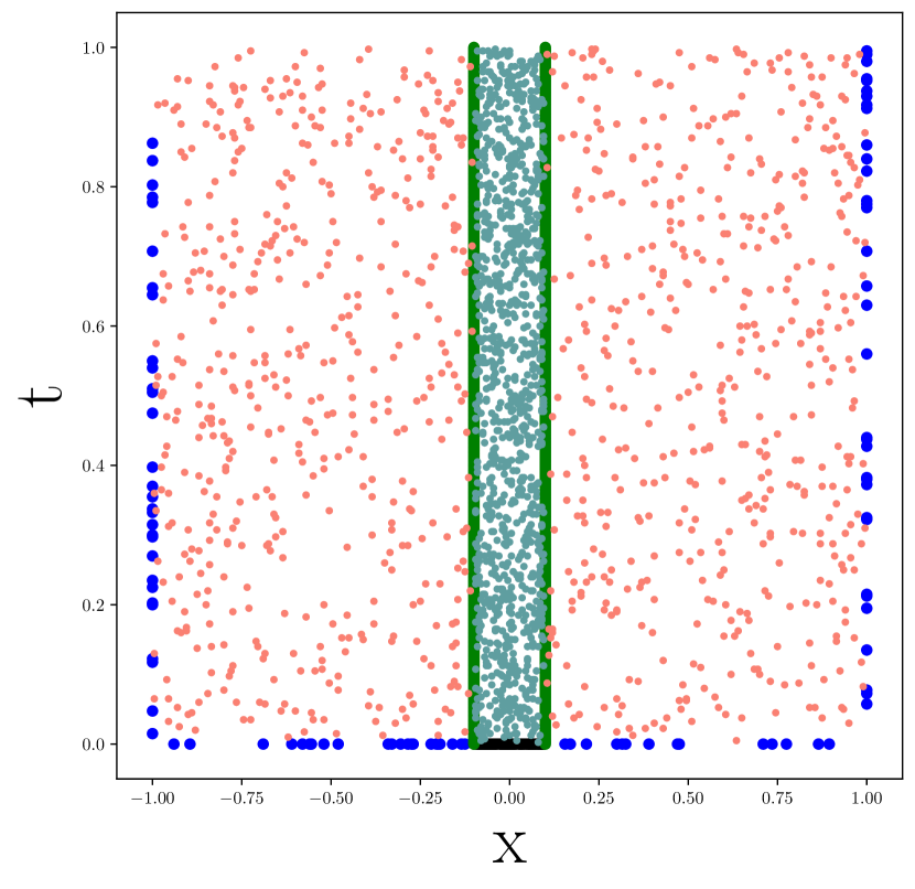
(b) Subdomains

Figure 12: Burger’s equation. The interfaces are at $x=-0.1$ and $x=0.1$. The middle portion (filled with cyan dots) is the first subdomain, and the remaining parts constitute the second subdomain.

where $\nu\in[0.001,0.05]$ is the viscosity (PDE parameter), $x\in[-1,1]$, $t\in[0,1]$, and $u(x,0)=-\sin(\pi x)$. We ran a numerical solver to obtain an accurate “gold-standard” solution. To decompose the domain, we take the middle portion that includes the shock waves as one subdomain, namely, $\Omega_{1}:x\in[-0.1,0.1],t\in[0,1]$, and the remaining as the other subdomain, $\Omega_{2}:x\in[-1,-0.1]\cap[0.1,1],t\in[0,1]$. Hence, the interface consists of two lines. See Fig. 12 for the illustration and solution example.

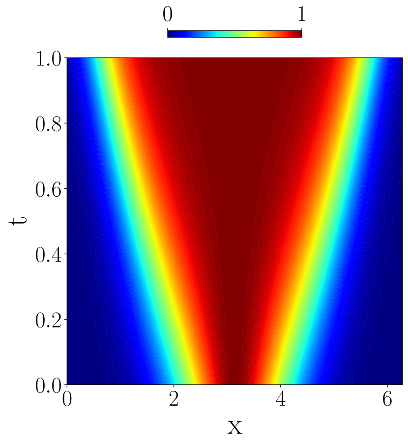
(a) Solution at $\rho=5.0$

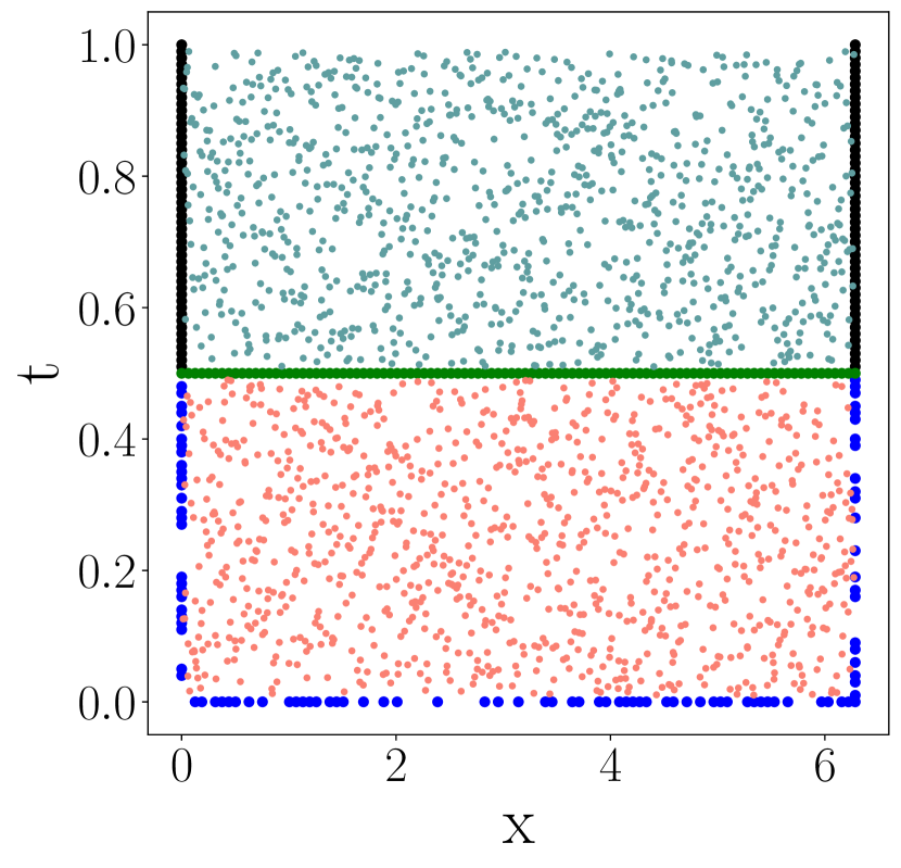
(b) Subdomains

Figure 4: Reaction equation. The interface is at $t=0.5$.

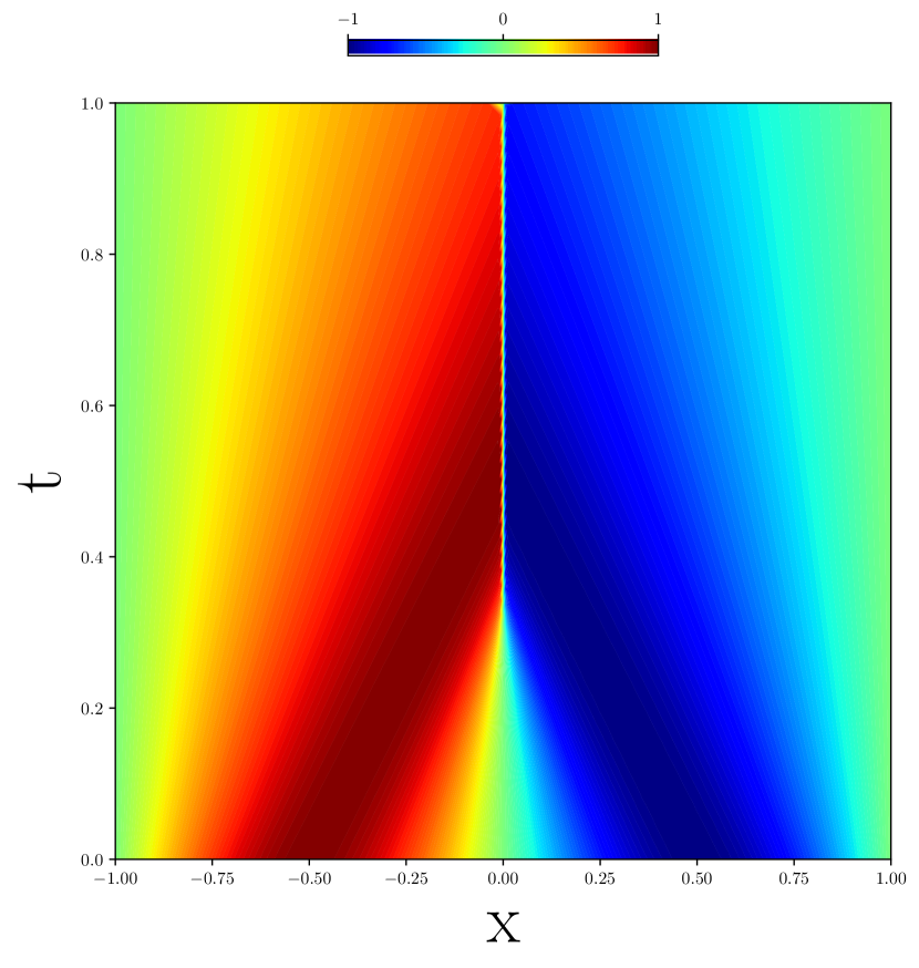
(a) Solution at $\nu=0.001$

(b) Subdomains

Figure 5: Burger’s equation. The interfaces are at $x=-0.1$ and $x=0.1$. The middle portion (filled with cyan dots) is the first subdomain, and the remaining parts constitute the second subdomain.

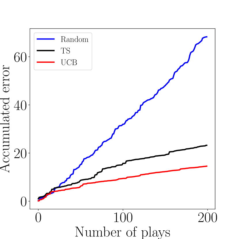
(a) Poisson equation

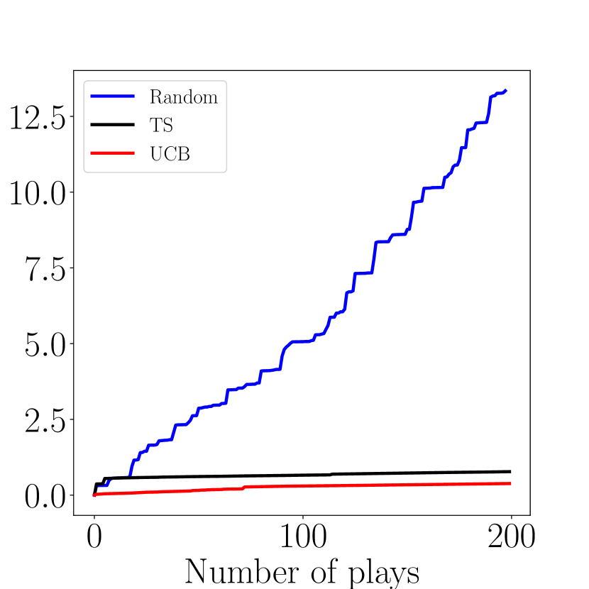
(b) Advection equation

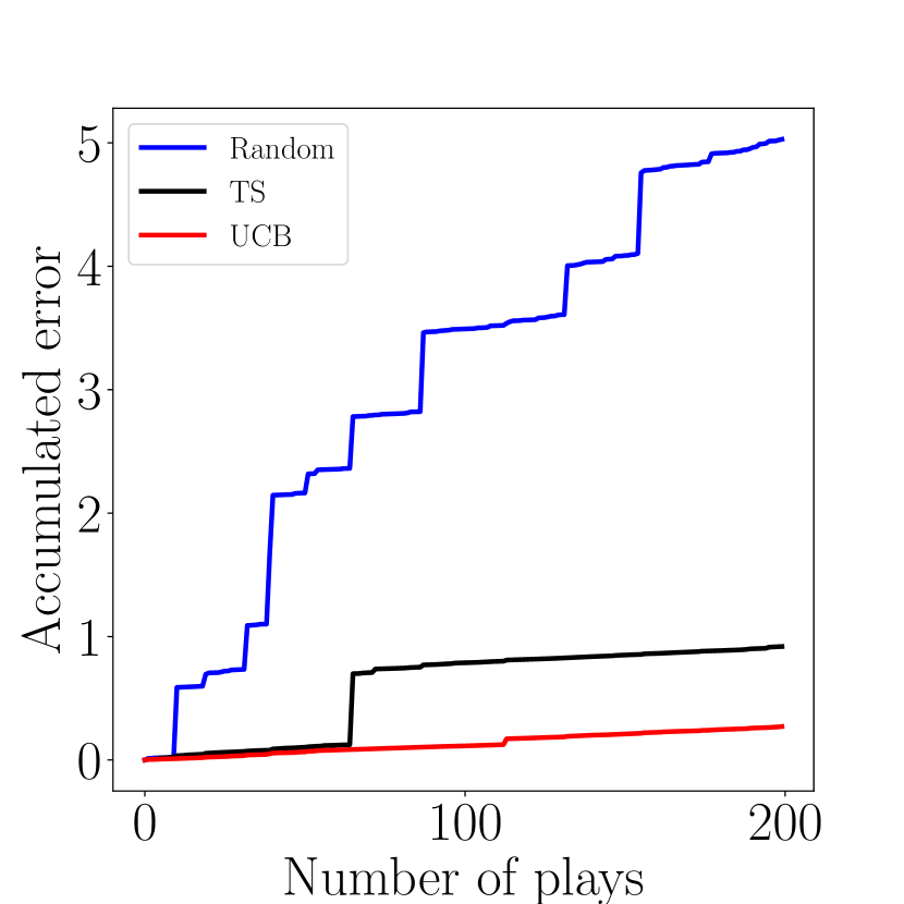
(c) Reaction equation

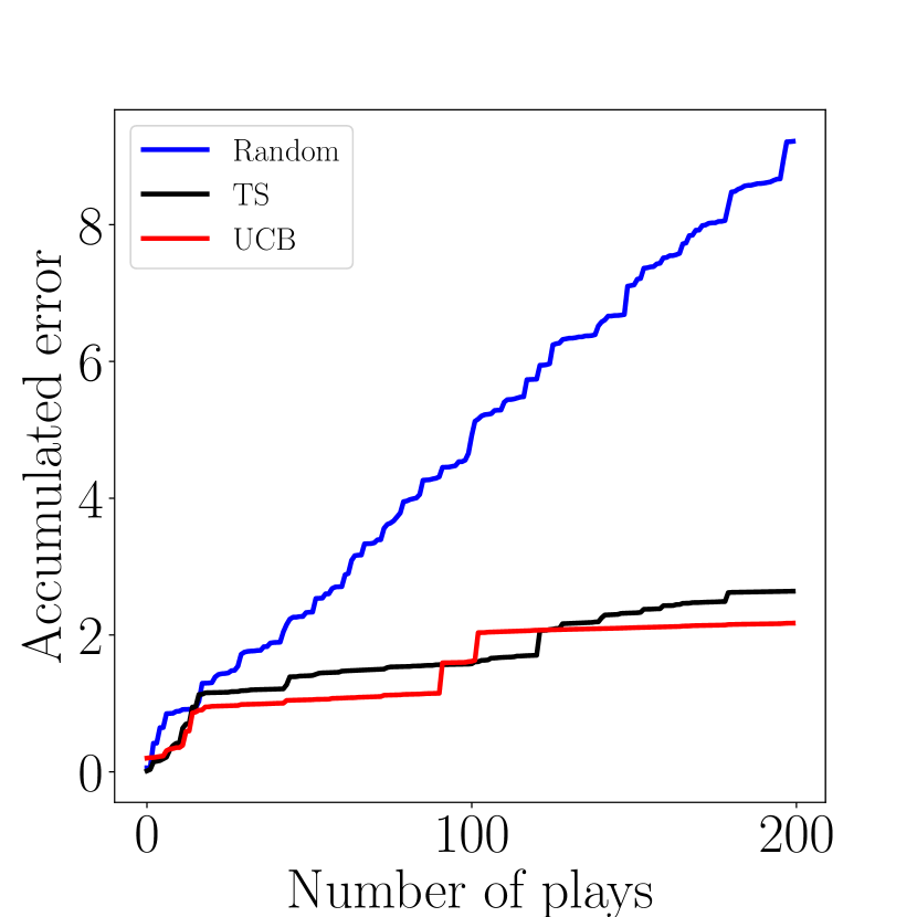
(d) Burgers’ equation

Figure 6: Online performance of METALIC-single.

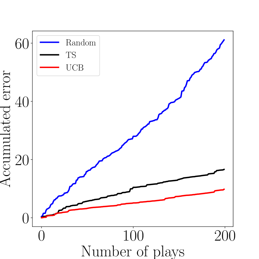
(a) Poisson equation

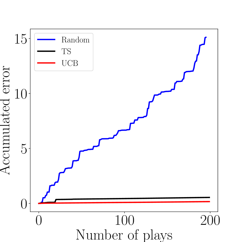
(b) Advection equation

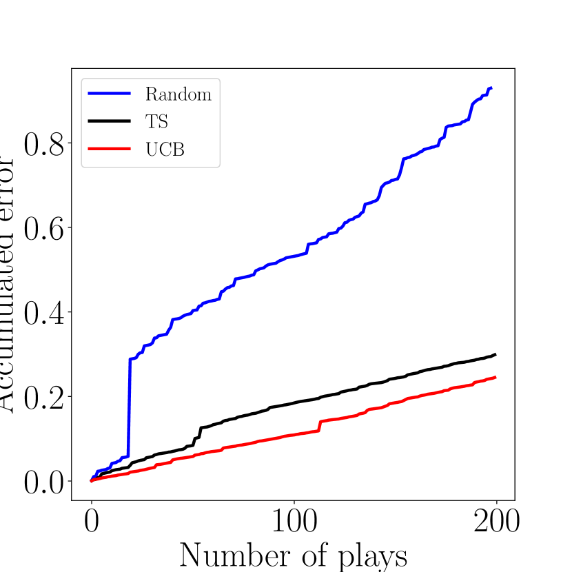
(c) Reaction equation

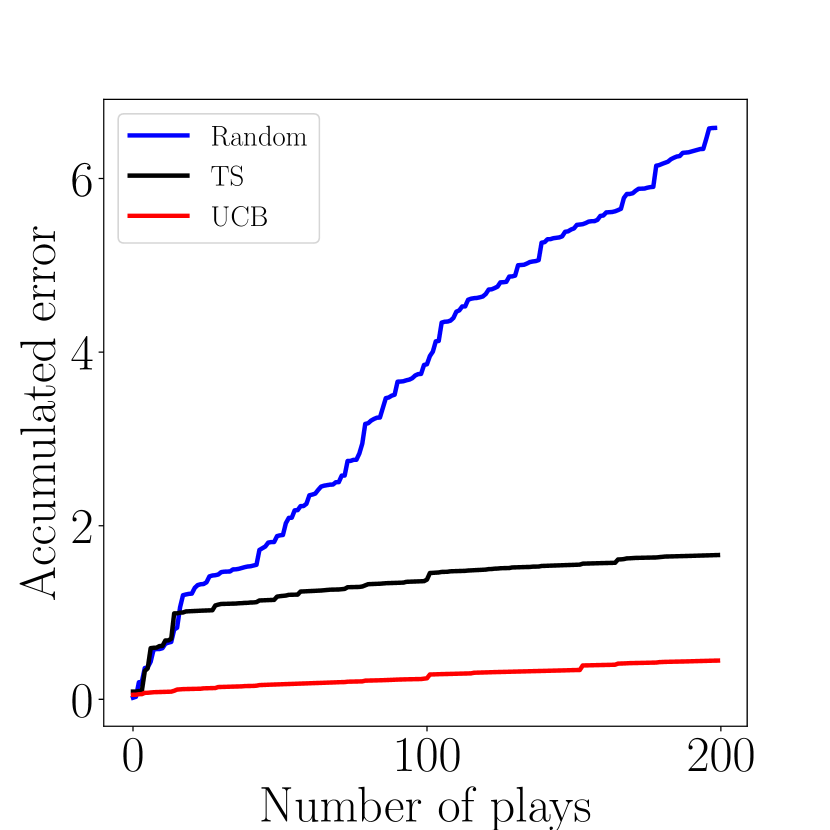
(d) Burgers’ equation

Figure 7: Online performance of METALIC-seq.

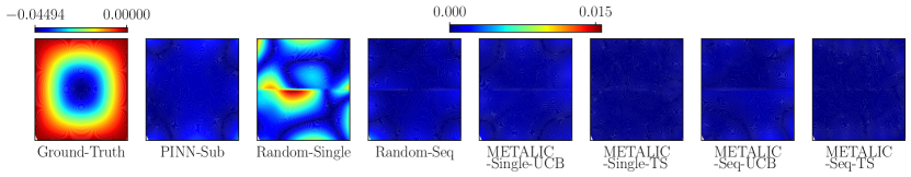
(a) Poisson equation ($s=46.1$)

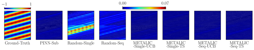
(b) Advection equation ($\beta=24.02$)

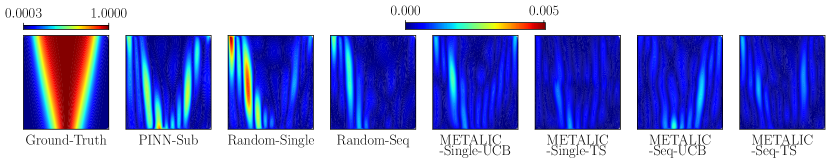
(c) Reaction equation ($\rho=4.1$)

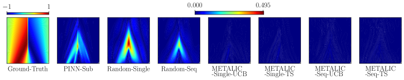
(d) Burgers’ equation ($\nu=0.0036$)

Figure 8: Point-wise solution error.

To evaluate METALIC, we used 9 interface conditions, which are listed in the supplementary material. For the PINN in each subdomain, we used two layers, with 20 neurons per layer and tanh activation function. We randomly sampled 1,000 collocation points and 100 boundary points for each PINN. To inject the interface conditions, we then randomly sampled 101 interface points for the Poisson, advection and reaction equations, and 802 interface points for Burger’s equation. We set $\lambda_{b}=20$ and $\lambda_{I}=5$, which follows the insight of (Wang et al., 2021, 2022) to adopt large weights for the boundary and interface terms so as to prevent the training of PINNs from being dominated by the residual term. We denote our single MAB by METALIC-single, and sequential MABs by METALIC-seq. For the latter, we set the discount factor $\gamma=0.9$ (see (9)). For better numerical stability, we used the relative $L_{2}$ error in the log domain to obtain the reward for updating the GP surrogate models. The running of the multi-domain PINNs consists of 10K ADAM epochs (with learning rate $10^{-3}$) and then 50K L-BFGS iterations (the first order optimality and parameter change tolerances set to $10^{-6}$ and $10^{-9}$ respectively). We set $c=1$ to compute the UCB score. We ran 200 plays (trials) for our method. For static (offline) test, we randomly sampled 100 PDEs (which do not overlap with the PDEs sampled during the online playing). We then used the learned reward model to determine the best interface conditions for each particular PDE (according to the predictive mean), with which we ran the multi-domain PINNs to solve the PDE, and computed the relative $L_{2}$ error.

Method	Poisson	Advection	Reaction	Burger’s
Random-Single	0.3992 $\pm$ 0.0037	0.07042 $\pm$ 0.01575	0.00612 $\pm$ 0.000278	0.04021 $\pm$ 0.00057
Random-Seq	0.3004 $\pm$ 0.0032	0.03922 $\pm$ 0.00919	0.01284$\pm$ 0.000707	0.03486 $\pm$ 0.00066
PINN-Sub	0.03078 $\pm$ 0.00177	0.00130 $\pm$ 8.108e-5	0.00213 $\pm$ 0.00021	0.00738 $\pm$ 0.00313
PINN-Merge-H	0.02398 $\pm$ 0.00144	0.00098 $\pm$ 5.038e-5	0.00223 $\pm$ 0.00026	0.00951 $\pm$ 0.00390
PINN-Merge-V	0.02184 $\pm$ 0.00211	0.00079 $\pm$ 3.391e-5	0.00099 $\pm$ 0.00013	0.00276 $\pm$ 0.00041
METALIC-Single-TS	0.02503 $\pm$ 0.0002	0.00079 $\pm$ 4.5897e-5	0.00204 $\pm$ 1.013e-4	0.00109 $\pm$ 1.306e-5
METALIC-Single-UCB	0.0245$\pm$ 0.0002	0.00078 $\pm$ 3.6771e-5	0.00102 $\pm$ 8.945e-6	0.00161 $\pm$ 2.939e-5
METALIC-Seq-TS	0.01639$\pm$ 9.5384e-5	0.00078 $\pm$ 3.6473e-5	0.00099 $\pm$ 8.4704e-6	0.00152 $\pm$ 5.571e-5
METALIC-Seq-UCB	0.01406 $\pm$ 9.1099e-5	0.00070 $\pm$ 3.2790e-5	0.00099 $\pm$ 5.999e-6	0.00139 $\pm$ 3.948e-5

Table 1: The average $L_{2}$ relative error of single-domain PINNs and multi-domain PINNs for solving 100 test PDEs. The interface conditions of the multi-domain PINNs are provided by METALIC and random selection. {Single, Seq} indicate using a single set or two sequential sets of interface conditions for the running of the multi-domain PINNs. {TS, UCB} corresponds to our method using TS or UCB score to determine the interface conditions at each play.

First, to examine the online performance of METALIC, we looked into the accumulated solution error along with the number of plays. We compared with randomly selecting the arm at each play. In the case of running METALIC-seq, this baseline correspondingly randomly selects the arm twice, one at the stochastic training phase, and the other at the deterministic phase. The results are shown in Fig. 6 and 7. As we can see, the accumulated error of METALIC with both UCB and TS grows much slower, i.e., sublinearly, than the random selection approach (note that the reward of the optimal action is unknown due to the randomness in the running of PINNs, and we cannot compute the regret). This has shown that our method achieves a much better exploration-exploitation tradeoff in the online interface condition decision and model updating, which is consist with many other MAB applications (see Sec 4). The results demonstrate the advantage of our MAB-based approach. First, via effective exploration, METALIC can collect valuable training examples (rewards at new actions and context) to improve the learning efficiency and performance of the GP reward surrogate model. Second, the online decision also takes advantage of the predictive abaility of the current reward model, i.e., exploitation, to select effective interface conditions, which results in increasingly better solution accuracy of the multi-domain PINNs. The online nature of METALIC enables us to keep improving the reward model while utilizing it to solve new equations with promising accuracy.

Next, we conducted an offline test, namely, without online exploration and model updates any more after 200 plays. We compared with (1) Random-Single, which, for each PDE, randomly selects a set of interface conditions applied to the entire training of the multi-domain PINNs, and (2) Random-Seq, which for each PDE, randomly selects two sets of interface conditions, one for the stochastic training and the other for the deterministic training phase. We also tested single-domain PINNs that do not incorporate interface conditions. Specifically, we compared with (3) PINN-Sub, which used the same architecture as the PINN in each subdomain, but applied to the entire domain, (4) PINN-Merge-H, which horizontally pieced all the PINNs in the subdomains, i.e., doubling the layer width yet fixing the depth, (5) PINN-Merge-V, which vertically stacked the PINNs, i.e., doubling the depth while fixing the width. Note that while PINN-Merge-H and PINN-Merge-V merge the PINNs in each subdomain, the total number of neurons actually increases (for connecting these PINNs). Hence, the merged PINN is more expressive. Each single-domain PINN used the union of the boundary points and collocation points from every subdomain. We used the same weight for the boundary term, i.e., $\lambda_{b}=20$. The running of each single-domain PINN follows exactly the same setting of the multi-domain PINNs (i.e., 10K ADAM epochs and 50K L-BFGS iterations).

We report the average relative $L_{2}$ solution error and the standard deviation in Table 1. As we can see, randomly selecting interface conditions, no matter for the whole training procedure or two training phases, result in much worse solution accuracy of multi-domain PINNs. The solution error is one order of magnitude bigger than METALIC in all the settings. It confirms that the success of the multi-domain PINNs is up to appropriate interface conditions. Next, we can observe that while the performance of METALIC-Single is similar to METALIC-Seq, the best solution accuracy is in most cases obtained by interface conditions selected by METALIC-Seq (except in solving the Burger’s equation). It demonstrates that our sequential MAB model that can employ different conditions for the two training phases is more flexible and brings additional improvement. We also observe that in most cases using the UCB for online playing can lead to better performance for both METALIC-Single and METALIC-Seq. This is consistent with the online performance evaluation (see Fig. 6 and 7). Third, among the single-domain PINN methods, PINN-Merge-V outperforms PINN-sub in all the equation families and PINN-Merge-H outperforms PINN-sub in the Poisson and advection equations, showing that deeper or wider architectures can help further improve the solution accuracy. However, their performance is still second to the best setting of METALIC, which uses simpler subdomain PINN architectures and fewer total learnable parameters. These multi-domain PINNs can be further parallelized to accelerate training. By contrast, if the interface conditions are inferior, such as those selected by Random-Single and Random-Seq, the solution error becomes much worse (orders of magnitude bigger) than single-domain PINNs. Together these results have shown the importance of the interface conditions for multi-domain PINNs and the advantage of our method.

For a fine-grained comparison, we visualize the point-wise solution error of PINN-Sub, Random-Single, Random-Seq, and our method in solving four random instances of the equations. As shown in Fig. 8, the point-wise error of both METALIC-Single and METALIC-Seq is quite uniform across the domain and close to zero (dark blue). By contrast, the competing methods often exhibit relative large errors in a few local regions, e.g., those in the middle (where the shock waves appear) of the domain of the Burger’s equation (PINN-Sub, Random-Single, Random-Seq), and the central part of the domain of the Poisson and advection equation (Random-Single). It shows that our method not only can give a superior global accuracy, but locally also better recovers individual solution values.

Finally, we analyzed the selected interface conditions in each equation family by METALIC. We found that those conditions are interesting, physically meaningful, and consistent with the properties of the equations. Due to the space limit, we provide the detailed analysis and discussion in the supplementary material.

6 Conclusion

We have presented METALIC, a simple, efficient and powerful meta learning approach to select PDE-specific interface conditions for general multi-domain PINNs. The results at four bench-mark equation families are encouraging. In the future, we will use the PDE residual as the approximate reward so that our method can be fully unsupervised. We will also extend METALIC to meta learn the interface locations along with the conditions, as a function of not only accuracy but training time so as to improve both the solution accuracy and training efficiency of the multi-domain PINNs.

Appendix

7 Interface Conditions

We used a total number of 9 interface conditions throughout all the experiments, which are listed in Table 1. Note that $I_{z}$ and $I_{zz}$ correspond to the first and second-order derivatives w.r.t an input to the PDE solution function. Since all the test PDE problems consist of two spatial or spatiotemporal dimensions, $I_{z}$ and $I_{zz}$ give four interface conditions. There are no mixed derivatives across different input dimensions. In the case that one $I_{z}$ is the same as $I_{c}$, such as in Poisson equation, the de-duplication gives 9 different conditions. In the case that all $I_{z}$’s are different from $I_{c}$, such as in Burger’s equation, we used $I_{c}$ and removed one $I_{z}$ ($z=y$ or $z=t$), so that we still maintain 9 interface conditions to be consistent with other experiments.

Table 2: Interface Conditions of Multi-domain PINNs

$I_{u}$	Solution continuity (12)
$I_{u_{avg}}$	Average solution continuity (13)
$I_{r}$	Residual (14)
$I_{rc}$	Residual continuity (15)
$I_{gr}$	Gradient-enhanced residual (16)
$I_{c}$	Flux continuity (17)
$I_{z}$	First-order spatial/temporal derivative continuity (18)
$I_{zz}$	Second-order spatial/temporal derivative continuity (19)

$$I_{u}(\bm{\theta}_{k},\bm{\theta}_{k^{\prime}})=\frac{1}{J_{k,k^{\prime}}}\sum_{i=1}^{J_{k,k^{\prime}}}\left({\widehat{u}}_{\bm{\theta}_{k}}({\bf x}_{k,k^{\prime}}^{i})-{\widehat{u}}_{\bm{\theta}_{k^{\prime}}}({\bf x}_{k,k^{\prime}}^{i})\right)^{2}$$ (12)

$$I_{u_{avg}}(\bm{\theta}_{k},\bm{\theta}_{k^{\prime}})=\frac{1}{J_{k,k^{\prime}}}\sum_{i=1}^{J_{k,k^{\prime}}}\left({\widehat{u}}_{\bm{\theta}_{k}}({\bf x}_{k,k^{\prime}}^{i})-{\widehat{u}}^{\text{avg}}_{k,k^{\prime}}({\bf x}_{k,k^{\prime}}^{i})\right)^{2}$$ (13)

$$\text{where}\;{\widehat{u}}^{\text{avg}}_{k,k^{\prime}}({\bf x}_{k,k^{\prime}}^{i})=\frac{1}{2}\left({\widehat{u}}_{\bm{\theta}_{k}}({\bf x}_{k,k^{\prime}}^{i})+{\widehat{u}}_{\bm{\theta}_{k^{\prime}}}({\bf x}_{k,k^{\prime}}^{i})\right)$$

$$I_{r}(\bm{\theta}_{k},\bm{\theta}_{k^{\prime}})=\frac{1}{J_{k,k^{\prime}}}\sum_{i=1}^{J_{k,k^{\prime}}}\left(\left({\mathcal{F}}[{\widehat{u}}_{\bm{\theta}_{k}}]({\bf x}_{k,k^{\prime}}^{i})-f({\bf x}_{k,k^{\prime}}^{i})\right)^{2}+\left({\mathcal{F}}[{\widehat{u}}_{\bm{\theta}_{k^{\prime}}}]({\bf x}_{k,k^{\prime}}^{i})-f({\bf x}_{k,k^{\prime}}^{i})\right)^{2}\right)$$ (14)

$$I_{rc}(\bm{\theta}_{k},\bm{\theta}_{k^{\prime}})=\frac{1}{J_{k,k^{\prime}}}\sum_{i=1}^{J_{k,k^{\prime}}}\left(\left({\mathcal{F}}[{\widehat{u}}_{\bm{\theta}_{k}}]({\bf x}_{k,k^{\prime}}^{i})-f({\bf x}_{k,k^{\prime}}^{i})\right)-\left({\mathcal{F}}[{\widehat{u}}_{\bm{\theta}_{k^{\prime}}}]({\bf x}_{k,k^{\prime}}^{i})-f({\bf x}_{k,k^{\prime}}^{i})\right)\right)^{2}$$ (15)

$$I_{gr}(\bm{\theta}_{k},\bm{\theta}_{k^{\prime}})=\frac{1}{J_{k,k^{\prime}}}\sum_{i=1}^{J_{k,k^{\prime}}}\sum_{j=1}^{2}\left(\left|\frac{\partial}{\partial{\bf x}_{k,k^{\prime}}^{i}[j]}\left({\mathcal{F}}[{\widehat{u}}_{\bm{\theta}_{k}}]({\bf x}_{k,k^{\prime}}^{i})-f({\bf x}_{k,k^{\prime}}^{i})\right)\right|^{2}+\left|\frac{\partial}{\partial{\bf x}_{k,k^{\prime}}^{i}[j]}\left({\mathcal{F}}[{\widehat{u}}_{\bm{\theta}_{k^{\prime}}}]({\bf x}_{k,k^{\prime}}^{i})-f({\bf x}_{k,k^{\prime}}^{i})\right)\right|^{2}\right)$$ (16)

$$I_{c}(\bm{\theta}_{k},\bm{\theta}_{k^{\prime}})=\frac{1}{J_{k,k^{\prime}}}\sum_{i=1}^{J_{k,k^{\prime}}}\left(\phi\left({\widehat{u}}_{\bm{\theta}_{k}}({\bf x}_{k,k^{\prime}}^{i})\right)\cdot{\bf n}-\phi\left({\widehat{u}}_{\bm{\theta}_{k^{\prime}}}({\bf x}_{k,k^{\prime}}^{i})\right)\cdot{\bf n}\right)^{2}$$ (17)

$$\text{where}\;\phi({\widehat{u}}_{\bm{\theta}})\cdot{\bf n}\;\text{are fluxes normal at the interface}$$

$$I_{z}(\bm{\theta}_{k},\bm{\theta}_{k^{\prime}})=\frac{1}{J_{k,k^{\prime}}}\sum_{i=1}^{J_{k,k^{\prime}}}\left(\frac{\partial}{\partial z^{i}}{\widehat{u}}_{\bm{\theta}_{k}}({\bf x}_{k,k^{\prime}}^{i})-\frac{\partial}{\partial z^{i}}{\widehat{u}}_{\bm{\theta}_{k^{\prime}}}({\bf x}_{k,k^{\prime}}^{i})\right)^{2}$$ (18)

$$\text{where}\;z^{i}={\bf x}^{i}_{k,k^{\prime}}[1]\;\text{or}\;z^{i}={\bf x}^{i}_{k,k^{\prime}}[2].$$

$$I_{zz}(\bm{\theta}_{k},\bm{\theta}_{k^{\prime}})=\frac{1}{J_{k,k^{\prime}}}\sum_{i=1}^{J_{k,k^{\prime}}}\left(\frac{\partial^{2}}{\partial{z^{i}}^{2}}{\widehat{u}}_{\bm{\theta}_{k}}({\bf x}_{k,k^{\prime}}^{i})-\frac{\partial^{2}}{\partial{z^{i}}^{2}}{\widehat{u}}_{\bm{\theta}_{k^{\prime}}}({\bf x}_{k,k^{\prime}}^{i})\right)^{2}$$ (19)

$$\text{where}\;z^{i}={\bf x}^{i}_{k,k^{\prime}}[1]\;\text{or}\;z^{i}={\bf x}^{i}_{k,k^{\prime}}[2].$$

(a) Solution at $s=20$

(a) Solution at $\rho=5.0$

(b) Subdomains

Figure 11: Reaction equation. The interface is at $t=0.5$.

(a) Solution at $\nu=0.001$

8 Regret Bound Proof

Recall that $\mathcal{X}\subseteq\mathbb{R}^{d}$ is a compact set denoting the parameter (context) space associated with the parametrized PDE, and $\mathcal{S}$ is the state space consisting of a finite number of interface conditions, i.e. $|\mathcal{S}|=s\in\mathbb{N}$. The action space $\mathcal{P}$ is defined as

$$\mathcal{P}=2^{\mathcal{S}}=\{(q_{1},\cdots,q_{s})\in\{0,1\}^{s}\}\subset\mathbb{R}^{s}.$$

In our paper, the reward at time $t$ is modeled as

$$r_{t}=r(\bm{\beta}_{t},a_{t})=f(\bm{\beta}_{t},a_{t})+\eta_{t} (\bm{\beta}_{t},a_{t})\in\mathcal{X}\times\mathcal{P},$$ (20)

where $\bm{\beta}_{t}$ is the context revealed at time $t$, $a_{t}$ is the selected action, $f$ is a function on $\mathcal{X}\times\mathcal{P}$ sampled from an appropriate prior, and $\eta_{t}$ is a white noise process used to model the extraneous randomness (e.g. neural network implementation, error rounding, etc.)

In our case, the true reward is the negative error metric computed for the learned PDE solution, which is too complicated for analysis. Alternatively, we use the above model (20) as a substitute for approximation. As a result, the reward model is misspecified. Nevertheless, we assume that (20) is reflective of the true reward and do not consider the model misspecification effects in the subsequent analysis for ease of demonstration; ideas from (Bogunovic and Krause, 2021) can be used to obtain refined analysis for misspecified models but we do not pursue them here.

We now state the technical assumptions on the model parametrization as used in the METALIC algorithm:

• $f(\bm{\beta},a)$ is sampled from a $\mathcal{GP}(0,\kappa)$ prior, where $\kappa$ is a kernel function on $\mathcal{X}\times\mathcal{P}\subset\mathbb{R}^{d+s}$:

  $$\kappa((\bm{\beta},a),(\bm{\beta}^{\prime},a^{\prime}))=\kappa_{1}(\bm{\beta},\bm{\beta}^{\prime})\kappa_{2}(a,a^{\prime}),$$

  where $\kappa_{1}$ and $\kappa_{2}$ are Gaussian kernels:

  $$\kappa_{1}(\bm{\beta},\bm{\beta}^{\prime})=\exp(-\tau_{1}\|\bm{\beta}-\bm{\beta}^{\prime}\|_{2}^{2}) \kappa_{2}(a,a^{\prime})=\exp\left(-\frac{\tau_{2}}{s}\|a-a^{\prime}\|_{1}\right).$$

  (Note: The key assumption we will be using the is the tensor product structure as well as the form of $\kappa_{1}$; since $\kappa_{2}$ is discrete, it does not encode much of geometry and changing to other alternatives should not affect the subsequent analysis. )

• $\eta_{t}$ are i.i.d. Gaussian with variance $\sigma_{0}^{2}$:

  $$\eta_{t}\stackrel{{\scriptstyle\text{i.i.d.}}}{{\sim}}N(0,\sigma_{0}^{2}).$$

Under the above assumptions, for $T\in\mathbb{N}$ and historical observations ${\bf x}_{t}=(\bm{\beta}_{t},a_{t})\in\mathcal{X}\times\mathcal{P}$, $1\leq t\leq T$, $y_{T}=(r_{1},\cdots,r_{T})^{\top}$, the posterior distribution of $f$ at ${\bf x}=(\bm{\beta},a)\in\mathbb{R}^{d+s}$ is a normal random variable with mean and variance given below:

$$\mu_{T}({\bf x}) =k^{\top}_{T}({\bf x})(\sigma_{0}^{2}I_{T}+K_{T})^{-1}y_{T}$$

$$\sigma_{T}^{2}({\bf x}) =\kappa({\bf x},{\bf x})-k^{\top}_{T}({\bf x})(\sigma_{0}^{2}I_{T}+K_{T})^{-1}k_{T}({\bf x}),$$

where

$$K_{T}=(\kappa({\bf x}_{i},{\bf x}_{j}))_{1\leq i,j\leq T}\in\mathbb{R}^{T\times T} k_{T}({\bf x})=(\kappa({\bf x},{\bf x}_{1}),\cdots,\kappa({\bf x},{\bf x}_{T}))^{\top}\in\mathbb{R}^{T}.$$

The following quantity, which measures the maximum uncertainty reduction of $f_{T}=(f({\bf x}_{1}),\cdots,f({\bf x}_{T}))^{\top}$ when observing $y_{T}$, will appear in the regret analysis:

$$\gamma_{T} :=\max_{\{{\bf x}_{t}\}\subset\mathcal{X}\times\mathcal{P}}H(f_{T})-H(f_{T}|y_{T})$$

$$=\max_{\{{\bf x}_{t}\}\subset\mathcal{X}\times\mathcal{P}}H(y_{T})-H(y_{T}|f_{T})\ \ \ \ \ \ \ \ \text{$H(y_{T}|f_{T})$ is independent of $\{{\bf x}_{t}\}$}$$

$$=\max_{\{{\bf x}_{t}\}\subset\mathcal{X}\times\mathcal{P}}\frac{1}{2}\log|I_{T}+\sigma_{0}^{-2}K_{T}|,$$

where $H$ is the Shannon entropy.

We are now ready to state the main result:

Theorem 8.1

For $\delta>0$, take $c_{t}$ in the UCB algorithm as

$$c_{t}=2\log\left(\frac{2^{s}\pi^{2}t^{2}}{6\delta}\right) t\in\mathbb{N}.$$

Conditioning on every context sequence $\{\bm{\beta}_{t}\}$, let $\{a_{t}\}$ be the action selected by the UCB algorithm under the above choice of $\{c_{t}\}$. Then, with probability at least $1-\delta$, the regret $R_{T}$ satisfies

$$R_{T}\lesssim\sqrt{\frac{2^{s}T(\log T)^{d+1}\log\left(\frac{2^{s}T^{2}}{\delta}\right)}{\log(1+\sigma_{0}^{-2})}} T=1,2,\cdots,$$ (21)

where the implicit constant is absolute (does not depend on $\{\bm{\beta}_{t}\}$ but depends on the domain $\mathcal{X}$). In particular,

$$\mathbb{E}[R_{T}]\lesssim\sqrt{\frac{2^{s}T(\log T)^{d+1}\log\left(2^{s}T^{2}\right)}{\log(1+\sigma_{0}^{-2})}},$$ (22)

Moreover, (22) holds also for the Thompson sampling algorithm.

Proof  We first prove the statement concerning the UCB algorithm. The proof is similar to (Krause and Ong, 2011) overall. Owing to a few subtle differences, we provide a sketch of the proof. In our setting, contexts are revealed in a random fashion that is independent of the reward noises. For convenience, we condition on the context sequence $\{\bm{\beta}_{t}\}_{t\in\mathbb{N}}\subset\mathcal{X}$ throughout the analysis, i.e., we treat $\{\bm{\beta}_{t}\}_{t\in\mathbb{N}}\subset\mathcal{X}$ as deterministic and arbitrary sequence.

Firstly, a standard application of concentration inequalities and a union bound (Krause and Ong, 2011, supplement, Lemma 5.2) yields that, with probability at least $1-\delta$,

$$|f(\bm{\beta}_{t},a)-\mu_{t}(\bm{\beta}_{t},a)|\leq c_{t}^{1/2}\sigma_{t-1}(\bm{\beta}_{t},a) t\in\mathbb{N},\ a\in\mathcal{P},$$ (23)

which immediately implies an upper bound for the regret:

$$R_{T} =\sum_{t=1}^{T}(f(\bm{\beta}_{t},a_{t}^{*})-f(\bm{\beta}_{t},a_{t}))\ \ \ \ \ \ \ \ \ a_{t}^{*}=\arg\max_{a\in\mathcal{P}}f(\bm{\beta}_{t},a)$$

$$\leq\sum_{t=1}^{T}\underbrace{(\mu_{t-1}(\bm{\beta}_{t},a_{t}^{*})+c_{t}^{1/2}\sigma_{t-1}(\bm{\beta}_{t},a_{t}^{*}))-(\mu_{t-1}(\bm{\beta}_{t},a_{t})+c_{t}^{1/2}\sigma_{t-1}(\bm{\beta}_{t},a_{t}))}_{\leq 0}+2c_{t}^{1/2}\sigma_{t-1}(\bm{\beta}_{t},a_{t})$$

$$\leq 2\sum_{t=1}^{T}c_{t}^{1/2}\sigma_{t-1}(\bm{\beta}_{t},a_{t})$$

$$\leq 2\sqrt{T}\left[c_{T}\sum_{t=1}^{T}\sigma^{2}_{t-1}(\bm{\beta}_{t},a_{t})\right]^{1/2}\ \ \ \ \ \ \ \text{(Cauchy--Schwarz; $c_{t}$ is increasing in $t$)}$$

$$\stackrel{{\scriptstyle(\star)}}{{\leq}}\sqrt{\frac{8Tc_{T}\gamma_{T}}{\log(1+\sigma_{0}^{-2})}}$$

$$\lesssim K(\sigma_{0})\sqrt{Tc_{T}\gamma_{T}}\ \ \ \ \ \ \ \ \ \ \ \ \ K(\sigma_{0})=\sqrt{\frac{1}{\log(1+\sigma_{0}^{-2})}},$$

where the ($\star$) follows from (Krause and Ong, 2011, Theorem 5) and an intuitive way to understand it is that the total information gain (i.e. the predictive variance term; see (Srinivas et al., 2009, Lemma 5.3)) is bounded by the maximum information gain under the optimal design.

It remains to bound $\gamma_{T}$ for the kernel $\kappa$. Since $\kappa$ is a tensor product of $\kappa_{1}$ and $\kappa_{2}$, with $\kappa_{2}$ being a kernel on a discrete set with cardinality $2^{s}$ (i.e. has rank $2^{s}$), according to (Krause and Ong, 2011, Theorem 2),

$$\gamma_{T}\leq 2^{s}(\gamma_{T}|_{\kappa_{1}}+\log T),$$

where $\gamma_{T}|_{\kappa_{1}}$ is the maximum information gain defined for the GP with kernel function $\kappa_{1}$. Note $\kappa_{1}$ is the Gaussian kernel. (Srinivas et al., 2009, Theorem 5) tells us that $\gamma_{T}|_{\kappa_{1}}=\mathcal{O}((\log T)^{d+1})$, where the implicit constant depends on the domain $\mathcal{X}$. Hence, $\gamma_{T}\lesssim 2^{s}(\log T)^{d+1}$. Plugging this into the above bound for $R_{T}$ yields the high-probability bound (21). For (22), note that (21) and $\sqrt{x+y}\leq\sqrt{x}+\sqrt{y},x,y\geq 0$ together imply that there exists an absolute constant $C>0$ so that with probability at least $1-\delta$,

$$\widetilde{R}_{T}:=\frac{\left|R_{T}-CK(\sigma_{0})\sqrt{2^{s}T(\log T)^{d+1}\log\left(2^{s}T^{2}\right)}\right|}{CK(\sigma_{0})\sqrt{2^{s}T(\log T)^{d+1}}}\leq\sqrt{\log\left(\frac{1}{\delta}\right)},$$

i.e., ${\bf P}(\widetilde{R}_{T}\geq x|\{\bm{\beta}_{t}\})\leq e^{-x^{2}}$. Integrating the tail probability yields

$$\mathbb{E}[\widetilde{R}_{T}|\{\bm{\beta}_{t}\}]=\int_{0}^{\infty}{\bf P}(\widetilde{R}_{T}\geq x|\{\bm{\beta}_{t}\})dx\leq\int_{0}^{\infty}e^{-x^{2}}dx=\sqrt{\pi}.$$

Taking expectation over $\{\bm{\beta}_{t}\}$ yields $\mathbb{E}[\widetilde{R}_{T}]\leq\sqrt{\pi}$. (22) follows by rearrangement.

For $a_{t}$ chosen according to the Thompson sampling, we employ a similar technique that appears in (Lattimore and Szepesvári, 2020, Theorem 36.1). First, note that for any two random variables $Z_{t},Z^{\prime}_{t}$ with the same mean,

$$\mathbb{E}[f(\bm{\beta}_{t},a_{t}^{*})-f(\bm{\beta}_{t},a_{t})]=\mathbb{E}[f(\bm{\beta}_{t},a_{t}^{*})-Z_{t}+Z_{t}^{\prime}-f(\bm{\beta}_{t},a_{t})].$$

Conditioning on the historical actions $\{a_{s}\}_{1\leq s\leq t-1}$ and rewards $\{r_{s}\}_{1\leq s\leq t-1}$ up to $t-1$ (i.e. the $\sigma$-field $\mathcal{F}_{t-1}$), $a_{t}$ and $a_{t}^{*}$ are the argmax of $f(\bm{\beta}_{t},a)$ and $f^{\prime}(\bm{\beta}_{t},a)$, respectively, where $f(\bm{\beta}_{t},a)$ and $f^{\prime}(\bm{\beta}_{t},a)$ have the same distribution (i.e. posterior distribution of $f$). As a result, $a_{t}$ and $a_{t}^{*}$ have the same $\mathcal{F}_{t-1}$-conditional distribution. Now take $Z_{t}$ and $Z_{t}^{\prime}$ as the UCB scores of $a_{t}^{*}$ and $a_{t}$ at $t-1$, respectively:

$$Z_{t}=\mu_{t-1}(\bm{\beta}_{t},a_{t}^{*})+c_{t}^{1/2}\sigma_{t-1}(\bm{\beta}_{t},a^{*}_{t}) Z^{\prime}_{t}=\mu_{t-1}(\bm{\beta}_{t},a_{t})+c_{t}^{1/2}\sigma_{t-1}(\bm{\beta}_{t},a_{t}).$$

It is easy to verify using the tower property that $\mathbb{E}[Z_{t}]=\mathbb{E}[\mathbb{E}[Z_{t}|\mathcal{F}_{t-1}]]=\mathbb{E}[\mathbb{E}[Z^{\prime}_{t}|\mathcal{F}_{t-1}]]=\mathbb{E}[Z_{t-1}]$. On the other hand, according to (23), it holds with probability at least $1-2\delta$ that

$$f(\bm{\beta}_{t},a_{t}^{*})-Z_{t}+Z_{t}^{\prime}-f(\bm{\beta}_{t},a_{t})\leq c_{t}^{1/2}\sigma_{t-1}(\bm{\beta}_{t},a) t\in\mathbb{N}.$$

Using a similar analysis in the UCB case, we conclude that

$$\mathbb{E}[R_{T}]=\sum_{t=1}^{T}\mathbb{E}[f(\bm{\beta}_{t},a_{t}^{*})-Z_{t}+Z_{t}^{\prime}-f(\bm{\beta}_{t},a_{t})]\lesssim\sqrt{\frac{2^{s}T(\log T)^{d+1}\log\left(2^{s}T^{2}\right)}{\log(1+\sigma_{0}^{-2})}}.$$

 

9 Preliminary Study of the Interface Conditions

We conducted a preliminary study on a 2D Poisson equation $u_{xx}+u_{yy}=1$ with the solution shown in Figure 13.

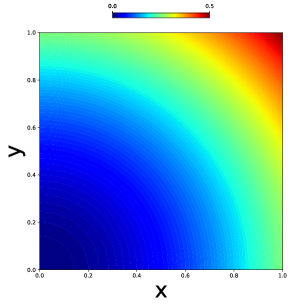
Figure 13: Poisson solution.

Given this PDE problem, we compared three types of boundary and collocation point sampling methods: random, grid, and Poisson disc sampling, as shown in Figure 14. The comparison was done between a standard PINN and XPINN, where the number of collocation points in each XPINN subdomain is the same as the total number of collocation points used by the PINN. We trained the two models with the boundary loss term weight $\lambda_{b}$ set to 1 and 20. We also varied the interface loss term weight $\lambda_{I}$ from {1, 20}. The interface loss term is computed from (13) and (15). Table 3 shows the $L_{2}$ relative error averaged over 10 runs to minimize the variance in network initialization and optimization. We can see that the XPINN performance is relevantly less variant to differences in sampling and weights, but for PINNs these differences result in order of magnitude changes in error. For this reason, we have conducted all the evaluations fairly by using random sampling and larger boundary weights for PINN’s which was the best overall setting. We also make the insight that random sampling allows a PINN to see higher frequencies according to the Nyquist-Shannon sampling theorem which may be the reason for increased performance over the other sampling methods. The XPINN includes an additional complexity of subdomains and interface conditions which may dominate the training, resulting in less variance as a function of collocation points.

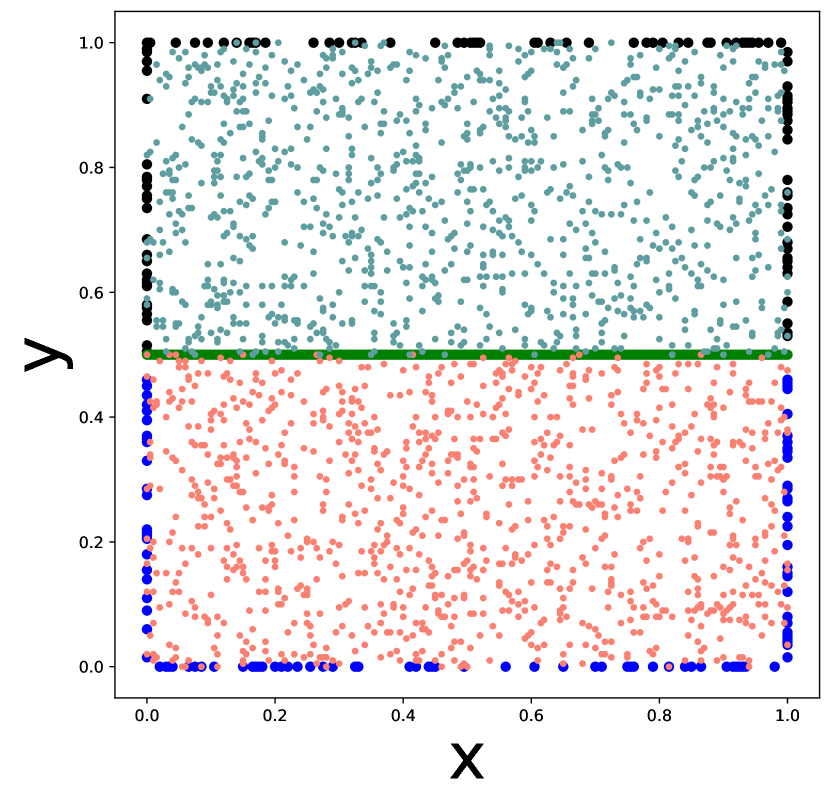
(a) Random

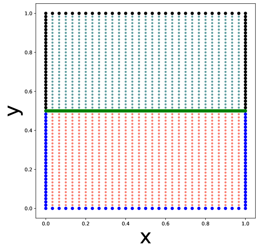
(b) Grid

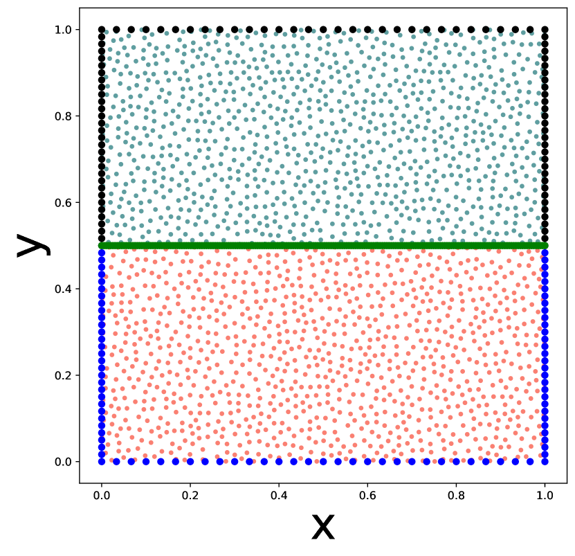
(c) Poisson Disc

Figure 14: Random, grid, and Poisson disc sampling for the Poisson equation problem. The interface is the green line at $y=0.5$. Blue and black dots show the sampled boundary points in each subdomain, and the internal dots (red and cyan) the sampled points inside each subdomain.

Model	Random		Grid		Poisson Disc
	$\lambda_{b,I}$ = 1	$\lambda_{b,I}$ = 20	$\lambda_{b,I}$ = 1	$\lambda_{b,I}$ = 20	$\lambda_{b,I}$ = 1	$\lambda_{b,I}$ = 20
PINN	9.0325e-4	4.3223e-4	6.0278e-3	2.3699e-3	5.3902e-3	2.2375e-3
XPINN	5.0884e-3	5.3205e-3	6.0764e-3	4.7829e-3	6.5061e-3	4.4888e-3

Table 3: Average $L_{2}$ relative error over 10 runs for different sampling techniques and loss term weights.

9.1 Interface Condition Combination

For the same PDE problem with random sampling, we ran multi-domain PINNs with different sets of conditions. We used the generalized interface condition notations for multi-domain PINNs as described in Table 7. For example, an XPINN can be described as $I_{u_{avg}}+I_{rc}$. The weights on all terms are unity. As seen by the results in Table 4, the multi-domain PINNs with interfaces $I_{u_{avg}}+I_{c}+I_{yy}$ outperforms other combinations as well as the PINN. We can see that with the correct interface conditions, the multi-domain PINN can greatly improve upon the standard XPINN. In fact, the additional residual continuity term, a trait of XPINNs, performs infinitesimally better than only using the average solution continuity. These results are the foundation of the METALIC method as we have shown that different combinations of conditions result in drastically different performances. We can also see that multi-domain PINNs are more general and flexible than the existing PINN decomposition models such as XPINN and cPINN. Having only used XPINNs in Table 3, one might conclude decomposing this problem is inferior to a standard PINN. However, we have shown that cPINN outperformed XPINN by an order of magnitude and that adding the additional term $I_{yy}$ improved the cPINN even further. Furthermore, naively adding all possible terms such as in the final row, does not necessarily give the best results. This leaves three options for multi-domain PINNs: manually tuning the interface conditions, running all possible permutations such as we have done here, or devise a method to learn the appropriate interfaces such as METALIC.

Model	$L_{2}$ Relative Error
PINN	1.05e-3 ± 4.38e-4
$I_{u_{avg}}$	4.28e-3 ± 2.63e-3
$I_{u_{avg}}+I_{rc}$	3.92e-3 ± 2.25e-3
$I_{u_{avg}}+I_{c}$	9.45e-4 ± 2.85e-4
$I_{u_{avg}}+I_{rc}+I_{c}$	9.77e-4 ± 3.45e-4
$I_{u_{avg}}+I_{rc}+I_{gr}$	4.57e-3 ± 3.18e-3
$I_{u_{avg}}+I_{c}+I_{yy}$	5.26e-4 ± 1.97e-4
$I_{u_{avg}}+I_{rc}+I_{gr}+I_{c}+I_{yy}$	9.34e-4 ± 3.18e-4

Table 4: Average $L_{2}$ relative error over 10 runs for different interface combinations. Note: $I_{c}=I_{y}$ for this problem.

10 Meta Learning Result Analysis

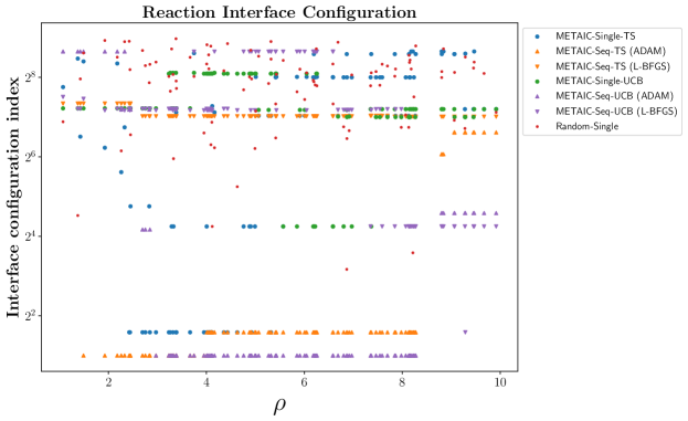
Figure 21: Scatter plot of interface configuration vs. the equation parameter $\rho$.

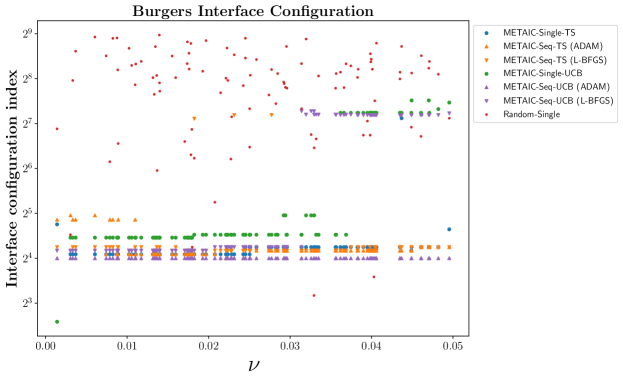
Figure 24: Scatter plot of interface configuration vs. the equation parameter $\nu$.

There are $2^{9}=512$ possible combinations of the interface conditions. For convenience, we use an integer to index each configuration (combination), $\text{index}=\sum_{i=0}^{n}2^{i}{\bf c}[i]$ where ${\bf c}$ is a list of binaries, and ${\bf c}[i]=1$ means $i$-th interface condition is turned on. We therefore can show how different sets of interface conditions are selected along with the equation parameters (see Figures 15, 18, 21, and 24).

10.1 Poisson Equation

For each PDE test case, we provide three analysis plots to better understand the METALIC results. For the Poisson problem, Figure 15 provides an overview of the interface configuration groupings as the equation parameter $s$ varies. As opposed to Random-Single, the various METALIC methods predict interface configurations in groupings based on parameter $s$. This indicates that for these ranges, the PDE solution behaves similarly across the interfaces. It can also be seen that the configurations chosen between METALIC-Single and METALIC-Seq are different, indicating that the optimization is an important factor. This is logical since at the beginning of training, the PINN must first propagate information from the initial and boundary conditions inward to the entire domain. Therefore, interface conditions during this phase may in fact make learning more difficult in terms of the loss landscape as the network is trying to enforce continuity at a location which has no information but is simply a set of random predictions given the random initialization of weights and bias of the network.

In Figure 16, we can see the number of times the interface conditions are selected over the 100 test cases. Random-Single serves as a baseline with each interface being chosen roughly half of the time. The two most noticeable trends are that the gradient-enhanced residual term is almost never chosen and the flux continuity which is equivalent to $u_{y}$ for this case is always chosen by METALIC. This is interesting as the gradient term in the original gPINN paper was shown to be beneficial to PINN training but appears to be a poor choice on a set of interface points, possibly because with all the other terms, it simply make the loss landscape more complex and does not provide a significant accuracy benefit compared to the other more theoretically sound terms such as flux. This result is novel as it showcases the robustness of METALIC in being able to distinguish between valid and invalid terms, something that would take a user doing manual tuning of these terms much trail and error to determine. We also note that the METALIC choices align with our results in Section 9.1 that the flux conditions from cPINN greatly outperforms the residual continuity conditions in XPINN for Poisson’s equation. Flux continuity is a well studied conservation term rooted in traditional methods whereas residual continuity is a term devised with the convenience of PINNs and automatic-differentiation(AD) in mind. We also note that when comparing the METALIC-Seq-UCB ADAM and L-BFGS choices, L-BFGS uses more terms on average than ADAM. This confirms our hypothesis from Figure 15 that more interface terms at the start of training may in-fact make training more difficult. This validates the result that not only is a sequential interface predictor more accurate, but also faster as it adds in terms when needed which would reduce computational cost. We also not that including the residual points in the overall set of collocation points is rarely chosen, likely due to the fact that the interface point set is an order of magnitude smaller than the collocation point set so assuming it is well sampled, its contribution is negligible. All these insights further confirm the method is working well and is consistent with our intuition and the properties of the equation being solved.

Finally, in Figure 17, we show the $L^{2}$ relative error as a function of $s$. This is a more detailed version of the error table in the manuscript which tells us how the problem difficulty changes over the parameterization of the problem. For this Poisson problem, it is quite consistent other than the lower bound around $s=1$ in which the forcing term is very smooth and as we expect the problem is quite simple, as reflected by the lower errors there.

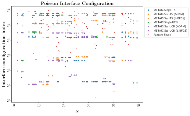
Figure 15: Scatter plot of interface configuration vs. the equation parameter $s$.

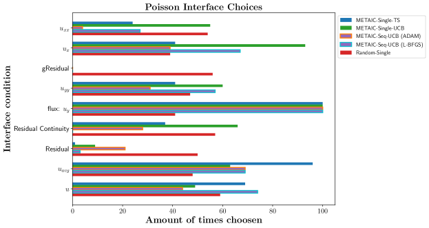
Figure 16: Horizontal bar plot of the quantity of interfaces chosen throughout testing over 100 randomly drawn equation parameters.

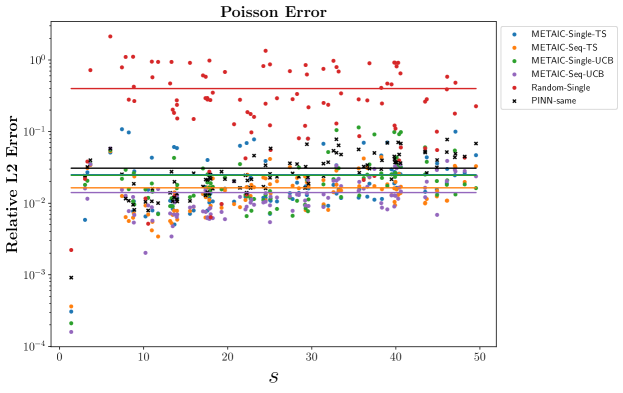
Figure 17: Scatter plot of the relative $L_{2}$ error vs. the equation parameter $s$.

10.2 Advection Equation

For the Advection problem, Figure 19 indicates that very few terms where needed. So much so that the ADAM step of METALIC-Seq-UCB has only one term, $I_{u_{avg}}$, the weaker form of the solution continuity. We again point out the benefit of METALIC in being able to sub-select few terms out of many while still resulting in the best accuracy as seen in Figures 18 & 20 which show that METALIC-Seq-UCB uses the fewest number of terms but has the best error. This emphasizes that more interface terms are not always better since the loss landscape can become more complex from an optimization standpoint. Another interesting feature is that the first derivative in space ($u_{x}$) is chosen more than the first derivative in time ($u_{t}$) despite the subdomain split being in time. This is opposite of the Poisson results in which the derivative normal to the interface ($u_{y}$), representing the flux, was chosen in all cases. Both terms, $u_{t}$ and $u_{x}$ are part of the PDE with flux simply being $u$, but the tangential derivative $u_{x}$ appears to be a much more meaningful term when it comes to propagating the wave through the interface. There are also no second order terms which was the case with Poisson.

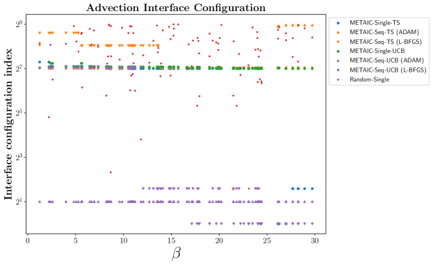
Figure 18: Scatter plot of interface configuration vs. the equation parameter $\beta$.

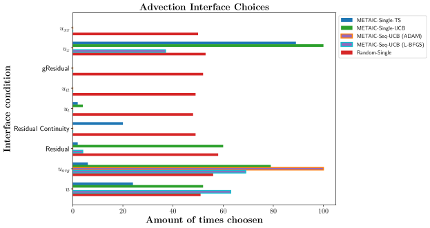
Figure 19: Horizontal bar plot of the quantity of interfaces chosen throughout testing over 100 randomly drawn equation parameters.

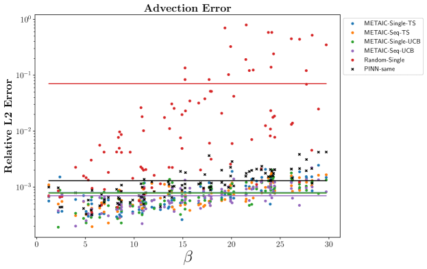
Figure 20: Scatter plot the relative $L_{2}$ error vs. the equation parameter $\beta$.

10.3 Reaction Equation

For the Reaction problem, we note that while this is an ODE, with no spatial derivatives, they were counter-intuitively chosen as interfaces. This emphasizes the fact that PINNs, and machine learning techniques in general, do not work the same as traditional methods since these terms are not necessary for well-posedness of an ODE. Given this, Figure 23 shows that METALIC outperformed the PINN while using these conditions. This is an interesting line of investigation for future work as it shows counter-intuitive terms can provide a training benefit to PINNs even in contrast to the previous Advection problem where almost no terms where chosen. It is not clear why in some cases only the most basic of terms are used while in others terms which do not make physical sense are chosen, but in both, the accuracy is quite good on their respective problems. This shows that METALIC learns something about PINN training that is not evidently clear to the human user.

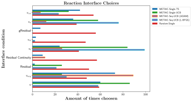
Figure 22: Horizontal bar plot of the quantity of interfaces chosen throughout testing over 100 randomly drawn equation parameters.

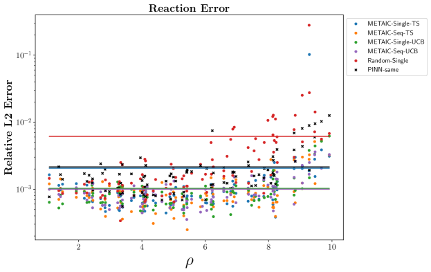
Figure 23: Scatter plot of the relative $L_{2}$ error vs. the equation parameter $\rho$.

10.4 Burger’s Equation

For the Burger’s problem, we see more of what one might expect from traditional interface continuity terms. Figure 25 shows that the flux term is predominately chosen, just as in Poisson’s equation. Although here we see the flux is not equivalent to the first order derivative, enforcing the idea that it is in fact the flux providing the training benefit and not a coincidence of the first-order derivative and flux being the same for Poisson. We also see the largest improvement in error of METALIC over PINNs as seen in Figure 26. The trend is also consistent with our physical understanding, as viscosity ($\nu$) increases the problem becomes more simple. This is because at lower viscosities a shock forms and creates a discontinuity in the solution which is difficult for PINNs to resolve. The decomposition of this problem is therefore the most sound, in that we allow one network to handle the sharp discontinuity in the center, and another to handle the relatively simple solution around it. This allows for the network in the center to learn a higher frequency basis with which to approximate the discontinuity instead of also having to fit the lower frequencies around it which has been delegated to the second network. Given this, it makes sense that a multi-domain PINN with the METALIC method greatly outperform PINNs here. It also emphasizes that in the less physically motivated decompositions for Poisson, Advection, and Reaction, we still see improvement using multi-domain PINNs and METALIC.

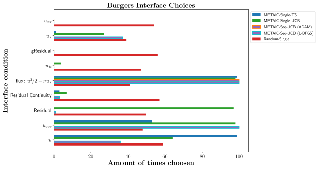
Figure 25: Horizontal bar plot of the quantity of interfaces chosen throughout testing over 100 randomly drawn equation parameters.

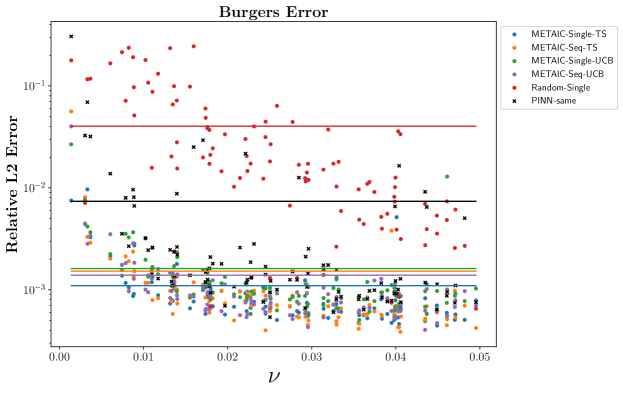
Figure 26: Scatter plot of the relative $L_{2}$ error vs. the equation parameter $\nu$.

References

- Allen et al. (2019) Kelsey Allen, Evan Shelhamer, Hanul Shin, and Joshua Tenenbaum. Infinite mixture prototypes for few-shot learning. In International Conference on Machine Learning, pages 232–241. PMLR, 2019.
- Andrychowicz et al. (2016) Marcin Andrychowicz, Misha Denil, Sergio Gomez, Matthew W Hoffman, David Pfau, Tom Schaul, Brendan Shillingford, and Nando De Freitas. Learning to learn by gradient descent by gradient descent. arXiv preprint arXiv:1606.04474, 2016.
- Auer (2002) Peter Auer. Using confidence bounds for exploitation-exploration trade-offs. Journal of Machine Learning Research, 3(Nov):397–422, 2002.
- Auer et al. (2002a) Peter Auer, Nicolo Cesa-Bianchi, and Paul Fischer. Finite-time analysis of the multiarmed bandit problem. Machine learning, 47(2):235–256, 2002a.
- Auer et al. (2002b) Peter Auer, Nicolo Cesa-Bianchi, Yoav Freund, and Robert E Schapire. The nonstochastic multiarmed bandit problem. SIAM journal on computing, 32(1):48–77, 2002b.
- Avadhanula et al. (2021) Vashist Avadhanula, Riccardo Colini Baldeschi, Stefano Leonardi, Karthik Abinav Sankararaman, and Okke Schrijvers. Stochastic bandits for multi-platform budget optimization in online advertising. In Proceedings of the Web Conference 2021, pages 2805–2817, 2021.
- Aziz et al. (2021) Maryam Aziz, Emilie Kaufmann, and Marie-Karelle Riviere. On multi-armed bandit designs for dose-finding clinical trials. Journal of Machine Learning Research, 22(1-38):4, 2021.
- Bertinetto et al. (2018) Luca Bertinetto, Joao F Henriques, Philip HS Torr, and Andrea Vedaldi. Meta-learning with differentiable closed-form solvers. arXiv preprint arXiv:1805.08136, 2018.
- Bogunovic and Krause (2021) Ilija Bogunovic and Andreas Krause. Misspecified gaussian process bandit optimization. Advances in Neural Information Processing Systems, 34:3004–3015, 2021.
- Bubeck et al. (2012) Sébastien Bubeck, Nicolo Cesa-Bianchi, et al. Regret analysis of stochastic and nonstochastic multi-armed bandit problems. Foundations and Trends® in Machine Learning, 5(1):1–122, 2012.
- Chapelle and Li (2011) Olivier Chapelle and Lihong Li. An empirical evaluation of thompson sampling. In Advances in neural information processing systems, pages 2249–2257, 2011.
- Chen et al. (2020) Yuyao Chen, Lu Lu, George Em Karniadakis, and Luca Dal Negro. Physics-informed neural networks for inverse problems in nano-optics and metamaterials. Optics express, 28(8):11618–11633, 2020.
- De Ryck et al. (2022) Tim De Ryck, Ameya D Jagtap, and Siddhartha Mishra. Error estimates for physics informed neural networks approximating the navier-stokes equations. arXiv preprint arXiv:2203.09346, 2022.
- Finn (2018) Chelsea Finn. Learning to learn with gradients. PhD thesis, UC Berkeley, 2018.
- Finn et al. (2017) Chelsea Finn, Pieter Abbeel, and Sergey Levine. Model-agnostic meta-learning for fast adaptation of deep networks. In International Conference on Machine Learning, pages 1126–1135. PMLR, 2017.
- Geneva and Zabaras (2020) Nicholas Geneva and Nicholas Zabaras. Modeling the dynamics of pde systems with physics-constrained deep auto-regressive networks. Journal of Computational Physics, 403:109056, 2020.
- Hu et al. (2021) Zheyuan Hu, Ameya D Jagtap, George Em Karniadakis, and Kenji Kawaguchi. When do extended physics-informed neural networks (xpinns) improve generalization? arXiv preprint arXiv:2109.09444, 2021.
- Jagtap and Karniadakis (2021) Ameya D Jagtap and George E Karniadakis. Extended physics-informed neural networks (xpinns): A generalized space-time domain decomposition based deep learning framework for nonlinear partial differential equations. In AAAI Spring Symposium: MLPS, 2021.
- Jagtap et al. (2020) Ameya D Jagtap, Ehsan Kharazmi, and George Em Karniadakis. Conservative physics-informed neural networks on discrete domains for conservation laws: Applications to forward and inverse problems. Computer Methods in Applied Mechanics and Engineering, 365:113028, 2020.
- Kingma and Ba (2014) Diederik P Kingma and Jimmy Ba. Adam: A method for stochastic optimization. arXiv preprint arXiv:1412.6980, 2014.
- Kissas et al. (2020) Georgios Kissas, Yibo Yang, Eileen Hwuang, Walter R Witschey, John A Detre, and Paris Perdikaris. Machine learning in cardiovascular flows modeling: Predicting arterial blood pressure from non-invasive 4d flow mri data using physics-informed neural networks. Computer Methods in Applied Mechanics and Engineering, 358:112623, 2020.
- Koch et al. (2015) Gregory Koch, Richard Zemel, and Ruslan Salakhutdinov. Siamese neural networks for one-shot image recognition. In ICML deep learning workshop, volume 2. Lille, 2015.
- Krause and Ong (2011) Andreas Krause and Cheng Ong. Contextual gaussian process bandit optimization. Advances in neural information processing systems, 24, 2011.
- Lai et al. (1985) Tze Leung Lai, Herbert Robbins, et al. Asymptotically efficient adaptive allocation rules. Advances in applied mathematics, 6(1):4–22, 1985.
- Laskey et al. (2015) Michael Laskey, Jeff Mahler, Zoe McCarthy, Florian T. Pokorny, Sachin Patil, Jur van den Berg, Danica Kragic, Pieter Abbeel, and Ken Goldberg. Multi-armed bandit models for 2d grasp planning with uncertainty. In 2015 IEEE International Conference on Automation Science and Engineering (CASE), pages 572–579, 2015. doi: 10.1109/CoASE.2015.7294140.
- Lattimore and Szepesvári (2020) Tor Lattimore and Csaba Szepesvári. Bandit algorithms. Cambridge University Press, 2020.
- Lee et al. (2019) Kwonjoon Lee, Subhransu Maji, Avinash Ravichandran, and Stefano Soatto. Meta-learning with differentiable convex optimization. In Proceedings of the IEEE/CVF Conference on Computer Vision and Pattern Recognition, pages 10657–10665, 2019.
- Li et al. (2023) Shibo Li, Zheng Wang, Akil Narayan, Robert Kirby, and Shandian Zhe. Meta-learning with adjoint methods. In International Conference on Artificial Intelligence and Statistics, pages 7239–7251. PMLR, 2023.
- Li et al. (2016) Shuai Li, Alexandros Karatzoglou, and Claudio Gentile. Collaborative filtering bandits. In Proceedings of the 39th International ACM SIGIR conference on Research and Development in Information Retrieval, pages 539–548, 2016.
- Li et al. (2017) Zhenguo Li, Fengwei Zhou, Fei Chen, and Hang Li. Meta-sgd: Learning to learn quickly for few-shot learning. arXiv preprint arXiv:1707.09835, 2017.
- Lu et al. (2021) Lu Lu, Xuhui Meng, Zhiping Mao, and George Em Karniadakis. Deepxde: A deep learning library for solving differential equations. SIAM Review, 63(1):208–228, 2021.
- Mahajan and Teneketzis (2008) Aditya Mahajan and Demosthenis Teneketzis. Multi-armed bandit problems. In Foundations and applications of sensor management, pages 121–151. Springer, 2008.
- Mishra et al. (2017) Nikhil Mishra, Mostafa Rohaninejad, Xi Chen, and Pieter Abbeel. A simple neural attentive meta-learner. arXiv preprint arXiv:1707.03141, 2017.
- Munkhdalai and Yu (2017) Tsendsuren Munkhdalai and Hong Yu. Meta networks. In International Conference on Machine Learning, pages 2554–2563. PMLR, 2017.
- Naik and Mammone (1992) Devang K Naik and Richard J Mammone. Meta-neural networks that learn by learning. In [Proceedings 1992] IJCNN International Joint Conference on Neural Networks, volume 1, pages 437–442. IEEE, 1992.
- Oreshkin et al. (2018) Boris N Oreshkin, Pau Rodriguez, and Alexandre Lacoste. Tadam: Task dependent adaptive metric for improved few-shot learning. arXiv preprint arXiv:1805.10123, 2018.
- Penwarden et al. (2023) Michael Penwarden, Shandian Zhe, Akil Narayan, and Robert M Kirby. A metalearning approach for physics-informed neural networks (PINNs): Application to parameterized PDEs. Journal of Computational Physics, page 111912, 2023.
- Raissi et al. (2019) Maziar Raissi, Paris Perdikaris, and George E Karniadakis. Physics-informed neural networks: A deep learning framework for solving forward and inverse problems involving nonlinear partial differential equations. Journal of Computational Physics, 378:686–707, 2019.
- Raissi et al. (2020) Maziar Raissi, Alireza Yazdani, and George Em Karniadakis. Hidden fluid mechanics: Learning velocity and pressure fields from flow visualizations. Science, 367(6481):1026–1030, 2020.
- Ravi and Larochelle (2017) Sachin Ravi and Hugo Larochelle. Optimization as a model for few-shot learning. In In International Conference on Learning Representations (ICLR), 2017.
- Sahli Costabal et al. (2020) Francisco Sahli Costabal, Yibo Yang, Paris Perdikaris, Daniel E Hurtado, and Ellen Kuhl. Physics-informed neural networks for cardiac activation mapping. Frontiers in Physics, 8:42, 2020.
- Santoro et al. (2016) Adam Santoro, Sergey Bartunov, Matthew Botvinick, Daan Wierstra, and Timothy Lillicrap. Meta-learning with memory-augmented neural networks. In International conference on machine learning, pages 1842–1850. PMLR, 2016.
- Schmidhuber (1987) Jürgen Schmidhuber. Evolutionary principles in self-referential learning, or on learning how to learn: the meta-meta-… hook. PhD thesis, Technische Universität München, 1987.
- Shukla et al. (2021) Khemraj Shukla, Ameya D Jagtap, and George Em Karniadakis. Parallel physics-informed neural networks via domain decomposition. Journal of Computational Physics, 447:110683, 2021.
- Sirignano and Spiliopoulos (2018) Justin Sirignano and Konstantinos Spiliopoulos. Dgm: A deep learning algorithm for solving partial differential equations. Journal of computational physics, 375:1339–1364, 2018.
- Slivkins et al. (2019) Aleksandrs Slivkins et al. Introduction to multi-armed bandits. Foundations and Trends® in Machine Learning, 12(1-2):1–286, 2019.
- Snell et al. (2017) Jake Snell, Kevin Swersky, and Richard Zemel. Prototypical networks for few-shot learning. Advances in neural information processing systems, 30, 2017.
- Srinivas et al. (2009) Niranjan Srinivas, Andreas Krause, Sham M Kakade, and Matthias Seeger. Gaussian process optimization in the bandit setting: No regret and experimental design. arXiv preprint arXiv:0912.3995, 2009.
- Srinivas et al. (2010) Niranjan Srinivas, Andreas Krause, Sham Kakade, and Matthias Seeger. Gaussian process optimization in the bandit setting: no regret and experimental design. In Proceedings of the 27th International Conference on International Conference on Machine Learning, pages 1015–1022, 2010.
- Sun et al. (2020) Luning Sun, Han Gao, Shaowu Pan, and Jian-Xun Wang. Surrogate modeling for fluid flows based on physics-constrained deep learning without simulation data. Computer Methods in Applied Mechanics and Engineering, 361:112732, 2020.
- Sutton and Barto (2018) Richard S Sutton and Andrew G Barto. Reinforcement learning: An introduction. MIT press, 2018.
- Thompson (1933) William R Thompson. On the likelihood that one unknown probability exceeds another in view of the evidence of two samples. Biometrika, 25(3/4):285–294, 1933.
- Thrun and Pratt (2012) Sebastian Thrun and Lorien Pratt. Learning to learn. Springer Science & Business Media, 2012.
- Vinyals et al. (2016) Oriol Vinyals, Charles Blundell, Timothy Lillicrap, Koray Kavukcuoglu, and Daan Wierstra. Matching networks for one shot learning. arXiv preprint arXiv:1606.04080, 2016.
- Wang et al. (2016) Jane X Wang, Zeb Kurth-Nelson, Dhruva Tirumala, Hubert Soyer, Joel Z Leibo, Remi Munos, Charles Blundell, Dharshan Kumaran, and Matt Botvinick. Learning to reinforcement learn. arXiv preprint arXiv:1611.05763, 2016.
- Wang et al. (2021) Sifan Wang, Yujun Teng, and Paris Perdikaris. Understanding and mitigating gradient flow pathologies in physics-informed neural networks. SIAM Journal on Scientific Computing, 43(5):A3055–A3081, 2021.
- Wang et al. (2022) Sifan Wang, Xinling Yu, and Paris Perdikaris. When and why pinns fail to train: A neural tangent kernel perspective. Journal of Computational Physics, 449:110768, 2022.
- Yu et al. (2022) Jeremy Yu, Lu Lu, Xuhui Meng, and George Em Karniadakis. Gradient-enhanced physics-informed neural networks for forward and inverse pde problems. Computer Methods in Applied Mechanics and Engineering, 393:114823, 2022.
- Zhou et al. (2018) Fengwei Zhou, Bin Wu, and Zhenguo Li. Deep meta-learning: Learning to learn in the concept space. arXiv preprint arXiv:1802.03596, 2018.
- Zhu et al. (2019) Yinhao Zhu, Nicholas Zabaras, Phaedon-Stelios Koutsourelakis, and Paris Perdikaris. Physics-constrained deep learning for high-dimensional surrogate modeling and uncertainty quantification without labeled data. Journal of Computational Physics, 394:56–81, 2019.
- Zintgraf et al. (2019) Luisa Zintgraf, Kyriacos Shiarli, Vitaly Kurin, Katja Hofmann, and Shimon Whiteson. Fast context adaptation via meta-learning. In International Conference on Machine Learning, pages 7693–7702. PMLR, 2019.