NON-SIMPLE POLYOMINOES OF KŐNIG TYPE and their canonical module

Abstract.

We study the Kőnig type property for non-simple polyominoes. We prove that, for closed path polyominoes, the polyomino ideals are of Kőnig type, extending the results of Herzog and Hibi for simple thin polyominoes. As an application of this result, we give a combinatorial interpretation for the canonical module of the coordinate ring of a sub-class of closed path polyominoes, namely circle closed path polyominoes. In this case, we compute also the Cohen-Macaulay type and we show that $K[\mathcal{P}]$ is a level ring.

1. Introduction

Polyominoes are plane figures obtained by joining unitary squares along their edges. They raise many combinatorial problems, for instance, tiling a certain region or the plane with polyominoes and related problems are of interest to mathematicians and computer scientists. Even though problems like, for example, the enumeration of pentominoes, have their origins in antiquity, polyominoes were formally defined by Golomb first in 1953 and later, in 1996, in his monograph [18].
The study of polyominoes reveals many connections to different subjects. For instance, in algebraic languages: there seems to be a nice relation between polyominoes and Dyck words and Motzkin words [13], statistical physics: polyominoes (and their higher-dimensional analogs known in the literature as lattice animals) appear as models of branched polymers and of percolation clusters [42].
A classic topic in commutative algebra is the study of determinantal ideals. These are the ideals generated by the $t$-minors of any matrix, and special attention is received in the case of the minors of a generic matrix, whose entries are indeterminates, see for instance [2] and [39]. More generally, ideals of $t$-minors of 2-sided ladders were studied, see [10], [11], [12], [19]. When considering the case of 2-minors, these classes of ideals are special cases of the ideal $I_{\mathcal{P}}$ of inner 2-minors of a polyomino $\mathcal{P}$ in the polynomial ring over a field $K$ in the variables $x_{v}$ where $v$ is a vertex of $\mathcal{P}$. This type of ideal called polyomino ideal, was introduced in 2012 by Qureshi [31]. Since then, the study of the main algebraic properties of a polyomino ideal and of its quotient ring $K[\mathcal{P}]=S/I_{\mathcal{P}}$ in terms of the shape of $\mathcal{P}$ has become an exciting area of research. For instance, several mathematicians have studied the primality of $I_{\mathcal{P}}$, see [3], [6], [7], [25], [26], [28], [29], [36]. Moreover, in [23] and [33], the authors showed that $K[\mathcal{P}]$ is a normal Cohen-Macaulay domain if $\mathcal{P}$ is a simple polyomino, i.e. a polyomino without holes; a precise definition will be given in Section 2. See also the references [15], [16], [17], [27], [34], [24].
Not many properties are known for non-simple polyominoes. However, the reader may consult [36] and [37], and, for the special class of closed path polyominoes, several interesting results can be found in [3], [5], [7] and [8]. In the paper [22], the authors introduced graded ideals of Kőnig type with respect to a monomial order $<$, i.e ideals $I$ for which there exists a sequence of the height of $I$ homogeneous polynomials forming part of a minimal system of generators of the ideal such that there exists a monomial order $<$ with respect to whom their initial monomials form a regular sequence. The authors presented interesting consequences that may occur when working with a graded ideal with this property. Moreover, in the paper [21], Herzog and Hibi showed that if $\mathcal{P}$ is a simple thin polyomino, then its polyomino ideal has the Kőnig type property. We are interested in understanding the Kőnig type property for non-simple polyominoes, following the path initiated by Herzog and Hibi. We will focus on a specific class of non-simple thin polyominoes, namely closed path polyominoes.
Not all polyomino ideals are of Kőnig type and there is no known classification of the polyominoes that have this property. In particular, parallelogram polyominoes give a class of simple polyominoes for which this property does not hold. Indeed, this follows by [32, Proposition 2.3], where the authors showed that parallelogram polyominoes are simple planar distributive lattices, and by using the classification of distributive lattices of Kőnig type provided in [21, Theorem 4.1]. In addition, we also found an example of a non-simple thin polyomino that cannot be of Kőnig type, see Example 4.1.
The paper is organized as follows. In Section 2, we present a detailed introduction to polyominoes and polyomino ideals, and in Lemma 2.1 we prove that, if $\mathcal{P}$ is a closed path polyomino, then its number of vertices is twice the number of its cells, a fact that will be useful in the next sections.
In order to study closed path polyominoes of Kőnig type, a combinatorial formula to compute height $I_{\mathcal{P}}$ is needed. Section 3 is devoted to this scope. In Theorem 3.4, we give a combinatorial formula for the Krull dimension of $K[\mathcal{P}]$ and prove it using the simplicial complexes theory. The fact that $\mathcal{P}$ contains some specific configurations as shown in [3, Section 6] plays a crucial role in our proof. Consequently, in Corollary 3.5, we prove that the height of $I_{\mathcal{P}}$ is the number of cells of the closed path polyomino. We conjecture that this formula holds for any non-simple polyomino.
Section 4 is devoted to the proof of the Kőnig type property of $I_{\mathcal{P}}$ for any closed path polyomino, see Theorem 4.9. In Definition 4.3, we define a suitable order on the vertices of the closed path polyomino $\mathcal{P}$ for whom the desired property holds. There are two cases to be examined: either $\mathcal{P}$ contains a configuration of four cells (treated in Proposition 4.4) or $\mathcal{P}$ has an $L$-configuration in every change of direction (treated in Proposition 4.7). In addition, we present concrete examples to illustrate our procedures.
The canonical module of coordinate rings of polyominoes has never been studied. Just recently, in the article [35], the authors have studied the levelness property for a special class of simple thin polyominoes. In Section 5, we study the canonical module of the coordinate ring for a sub-class of closed path polyominoes, called circle closed path polyominoes (see Definition 5.1). In this case, we show that the canonical module can be obtained from two ideals: a binomial ideal, $J(\mathcal{P})$, which is given by the Kőnig type property (see Proposition 4.7), and a monomial ideal, $K(\mathcal{P})$, which is intimately related to the combinatorics of the polyomino. The binomial ideal coming from the Kőnig type property will play an important role: $J(\mathcal{P})\subset I_{\mathcal{P}}$ is a complete intersection ideal, radical and it has the same height as the polyomino ideal associated to a closed path, by Lemma 5.8. These properties allow us to use a result from linkage theory, Proposition 5.6, which was first observed in [30]. To compute the colon ideal $J(\mathcal{P}):I_{\mathcal{P}}$, we use another result, namely Proposition 5.7, that requires determining the minimal prime ideals of $J(\mathcal{P})$. For this, we introduce in Definition 5.9, admissible sets, and in Discussion 5.11, we explain how one can get a polyocollection for an admissible set. Polyocollections and their ideals, which generalize polyomino ideals, were introduced in [9]. In Lemma 5.12, we show that for an admissible set $\mathcal{A}$ of $J(\mathcal{P})$, there is a polyocollection such that its ideal is a prime ideal having the height exactly the number of generators of $J(\mathcal{P})$. In fact, our goal is to prove that $\mathfrak{p}$ is a minimal prime of $J(\mathcal{P})$ if and only if $\mathfrak{p}$ can be written as a sum between two other ideals: the polyocollection ideal and an ideal coming from the admissible set, see Theorem 5.15. In particular, we deduce that $J(\mathcal{P})$ is an unmixed ideal. Our main result from this section is Theorem 5.4, where we determine explicitly the canonical module for $K[\mathcal{P}]$ for any circle closed path polyomino $\mathcal{P}$. As a consequence, we compute the Cohen-Macaulay type of $K[\mathcal{P}]$ in Corollary 5.18, and we show that $K[\mathcal{P}]$ is a level ring.

2. Polyominoes and polyomino ideals

Let $(i,j),(k,l)\in\mathbb{Z}^{2}$. We say that $(i,j)\leq(k,l)$ if $i\leq k$ and $j\leq l$. Consider $a=(i,j)$ and $b=(k,l)$ in $\mathbb{Z}^{2}$ with $a\leq b$. The set $[a,b]=\{(m,n)\in\mathbb{Z}^{2}:i\leq m\leq k,\ j\leq n\leq l\}$ is called an interval of $\mathbb{Z}^{2}$. Moreover, if $i<k$ and $j<l$, then $[a,b]$ is a proper interval. In this case, we say $a$ and $b$ are the diagonal corners of $[a,b]$, and $c=(i,l)$ and $d=(k,j)$ are the anti-diagonal corners of $[a,b]$. If $j=l$ (or $i=k$), then $a$ and $b$ are in horizontal (or vertical) position. We denote by $]a,b[$ the set $\{(m,n)\in\mathbb{Z}^{2}:i<m<k,\ j<n<l\}$. A proper interval $C=[a,b]$ with $b=a+(1,1)$ is called a cell of ${\mathbb{Z}}^{2}$; moreover, the elements $a$, $b$, $c$ and $d$ are called respectively the lower left, upper right, upper left and lower right corners of $C$. The set of vertices of $C$ is $V(C)=\{a,b,c,d\}$ and the set of edges of $C$ is $E(C)=\{\{a,c\},\{c,b\},\{b,d\},\{a,d\}\}$. Let $\mathcal{S}$ be a non-empty collection of cells in $\mathbb{Z}^{2}$. Then $V(\mathcal{S})=\bigcup_{C\in\mathcal{S}}V(C)$ and $E(\mathcal{S})=\bigcup_{C\in\mathcal{S}}E(C)$, while the rank of $\mathcal{S}$ is the number of cells belonging to $\mathcal{S}$. If $C$ and $D$ are two distinct cells of $\mathcal{S}$, then a walk from $C$ to $D$ in $\mathcal{S}$ is a sequence $\mathcal{C}:C=C_{1},\dots,C_{m}=D$ of cells of ${\mathbb{Z}}^{2}$ such that $C_{i}\cap C_{i+1}$ is an edge of $C_{i}$ and $C_{i+1}$ for $i=1,\dots,m-1$. Moreover, if $C_{i}\neq C_{j}$ for all $i\neq j$, then $\mathcal{C}$ is called a path from $C$ to $D$. Moreover, if we denote by $(a_{i},b_{i})$ the lower left corner of $C_{i}$ for all $i=1,\dots,m$, then $\mathcal{C}$ has a change of direction at $C_{k}$ for some $2\leq k\leq m-1$ if $a_{k-1}\neq a_{k+1}$ and $b_{k-1}\neq b_{k+1}$. In addition, a path can change direction in one of the following ways:

1. North, if $(a_{i+1}-a_{i},b_{i+1}-b_{i})=(0,1)$ for some $i=1,\dots,m-1$;

2. South, if $(a_{i+1}-a_{i},b_{i+1}-b_{i})=(0,-1)$ for some $i=1,\dots,m-1$;

3. East, if $(a_{i+1}-a_{i},b_{i+1}-b_{i})=(1,0)$ for some $i=1,\dots,m-1$;

4. West, if $(a_{i+1}-a_{i},b_{i+1}-b_{i})=(-1,0)$ for some $i=1,\dots,m-1$.

We say that $C$ and $D$ are connected in $\mathcal{S}$ if there exists a path of cells in $\mathcal{S}$ from $C$ to $D$. A polyomino $\mathcal{P}$ is a non-empty, finite collection of cells in $\mathbb{Z}^{2}$ where any two cells of $\mathcal{P}$ are connected in $\mathcal{P}$. For instance, see Figure 1.

Figure 1. A polyomino.

Let $\mathcal{P}$ be a polyomino. A sub-polyomino of $\mathcal{P}$ is a polyomino whose cells belong to $\mathcal{P}$. We say that $\mathcal{P}$ is simple if for any two cells $C$ and $D$ not in $\mathcal{P}$ there exists a path of cells not in $\mathcal{P}$ from $C$ to $D$. A finite collection of cells $\mathcal{H}$ not in $\mathcal{P}$ is a hole of $\mathcal{P}$ if any two cells of $\mathcal{H}$ are connected in $\mathcal{H}$ and $\mathcal{H}$ is maximal with respect to set inclusion. For example, the polyomino in Figure 1 is not simple. Obviously, each hole of $\mathcal{P}$ is a simple polyomino, and $\mathcal{P}$ is simple if and only if it has no hole. A polyomino is said to be thin if it does not contain the square tetromino. The rank of a polyomino, $\mathop{\rm rank}\nolimits(\mathcal{P})$, is given by the number of its cells. Consider two cells $A$ and $B$ of $\mathbb{Z}^{2}$ with $a=(i,j)$ and $b=(k,l)$ as the lower left corners of $A$ and $B$ with $a\leq b$. A cell interval $[A,B]$ is the set of the cells of $\mathbb{Z}^{2}$ with lower left corner $(r,s)$ such that $i\leqslant r\leqslant k$ and $j\leqslant s\leqslant l$. If $(i,j)$ and $(k,l)$ are in horizontal (or vertical) position, we say that the cells $A$ and $B$ are in horizontal (or vertical) position.
Let $\mathcal{P}$ be a polyomino. Consider two cells $A$ and $B$ of $\mathcal{P}$ in vertical or horizontal position. The cell interval $[A,B]$, containing $n>1$ cells, is called a block of $\mathcal{P}$ of rank n if all cells of $[A,B]$ belong to $\mathcal{P}$. The cells $A$ and $B$ are called extremal cells of $[A,B]$. Moreover, a block $\mathcal{B}$ of $\mathcal{P}$ is maximal if there does not exist any block of $\mathcal{P}$ which properly contains $\mathcal{B}$. It is clear that an interval of ${\mathbb{Z}}^{2}$ identifies a cell interval of ${\mathbb{Z}}^{2}$ and vice versa, hence we can associate to an interval $I$ of ${\mathbb{Z}}^{2}$ the corresponding cell interval denoted by $\mathcal{P}_{I}$. A proper interval $[a,b]$ is called an inner interval of $\mathcal{P}$ if all cells of $\mathcal{P}_{[a,b]}$ belong to $\mathcal{P}$. We denote by $\mathcal{I}(\mathcal{P})$ the set of all inner intervals of $\mathcal{P}$. An interval $[a,b]$ with $a=(i,j)$, $b=(k,j)$ and $i<k$ is called a horizontal edge interval of $\mathcal{P}$ if the sets $\{(\ell,j),(\ell+1,j)\}$ are edges of cells of $\mathcal{P}$ for all $\ell=i,\dots,k-1$. In addition, if $\{(i-1,j),(i,j)\}$ and $\{(k,j),(k+1,j)\}$ do not belong to $E(\mathcal{P})$, then $[a,b]$ is called a maximal horizontal edge interval of $\mathcal{P}$. We define similarly a vertical edge interval and a maximal vertical edge interval.
Following [28], we call a zig-zag walk of $\mathcal{P}$ a sequence $\mathcal{W}:I_{1},\dots,I_{\ell}$ of distinct inner intervals of $\mathcal{P}$ where, for all $i=1,\dots,\ell$, the interval $I_{i}$ has either diagonal corners $v_{i}$, $z_{i}$ and anti-diagonal corners $u_{i}$, $v_{i+1}$, or anti-diagonal corners $v_{i}$, $z_{i}$ and diagonal corners $u_{i}$, $v_{i+1}$, such that:

1. $I_{1}\cap I_{\ell}=\{v_{1}=v_{\ell+1}\}$ and $I_{i}\cap I_{i+1}=\{v_{i+1}\}$, for all $i=1,\dots,\ell-1$;

2. $v_{i}$ and $v_{i+1}$ are on the same edge interval of $\mathcal{P}$, for all $i=1,\dots,\ell$;

3. for all $i,j\in\{1,\dots,\ell\}$ with $i\neq j$, there exists no inner interval $J$ of $\mathcal{P}$ such that $z_{i}$, $z_{j}$ belong to $J$.

According to [3], we recall the definition of a closed path polyomino, and the configuration of cells characterizing its primality. We say that a polyomino $\mathcal{P}$ is a closed path if there exists a sequence of cells $A_{1},\dots,A_{n},A_{n+1}$, $n>5$, such that:

1. $A_{1}=A_{n+1}$;

2. $A_{i}\cap A_{i+1}$ is a common edge, for all $i=1,\dots,n$;

3. $A_{i}\neq A_{j}$, for all $i\neq j$ and $i,j\in\{1,\dots,n\}$;

4. For all $i\in\{1,\dots,n\}$ and for all $j\notin\{i-2,i-1,i,i+1,i+2\}$, we have $V(A_{i})\cap V(A_{j})=\emptyset$, where $A_{-1}=A_{n-1}$, $A_{0}=A_{n}$, $A_{n+1}=A_{1}$ and $A_{n+2}=A_{2}$.

(a)

(b)

Figure 2. An example of two closed paths.

A path of five cells $C_{1},C_{2},C_{3},C_{4},C_{5}$ of $\mathcal{P}$ is called an L-configuration if the two sequences $C_{1},C_{2},C_{3}$ and $C_{3},C_{4},C_{5}$ go in two orthogonal directions. A set $\mathcal{B}=\{\mathcal{B}_{i}\}_{i=1,\dots,n}$ of maximal horizontal (or vertical) blocks of rank at least two, with $V(\mathcal{B}_{i})\cap V(\mathcal{B}_{i+1})=\{a_{i},b_{i}\}$ and $a_{i}\neq b_{i}$ for all $i=1,\dots,n-1$, is called a ladder of $n$ steps if $[a_{i},b_{i}]$ is not on the same edge interval of $[a_{i+1},b_{i+1}]$ for all $i=1,\dots,n-2$. We recall that a closed path has no zig-zag walks if and only if it contains an L-configuration or a ladder of at least three steps (see [3, Section 6]). For instance, in Figure 2 there is presented on the left side a closed path whose polyomino ideal is prime (so it does not contain zig-zag walks), and on the right side a closed path with zig-zag walks.

Lemma 2.1.

Let $\mathcal{P}$ be a closed path polyomino. Then $|V(\mathcal{P})|=2\mathop{\rm rank}\nolimits(\mathcal{P})$.

Proof.

From [3, Lemma 3.3], $\mathcal{P}$ contains a block $\mathcal{B}$ of rank at least three. We may assume that $\mathcal{B}$ is in horizontal position and we may label the cells of $\mathcal{P}$ taking $A_{n-1},A_{n}$ and $A_{1}$ in $\mathcal{B}$ as shown in Figure 3 (A). We want to assign inductively a pair of vertices of $\mathcal{P}$ to every cell of $\mathcal{P}$. Let us start to attach to $A_{1}$ the lower and the upper right corners of $A_{1}$. Let $i\geq 1$ and consider the set $\mathcal{B}_{i}=\{A_{i-1},A_{i},A_{i+1}\}$. If $\mathcal{B}_{i}$ is as in Figure 3 (B), up to rotations, then we attach to $A_{i+1}$ the two vertices of $\mathcal{P}$ marked in red. Otherwise, if $\mathcal{B}_{i}$ has the shape as in Figure 3 (C), up to rotations or reflections, then we attach to $A_{i+1}$ the two blue vertices of $\mathcal{P}$. This procedure ends after $n-1$ steps, considering the set $\mathcal{B}_{n-1}=\{A_{n-2},A_{n-1},A_{n}\}$ and attaching to $A_{n}$ the lower and the upper right corners of $A_{n}$. Therefore, we can attach to every cell of $\mathcal{P}$ two distinct vertices as defined before, and in conclusion, we get that $|V(\mathcal{P})|=2\mathop{\rm rank}\nolimits(\mathcal{P})$.

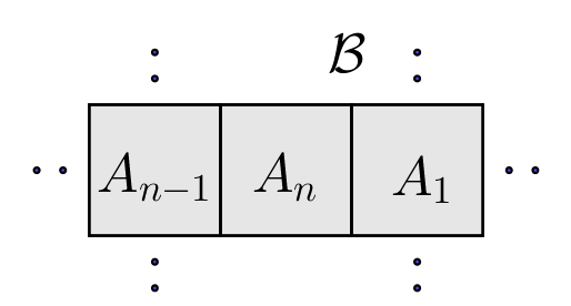
(a)

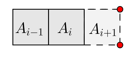
(b)

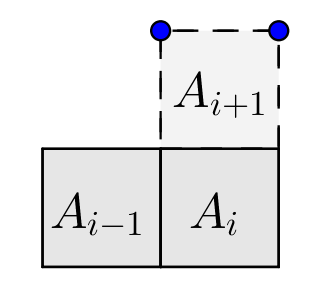
(c)

Figure 3.

∎

Let $\mathcal{P}$ be a polyomino. We set $S_{\mathcal{P}}=K[x_{v}\colon\;v\in V(\mathcal{P})]$, where $K$ is a field. If $[a,b]$ is an inner interval of $\mathcal{P}$, with $a$,$b$ and $c$,$d$ respectively diagonal and anti-diagonal corners, then the binomial $x_{a}x_{b}-x_{c}x_{d}$ is called an inner 2-minor of $\mathcal{P}$. We define $I_{\mathcal{P}}$ as the ideal in $S_{\mathcal{P}}$ generated by all the inner 2-minors of $\mathcal{P}$ and we call it the polyomino ideal of $\mathcal{P}$. We set also $K[\mathcal{P}]=S_{\mathcal{P}}/I_{\mathcal{P}}$, which is the coordinate ring of $\mathcal{P}$.

3. Krull dimension of closed path polyominoes

In this section we compute the Krull dimension of the coordinate ring attached to a closed path polyomino. We recall some basic facts on simplicial complexes. A finite simplicial complex $\Delta$ on the vertex set $[n]=\{1,\dots,n\}$ is a collection of subsets of $[n]$ satisfying the following two conditions:

1. if $F^{\prime}\in\Delta$ and $F\subseteq F^{\prime}$ then $F\in\Delta$;

2. $\{i\}\in\Delta$ for all $i=1,\dots,n$.

The elements of $\Delta$ are called faces, and the dimension of a face is one less than its cardinality. An edge of $\Delta$ is a face of dimension 1, while a vertex of $\Delta$ is a face of dimension 0. The maximal faces of $\Delta$ with respect to the set inclusion are called facets. The dimension of $\Delta$ is given by $\sup\{\dim(F):F\in\Delta\}$. We say that a simplicial complex $\Delta$ is pure if all facets have the same dimension. If $\Delta$ is pure, then the dimension of $\Delta$ is given trivially by the dimension of a facet of $\Delta$. Let $\Delta$ be a simplicial complex on $[n]$ and $R=K[x_{1},\dots,x_{n}]$ be the polynomial ring in $n$ variables over a field $K$. To every collection $F=\{i_{1},\dots,i_{r}\}$ of $r$ distinct vertices of $\Delta$, we associate a monomial $x^{F}$ in $R$ where $x^{F}=x_{i_{1}}\dots x_{i_{r}}.$ The monomial ideal generated by all monomials $x^{F}$ such that $F$ is not a face of $\Delta$ is called Stanley-Reisner ideal and it denoted by $I_{\Delta}$. The face ring of $\Delta$, denoted by $K[\Delta]$, is defined to be the quotient ring $R/I_{\Delta}$. It follows from [41, Corollary 6.3.5], if $\Delta$ is a simplicial complex on $[n]$ of dimension $d$, then $\dim K[\Delta]=d+1=\max\{s\colon\;x_{i_{1}}\dots x_{i_{s}}\notin I_{\Delta},i_{1}<\dots<i_{s}\}$.

Definition 3.1.

A polyomino $\mathcal{R}$ is called $\Gamma$-path with middle cell $D$ and hooking vertex $w$ if it consists of a maximal horizontal block $\mathcal{B}_{1}=[C_{1},B_{1}]$ of rank greater than three and a maximal vertical block $\mathcal{B}_{2}=[B_{2},C_{2}]$ of rank greater than three such that there is a cell $D$ not belonging to $\mathcal{B}_{1}\cup\mathcal{B}_{2}$ and $V(\mathcal{B}_{1})\cap V(\mathcal{B}_{2})=\{w\}$ where $w$ is the upper left corner of $D$. This is illustrated in Figure  4 (A). With reference to Figure 4, we define $\tau$-paths, $W$-paths and $\zeta$-paths in a similar way.

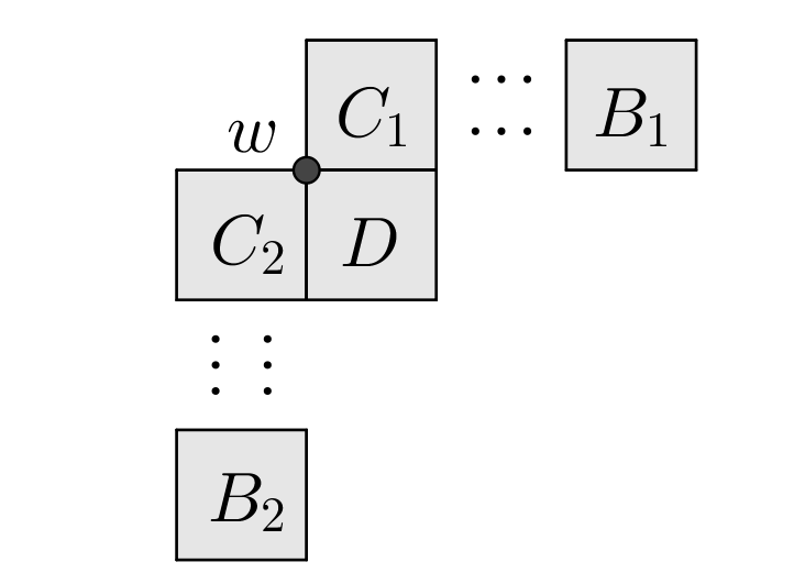
(a) $\Gamma$-path

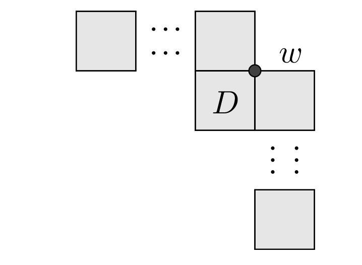
(b) $\tau$-path

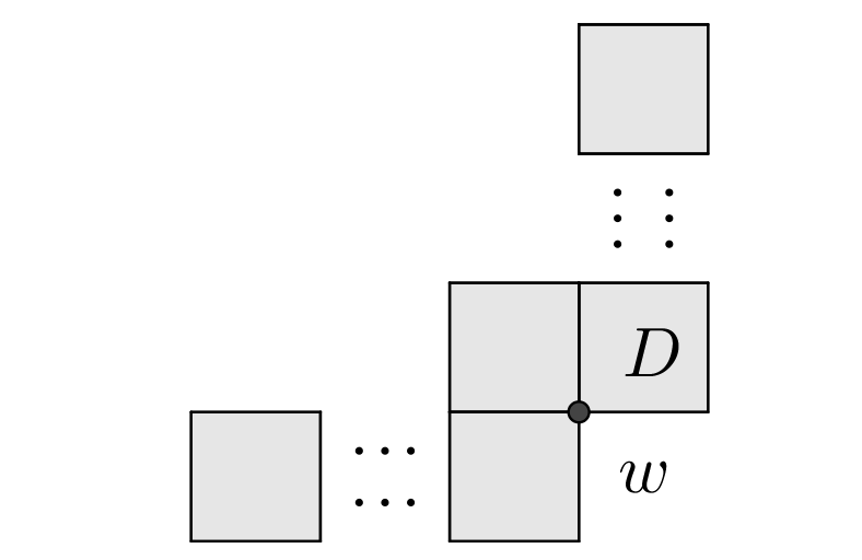
(c) $W$-path

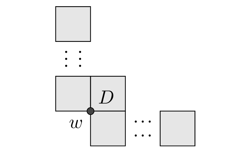
(d) $\zeta$-path

Figure 4.

Moreover, we say that a pair $(\mathcal{F},\mathcal{G})$ of the previous polyominoes is compatible if $\mathcal{F}$ is a $\Gamma$-path ($\tau$-path or $W$-path or $\zeta$-path) and $\mathcal{G}$ is one of the other paths.

Definition 3.2.

A polyomino $\mathcal{S}$ is called a LU-skew path with hooking vertices $a,b$ if it is made up of two maximal blocks $\mathcal{B}_{1}=[C_{1},D_{1}]$ and $\mathcal{B}_{2}=[C_{2},D_{2}]$, both of them having rank greater than three, with $V(\mathcal{B}_{1})\cap V(\mathcal{B}_{2})=\{a,b\}$ where $a,b$ are the left and right upper corners of $D_{1}$, respectively. For instance, see Figure LABEL:Figure:configurations_of_Skew (A). With reference to Figure LABEL:Figure:configurations_of_Skew, we can define $LD$-skew, $DU$-skew and $UD$-skew paths in a similar way.

Let $\mathcal{P}$ be a closed path and $(\mathcal{F},\mathcal{G})$ be a pair of two sub-polyominoes of $\mathcal{P}$ as in Definition 3.1. Without loss of generality, we may assume that the middle cell of $\mathcal{F}$ is $A_{1}$ and the middle cell of $\mathcal{G}$ is $A_{k}$ with $k\in[n-1]$. Then a sub-polyomino $\mathcal{Q}$ of $\mathcal{P}$ as in Definition 3.2 is said to be between $\mathcal{F}$ and $\mathcal{G}$ if $\mathcal{Q}$ is contained in $\{A_{i}:1<i<k\}$.
In the following remark we point out the structure of a closed path $\mathcal{P}$ having a zig-zag walk, showing that $\mathcal{P}$ consists of the configurations defined in Definitions 3.1 and 3.2, arranged in a suitable way. The latter is essentially a technical consequence of the characterization given in [3, Section 6] which states that a closed path has a zig-zag walk if and only if it has neither an $L$-configuration nor a ladder of at least three steps.

Remark 3.3.

Let $\mathcal{P}$ be a closed path with a zig-zag walk. We denote by $\mathcal{B}_{1}$ a maximal block of $\mathcal{P}$ having its length of at least three. It is not restrictive to assume that $\mathcal{B}_{1}=[A_{1},A_{k}]$, where $k\geq 3$, is in horizontal position and that $A_{n}$ is at North of $A_{1}$; otherwise we can rotate $\mathcal{P}$ suitably or relabel the cells of $\mathcal{P}$. Observe that $A_{n-1}$ is necessarily at West of $A_{n}$, otherwise if it is at North then $\mathcal{B}_{1}\cup\{A_{n-1},A_{n}\}$ contains an $L$-configuration. Consider now $A_{k+1}$ and note that it is at North of $A_{k}$ because it cannot be at East from the maximality of $\mathcal{B}_{1}$ and it cannot be at South otherwise either $\mathcal{B}_{1}\cup\{A_{k+1},A_{k+2}\}$ contains an $L$-configuration if $A_{k+2}$ is at South of $A_{k+1}$ or $\{A_{n-1},A_{n}\}\cup\mathcal{B}_{1}\cup\{A_{k+1},A_{k+2}\}$ is contained in a ladder of three steps if $A_{k+2}$ is at East of $A_{k+1}$. For similar arguments $A_{k+2}$ is necessarily at East of $A_{k+1}$. Now, we want to define inductively the configurations of cells that appear in $\mathcal{P}$, starting from $\mathcal{B}_{1}$. Set $h\geq 1$. Let $\mathcal{B}_{h}$ be a maximal block with at least three cells and we may assume that $\mathcal{B}_{h}=[A_{j_{h}},A_{j_{h+1}}]$, where $k<j_{h}<j_{h+1}<n$, is in horizontal position and that $A_{j_{h}-1}$ is at North of $A_{j_{h}}$, otherwise it is sufficient to reflect $\mathcal{P}$. For arguments similar to the ones done before, we can define the maximal block $\mathcal{B}_{h+1}=[A_{j_{h+2}},A_{j_{h+3}}]$ of $\mathcal{P}$ having at least three cells, arranged to $\mathcal{B}_{h}$ following Figure 6.

(a)

(b)

Figure 6. Arrangements of $\mathcal{B}_{h}$ and $\mathcal{B}_{h+1}$.

Since $\mathcal{P}$ is a closed path, this procedure is finite so there exists $t\in{\mathbb{N}}$ such that $\mathcal{B}_{t+1}=\mathcal{B}_{1}$ and $\mathcal{B}_{t}$ and $\mathcal{B}_{1}$ are arranged as in Figure 7.

(a)

(b)

Figure 7. Arrangements of $\mathcal{B}_{t}$ and $\mathcal{B}_{1}$.

Let $\mathcal{P}$ be a closed path polyomino. Let $<^{1}$ be the total order on $V(\mathcal{P})$ defined as $u<^{1}v$ if and only if, for $u=(i,j)$ and $v=(k,l)$, $i<k$, or $i=k$ and $j<l$. Let $Y\subset V(\mathcal{P})$ and consider $<^{Y}_{\mathrm{lex}}$ be the lexicographical order in $S_{\mathcal{P}}$ induced by the following order on the variables of $S_{\mathcal{P}}$:

$$\mbox{for}\ u,v\in V(\mathcal{P})\qquad x_{u}<^{Y}_{\mathrm{lex}}x_{v}\Leftrightarrow\left\{\begin{array}[]{l}u\notin Y\ \mbox{and}\ v\in Y\\ u,v\notin Y\ \mbox{and}\ u<^{1}v\\ u,v\in Y\ \mbox{and}\ u<^{1}v\end{array}\right.$$

From [7, Theorem 4.9], we know that there exists a suitable set $Y\subset V(\mathcal{P})$ such that the set of generators of $I_{\mathcal{P}}$ forms the reduced Gröbner basis of $I_{\mathcal{P}}$ with respect to $<^{Y}_{\mathrm{lex}}$, defined in [7, Algorithm 4.7, Definition 4.8]. The square-free monomial ideal $J_{\mathcal{P}}=\mathrm{in}_{<^{Y}_{\mathrm{lex}}}(I_{\mathcal{P}})$ can be viewed as the Stanley-Reisner ideal of a simplicial complex $\Delta(\mathcal{P})$ on the vertex set of $\mathcal{P}$.

Theorem 3.4.

Let $\mathcal{P}$ be a closed path and $\Delta(\mathcal{P})$ be the associated simplicial complex. Then $\Delta(\mathcal{P})$ is pure and the Krull dimension of $K[\mathcal{P}]$ is $|V(\mathcal{P})|-\mathrm{rank}(\mathcal{P})$.

Proof.

Firstly, we assume that $\mathcal{P}$ does not contain any zig-zag walk. We know that $I_{\mathcal{P}}$ is a toric ideal from [3, Theorem 6.2], so $\Delta_{\mathcal{P}}$ is pure from [41, Theorem 9.6.1]. Moreover, from [8, Theorem 5.5], the Krull dimension is given by $|V(\mathcal{P})|-\mathrm{rank}(\mathcal{P})$.
We need to examine only the case when $\mathcal{P}$ contains a zig-zag walk. Suppose that we are in this case. Hence, in what follows, our aim is to define a suitable facet of $\Delta(\mathcal{P})$. We have that $\mathcal{P}$ contains just the configurations defined in Definitions 3.1 and 3.2, arranged as described in Remark 3.3. Let $\mathcal{S}_{1}$ be a $\Gamma$-path. Referring to Figure 4 (A), we label the cells of $\mathcal{P}$ setting $D=A_{1}$, $C_{1}=A_{2}$ and so on. Let $k>1$ be the minimum integer such that $\mathcal{S}_{2}$ is either a $W$-path or a $\tau$-path with middle cell $A_{k}$. The hooking vertices of $\mathcal{S}_{1}$ and $\mathcal{S}_{2}$ are on the same maximal horizontal edge interval $V$ of $\mathcal{P}$ and, if there exist, the hooking vertices of the $LU$-skew or $LD$-skew paths between $\mathcal{S}_{1}$ and $\mathcal{S}_{2}$ belong to $V$. Moreover, by the minimality of $k$, there does not exist any $DU$-skew and $UD$-skew path between $\mathcal{S}_{1}$ and $\mathcal{S}_{2}$ belonging to $V$. We want to define a suitable set of vertices of $\mathcal{P}$ in order to find a facet of $\Delta(\mathcal{P})$. We distinguish two cases, depending if $\mathcal{S}_{2}$ is a $W$-path or a $\tau$-path. We may consider $z_{T},x_{T}\in Y$ and $y_{T}\notin Y$, with reference to Figure 8.
Case I: Assume that $\mathcal{S}_{2}$ is a $W$-path.

1. Suppose that there does not exist any $LU$-skew or $LD$-skew paths between $\mathcal{S}_{1}$ and $\mathcal{S}_{2}$. Let $\mathcal{B}_{1}$ be the maximal horizontal block $[A_{2},A_{k-1}]$. Denote the upper right corner of $A_{i}$ by $a_{i}^{1}$ for all $i=2,\dots,k-1$ and the upper left corner of $A_{2}$ by $a_{1}^{1}$. We set

   $$V(\mathcal{S}_{1},\mathcal{S}_{2})=\{a_{i}^{1}:i\in[\mathrm{rank}(\mathcal{B}_{1})]\},$$

   as in Figure 8.

   

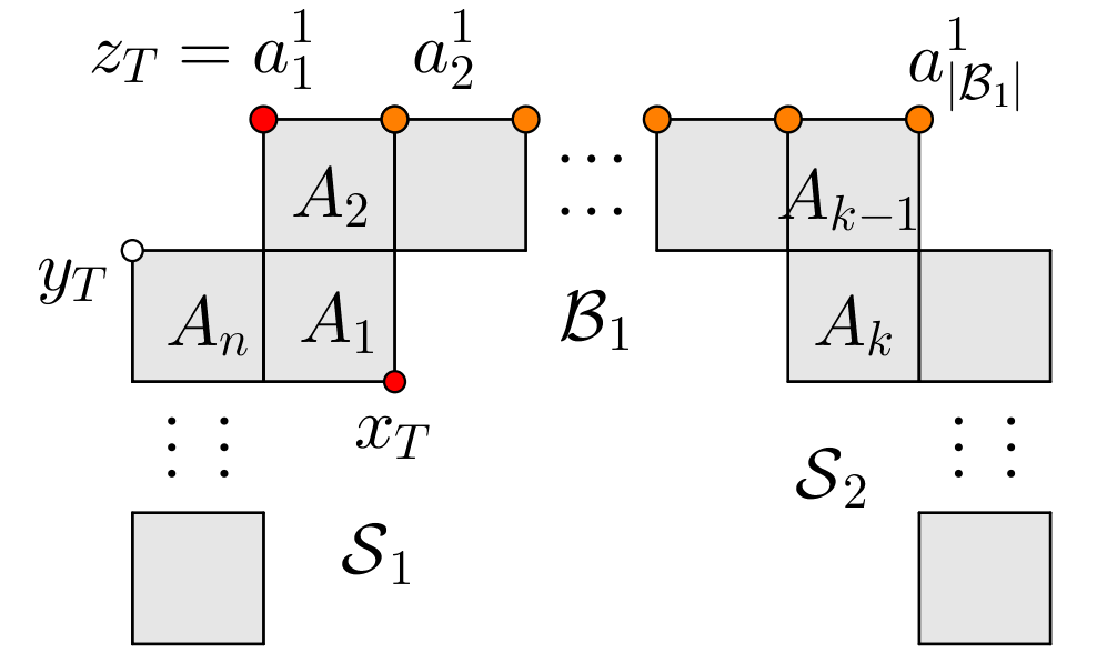
   Figure 8.

2. Suppose that there exist $LD$-skew or $LU$-skew paths between $\mathcal{S}_{1}$ and $\mathcal{S}_{2}$ and, in particular, that there are $m$ maximal horizontal blocks $\mathcal{B}_{i}$ between $\mathcal{S}_{1}$ and $\mathcal{S}_{2}$. Set $\mathcal{B}_{j}=[A_{k_{j}},A_{k_{j+1}}]$, where $k_{1}=2$ and $k_{j}<k_{j+1}$ for all $j\in[m]$. For all $j\in[m]$ odd and for all $i=1,\dots,\mathrm{rank}(\mathcal{B}_{j})$, we denote by $a_{1}^{j}$ the upper left corner of $A_{k_{j}}$ and by $a_{i}^{j}$ the right upper corner of $A_{k_{j}+i}$ in $\mathcal{B}_{j}$. For all $j\in[m]$ even and for all $i=1,\dots,\mathrm{rank}(\mathcal{B}_{j})$, we denote by $a_{i}^{j}$ the lower right corner of $A_{k_{j}+i}$ in $\mathcal{B}_{j}$. See Figure 9.

   

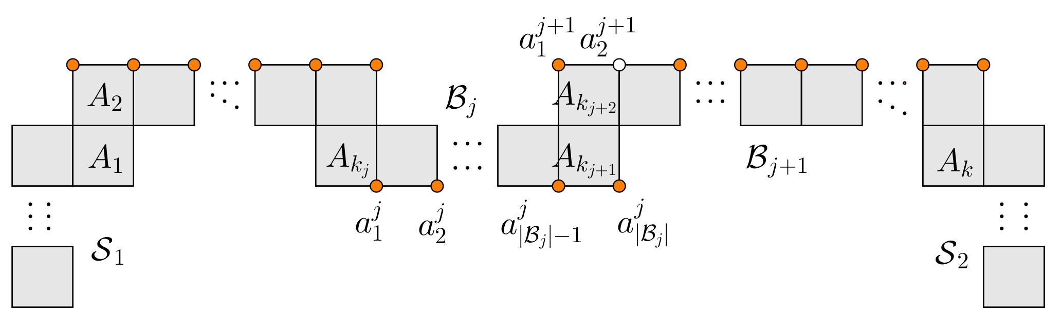
   Figure 9.

   Recall that for all $j\in[m]$, $a^{j}_{|\mathcal{B}_{j}|-2},a^{j}_{|\mathcal{B}_{j}|-1}\notin Y$ and $a^{j+1}_{1},a^{j+1}_{2}\in Y$ with $a^{j+1}_{2}>a^{j+1}_{1}$. Then we set

   $$V(\mathcal{S}_{1},\mathcal{S}_{2})=\bigcup_{j\in[m]\atop even}\{a_{i}^{j}:i\in[\mathrm{rank}(\mathcal{B}_{j})]\}\cup\biggl{(}\bigcup_{j\in[m]\atop odd}\{a_{i}^{j}:i\in[\mathrm{rank}(\mathcal{B}_{j})+1]\}\biggr{)}\backslash\bigcup_{j\in[m]\atop odd}\{a_{2}^{j}\}.$$

Case II: Assume that $\mathcal{S}_{2}$ is a $\tau$-path.

1. Suppose that there exists just an $LD$-skew path between $\mathcal{S}_{1}$ and $\mathcal{S}_{2}$. For all $i=0,\dots,\mathrm{rank}(\mathcal{B}_{1})-1$, we denote by $a_{1}^{1}$ the upper left corner of $A_{2}$ and by $a_{i}^{1}$ the right upper corner of $A_{k_{j}+i}$ in $\mathcal{B}_{j}$. For all $i=1,\dots,\mathrm{rank}(\mathcal{B}_{2})-1$, we denote by $a_{i}^{2}$ the lower right corner of $A_{t+i}$ in $\mathcal{B}_{2}$. See Figure 10. In this case, we set

   $$V(\mathcal{S}_{1},\mathcal{S}_{2})=\{a_{i}^{1}:i\in[\mathrm{rank}(\mathcal{B}_{1})]\}\cup\{a_{i}^{2}:i\in[\mathrm{rank}(\mathcal{B}_{2})]\}.$$

   

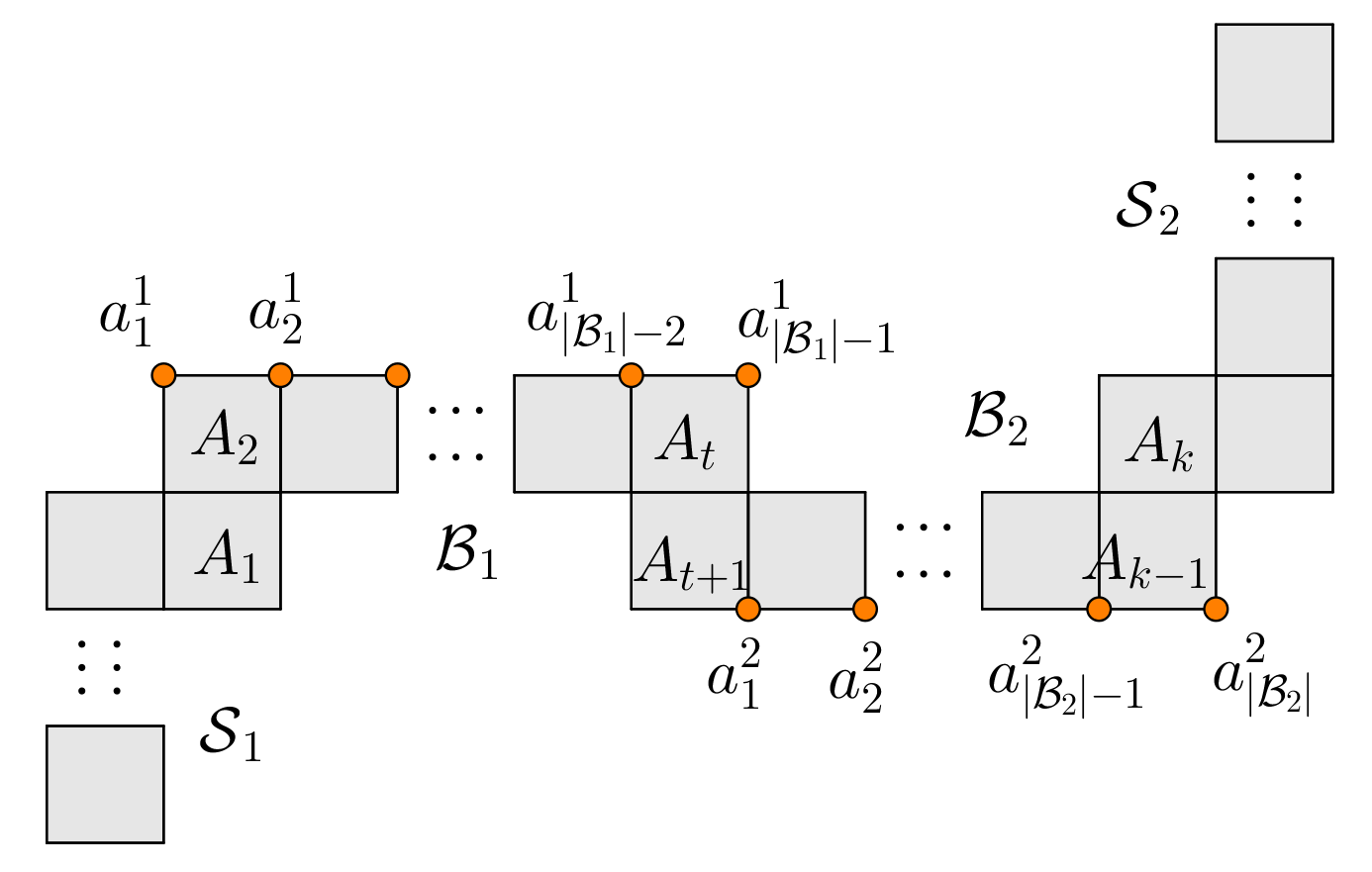
   Figure 10.

2. Suppose that there exist $LD$-skew or $LU$-skew paths between $\mathcal{S}_{1}$ and $\mathcal{S}_{2}$. With the same notations as in (2) of Case I (see Figure 11), we set

   $$V(\mathcal{S}_{1},\mathcal{S}_{2})=\bigcup_{j\in[m]\atop even}\{a_{i}^{j}:i\in[\mathrm{rank}(\mathcal{B}_{j})]\}\cup\biggl{(}\bigcup_{j\in[m]\atop odd}\{a_{i}^{j}:i\in[\mathrm{rank}(\mathcal{B}_{j})]\}\biggr{)}\backslash\bigcup_{j\in[m]\atop odd}\{a_{2}^{j}\}.$$

   

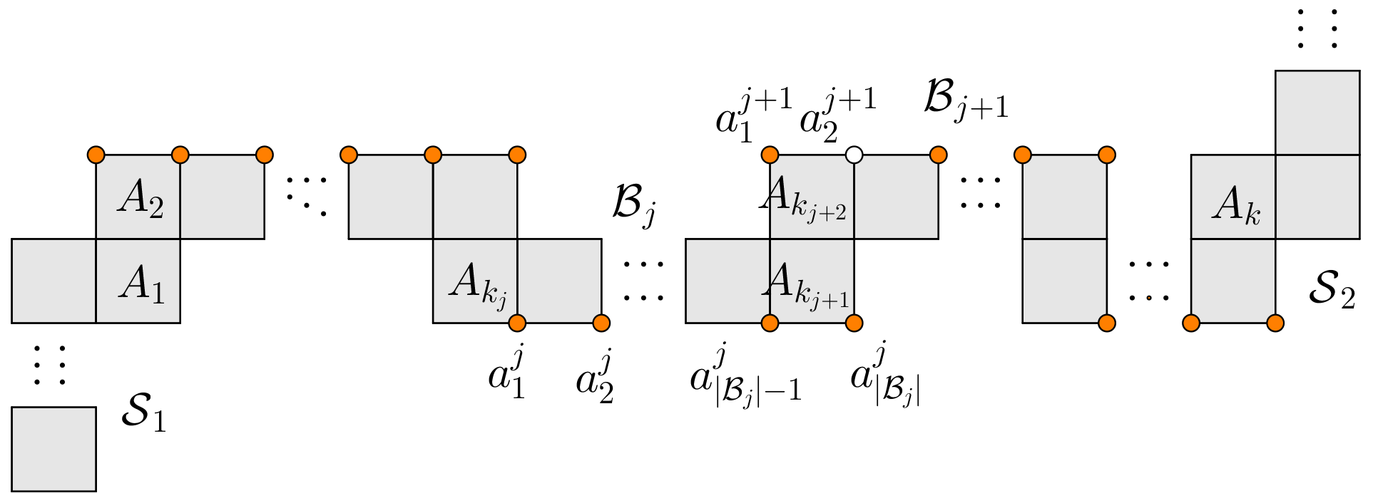
   Figure 11.

In each case, we can define the following bijective correspondence $\phi_{1,2}:V(\mathcal{S}_{1},\mathcal{S}_{2})\rightarrow\{A_{1}\}\cup\bigcup_{i=1}^{m}\mathcal{B}_{i}$ with $\phi_{1,2}(a_{1}^{1})=A_{1}$ and $\phi_{1,2}(a_{i}^{j})=A_{k_{j}+i}$ all $j\in[m]$ and for all $i\in[\mathrm{rank}(\mathcal{B}_{j})]$; in particular, $|V(\mathcal{S}_{1},\mathcal{S}_{2})|=\sum_{i=1}^{m}\mathrm{rank}(\mathcal{B}_{i})+1$. Once we have defined the set $V(\mathcal{S}_{1},\mathcal{S}_{2})$, we can use the same arguments for all pairs $(\mathcal{S}_{i},\mathcal{S}_{i+1})$ of compatible paths, where $\mathcal{S}_{i+1}$ is taken by minimality with respect $\mathcal{S}_{i}$, as done for $(\mathcal{S}_{1},\mathcal{S}_{2})$. Assume that there exist $t$ such pairs, where $\mathcal{S}_{t+1}=\mathcal{S}_{1}$. So as done before, for all $i\in[t]$, we can define $V(\mathcal{S}_{i},\mathcal{S}_{i+1})$ by similar arguments as for $V(\mathcal{S}_{1},\mathcal{S}_{2})$. Hence, $V=\cup_{i=1}^{t}V(\mathcal{S}_{i},\mathcal{S}_{i+1})$. Observe that $|V|=\mathrm{rank}(\mathcal{P})$. We want to prove that $F=\{x_{v}:v\in V\}$ is a facet of $\Delta(\mathcal{P})$. Obviously, $F$ is a face of $\Delta(\mathcal{P})$, so we need to prove the maximality with respect to the set inclusion. Suppose, by contradiction, that $F$ is not maximal. Then there exists a $p\in V(\mathcal{P})\backslash V$ such that $F\subset F\cup\{x_{p}\}$. Without loss of generality, we may assume that $p$ is a vertex of the sub-polyomino $\{A_{1}\}\cup\bigcup_{i=1}^{m}\mathcal{B}_{i}$ between $\mathcal{S}_{1}$ and $\mathcal{S}_{2}$.

1. Assume that we are in $(1)$ of Case I. Suppose $p\in V(\mathcal{B}_{1})$. If $p$ is the lower left corner of $A_{2}$, then since $y_{T}\notin Y$, we get the contradiction that $x_{p}x_{q}\in J_{\mathcal{P}}$, where $q$ is the lower left corner of $A_{n}$. In the other cases, we obtain similarly a contradiction considering $\{x_{a_{1}^{1}},x_{p}\}$, as well as when $p$ is the lower left or right corner of $A_{1}$.

2. Assume that we are in $(2)$ of Case I. The only case which we discuss is when $p=a_{2}^{j+1}$ for some $j\in[m]$. In this case, since $a_{2}^{j+1}>a_{1}^{j+1}$ we have $x_{a^{j}_{|\mathcal{B}_{j}|-1}}x_{a_{2}^{j+1}}\in J_{\mathcal{P}}$. But $\{x_{a^{j}_{|\mathcal{B}_{j}|-1}},x_{a_{2}^{j+1}}\}\in\Delta(\mathcal{P})$ since $p=a_{2}^{j+1}$, so we get a contradiction.

3. In the subcases $(1)$ and $(2)$ of Case II, we can argue in a similar way, and we obtain a contradiction.

Therefore, $F$ is a facet of $\Delta(\mathcal{P})$. Now, we prove that all other facets of $\Delta(\mathcal{P})$ can be obtained from $F$ replacing some vertices of $F$ with other ones in the same number. Let $G$ be a facet of $\Delta(\mathcal{P})$. Since $\mathcal{P}$ is union of the configurations defined in Definitions 3.1 and 3.2, arranged suitably as explained in Remark 3.3, it is sufficient to study the behavior of $G$ in the cases described in Figures 8, 9, 10, 11. Without losing of generality, we may examine the case in Figure 8 and, with reference to Figure 12, it is sufficient to focus on the vertices $\mathcal{L}=\{a_{i},b_{i}\}_{i\in[n]}\cup\{c_{1},c_{2},e,w,f,g,d_{1},d_{2}\}$ (where $[n]=\{1,\dots,n\}$). Note that the orange vertices are the points of $F$ belonging to the vertical cell intervals $\mathcal{B}_{2}$ and $\mathcal{B}_{3}$. Moreover, we remember that $c_{1}$, $d_{m-1}$ and $d_{m}$ cannot belong to $Y$, because $a_{1}=z_{T}$ and $w=x_{T}$ are in $Y$.

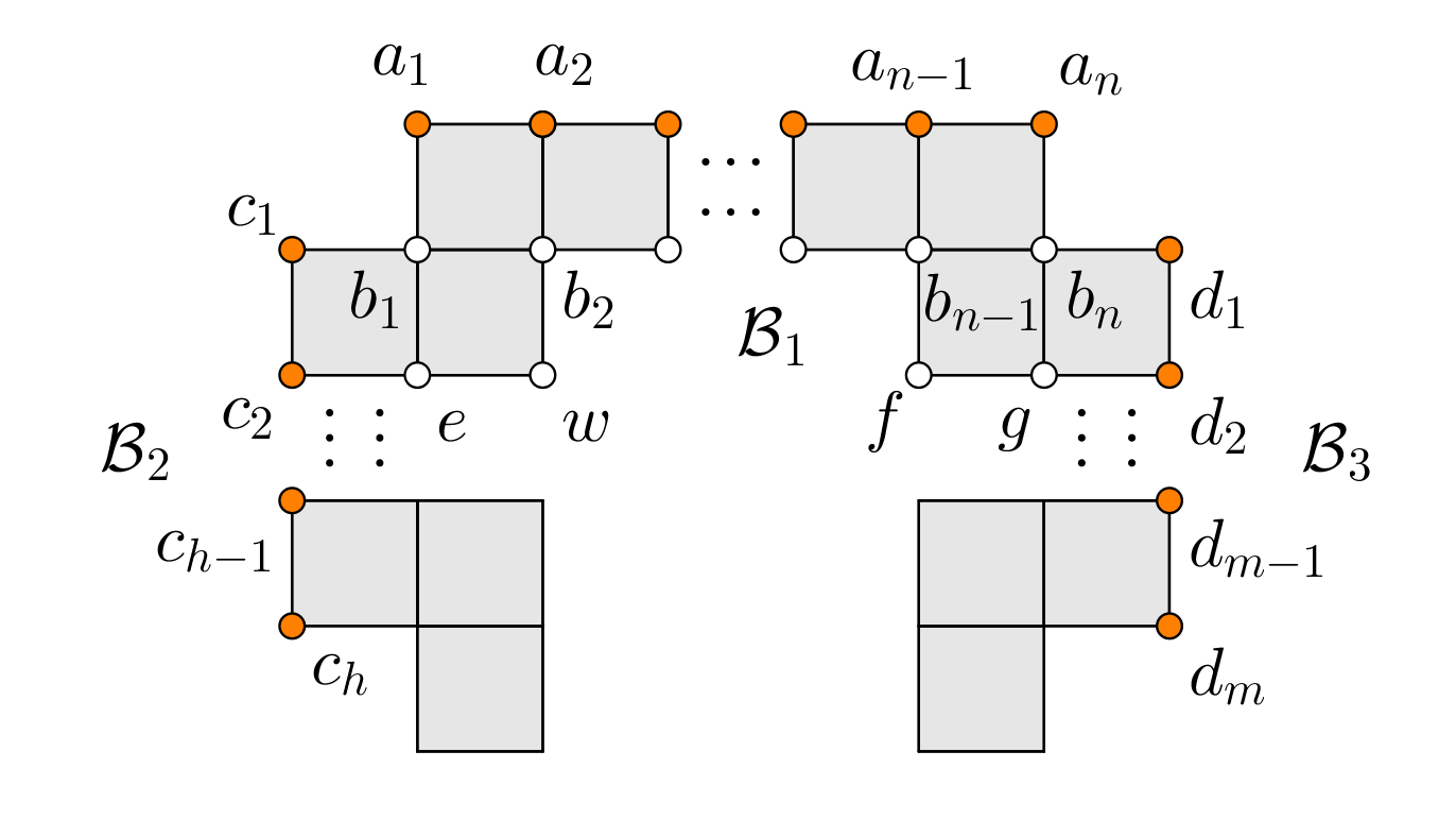
Figure 12.

Observe that we cannot replace $a_{1}$ in $F$ with a $b_{i}$ for $i\in\{2,\dots,n-1\}$, otherwise $\{b_{i},a_{i+1}\}\in\Delta(\mathcal{P})$, a contradiction. A similar conclusion, that is $\{c_{2},b_{1}\}\in\Delta(\mathcal{P})$, arises if we replace $a_{1}$ with $b_{1}$ in $F$. Moreover, note that if $a_{1}\in G$, then we cannot replace any point in $\mathcal{L}\setminus\{a_{1}\}$ with another one, otherwise we get a contradiction similar to the previous one. The only possibilities for $G$ are described in the following:

1. $G=F\setminus\{a_{1}\}\cup\{b_{n}\}$;

2. $G\in\{H_{i}:i\in\{2,\dots,n\}\}$, where

   $$H_{i}=F\setminus\big{(}\{a_{1}\}\cup\{a_{k}:k\in\{i+1,\dots,n\}\}\big{)}\cup\big{(}\{b_{n}\}\cup\{b_{k}:k\in\{i,\dots,n-1\}\}\big{)};$$

3. $G\in\{K_{i}:i\in\{2,\dots,n\}\}$, where $K_{i}=H_{i}\setminus\{b_{n},d_{1}\}\cup\{f,g\};$

4. $G=F\setminus\{a_{1},c_{1}\}\cup\{b_{n},w\}$;

5. $G\in\{P_{i}:i\in\{2,\dots,n\}\}$, where

   $$P_{i}=F\setminus\big{(}\{a_{1},c_{1}\}\cup\{a_{k}:k\in\{i+1,\dots,n\}\}\big{)}\cup\big{(}\{w,b_{n}\}\cup\{b_{k}:k\in\{i,\dots,n-1\}\}\big{)};$$

6. $G\in\{Q_{i}:i\in\{2,\dots,n\}\}$, where $Q_{i}=P_{i}\setminus\{b_{n},d_{1}\}\cup\{f,g\}.$

In each of the presented cases, we have $|G|=|F|$. In general, we can extend the previous arguments to each part of $\mathcal{P}$, and we always obtain that $|G|=|F|$. Therefore, there does not exist any facet $G$ in $\Delta(\mathcal{P})$ such that $|G|>\mathrm{rank}(\mathcal{P})$ or $|G|<\mathrm{rank}(\mathcal{P})$. Hence, all facets in $\Delta(\mathcal{P})$ have the same dimension, so $\Delta(\mathcal{P})$ is pure. Moreover, $\dim\Delta(\mathcal{P})=\mathrm{rank}(\mathcal{P})-1$, so $\dim K[\mathcal{P}]=\mathrm{rank}(\mathcal{P})$. From Lemma 2.1, we obtain that $\dim K[\mathcal{P}]~{}=|V(\mathcal{P})|-\mathrm{rank}(\mathcal{P})$. ∎

Corollary 3.5.

Let $\mathcal{P}$ be a closed path polyomino. Then $\mathrm{ht}(I_{\mathcal{P}})=\mathop{\rm rank}\nolimits(\mathcal{P})$.

Proof.

It follows from Theorem 3.4 and [41, Corollary 3.1.7]. ∎

It is known that if $\mathcal{P}$ is a simple polyomino, then $\dim(K[\mathcal{P}])=|V(\mathcal{P})|-\mathop{\rm rank}\nolimits(\mathcal{P})$, so $\mathrm{ht}(I_{\mathcal{P}})=\mathop{\rm rank}\nolimits(\mathcal{P})$. Arises naturally the following conjecture.

Conjecture 3.6.

Let $\mathcal{P}$ be a non-simple polyomino. Then $\mathrm{ht}(I_{\mathcal{P}})=\mathop{\rm rank}\nolimits(\mathcal{P})$.

4. Closed paths and Kőnig type property

Let $R=K[x_{1},\dots,x_{n}]$ and $I$ be a graded ideal in $R$ of height $h$. In according to [22], we say that $I$ is of Kőnig type if the following two conditions hold:

1. there exists a sequence $f_{1},\dots,f_{h}$ of homogeneous polynomials forming part of a minimal system of homogeneous generators of $I$;

2. there exists a monomial order $<$ on $R$ such that $\mathop{\rm in}\nolimits_{<}(f_{1}),\dots,\mathop{\rm in}\nolimits_{<}(f_{h})$ is a regular sequence.

If $\mathcal{P}$ is a polyomino and $I_{\mathcal{P}}$ is its polyomino ideal, then we say that $\mathcal{P}$ is of Kőnig type if $I_{\mathcal{P}}$ is an ideal of Kőnig type. In [21] it is proved that all simple thin polyominoes are of Kőnig type. Obviously, a closed path is a thin and non-simple polyomino. The aim of this section is to show that also this class of polyominoes satisfies this property.

Remark 4.1.

We point out that the polyomino ideal of a thin polyomino is not always of Kőnig type. To illustrate this, we consider the polyomino $\mathcal{P}$ from Figure  13. Using the Algebra software Macaulay2 ([4, 14]) we compute the height of $I_{\mathcal{P}}$, and we obtain that $\mathrm{ht}(I_{\mathcal{P}})=13=\mathop{\rm rank}\nolimits(\mathcal{P})$, as expected. Note that $|V(\mathcal{P})|=24$, so $|V(\mathcal{P})|<2\mathop{\rm rank}\nolimits(\mathcal{P})$. Hence $I_{\mathcal{P}}$ cannot be of Kőnig type.

Figure 13.

Remark 4.2.

Let $\mathcal{P}$ be a closed path polyomino having $n$ distinct cells. Let $<_{\mathrm{lex}}$ be the lexicographic order induced by a total order on $\{x_{v}:v\in V(\mathcal{P})\}$. Suppose that there exist $n$ generators $f_{1},\dots,f_{n}$ of $I_{\mathcal{P}}$ whose initial terms do not have any variable in common. Then, from Corollary 3.5, we know that $\mathrm{ht}(I_{\mathcal{P}})=n$. Moreover, $\gcd(\mathop{\rm in}\nolimits_{<_{\mathrm{lex}}}(f_{i}),\mathop{\rm in}\nolimits_{<_{\mathrm{lex}}}(f_{j}))=1$ for all $i\neq j$, so $\mathop{\rm in}\nolimits_{<_{\mathrm{lex}}}(f_{1}),\dots,\mathop{\rm in}\nolimits_{<_{\mathrm{lex}}}(f_{n})$ forms a regular sequence. Hence, $I_{\mathcal{P}}$ is of Kőnig type.

Definition 4.3.

Let $\mathcal{P}:A_{1},\dots,A_{n}$ be a closed path polyomino. In order to define a suitable total order on $\{x_{v}:v\in V(\mathcal{P})\}$, Table 1 will be very useful. Let $Y^{(1)}\subset V(\mathcal{P})$. Let $j\geq 2$ and assume that $Y^{(j-1)}$ is known. We want to define $Y^{(j)}$. We refer to Table 1 up to suitable rotations and reflections of $\mathcal{P}$. If one of the configurations in the left column of Table 1 occurs, where the blue vertices are in $Y^{(j-1)}$, then we denote by $k$ the maximum integer such that $m+k$ is an orange vertex in the picture displayed in the corresponding right column. Hence, we set $Z^{(j)}_{1}=\{x_{m},\dots,x_{m+k}\}$ and $Z^{(j)}_{2}=\{x_{m^{\prime}},\dots,x_{(m+k)^{\prime}}\}$, where for all $a\in Y^{(j-1)}_{1}$ we put $x_{a}>x_{h_{1}}>x_{h_{2}}>x_{1^{\prime}}$ with $m<h_{1}<h_{2}\leq m+k$ and for all $b\in Y^{(j-1)}_{2}$ we put $x_{b}>x_{t_{1}}>x_{t_{2}}$ with $m^{\prime}<t_{1}<t_{2}\leq(m+k)^{\prime}$. Therefore, we define $Y^{(j)}=Y^{(j)}_{1}\sqcup Y^{(j)}_{2}$ where $Y^{(j)}_{1}=Y^{(j-1)}_{1}\sqcup Z^{(j)}_{1}$ and $Y^{(j)}_{2}=Y^{(j-1)}_{2}\sqcup Z^{(j)}_{2}$.

	IF it occurs …	THEN we refer to …
I
II
III
IV
V
VI
VII
VIII
IX
X

Table 1.

We need to distinguish just two cases depending on the changes of direction in $\mathcal{P}$, so we have the following two results.

Proposition 4.4.

Let $\mathcal{P}:A_{1},\dots,A_{n}$ be a closed path polyomino. Suppose that $\mathcal{P}$ contains a configuration of four cells as in Figure 14 (A), up to reflections or rotations of $\mathcal{P}$ or up to relabelling of the cells of $\mathcal{P}$. Then $I_{\mathcal{P}}$ is of Kőnig type.

Proof.

We distinguish two cases depending on the position of $A_{3}$ with respect to $A_{2}$.
Case I: We assume that $A_{3}$ is at North of $A_{2}$.

(a)

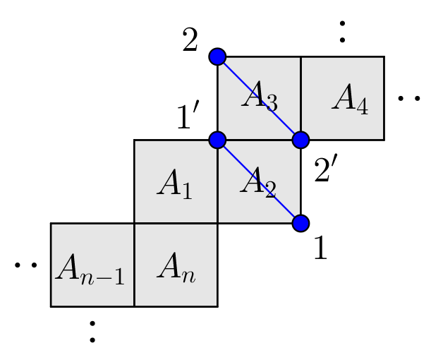
(b)

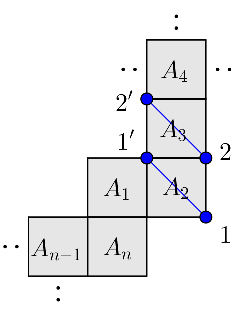
(c)

Figure 14.

We set $Y^{(1)}=Y^{(1)}_{1}\sqcup Y^{(1)}_{2}$ where $Y^{(1)}_{1}=\{x_{1},x_{2}\}$ and $Y^{(1)}_{2}=\{x_{1^{\prime}},x_{2^{\prime}}\}$ with $x_{1}>x_{2}>x_{1^{\prime}}>x_{2^{\prime}}$, with reference to Figure 14 (B) if $A_{4}$ is at East of $A_{3}$ or to Figure  14 (C) if $A_{4}$ is at North of $A_{3}$. Starting with this position for $Y^{(1)}$, we apply the procedure described in Definition 4.3.

Since $\mathcal{P}$ has a finite number of cells and stopping it in the configuration $\{A_{n-1},A_{n},A_{1},A_{2}\}$, the previous procedure consists of a finite number of steps, let us say $p$ steps. In particular, in Figure 15, we summarize all cases which may appear in the last step, where the blue vertices represent the points which are in $Y^{(p-1)}$ in the penultimate step. Let $Y=Y^{(p)}$ be the order set of variables obtained by using the previous arguments and let $|Y|=2r$ with $r\in{\mathbb{N}}$. We have $x_{1}>x_{2}>\dots>x_{r}>x_{1^{\prime}}>x_{2^{\prime}}>\dots>x_{r^{\prime}}$ and we set $Y_{1}=\{x_{1},x_{2},\dots,x_{r}\}$ and $Y_{2}=\{x_{1^{\prime}},x_{2^{\prime}},\dots,x_{r^{\prime}}\}$. Moreover, observe that all vertices of $\mathcal{P}$ are covered two by two, so $r=n$ by Lemma 2.1. Hence, we obtain $n$ generators of $I_{\mathcal{P}}$ whose initial terms do not have any variables in common, hence, by Remark 4.2, it follows that $I_{\mathcal{P}}$ is of Kőnig type.

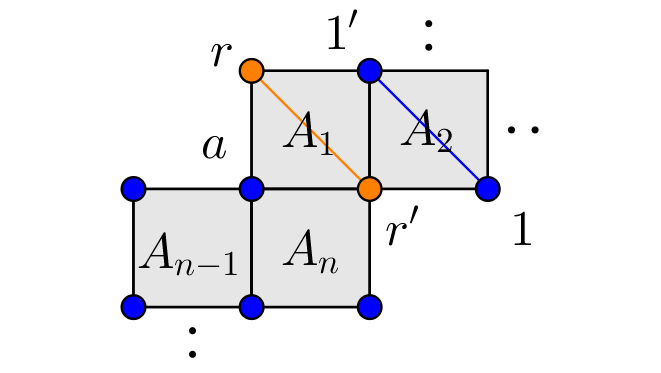
(a) Note $a\in Y_{2}$

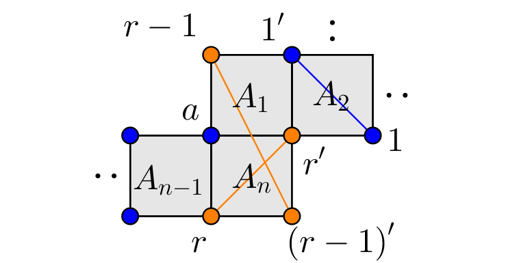
(b) Note $a\in Y_{2}$

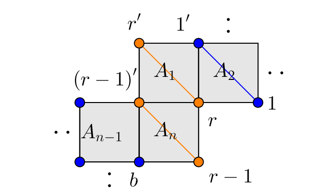
(c) Note $b\in Y_{2}$

Figure 15. The cases in the last step.

Case II: We assume that $A_{3}$ is at East of $A_{2}$. We set $Y^{(1)}=Y^{(1)}_{1}\sqcup Y^{(1)}_{2}$ where $Y^{(1)}_{1}=\{x_{1}\}$ and $Y^{(1)}_{2}=\{x_{1^{\prime}}\}$ with $x_{1}>x_{1^{\prime}}$, with reference to Figure  16 (A). As done before, we start with this position for $Y^{(1)}$ and we apply the procedure described in Definition 4.3. Let $q$ be the number of the steps until $\{A_{n-1},A_{n},A_{1},A_{2}\}$. In Figure 15 (A), (B) and (C) we show all cases in the last step and we point out that we set $x_{0}>x_{1}$. Hence, with the same arguments as before we get the desired conclusion.

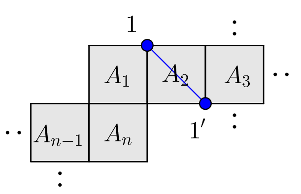
(a)

(b)

(c) Note $a\in Y_{2}$

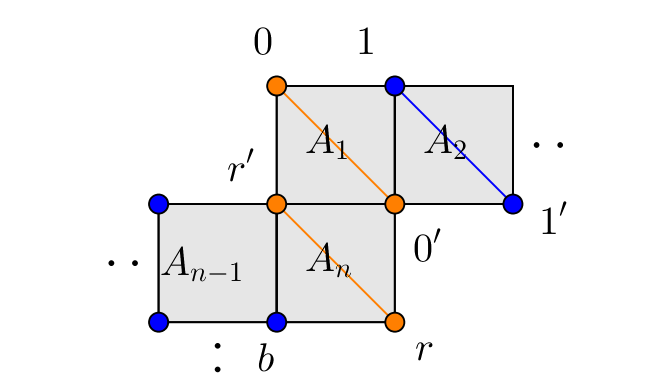
(d) Note $b\in Y_{2}$

Figure 16.

∎

Example 4.5.

An example of the procedure described in Lemma 4.4 can be seen in Figure 17. In particular, $\mathcal{P}$ is of Kőnig type with respect to the lexicographic order induced by

$$x_{1}>x_{2}>\dots>x_{30}>x_{1^{\prime}}>x_{2^{\prime}}>\dots>x_{30^{\prime}}$$

and to the thirty generators of $I_{\mathcal{P}}$ corresponding to the inner intervals having $i$ and $i^{\prime}$ as diagonal or anti-diagonal corners, for all $i\in[30]$.

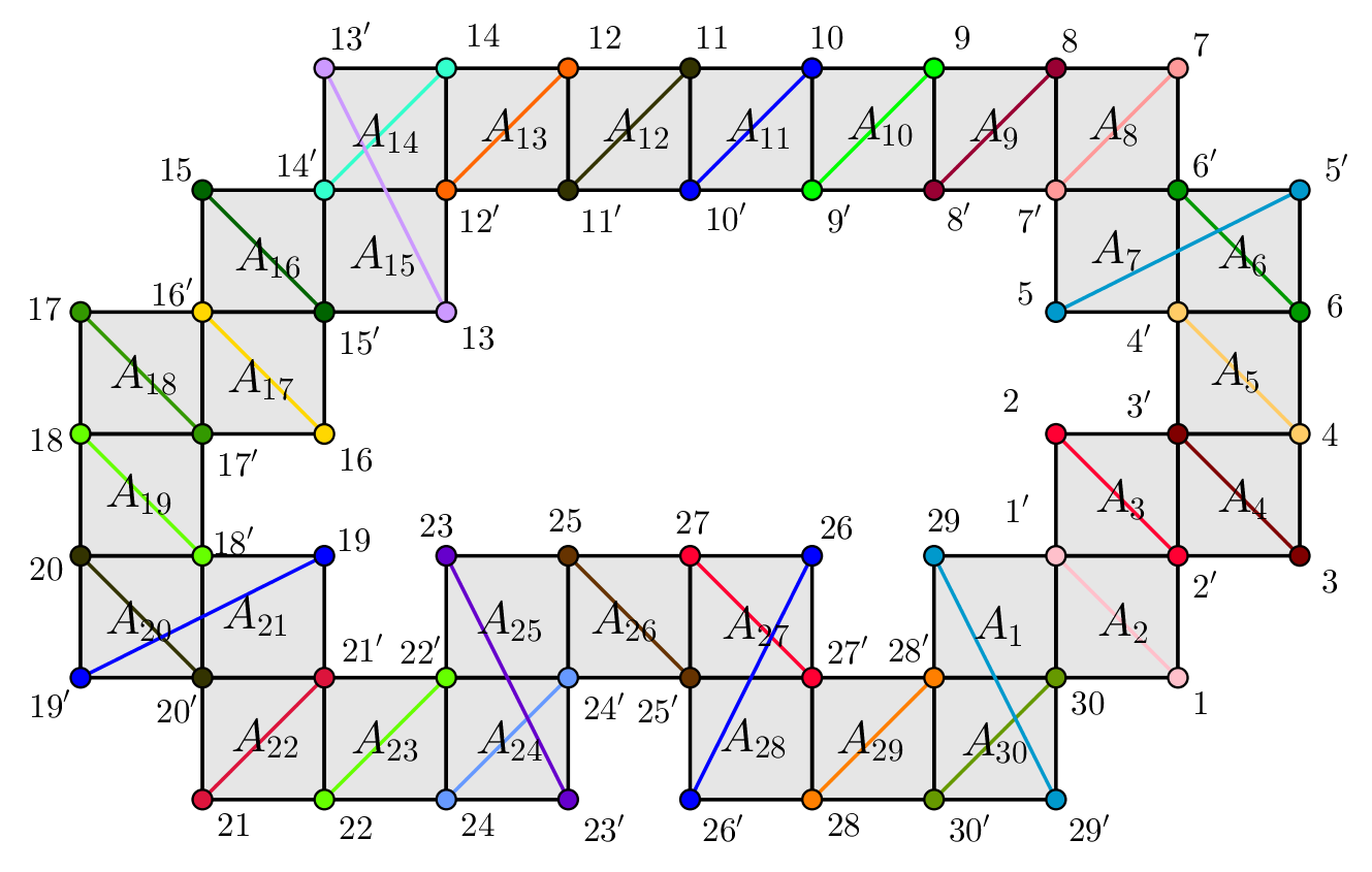
Figure 17.

We describe the algorithm given in Proposition 4.4 and we show how it works step by step, with reference to Figure 17.
Step 1. Starting from the tetromino $\{A_{1},A_{2},A_{3},A_{4}\}$, observe that $A_{4}$ is at East of $A_{3}$ so we are in the case of Figure 14 (B). Hence we set $Y^{(1)}=Y^{(1)}_{1}\sqcup Y^{(1)}_{2}$ with $Y^{(1)}_{1}=\{x_{1},x_{2}\}$ and $Y^{(1)}_{2}=\{x_{1^{\prime}},x_{2^{\prime}}\}$, where $x_{1}>x_{2}>x_{1^{\prime}}>x_{2^{\prime}}$.
Step 2. Consider now the tetromino $\{A_{3},A_{4},A_{5},A_{6}\}$, so it occurs the case (V) of Table 1. Hence we set $Y^{(2)}=Y^{(2)}_{1}\sqcup Y^{(2)}_{2}$ with $Y^{(2)}_{1}=Y^{(1)}_{1}\sqcup Z^{(2)}_{1}$ where $Z^{(2)}_{1}=\{x_{3},x_{4}\}$ and $Y^{(2)}_{2}=Y^{(1)}_{2}\sqcup Z^{(2)}_{2}$ where $Z^{(2)}_{2}=\{x_{3^{\prime}},x_{4^{\prime}}\}$, where $x_{1}>x_{2}>x_{3}>x_{4}>x_{1^{\prime}}>x_{2^{\prime}}>x_{3^{\prime}}>x_{4^{\prime}}$.
Step 3. Focusing on $\{A_{5},A_{6},A_{7},A_{8}\}$, we are in the case (III) of Table 1 after suitable rotations of $\mathcal{P}$. Hence $Z^{(3)}_{1}=\{x_{5},x_{6}\}$ and $Z^{(2)}_{2}=\{x_{5^{\prime}},x_{6^{\prime}}\}$, where $x_{1}>\dots>x_{4}>x_{5}>x_{6}>x_{1^{\prime}}>\dots>x_{4^{\prime}}>x_{5^{\prime}}>x_{6^{\prime}}$.
Step 4. Take the trimino $\{A_{8},A_{9},A_{10}\}$, so we have the case (I) of Table 1 after a reflection of $\mathcal{P}$ with respect to $y$-axis. Hence $Z^{(5)}_{1}=\{x_{8}\}$ and $Z^{(2)}_{2}=\{x_{8^{\prime}}\}$, with $x_{1}>\dots>x_{7}>x_{8}>x_{1^{\prime}}>\dots>x_{7^{\prime}}>x_{8^{\prime}}$.
Steps 5-9. We can argue as done in the previous step so we obtain $x_{1}>\dots>x_{11}>x_{12}>x_{1^{\prime}}>\dots>x_{11^{\prime}}>x_{12^{\prime}}$. From this point, it should be clear to the reader how we continue.
Step 10. Consider $\{A_{13},A_{14},A_{15},A_{16}\}$, so we are in the case (III) of Table 1 after suitable rotations of $\mathcal{P}$. Hence $Z^{(10)}_{1}=\{x_{13},x_{14}\}$ and $Z^{(10)}_{2}=\{x_{13^{\prime}},x_{14^{\prime}}\}$.
Step 11. Let $\{A_{14},A_{15},A_{16},A_{17}\}$, so we are in the case (VIII) of Table 1 after suitable rotations of $\mathcal{P}$. Hence $Z^{(11)}_{1}=\{x_{15}\}$ and $Z^{(11)}_{2}=\{x_{15^{\prime}}\}$.
Step 12. Considering $\{A_{16},A_{17},A_{18},A_{19}\}$, we get the case (IV) of Table 1 up to rotations of $\mathcal{P}$. Hence $Z^{(12)}_{1}=\{x_{16},x_{17}\}$ and $Z^{(12)}_{2}=\{x_{16^{\prime}},x_{17^{\prime}}\}$.
Step 13. Get the trimino $\{A_{18},A_{19},A_{20}\}$, so we are in the case (II) of Table 1 after suitable rotation of $\mathcal{P}$. Hence $Z^{(13)}_{1}=\{x_{18}\}$ and $Z^{(13)}_{2}=\{x_{18^{\prime}}\}$.
Step 14. Take $\{A_{19},A_{20},A_{21},A_{22}\}$, so we have the case (III) of Table 1 after a suitable rotation of $\mathcal{P}$. Hence $Z^{(14)}_{1}=\{x_{19},x_{20}\}$ and $Z^{(14)}_{2}=\{x_{19^{\prime}},x_{20^{\prime}}\}$.
Step 15. Focus on the tetromino $\{A_{20},A_{21},A_{22},A_{23}\}$, so we get the case (VIII) of Table 1 after a suitable rotation of $\mathcal{P}$. Hence $Z^{(15)}_{1}=\{x_{21}\}$ and $Z^{(15)}_{2}=\{x_{21^{\prime}}\}$.
Step 16. Considering the trimino $\{A_{22},A_{23},A_{24}\}$, we are in the case (II) of Table 1 and $Z^{(16)}_{1}=\{x_{22}\}$ and $Z^{(16)}_{2}=\{x_{22^{\prime}}\}$.
Step 17. Get $\{A_{23},A_{24},A_{25},A_{26}\}$, so we are in the case (III) of Table 1. Hence $Z^{(17)}_{1}=\{x_{23},x_{24}\}$ and $Z^{(17)}_{2}=\{x_{23^{\prime}},x_{24^{\prime}}\}$.
Step 18. Consider $\{A_{24},A_{25},A_{26},A_{27}\}$, we are in the case (VII) of Table 1. Therefore $Z^{(18)}_{1}=\{x_{25}\}$ and $Z^{(18)}_{2}=\{x_{25^{\prime}}\}$.
Step 19. Take $\{A_{26},A_{27},A_{28},A_{29}\}$, we are in the case (III) of Table 1, after a reflection with respect to $x$-axis. Hence $Z^{(19)}_{1}=\{x_{26},x_{27}\}$ and $Z^{(19)}_{2}=\{x_{26^{\prime}},x_{27^{\prime}}\}$.
Step 20. Consider $\{A_{27},A_{28},A_{29},A_{30}\}$, so we get the case (VII) of Table 1, after a reflection with respect to $x$-axis. Hence $Z^{(20)}_{1}=\{x_{28}\}$ and $Z^{(20)}_{2}=\{x_{28^{\prime}}\}$.
Step 21. Consider $\{A_{29},A_{30},A_{1},A_{2}\}$, so we are in the case of Figure 15 (B), or equivalently of (III) in Table 1. Hence $Z^{(21)}_{1}=\{x_{29},x_{30}\}$ and $Z^{(21)}_{2}=\{x_{29^{\prime}},x_{30^{\prime}}\}$.
In conclusion, we obtain the order set of variables as

$$x_{1}>x_{2}>\dots>x_{30}>x_{1^{\prime}}>x_{2^{\prime}}>\dots>x_{30^{\prime}}.$$

Remark 4.6.

In [21] the authors provided an example of a closed path $\mathcal{P}$ whose polyomino ideal is of Kőnig type with respect to a particular monomial order. This example motivated us to study the Kőnig type property for the class of closed path polyominoes. However, the monomial order suggested by the authors is different than the ones that are proposed in this paper. Actually, one can check that $\mathcal{P}$ satisfies the Proposition 4.4 and, with reference to Figure 18, $I_{\mathcal{P}}$ is of Kőnig type with respect to the lexicographic order induced by

$$x_{0}>x_{1}>x_{2}>\dots>x_{15}>x_{0^{\prime}}>x_{1^{\prime}}>x_{2^{\prime}}>\dots>x_{15^{\prime}}.$$

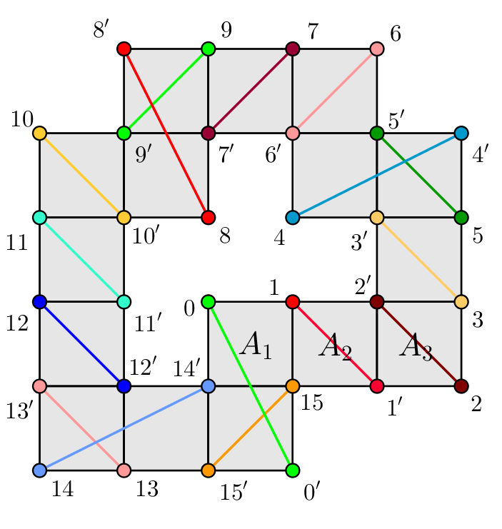
Figure 18.

Proposition 4.7.

Let $\mathcal{P}:A_{1},\dots,A_{n}$ be a closed path polyomino. Suppose that $\mathcal{P}$ has an $L$-configuration in every change of direction. Consider such an $L$-configuration as in Figure 19 (A), up to relabelling of the cells of $\mathcal{P}$. Then $I_{\mathcal{P}}$ is of Kőnig type.

Proof.

We distinguish three cases depending on the position of $A_{4}$ with respect to $A_{3}$. First of all, we assume that $A_{4}$ is at North of $A_{3}$. We set $Y^{(1)}=Y^{(1)}_{1}\sqcup Y^{(1)}_{2}$ where $Y^{(1)}_{1}=\{x_{1},x_{2}\}$ and $Y^{(1)}_{2}=\{x_{1^{\prime}},x_{2^{\prime}}\}$ with $x_{1}>x_{2}>x_{1^{\prime}}>x_{2^{\prime}}$, with reference to Figure 19 (A). The procedure described in Definition 4.3 finishes with one of the two cases displayed in Figure 19 (B) and (C). As done in Proposition 4.4 the desired conclusion follows.

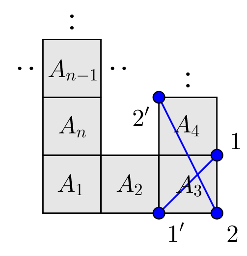
(a)

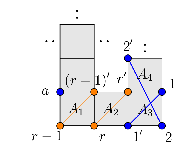
(b) Note $a\in Y_{2}$

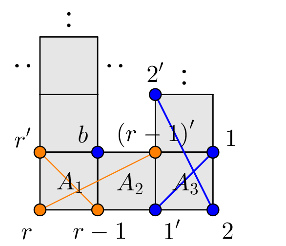
(c) Note $b\in Y_{2}$

Figure 19.

We assume that $A_{4}$ is at South of $A_{3}$. In such a case we set $Y^{(1)}=Y^{(1)}_{1}\sqcup Y^{(1)}_{2}$ where $Y^{(1)}_{1}=\{x_{1}\}$ and $Y^{(1)}_{2}=\{x_{1^{\prime}}\}$ with $x_{1}>x_{1^{\prime}}$, with reference to Figure 20 (A). Observe that the only two last cases are in Figure 20 (B) and (C).

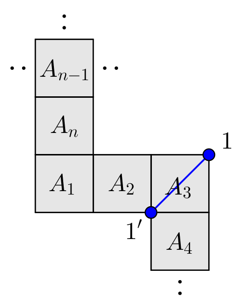
(a)

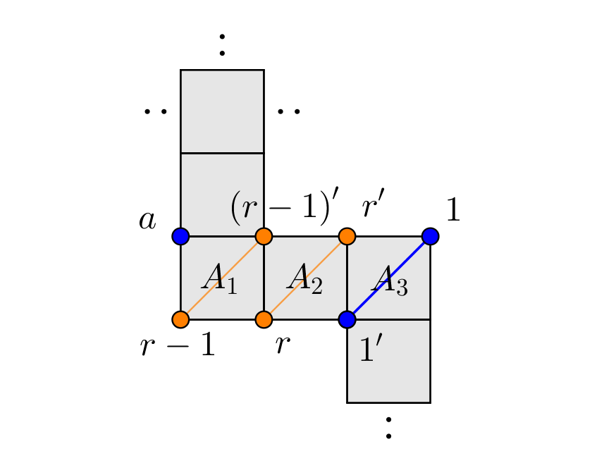
(b) Note $a\in Y_{2}$

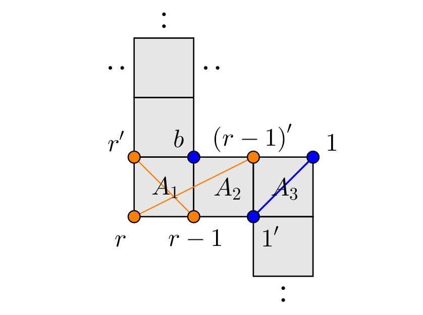
(c) Note $b\in Y_{2}$

Figure 20.

We assume that $A_{4}$ is at East of $A_{3}$. In such a case we set $Y^{(1)}=Y^{(1)}_{1}\sqcup Y^{(1)}_{2}$ where $Y^{(1)}_{1}=\{x_{3}\}$ and $Y^{(1)}_{2}=\{x_{3^{\prime}}\}$ with $x_{3}>x_{3^{\prime}}$, with reference to Figure 21 (A). Observe that the only two last cases are in Figure 21 (B) and (C), where we set:

$$x_{1}>x_{2}>x_{3}\dots>x_{r}>x_{1^{\prime}}>x_{2^{\prime}}>x_{3^{\prime}}\dots>x_{r^{\prime}}.$$

The conclusion follows arguing as before.

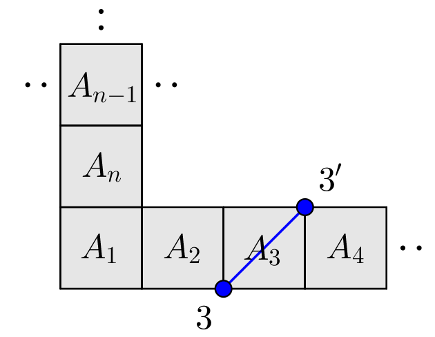
(a)

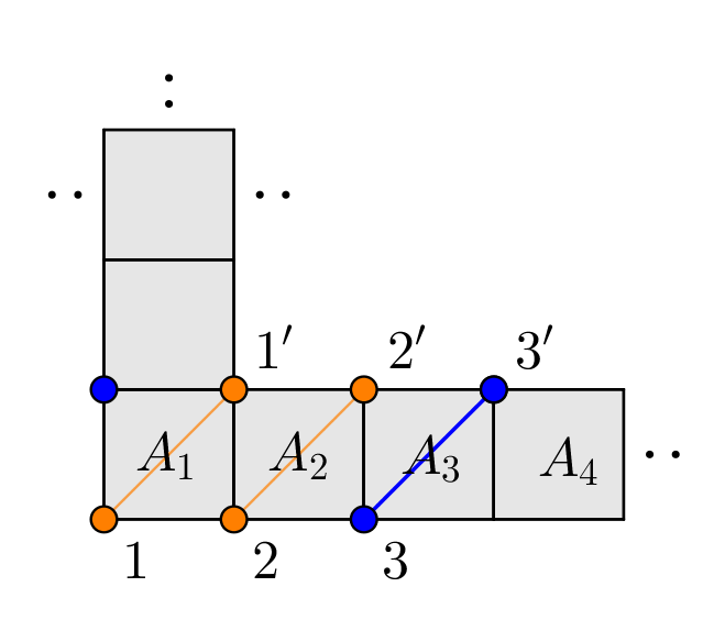
(b)

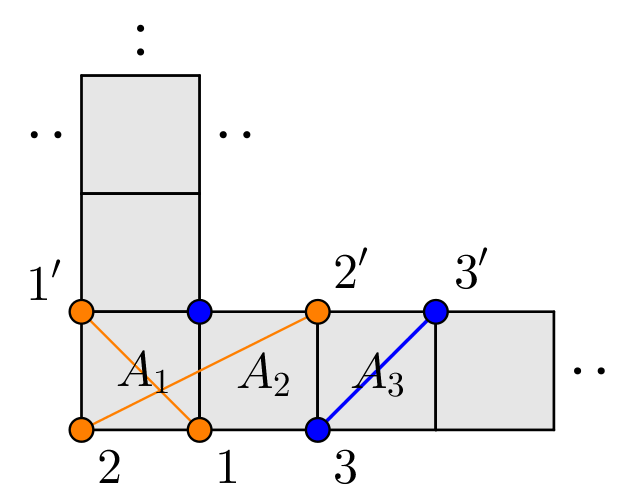
(c)

Figure 21.

∎

Example 4.8.

In Figure 22 we show two examples of the procedure described in Proposition 4.4. In particular, $\mathcal{P}_{1}$ is of Kőnig type with respect the lexicographic order induced by

$$x_{1}>x_{2}>\dots>x_{26}>x_{1^{\prime}}>x_{2^{\prime}}>\dots>x_{26^{\prime}}$$

and to the sixty generators of $I_{\mathcal{P}_{1}}$ corresponding to the inner intervals having $i$ and $i^{\prime}$ as diagonal or anti-diagonal corners, for all $i\in[26]$; as well as for the polyomino $\mathcal{P}_{2}$ similarly.

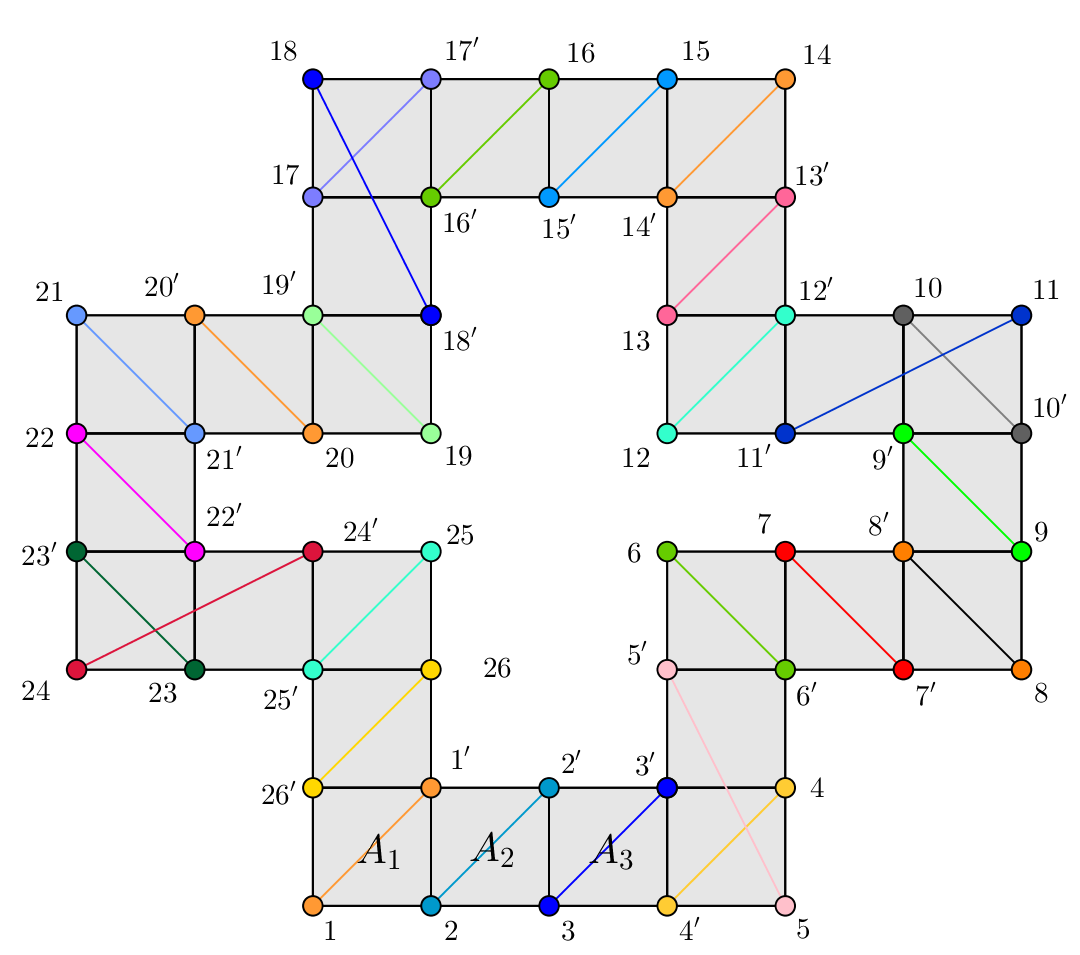
(a) Closed path $\mathcal{P}_{1}$

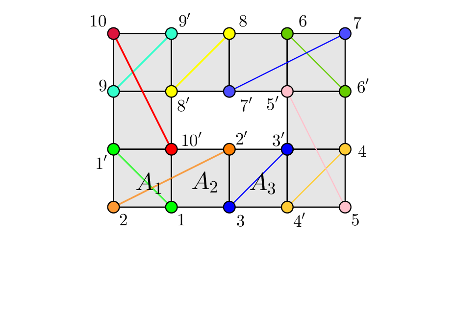
(b) Closed path $\mathcal{P}_{2}$

Figure 22.

Theorem 4.9.

Let $\mathcal{P}$ be a closed path polyomino. Then $I_{\mathcal{P}}$ is of Kőnig type.

Proof.

If $\mathcal{P}$ contains a configuration of four cells as in Figure 14 (A), then $I_{\mathcal{P}}$ is of Kőnig type by Proposition 4.4. If $\mathcal{P}$ does not contain any such configuration, then it is easy to see that $\mathcal{P}$ has an $L$-configuration in every change of direction, so $I_{\mathcal{P}}$ is of Kőnig type by Proposition 4.7. Hence, the desired claim is proved. ∎

5. A combinatorial interpretation of the canonical module

As an application of the Kőnig type property, in this section we present a sub-class of closed path polyominoes, for which the canonical module has a very nice combinatorial description; refer to [2, Section 3.3] for more details on the canonical module of a Cohen-Macaulay ring. Let us start by introducing some definitions and notations.

Definition 5.1.

Let $I_{1}=[(1,1),(m,n)]$ and $I_{2}=[(2,2),(m-1,n-1)]$, where $m,n\geq 4$ and $(m,n)\neq(4,4)$. We say that a closed path $\mathcal{P}$ is a circle if $\mathcal{P}=\mathcal{P}_{I_{1}}\setminus\mathcal{P}_{I_{2}}$.

We require that $m$ and $n$ are not equal to four at the same time, because in such a case $\mathcal{P}$ consists of maximal blocks of length three so $K[\mathcal{P}]$ is Gorenstein by [8, Theorem 5.7] and we know that the canonical module of $K[\mathcal{P}]$ is isomorphic to $K[\mathcal{P}]$ (see [2, Theorem 3.3.7].

In the description of the canonical module of a circle closed path, the binomial ideal coming from the Kőnig type property and a suitable monomial ideal will play a crucial role. We set the following.

Definition 5.2.

We introduce two ideals to describe the canonical module of a circle closed path.
Let $\mathcal{P}$ be a closed path. With reference to Proposition 4.7, we denote by $J(\mathcal{P})$ the binomial ideal generated by the generators of $I_{\mathcal{P}}$ corresponding to the inner intervals of $\mathcal{P}$ having $i$ and $i^{\prime}$ as diagonal or anti-diagonal corners, for all $i\in[\mathrm{rank}(\mathcal{P})]$.
Now, let $\mathcal{P}$ be a circle closed path. We introduce the following sets of vertices of $\mathcal{P}$. Let $m,n>4$.

• $L_{j-2}=\{(1,j),(2,j)\}$ and $R_{j-2}=\{(m-1,j),(m,j)\}$ for all $j\in[n-2]\setminus\{1,2\}$;

• $U_{k-2}=\{(k,n),(k,n-1)\}$ and $D_{k-2}=\{(k,1),(k,2)\}$ for all $k\in[m-2]\setminus\{1,2\}$.

In addition, we set the following Cartesian product.

1. If $m,n>4$, then

   $$C=\Bigg{(}\bigtimes_{i=1}^{n-4}L_{i}\Bigg{)}\times\Bigg{(}\bigtimes_{i=1}^{n-4}R_{i}\Bigg{)}\times\Bigg{(}\bigtimes_{i=1}^{m-4}U_{i}\Bigg{)}\times\Bigg{(}\bigtimes_{i=1}^{m-4}D_{i}\Bigg{)}.$$

   Set $t=2(n+m-8)$ in such a case.

2. If $m>4$ and $n=4$, then

   $$C=\Bigg{(}\bigtimes_{i=1}^{m-4}U_{i}\Bigg{)}\times\Bigg{(}\bigtimes_{i=1}^{m-4}D_{i}\Bigg{)}.$$

   Let $t=2(m-4)$ in this case.

3. If $m=4$ and $n>4$, then

   $$C=\Bigg{(}\bigtimes_{i=1}^{n-4}L_{i}\Bigg{)}\times\Bigg{(}\bigtimes_{i=1}^{n-4}R_{i}\Bigg{)}.$$

   Set $t=2(n-4)$ here.

Now, we define a suitable subset of $C$.

$$\mathcal{V}=\big{\{}(v_{1},\dots,v_{t})\in C:v_{i},v_{j}\text{ are not the diagonal corners of an inner interval of }\mathcal{P},\text{ for }i,j\in[t]\big{\}}.$$

For all $\mathbf{v}=(v_{1},\dots,v_{t})\in\mathcal{V}$, we define a monomial in $S_{\mathcal{P}}$ as

$$\mathbf{x}_{\mathbf{v}}=x_{v_{1}}x_{v_{2}}\dots x_{v_{t}}x_{(2,2)}x_{(1,n)}x_{(m,1)}x_{(m-1,n-1)},$$

and we denote by $K(\mathcal{P})$ the monomial ideal in $S_{\mathcal{P}}$ generated by $\mathbf{x}_{\mathbf{v}}$ for all $\mathbf{v}\in\mathcal{V}.$

Remark 5.3.

Let $\mathcal{P}$ be a circle closed path and $K(\mathcal{P})$ be the ideal defined in Definition 5.2. Observe that $K(\mathcal{P})$ is a squarefree monomial ideal generated in degree $t+4$. In addition, let us denote by $\mu(K(\mathcal{P}))$ the number of monomial generators of $K(\mathcal{P})$. We have that:

$$\mu(K(\mathcal{P}))=\left\{\begin{array}[]{ll}(m-3)^{2}(n-3)^{2},&m,n>4;\\ (n-3)^{2},&m=4,n>4;\\ (m-3)^{2},&m>4,n=4.\\ \end{array}\right.$$

We will assume that $m,n>4$. Consider $L=L_{1}\times\dots\times L_{n-4}$ and $w_{0}=\big{(}(1,3),(1,4),\dots,(1,m-2)\big{)}\in L.$ All the other $(m-4)$-uple of $L$, where the vertices are not the diagonal corners of an inner interval of $\mathcal{P}$, can be obtained replacing in $w_{i}$ in the $i$-th component $(i,1)$ with $(i,2)$, for all $i\in[m-4]$. Hence, the number of such configurations is $m-3$. As a consequence of the symmetric structure of $\mathcal{P}$, we have that $\mu(K(\mathcal{P}))=(m-3)^{2}(n-3)^{2}$. The same arguments hold in the other two cases.

We state now the main theorem of this section:

Theorem 5.4.

Let $\mathcal{P}$ be a circle closed path. We denote by $\omega_{K[\mathcal{P}]}$ the canonical module of $K[\mathcal{P}]$. Then:

$$\omega_{K[\mathcal{P}]}\cong{\raisebox{1.99997pt}{$(J(\mathcal{P})+K(\mathcal{P}))$}\left/\raisebox{-1.99997pt}{$J(\mathcal{P})$}\right.}$$

where $J(\mathcal{P})$ and $K(\mathcal{P})$ are the ideals given in Definition 5.2.

Before proving Theorem 5.4, we provide an example to figure out the combinatorial description of the canonical module of $K[\mathcal{P}]$.

Example 5.5.

Let $\mathcal{P}$ be the circle closed path as in Figure 23.

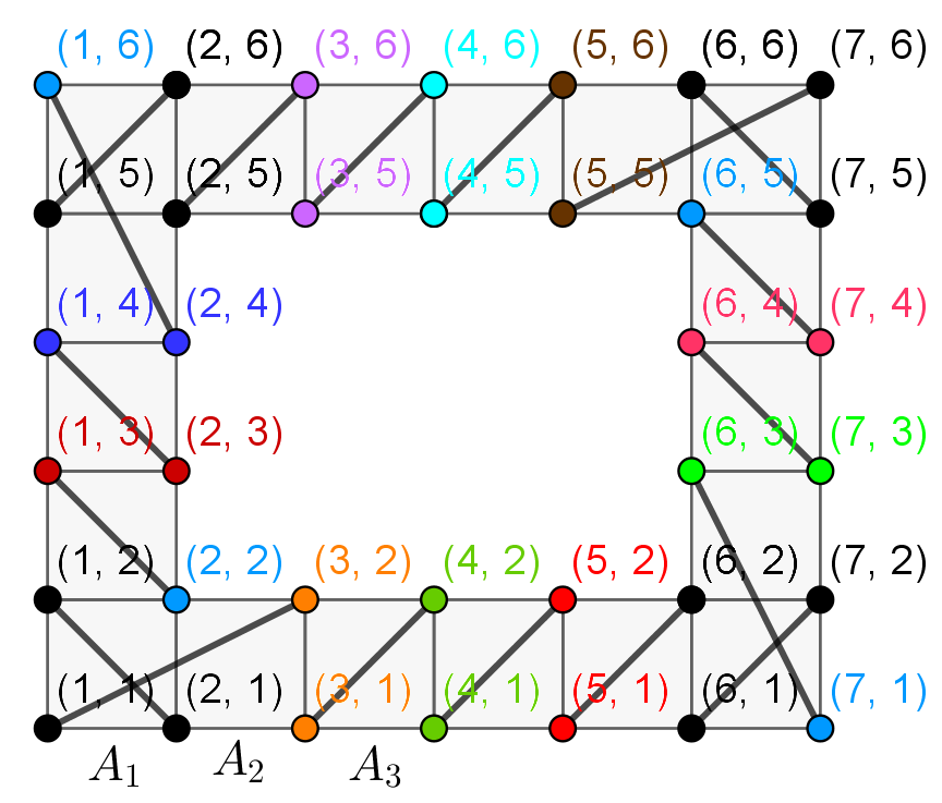
Figure 23.

By Proposition 4.7, the ideal $J(\mathcal{P})$ is generated by the binomials:

$$x_{6,5}x_{7,6}-x_{6,6}x_{7,5},\,x_{6,4}x_{7,5}-x_{6,5}x_{7,4},\,x_{6,3}x_{7,4}-x_{6,4}x_{7,3},\,x_{6,1}x_{7,3}-x_{6,3}x_{7,1},\,x_{6,1}x_{7,2}-x_{6,2}x_{7,1},\,$$

$$x_{5,5}x_{7,6}-x_{5,6}x_{7,5},\,x_{5,1}x_{6,2}-x_{5,2}x_{6,1},\,x_{4,5}x_{5,6}-x_{4,6}x_{5,5},\,x_{4,1}x_{5,2}-x_{4,2}x_{5,1},\,x_{3,5}x_{4,6}-x_{3,6}x_{4,5},\,$$

$$x_{3,1}x_{4,2}-x_{3,2}x_{4,1},\,x_{2,5}x_{3,6}-x_{2,6}x_{3,5},\,x_{1,5}x_{2,6}-x_{1,6}x_{2,5},\,x_{1,4}x_{2,6}-x_{1,6}x_{2,4},\,x_{1,3}x_{2,4}-x_{1,4}x_{2,3},\,$$

$$x_{1,2}x_{2,3}-x_{1,3}x_{2,2},\,x_{1,1}x_{3,2}-x_{1,2}x_{3,1},\,x_{1,1}x_{2,2}-x_{1,2}x_{2,1}.$$

Since $m=6$ and $n=5$, we have that $t=14$ and $\mu(K(\mathcal{P}))=144$. The ideal $K(\mathcal{P})$ is generated by the following $144$ monomials in degree $14$:

$$x_{1,6}x_{2,2}x_{2,3}x_{2,4}x_{3,2}x_{3,6}x_{4,2}x_{4,6}x_{5,2}x_{5,6}x_{6,5}x_{7,1}x_{7,3}x_{7,4},\,x_{1,6}x_{2,2}x_{2,3}x_{2,4}x_{3,2}x_{3,6}x_{4,2}x_{4,6}x_{5,2}x_{5,6}x_{6,4}x_{6,5}x_{7,1}x_{7,3},\,$$

$$x_{1,6}x_{2,2}x_{2,3}x_{2,4}x_{3,2}x_{3,6}x_{4,2}x_{4,6}x_{5,2}x_{5,6}x_{6,3}x_{6,4}x_{6,5}x_{7,1},\,x_{1,6}x_{2,2}x_{2,3}x_{2,4}x_{3,2}x_{3,6}x_{4,2}x_{4,6}x_{5,2}x_{5,5}x_{6,5}x_{7,1}x_{7,3}x_{7,4},\,$$

$$x_{1,6}x_{2,2}x_{2,3}x_{2,4}x_{3,2}x_{3,6}x_{4,2}x_{4,6}x_{5,2}x_{5,5}x_{6,4}x_{6,5}x_{7,1}x_{7,3},\,x_{1,6}x_{2,2}x_{2,3}x_{2,4}x_{3,2}x_{3,6}x_{4,2}x_{4,6}x_{5,2}x_{5,5}x_{6,3}x_{6,4}x_{6,5}x_{7,1},\,$$

$$x_{1,6}x_{2,2}x_{2,3}x_{2,4}x_{3,2}x_{3,6}x_{4,2}x_{4,6}x_{5,1}x_{5,6}x_{6,5}x_{7,1}x_{7,3}x_{7,4},\,x_{1,6}x_{2,2}x_{2,3}x_{2,4}x_{3,2}x_{3,6}x_{4,2}x_{4,6}x_{5,1}x_{5,6}x_{6,4}x_{6,5}x_{7,1}x_{7,3},\,$$

$$x_{1,6}x_{2,2}x_{2,3}x_{2,4}x_{3,2}x_{3,6}x_{4,2}x_{4,6}x_{5,1}x_{5,6}x_{6,3}x_{6,4}x_{6,5}x_{7,1},\,x_{1,6}x_{2,2}x_{2,3}x_{2,4}x_{3,2}x_{3,6}x_{4,2}x_{4,6}x_{5,1}x_{5,5}x_{6,5}x_{7,1}x_{7,3}x_{7,4},\,$$

$$x_{1,6}x_{2,2}x_{2,3}x_{2,4}x_{3,2}x_{3,6}x_{4,2}x_{4,6}x_{5,1}x_{5,5}x_{6,4}x_{6,5}x_{7,1}x_{7,3},\,x_{1,6}x_{2,2}x_{2,3}x_{2,4}x_{3,2}x_{3,6}x_{4,2}x_{4,6}x_{5,1}x_{5,5}x_{6,3}x_{6,4}x_{6,5}x_{7,1},\,$$

$$x_{1,6}x_{2,2}x_{2,3}x_{2,4}x_{3,2}x_{3,6}x_{4,2}x_{4,5}x_{5,2}x_{5,5}x_{6,5}x_{7,1}x_{7,3}x_{7,4},\,x_{1,6}x_{2,2}x_{2,3}x_{2,4}x_{3,2}x_{3,6}x_{4,2}x_{4,5}x_{5,2}x_{5,5}x_{6,4}x_{6,5}x_{7,1}x_{7,3},\,$$

$$x_{1,6}x_{2,2}x_{2,3}x_{2,4}x_{3,2}x_{3,6}x_{4,2}x_{4,5}x_{5,2}x_{5,5}x_{6,3}x_{6,4}x_{6,5}x_{7,1},\,x_{1,6}x_{2,2}x_{2,3}x_{2,4}x_{3,2}x_{3,6}x_{4,2}x_{4,5}x_{5,1}x_{5,5}x_{6,5}x_{7,1}x_{7,3}x_{7,4},\,$$

$$x_{1,6}x_{2,2}x_{2,3}x_{2,4}x_{3,2}x_{3,6}x_{4,2}x_{4,5}x_{5,1}x_{5,5}x_{6,4}x_{6,5}x_{7,1}x_{7,3},\,x_{1,6}x_{2,2}x_{2,3}x_{2,4}x_{3,2}x_{3,6}x_{4,2}x_{4,5}x_{5,1}x_{5,5}x_{6,3}x_{6,4}x_{6,5}x_{7,1},\,$$

$$x_{1,6}x_{2,2}x_{2,3}x_{2,4}x_{3,2}x_{3,6}x_{4,1}x_{4,6}x_{5,1}x_{5,6}x_{6,5}x_{7,1}x_{7,3}x_{7,4},\,x_{1,6}x_{2,2}x_{2,3}x_{2,4}x_{3,2}x_{3,6}x_{4,1}x_{4,6}x_{5,1}x_{5,6}x_{6,4}x_{6,5}x_{7,1}x_{7,3},\,$$

$$x_{1,6}x_{2,2}x_{2,3}x_{2,4}x_{3,2}x_{3,6}x_{4,1}x_{4,6}x_{5,1}x_{5,6}x_{6,3}x_{6,4}x_{6,5}x_{7,1},\,x_{1,6}x_{2,2}x_{2,3}x_{2,4}x_{3,2}x_{3,6}x_{4,1}x_{4,6}x_{5,1}x_{5,5}x_{6,5}x_{7,1}x_{7,3}x_{7,4},\,$$

$$x_{1,6}x_{2,2}x_{2,3}x_{2,4}x_{3,2}x_{3,6}x_{4,1}x_{4,6}x_{5,1}x_{5,5}x_{6,4}x_{6,5}x_{7,1}x_{7,3},\,x_{1,6}x_{2,2}x_{2,3}x_{2,4}x_{3,2}x_{3,6}x_{4,1}x_{4,6}x_{5,1}x_{5,5}x_{6,3}x_{6,4}x_{6,5}x_{7,1},\,$$

$$x_{1,6}x_{2,2}x_{2,3}x_{2,4}x_{3,2}x_{3,6}x_{4,1}x_{4,5}x_{5,1}x_{5,5}x_{6,5}x_{7,1}x_{7,3}x_{7,4},\,x_{1,6}x_{2,2}x_{2,3}x_{2,4}x_{3,2}x_{3,6}x_{4,1}x_{4,5}x_{5,1}x_{5,5}x_{6,4}x_{6,5}x_{7,1}x_{7,3},\,$$

$$x_{1,6}x_{2,2}x_{2,3}x_{2,4}x_{3,2}x_{3,6}x_{4,1}x_{4,5}x_{5,1}x_{5,5}x_{6,3}x_{6,4}x_{6,5}x_{7,1},\,x_{1,6}x_{2,2}x_{2,3}x_{2,4}x_{3,2}x_{3,5}x_{4,2}x_{4,5}x_{5,2}x_{5,5}x_{6,5}x_{7,1}x_{7,3}x_{7,4},\,$$

$$x_{1,6}x_{2,2}x_{2,3}x_{2,4}x_{3,2}x_{3,5}x_{4,2}x_{4,5}x_{5,2}x_{5,5}x_{6,4}x_{6,5}x_{7,1}x_{7,3},\,x_{1,6}x_{2,2}x_{2,3}x_{2,4}x_{3,2}x_{3,5}x_{4,2}x_{4,5}x_{5,2}x_{5,5}x_{6,3}x_{6,4}x_{6,5}x_{7,1},\,$$

$$x_{1,6}x_{2,2}x_{2,3}x_{2,4}x_{3,2}x_{3,5}x_{4,2}x_{4,5}x_{5,1}x_{5,5}x_{6,5}x_{7,1}x_{7,3}x_{7,4},\,x_{1,6}x_{2,2}x_{2,3}x_{2,4}x_{3,2}x_{3,5}x_{4,2}x_{4,5}x_{5,1}x_{5,5}x_{6,4}x_{6,5}x_{7,1}x_{7,3},\,$$

$$x_{1,6}x_{2,2}x_{2,3}x_{2,4}x_{3,2}x_{3,5}x_{4,2}x_{4,5}x_{5,1}x_{5,5}x_{6,3}x_{6,4}x_{6,5}x_{7,1},\,x_{1,6}x_{2,2}x_{2,3}x_{2,4}x_{3,2}x_{3,5}x_{4,1}x_{4,5}x_{5,1}x_{5,5}x_{6,5}x_{7,1}x_{7,3}x_{7,4},\,$$

$$x_{1,6}x_{2,2}x_{2,3}x_{2,4}x_{3,2}x_{3,5}x_{4,1}x_{4,5}x_{5,1}x_{5,5}x_{6,4}x_{6,5}x_{7,1}x_{7,3},\,x_{1,6}x_{2,2}x_{2,3}x_{2,4}x_{3,2}x_{3,5}x_{4,1}x_{4,5}x_{5,1}x_{5,5}x_{6,3}x_{6,4}x_{6,5}x_{7,1},\,$$

$$x_{1,6}x_{2,2}x_{2,3}x_{2,4}x_{3,1}x_{3,6}x_{4,1}x_{4,6}x_{5,1}x_{5,6}x_{6,5}x_{7,1}x_{7,3}x_{7,4},\,x_{1,6}x_{2,2}x_{2,3}x_{2,4}x_{3,1}x_{3,6}x_{4,1}x_{4,6}x_{5,1}x_{5,6}x_{6,4}x_{6,5}x_{7,1}x_{7,3},\,$$

$$x_{1,6}x_{2,2}x_{2,3}x_{2,4}x_{3,1}x_{3,6}x_{4,1}x_{4,6}x_{5,1}x_{5,6}x_{6,3}x_{6,4}x_{6,5}x_{7,1},\,x_{1,6}x_{2,2}x_{2,3}x_{2,4}x_{3,1}x_{3,6}x_{4,1}x_{4,6}x_{5,1}x_{5,5}x_{6,5}x_{7,1}x_{7,3}x_{7,4},\,$$

$$x_{1,6}x_{2,2}x_{2,3}x_{2,4}x_{3,1}x_{3,6}x_{4,1}x_{4,6}x_{5,1}x_{5,5}x_{6,4}x_{6,5}x_{7,1}x_{7,3},\,x_{1,6}x_{2,2}x_{2,3}x_{2,4}x_{3,1}x_{3,6}x_{4,1}x_{4,6}x_{5,1}x_{5,5}x_{6,3}x_{6,4}x_{6,5}x_{7,1},\,$$

$$x_{1,6}x_{2,2}x_{2,3}x_{2,4}x_{3,1}x_{3,6}x_{4,1}x_{4,5}x_{5,1}x_{5,5}x_{6,5}x_{7,1}x_{7,3}x_{7,4},\,x_{1,6}x_{2,2}x_{2,3}x_{2,4}x_{3,1}x_{3,6}x_{4,1}x_{4,5}x_{5,1}x_{5,5}x_{6,4}x_{6,5}x_{7,1}x_{7,3},\,$$

$$x_{1,6}x_{2,2}x_{2,3}x_{2,4}x_{3,1}x_{3,6}x_{4,1}x_{4,5}x_{5,1}x_{5,5}x_{6,3}x_{6,4}x_{6,5}x_{7,1},\,x_{1,6}x_{2,2}x_{2,3}x_{2,4}x_{3,1}x_{3,5}x_{4,1}x_{4,5}x_{5,1}x_{5,5}x_{6,5}x_{7,1}x_{7,3}x_{7,4},\,$$

$$x_{1,6}x_{2,2}x_{2,3}x_{2,4}x_{3,1}x_{3,5}x_{4,1}x_{4,5}x_{5,1}x_{5,5}x_{6,4}x_{6,5}x_{7,1}x_{7,3},\,x_{1,6}x_{2,2}x_{2,3}x_{2,4}x_{3,1}x_{3,5}x_{4,1}x_{4,5}x_{5,1}x_{5,5}x_{6,3}x_{6,4}x_{6,5}x_{7,1},\,$$

$$x_{1,4}x_{1,6}x_{2,2}x_{2,3}x_{3,2}x_{3,6}x_{4,2}x_{4,6}x_{5,2}x_{5,6}x_{6,5}x_{7,1}x_{7,3}x_{7,4},\,x_{1,4}x_{1,6}x_{2,2}x_{2,3}x_{3,2}x_{3,6}x_{4,2}x_{4,6}x_{5,2}x_{5,6}x_{6,4}x_{6,5}x_{7,1}x_{7,3},\,$$

$$x_{1,4}x_{1,6}x_{2,2}x_{2,3}x_{3,2}x_{3,6}x_{4,2}x_{4,6}x_{5,2}x_{5,6}x_{6,3}x_{6,4}x_{6,5}x_{7,1},\,x_{1,4}x_{1,6}x_{2,2}x_{2,3}x_{3,2}x_{3,6}x_{4,2}x_{4,6}x_{5,2}x_{5,5}x_{6,5}x_{7,1}x_{7,3}x_{7,4},\,$$

$$x_{1,4}x_{1,6}x_{2,2}x_{2,3}x_{3,2}x_{3,6}x_{4,2}x_{4,6}x_{5,2}x_{5,5}x_{6,4}x_{6,5}x_{7,1}x_{7,3},\,x_{1,4}x_{1,6}x_{2,2}x_{2,3}x_{3,2}x_{3,6}x_{4,2}x_{4,6}x_{5,2}x_{5,5}x_{6,3}x_{6,4}x_{6,5}x_{7,1},\,$$

$$x_{1,4}x_{1,6}x_{2,2}x_{2,3}x_{3,2}x_{3,6}x_{4,2}x_{4,6}x_{5,1}x_{5,6}x_{6,5}x_{7,1}x_{7,3}x_{7,4},\,x_{1,4}x_{1,6}x_{2,2}x_{2,3}x_{3,2}x_{3,6}x_{4,2}x_{4,6}x_{5,1}x_{5,6}x_{6,4}x_{6,5}x_{7,1}x_{7,3},\,$$

$$x_{1,4}x_{1,6}x_{2,2}x_{2,3}x_{3,2}x_{3,6}x_{4,2}x_{4,6}x_{5,1}x_{5,6}x_{6,3}x_{6,4}x_{6,5}x_{7,1},\,x_{1,4}x_{1,6}x_{2,2}x_{2,3}x_{3,2}x_{3,6}x_{4,2}x_{4,6}x_{5,1}x_{5,5}x_{6,5}x_{7,1}x_{7,3}x_{7,4},\,$$

$$x_{1,4}x_{1,6}x_{2,2}x_{2,3}x_{3,2}x_{3,6}x_{4,2}x_{4,6}x_{5,1}x_{5,5}x_{6,4}x_{6,5}x_{7,1}x_{7,3},\,x_{1,4}x_{1,6}x_{2,2}x_{2,3}x_{3,2}x_{3,6}x_{4,2}x_{4,6}x_{5,1}x_{5,5}x_{6,3}x_{6,4}x_{6,5}x_{7,1},\,$$

$$x_{1,4}x_{1,6}x_{2,2}x_{2,3}x_{3,2}x_{3,6}x_{4,2}x_{4,5}x_{5,2}x_{5,5}x_{6,5}x_{7,1}x_{7,3}x_{7,4},\,x_{1,4}x_{1,6}x_{2,2}x_{2,3}x_{3,2}x_{3,6}x_{4,2}x_{4,5}x_{5,2}x_{5,5}x_{6,4}x_{6,5}x_{7,1}x_{7,3},\,$$

$$x_{1,4}x_{1,6}x_{2,2}x_{2,3}x_{3,2}x_{3,6}x_{4,2}x_{4,5}x_{5,2}x_{5,5}x_{6,3}x_{6,4}x_{6,5}x_{7,1},\,x_{1,4}x_{1,6}x_{2,2}x_{2,3}x_{3,2}x_{3,6}x_{4,2}x_{4,5}x_{5,1}x_{5,5}x_{6,5}x_{7,1}x_{7,3}x_{7,4},\,$$

$$x_{1,4}x_{1,6}x_{2,2}x_{2,3}x_{3,2}x_{3,6}x_{4,2}x_{4,5}x_{5,1}x_{5,5}x_{6,4}x_{6,5}x_{7,1}x_{7,3},\,x_{1,4}x_{1,6}x_{2,2}x_{2,3}x_{3,2}x_{3,6}x_{4,2}x_{4,5}x_{5,1}x_{5,5}x_{6,3}x_{6,4}x_{6,5}x_{7,1},\,$$

$$x_{1,4}x_{1,6}x_{2,2}x_{2,3}x_{3,2}x_{3,6}x_{4,1}x_{4,6}x_{5,1}x_{5,6}x_{6,5}x_{7,1}x_{7,3}x_{7,4},\,x_{1,4}x_{1,6}x_{2,2}x_{2,3}x_{3,2}x_{3,6}x_{4,1}x_{4,6}x_{5,1}x_{5,6}x_{6,4}x_{6,5}x_{7,1}x_{7,3},\,$$

$$x_{1,4}x_{1,6}x_{2,2}x_{2,3}x_{3,2}x_{3,6}x_{4,1}x_{4,6}x_{5,1}x_{5,6}x_{6,3}x_{6,4}x_{6,5}x_{7,1},\,x_{1,4}x_{1,6}x_{2,2}x_{2,3}x_{3,2}x_{3,6}x_{4,1}x_{4,6}x_{5,1}x_{5,5}x_{6,5}x_{7,1}x_{7,3}x_{7,4},\,$$

$$x_{1,4}x_{1,6}x_{2,2}x_{2,3}x_{3,2}x_{3,6}x_{4,1}x_{4,6}x_{5,1}x_{5,5}x_{6,4}x_{6,5}x_{7,1}x_{7,3},\,x_{1,4}x_{1,6}x_{2,2}x_{2,3}x_{3,2}x_{3,6}x_{4,1}x_{4,6}x_{5,1}x_{5,5}x_{6,3}x_{6,4}x_{6,5}x_{7,1},\,$$

$$x_{1,4}x_{1,6}x_{2,2}x_{2,3}x_{3,2}x_{3,6}x_{4,1}x_{4,5}x_{5,1}x_{5,5}x_{6,5}x_{7,1}x_{7,3}x_{7,4},\,x_{1,4}x_{1,6}x_{2,2}x_{2,3}x_{3,2}x_{3,6}x_{4,1}x_{4,5}x_{5,1}x_{5,5}x_{6,4}x_{6,5}x_{7,1}x_{7,3},\,$$

$$x_{1,4}x_{1,6}x_{2,2}x_{2,3}x_{3,2}x_{3,6}x_{4,1}x_{4,5}x_{5,1}x_{5,5}x_{6,3}x_{6,4}x_{6,5}x_{7,1},\,x_{1,4}x_{1,6}x_{2,2}x_{2,3}x_{3,2}x_{3,5}x_{4,2}x_{4,5}x_{5,2}x_{5,5}x_{6,5}x_{7,1}x_{7,3}x_{7,4},\,$$

$$x_{1,4}x_{1,6}x_{2,2}x_{2,3}x_{3,2}x_{3,5}x_{4,2}x_{4,5}x_{5,2}x_{5,5}x_{6,4}x_{6,5}x_{7,1}x_{7,3},\,x_{1,4}x_{1,6}x_{2,2}x_{2,3}x_{3,2}x_{3,5}x_{4,2}x_{4,5}x_{5,2}x_{5,5}x_{6,3}x_{6,4}x_{6,5}x_{7,1},\,$$

$$x_{1,4}x_{1,6}x_{2,2}x_{2,3}x_{3,2}x_{3,5}x_{4,2}x_{4,5}x_{5,1}x_{5,5}x_{6,5}x_{7,1}x_{7,3}x_{7,4},\,x_{1,4}x_{1,6}x_{2,2}x_{2,3}x_{3,2}x_{3,5}x_{4,2}x_{4,5}x_{5,1}x_{5,5}x_{6,4}x_{6,5}x_{7,1}x_{7,3},\,$$

$$x_{1,4}x_{1,6}x_{2,2}x_{2,3}x_{3,2}x_{3,5}x_{4,2}x_{4,5}x_{5,1}x_{5,5}x_{6,3}x_{6,4}x_{6,5}x_{7,1},\,x_{1,4}x_{1,6}x_{2,2}x_{2,3}x_{3,2}x_{3,5}x_{4,1}x_{4,5}x_{5,1}x_{5,5}x_{6,5}x_{7,1}x_{7,3}x_{7,4},\,$$

$$x_{1,4}x_{1,6}x_{2,2}x_{2,3}x_{3,2}x_{3,5}x_{4,1}x_{4,5}x_{5,1}x_{5,5}x_{6,4}x_{6,5}x_{7,1}x_{7,3},\,x_{1,4}x_{1,6}x_{2,2}x_{2,3}x_{3,2}x_{3,5}x_{4,1}x_{4,5}x_{5,1}x_{5,5}x_{6,3}x_{6,4}x_{6,5}x_{7,1},\,$$

$$x_{1,4}x_{1,6}x_{2,2}x_{2,3}x_{3,1}x_{3,6}x_{4,1}x_{4,6}x_{5,1}x_{5,6}x_{6,5}x_{7,1}x_{7,3}x_{7,4},\,x_{1,4}x_{1,6}x_{2,2}x_{2,3}x_{3,1}x_{3,6}x_{4,1}x_{4,6}x_{5,1}x_{5,6}x_{6,4}x_{6,5}x_{7,1}x_{7,3},\,$$

$$x_{1,4}x_{1,6}x_{2,2}x_{2,3}x_{3,1}x_{3,6}x_{4,1}x_{4,6}x_{5,1}x_{5,6}x_{6,3}x_{6,4}x_{6,5}x_{7,1},\,x_{1,4}x_{1,6}x_{2,2}x_{2,3}x_{3,1}x_{3,6}x_{4,1}x_{4,6}x_{5,1}x_{5,5}x_{6,5}x_{7,1}x_{7,3}x_{7,4},\,$$

$$x_{1,4}x_{1,6}x_{2,2}x_{2,3}x_{3,1}x_{3,6}x_{4,1}x_{4,6}x_{5,1}x_{5,5}x_{6,4}x_{6,5}x_{7,1}x_{7,3},\,x_{1,4}x_{1,6}x_{2,2}x_{2,3}x_{3,1}x_{3,6}x_{4,1}x_{4,6}x_{5,1}x_{5,5}x_{6,3}x_{6,4}x_{6,5}x_{7,1},\,$$

$$x_{1,4}x_{1,6}x_{2,2}x_{2,3}x_{3,1}x_{3,6}x_{4,1}x_{4,5}x_{5,1}x_{5,5}x_{6,5}x_{7,1}x_{7,3}x_{7,4},\,x_{1,4}x_{1,6}x_{2,2}x_{2,3}x_{3,1}x_{3,6}x_{4,1}x_{4,5}x_{5,1}x_{5,5}x_{6,4}x_{6,5}x_{7,1}x_{7,3},\,$$

$$x_{1,4}x_{1,6}x_{2,2}x_{2,3}x_{3,1}x_{3,6}x_{4,1}x_{4,5}x_{5,1}x_{5,5}x_{6,3}x_{6,4}x_{6,5}x_{7,1},\,x_{1,4}x_{1,6}x_{2,2}x_{2,3}x_{3,1}x_{3,5}x_{4,1}x_{4,5}x_{5,1}x_{5,5}x_{6,5}x_{7,1}x_{7,3}x_{7,4},\,$$

$$x_{1,4}x_{1,6}x_{2,2}x_{2,3}x_{3,1}x_{3,5}x_{4,1}x_{4,5}x_{5,1}x_{5,5}x_{6,4}x_{6,5}x_{7,1}x_{7,3},\,x_{1,4}x_{1,6}x_{2,2}x_{2,3}x_{3,1}x_{3,5}x_{4,1}x_{4,5}x_{5,1}x_{5,5}x_{6,3}x_{6,4}x_{6,5}x_{7,1},\,$$

$$x_{1,3}x_{1,4}x_{1,6}x_{2,2}x_{3,2}x_{3,6}x_{4,2}x_{4,6}x_{5,2}x_{5,6}x_{6,5}x_{7,1}x_{7,3}x_{7,4},\,x_{1,3}x_{1,4}x_{1,6}x_{2,2}x_{3,2}x_{3,6}x_{4,2}x_{4,6}x_{5,2}x_{5,6}x_{6,4}x_{6,5}x_{7,1}x_{7,3},\,$$

$$x_{1,3}x_{1,4}x_{1,6}x_{2,2}x_{3,2}x_{3,6}x_{4,2}x_{4,6}x_{5,2}x_{5,6}x_{6,3}x_{6,4}x_{6,5}x_{7,1},\,x_{1,3}x_{1,4}x_{1,6}x_{2,2}x_{3,2}x_{3,6}x_{4,2}x_{4,6}x_{5,2}x_{5,5}x_{6,5}x_{7,1}x_{7,3}x_{7,4},\,$$

$$x_{1,3}x_{1,4}x_{1,6}x_{2,2}x_{3,2}x_{3,6}x_{4,2}x_{4,6}x_{5,2}x_{5,5}x_{6,4}x_{6,5}x_{7,1}x_{7,3},\,x_{1,3}x_{1,4}x_{1,6}x_{2,2}x_{3,2}x_{3,6}x_{4,2}x_{4,6}x_{5,2}x_{5,5}x_{6,3}x_{6,4}x_{6,5}x_{7,1},\,$$

$$x_{1,3}x_{1,4}x_{1,6}x_{2,2}x_{3,2}x_{3,6}x_{4,2}x_{4,6}x_{5,1}x_{5,6}x_{6,5}x_{7,1}x_{7,3}x_{7,4},\,x_{1,3}x_{1,4}x_{1,6}x_{2,2}x_{3,2}x_{3,6}x_{4,2}x_{4,6}x_{5,1}x_{5,6}x_{6,4}x_{6,5}x_{7,1}x_{7,3},\,$$

$$x_{1,3}x_{1,4}x_{1,6}x_{2,2}x_{3,2}x_{3,6}x_{4,2}x_{4,6}x_{5,1}x_{5,6}x_{6,3}x_{6,4}x_{6,5}x_{7,1},\,x_{1,3}x_{1,4}x_{1,6}x_{2,2}x_{3,2}x_{3,6}x_{4,2}x_{4,6}x_{5,1}x_{5,5}x_{6,5}x_{7,1}x_{7,3}x_{7,4},\,$$

$$x_{1,3}x_{1,4}x_{1,6}x_{2,2}x_{3,2}x_{3,6}x_{4,2}x_{4,6}x_{5,1}x_{5,5}x_{6,4}x_{6,5}x_{7,1}x_{7,3},\,x_{1,3}x_{1,4}x_{1,6}x_{2,2}x_{3,2}x_{3,6}x_{4,2}x_{4,6}x_{5,1}x_{5,5}x_{6,3}x_{6,4}x_{6,5}x_{7,1},\,$$

$$x_{1,3}x_{1,4}x_{1,6}x_{2,2}x_{3,2}x_{3,6}x_{4,2}x_{4,5}x_{5,2}x_{5,5}x_{6,5}x_{7,1}x_{7,3}x_{7,4},\,x_{1,3}x_{1,4}x_{1,6}x_{2,2}x_{3,2}x_{3,6}x_{4,2}x_{4,5}x_{5,2}x_{5,5}x_{6,4}x_{6,5}x_{7,1}x_{7,3},\,$$

$$x_{1,3}x_{1,4}x_{1,6}x_{2,2}x_{3,2}x_{3,6}x_{4,2}x_{4,5}x_{5,2}x_{5,5}x_{6,3}x_{6,4}x_{6,5}x_{7,1},\,x_{1,3}x_{1,4}x_{1,6}x_{2,2}x_{3,2}x_{3,6}x_{4,2}x_{4,5}x_{5,1}x_{5,5}x_{6,5}x_{7,1}x_{7,3}x_{7,4},\,$$

$$x_{1,3}x_{1,4}x_{1,6}x_{2,2}x_{3,2}x_{3,6}x_{4,2}x_{4,5}x_{5,1}x_{5,5}x_{6,4}x_{6,5}x_{7,1}x_{7,3},\,x_{1,3}x_{1,4}x_{1,6}x_{2,2}x_{3,2}x_{3,6}x_{4,2}x_{4,5}x_{5,1}x_{5,5}x_{6,3}x_{6,4}x_{6,5}x_{7,1},\,$$

$$x_{1,3}x_{1,4}x_{1,6}x_{2,2}x_{3,2}x_{3,6}x_{4,1}x_{4,6}x_{5,1}x_{5,6}x_{6,5}x_{7,1}x_{7,3}x_{7,4},\,x_{1,3}x_{1,4}x_{1,6}x_{2,2}x_{3,2}x_{3,6}x_{4,1}x_{4,6}x_{5,1}x_{5,6}x_{6,4}x_{6,5}x_{7,1}x_{7,3},\,$$

$$x_{1,3}x_{1,4}x_{1,6}x_{2,2}x_{3,2}x_{3,6}x_{4,1}x_{4,6}x_{5,1}x_{5,6}x_{6,3}x_{6,4}x_{6,5}x_{7,1},\,x_{1,3}x_{1,4}x_{1,6}x_{2,2}x_{3,2}x_{3,6}x_{4,1}x_{4,6}x_{5,1}x_{5,5}x_{6,5}x_{7,1}x_{7,3}x_{7,4},\,$$

$$x_{1,3}x_{1,4}x_{1,6}x_{2,2}x_{3,2}x_{3,6}x_{4,1}x_{4,6}x_{5,1}x_{5,5}x_{6,4}x_{6,5}x_{7,1}x_{7,3},\,x_{1,3}x_{1,4}x_{1,6}x_{2,2}x_{3,2}x_{3,6}x_{4,1}x_{4,6}x_{5,1}x_{5,5}x_{6,3}x_{6,4}x_{6,5}x_{7,1},\,$$

$$x_{1,3}x_{1,4}x_{1,6}x_{2,2}x_{3,2}x_{3,6}x_{4,1}x_{4,5}x_{5,1}x_{5,5}x_{6,5}x_{7,1}x_{7,3}x_{7,4},\,x_{1,3}x_{1,4}x_{1,6}x_{2,2}x_{3,2}x_{3,6}x_{4,1}x_{4,5}x_{5,1}x_{5,5}x_{6,4}x_{6,5}x_{7,1}x_{7,3},\,$$

$$x_{1,3}x_{1,4}x_{1,6}x_{2,2}x_{3,2}x_{3,6}x_{4,1}x_{4,5}x_{5,1}x_{5,5}x_{6,3}x_{6,4}x_{6,5}x_{7,1},\,x_{1,3}x_{1,4}x_{1,6}x_{2,2}x_{3,2}x_{3,5}x_{4,2}x_{4,5}x_{5,2}x_{5,5}x_{6,5}x_{7,1}x_{7,3}x_{7,4},\,$$

$$x_{1,3}x_{1,4}x_{1,6}x_{2,2}x_{3,2}x_{3,5}x_{4,2}x_{4,5}x_{5,2}x_{5,5}x_{6,4}x_{6,5}x_{7,1}x_{7,3},\,x_{1,3}x_{1,4}x_{1,6}x_{2,2}x_{3,2}x_{3,5}x_{4,2}x_{4,5}x_{5,2}x_{5,5}x_{6,3}x_{6,4}x_{6,5}x_{7,1},\,$$

$$x_{1,3}x_{1,4}x_{1,6}x_{2,2}x_{3,2}x_{3,5}x_{4,2}x_{4,5}x_{5,1}x_{5,5}x_{6,5}x_{7,1}x_{7,3}x_{7,4},\,x_{1,3}x_{1,4}x_{1,6}x_{2,2}x_{3,2}x_{3,5}x_{4,2}x_{4,5}x_{5,1}x_{5,5}x_{6,4}x_{6,5}x_{7,1}x_{7,3},\,$$

$$x_{1,3}x_{1,4}x_{1,6}x_{2,2}x_{3,2}x_{3,5}x_{4,2}x_{4,5}x_{5,1}x_{5,5}x_{6,3}x_{6,4}x_{6,5}x_{7,1},\,x_{1,3}x_{1,4}x_{1,6}x_{2,2}x_{3,2}x_{3,5}x_{4,1}x_{4,5}x_{5,1}x_{5,5}x_{6,5}x_{7,1}x_{7,3}x_{7,4},\,$$

$$x_{1,3}x_{1,4}x_{1,6}x_{2,2}x_{3,2}x_{3,5}x_{4,1}x_{4,5}x_{5,1}x_{5,5}x_{6,4}x_{6,5}x_{7,1}x_{7,3},\,x_{1,3}x_{1,4}x_{1,6}x_{2,2}x_{3,2}x_{3,5}x_{4,1}x_{4,5}x_{5,1}x_{5,5}x_{6,3}x_{6,4}x_{6,5}x_{7,1},\,$$

$$x_{1,3}x_{1,4}x_{1,6}x_{2,2}x_{3,1}x_{3,6}x_{4,1}x_{4,6}x_{5,1}x_{5,6}x_{6,5}x_{7,1}x_{7,3}x_{7,4},\,x_{1,3}x_{1,4}x_{1,6}x_{2,2}x_{3,1}x_{3,6}x_{4,1}x_{4,6}x_{5,1}x_{5,6}x_{6,4}x_{6,5}x_{7,1}x_{7,3},\,$$

$$x_{1,3}x_{1,4}x_{1,6}x_{2,2}x_{3,1}x_{3,6}x_{4,1}x_{4,6}x_{5,1}x_{5,6}x_{6,3}x_{6,4}x_{6,5}x_{7,1},\,x_{1,3}x_{1,4}x_{1,6}x_{2,2}x_{3,1}x_{3,6}x_{4,1}x_{4,6}x_{5,1}x_{5,5}x_{6,5}x_{7,1}x_{7,3}x_{7,4},\,$$

$$x_{1,3}x_{1,4}x_{1,6}x_{2,2}x_{3,1}x_{3,6}x_{4,1}x_{4,6}x_{5,1}x_{5,5}x_{6,4}x_{6,5}x_{7,1}x_{7,3},\,x_{1,3}x_{1,4}x_{1,6}x_{2,2}x_{3,1}x_{3,6}x_{4,1}x_{4,6}x_{5,1}x_{5,5}x_{6,3}x_{6,4}x_{6,5}x_{7,1},\,$$

$$x_{1,3}x_{1,4}x_{1,6}x_{2,2}x_{3,1}x_{3,6}x_{4,1}x_{4,5}x_{5,1}x_{5,5}x_{6,5}x_{7,1}x_{7,3}x_{7,4},\,x_{1,3}x_{1,4}x_{1,6}x_{2,2}x_{3,1}x_{3,6}x_{4,1}x_{4,5}x_{5,1}x_{5,5}x_{6,4}x_{6,5}x_{7,1}x_{7,3},\,$$

$$x_{1,3}x_{1,4}x_{1,6}x_{2,2}x_{3,1}x_{3,6}x_{4,1}x_{4,5}x_{5,1}x_{5,5}x_{6,3}x_{6,4}x_{6,5}x_{7,1},\,x_{1,3}x_{1,4}x_{1,6}x_{2,2}x_{3,1}x_{3,5}x_{4,1}x_{4,5}x_{5,1}x_{5,5}x_{6,5}x_{7,1}x_{7,3}x_{7,4},\,$$

$$x_{1,3}x_{1,4}x_{1,6}x_{2,2}x_{3,1}x_{3,5}x_{4,1}x_{4,5}x_{5,1}x_{5,5}x_{6,4}x_{6,5}x_{7,1}x_{7,3},\,x_{1,3}x_{1,4}x_{1,6}x_{2,2}x_{3,1}x_{3,5}x_{4,1}x_{4,5}x_{5,1}x_{5,5}x_{6,3}x_{6,4}x_{6,5}x_{7,1}.$$

Once can check that $\omega_{K[\mathcal{P}]}\cong{\raisebox{1.99997pt}{$(J(\mathcal{P})+K(\mathcal{P}))$}\left/\raisebox{-1.99997pt}{$J(\mathcal{P})$}\right.},$ where $K(\mathcal{P})$ and $J(\mathcal{P})$ are defined before, which supports Theorem 5.4.

In order to prove Theorem 5.4, we recall two results that will be useful for our purpose.

Proposition 5.6 ([30]).

Let $I\subset S=K[x_{1},\dots,x_{n}]$ be a graded ideal such that $S/I$ is a Cohen-Macaulay ring and $J\subset I$ be a complete intersection ideal with $\mathrm{ht}(I)=\mathrm{ht}(J)$. Denote $\omega_{S/I}$ the canonical module of $S/I$. Then

$$\omega_{S/I}\cong(J:I)/J.$$

Proposition 5.7.

[22, Lemma 1.12] Let $I,J\subset S=K[x_{1},\dots,x_{n}]$ be two ideals with $\mathrm{ht}(J)=\mathrm{ht}(I)$. Suppose that $J$ is a complete intersection and a radical ideal. Denote by $\mathcal{M}(I)$ and $\mathcal{M}(J)$ the sets of the minimal primes of $I$ and $J$ respectively. Then

$$J:I=\bigcap_{\mathfrak{p}\in\mathcal{M}(J)\setminus\mathcal{M}(I)}\mathfrak{p}.$$

The strategy of the proof consists in showing that the ideal $J(\mathcal{P})$, introduced in Definition 5.2, satisfies the assumptions of Proposition 5.6 and Proposition 5.7, and then, by studying the minimal primes of $J(\mathcal{P})$, we prove that $J(\mathcal{P}):I_{\mathcal{P}}$ is $J(\mathcal{P})+K(\mathcal{P})$.

Lemma 5.8.

Let $\mathcal{P}$ be a closed path. Then $J(\mathcal{P})$ is contained in $I_{\mathcal{P}}$ and it is complete intersection and radical ideal with $\mathrm{ht}(J(\mathcal{P}))=\mathrm{ht}(I_{\mathcal{P}})=|\mathcal{P}|.$

Proof.

By Proposition 4.7 we know that $I_{\mathcal{P}}$ is of Kőnig type, so there exist a monomial order $<$ on $S_{\mathcal{P}}$ and $h=|\mathcal{P}|$ generators $f_{1},\dots,f_{h}$ of $I_{\mathcal{P}}$ such that $\mathop{\rm in}\nolimits_{<}(f_{1}),\dots,\mathop{\rm in}\nolimits_{<}(f_{h})$ forms a regular sequence. By Definition 5.2, $J(\mathcal{P})$ is generated by $f_{1},\dots,f_{h}$. We have obviously $J(\mathcal{P})\subset I_{\mathcal{P}}$. Since $\mathop{\rm in}\nolimits_{<}(f_{1}),\dots,\mathop{\rm in}\nolimits_{<}(f_{h})$ forms a regular sequence, then it is easy to see that $f_{1},\dots,f_{h}$ is a regular sequence of $J(\mathcal{P})$, so $J(\mathcal{P})$ is a complete intersection. Now, since $\mathop{\rm in}\nolimits_{<}(f_{1}),\dots,\mathop{\rm in}\nolimits_{<}(f_{h})$ is a regular sequence, we have that $\mathrm{ht}(J(\mathcal{P}))=h$, which is equal to $\mathrm{ht}(I_{\mathcal{P}})$ by Corollary 3.5, and moreover $f_{1},\dots,f_{h}$ is a Gröbner basis with respect to $<$ of $J(\mathcal{P})$. Therefore, the initial ideal of $J(\mathcal{P})$ with respect to $<$ is squarefree and, thus, $J(\mathcal{P})$ is radical. ∎

In order to study the minimal prime ideals of $J(\mathcal{P})$, we introduce the following notations and, in particular, a suitable definition of admissible set of $V(\mathcal{P})$, inspired by [9] and [20]. Let $f=x_{a}x_{b}-x_{c}x_{d}$ be a generator of $J(\mathcal{P})$, attached to the inner interval $[a,b]$ of $\mathcal{P}$, with $c,d$ as anti-diagonal corners. We define $V(f)=\{a,b,c,d\}$ and $E(f)=\big{\{}\{a,c\},\{a,d\},\{b,c\},\{b,d\}\big{\}}$ as the sets of the vertices and of the edges of $f$, respectively.

Definition 5.9.

Let $\mathcal{P}$ be a circle closed path and $\mathcal{A}\subset V(\mathcal{P})$. We say that $\mathcal{A}$ is an admissible set for $J(\mathcal{P})$ if:

1. For each generator $f$ of $J(\mathcal{P})$, one of the following two conditions is satisfied:

   1. $V(f)\cap\mathcal{A}=\emptyset$;

   2. $V(f)\cap\mathcal{A}$ contains at least an edge of $f$ and $V(f)\cap\mathcal{A}\neq V(f)$.

2. Denote by $F_{\mathcal{A}}$ the set of the generators $f$ of $J(\mathcal{P})$ such that $V(f)\cap\mathcal{A}=\emptyset$. Then $|F_{\mathcal{A}}|+|\mathcal{A}|=|\mathcal{P}|.$

Example 5.10.

In Figure 23: $\{(3,4),(3,5)\}$, $\{(4,1),(4,2),(1,3),(2,3)\}$, $\{(5,4),(6,4),(6,5)\}$, $\{(2,1),(2,2),(2,3),(2,4),(2,5)\}$ and $\{(6,2),(6,3),(6,4),(6,5),(5,2),(5,1),(3,2),(3,1)\}$ are examples of admissible sets for $J(\mathcal{P})$. The following ones are not admissible sets for $J(\mathcal{P})$:

• $\mathcal{A}_{1}=\{(4,4),(6,4),(6,5)\}$, since $V(x_{(5,3)}x_{(6,4)}-x_{(5,4)}x_{(6,3)})\cap\mathcal{A}_{1}=\{a\}$;

• $\mathcal{A}_{2}=\{(4,4),(6,4),(6,5),(4,5),(3,1),(3,2)\}$, since $V(x_{(4,4)}x_{(6,5)}-x_{(4,5)}x_{(6,4)})\cap\mathcal{A}_{2}=\{(4,4),(6,5),(4,5),(6,4)\}=V(x_{(4,4)}x_{(6,5)}-x_{(4,5)}x_{(6,4)})$.

• $\mathcal{A}_{3}=\{(5,1),(5,2),(5,3),(5,4),(5,5),(6,2)\}$, since $\mathcal{A}_{3}$ contains $\{(5,1),(5,2),(5,3),(5,4),(5,5)\}$, which is an admissible set for $J(\mathcal{P})$, so condition (2) cannot be satisfied.

• $\mathcal{A}_{4}=\{(6,1),(6,2),(6,3),(6,4),(6,5),(5,2),(4,2),(3,2),(3,1)\}$, since $|F_{\mathcal{A}_{4}}|+|\mathcal{A}_{4}|=15\neq 14=|\mathcal{P}|.$

Following [9], we recall the definition of a polyocollection. Firstly, if $I=[a,b]$ is an interval of $\mathbb{Z}^{2}$ with anti-diagonal corners $c,d$, we put $V(I):=\{a,b,c,d\}$ and $E(I):=\big{\{}[a,c],[a,d],[c,b],[d,b]\big{\}}.$ Let $\mathcal{C}$ be a collection of intervals in $\mathbb{Z}^{2}$. We say that $\mathcal{C}$ is a polyocollection if for all $I,J\in\mathcal{C}$, with $I\neq J$, we have that $I$ is not contained in $J$ and one of the following holds:

1. $I\cap J$ is a common edge of $I$ and $J$;

2. For all $F\in E(I)$ and for all $G\in E(J)$, $|F\cap G|\leq 1$.

Observe that every collection of cells is a polyocollection but the converse is not true. Moreover, if $\mathcal{C}$ is a polyocollection, then we may define a polynomial ring $S_{\mathcal{C}}$ and a binomial ideal $I_{\mathcal{C}}\subset S_{\mathcal{C}}$ as done in [9] generalizing in a natural way the definition of a polyomino ideal given in [31].

Discussion 5.11.

Let $\mathcal{P}$ be a circle closed path polyomino, $J(\mathcal{P})$ be the ideal as in Definition 5.2 and $\mathcal{A}$ be an admissible set for $J(\mathcal{P})$. Remember that $F_{\mathcal{A}}$ is the set of the generators $f$ of $J(\mathcal{P})$ such that $V(f)\cap\mathcal{A}=\emptyset$ and $|F_{\mathcal{A}}|+|\mathcal{A}|=|\mathcal{P}|$. Now, consider

$$\mathcal{C}_{\mathcal{A}}=\{I\ \text{is an interval of}\ \mathbb{Z}^{2}:V(I)=V(f)\ \text{for some}\ f\in F_{\mathcal{A}}\}.$$

Obviously $\mathcal{C}_{\mathcal{A}}$ is a polyocollection. We now discuss various aspects of $\mathcal{C}_{\mathcal{A}}$. Consider the configuration in Figure 24 up to rotations, which means that $(a,b)$ can be $\big{(}(2,2),(2,1)\big{)}$, $\big{(}(m-1,2),(m,2)\big{)}$, $\big{(}(m-1,n-1),(m-1,n)\big{)}$ or $\big{(}(2,n),(2,n-1)\big{)}$. Moreover, we point out that if the horizontal cell interval containing $[h,a]$ and $[c,b]$ has only three cells, then $h$ is $c-(2,0)$ in that case. However, without loss of generality, we may assume that $a=(m-1,2)$ and $b=(m,2)$, and we discuss the vertices of $\mathcal{A}$ which are in $[c,(m,n)]\cup\{g,h\}$, since $\mathcal{P}$ consists of this type of configuration. Consider the following two cases.

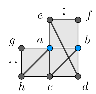
Figure 24.

1. Let us suppose that $a,b\in\mathcal{A}$. We discuss the following cases:

   1. If $c,d,e,f\notin\mathcal{A}$, then $g$ is a vertex in $\mathcal{A}$, otherwise we have a contradiction with (1)-(b) of Definition 5.9. Hence $[h,a]$ and $[c,b]$ are not in $\mathcal{C}_{\mathcal{A}}$ instead $[c,f]\in\mathcal{C}_{\mathcal{A}}$. Therefore, $\mathcal{C}_{\mathcal{A}}$ is a polyocollection which is not a collection of cells.

   2. We show firstly that $c$ cannot be in $\mathcal{A}$. If $c\in\mathcal{A}$, then $d\notin\mathcal{A}$, otherwise we have a contradiction with (1)-(b) of Definition 5.9, and, moreover, $e\in\mathcal{A}$ necessarily. Since $e\in\mathcal{A}$ and $f\notin\mathcal{A}$, then $e+(0,1)\in\mathcal{A}$. Continuing this argument for $e+(0,2)$, $e+(0,3)$ and so on, we can have two possibilities.

      • Suppose $[e,(m-1,n)]\subset\mathcal{A}$. We can assign the $2$-minor of $[h,a]$ to $c$, that one of $[c,b]$ to $a$, that one of $[c,f]$ to $b$ and that one of every cell in $\mathcal{P}_{[a,(m,n)]}$ to the lower left corner of the attached cell. Since $(m-1,n)$ is in $\mathcal{A}$, then it is clear that $|\mathcal{A}|+|F_{\mathcal{A}}|\geq|\mathcal{P}|+1$, which is a contradiction with (2) of Definition 5.9. For instance, look at the case dealing for $\mathcal{A}_{4}$ in Example 5.10.

      • Suppose there exists a vertex $v\in[e,(m-1,n-1)]$ such that $[e,v]\cup[v+(1,0),(m,n)]$ is in $\mathcal{A}$. Then we get the same previous contradiction by similar arguments.

      Hence $c$ cannot be in $\mathcal{A}$. Therefore, $g\in\mathcal{A}$ otherwise we have a contradiction with (1)-(b) of Definition 5.9. Hence $[h,a]$ and $[c,b]$ are not in $\mathcal{C}_{\mathcal{A}}$.

      1. Now, if $e,f\notin\mathcal{A}$, then $d\notin\mathcal{A}$, so $[c,f]\in\mathcal{C}_{\mathcal{A}}$. Therefore, $\mathcal{C}_{\mathcal{A}}$ is a polyocollection which is not a collection of cells.

      2. If either $e,f\in\mathcal{A}$ or $e\notin\mathcal{A}$ and $f\in\mathcal{A}$ (which implies $d\in\mathcal{A}$), then $[c,f]\notin\mathcal{C}_{\mathcal{A}}$, and if this holds even in the other three corners of $\mathcal{P}$, then $\mathcal{C}_{\mathcal{A}}$ is in particular a collection of cells.

2. When at least one of $a$ and $b$ is not in $\mathcal{A}$, then $\mathcal{P}$ is a collection of cells, since $[c,b]\notin\mathcal{C}_{\mathcal{A}}$ and $[c,f]\in\mathcal{C}_{\mathcal{A}}$ cannot be possible.

Now, we discuss some algebraic properties of $I_{\mathcal{C}}$, which will be useful in what follows. In particular, we show that $I_{\mathcal{C}_{\mathcal{A}}}$ is a prime ideal with $\mathrm{ht}(I_{\mathcal{C}_{\mathcal{A}}})=|F_{\mathcal{A}}|.$ We need to distinguish two cases.

• If $\mathcal{C}_{\mathcal{A}}$ is a collection of cells, in particular from the definition of $\mathcal{C}_{\mathcal{A}}$ we have that $\mathcal{C}_{\mathcal{A}}$ is either a simple polyomino or a disjoint union of simple polyominoes, so $I_{\mathcal{C}_{\mathcal{A}}}$ is a prime ideal from [23, Corollary 2.2] or [33, Corollary 2.3]. Moreover, from [25, Corollary 2.3] and [23, Corollary 2.2] it follows that $\mathrm{ht}(I_{\mathcal{C}_{\mathcal{A}}})=|\mathcal{C}_{\mathcal{A}}|$. Since there is a natural one-to-one correspondence between the cells of $\mathcal{C}_{\mathcal{A}}$ and the generators of $F_{\mathcal{A}}$, we have $|\mathcal{C}_{\mathcal{A}}|=|F_{\mathcal{A}}|$, so $\mathrm{ht}(I_{\mathcal{C}_{\mathcal{A}}})=|F_{\mathcal{A}}|.$

• If $\mathcal{C}$ is a polyocollection but not a collection of cells, that is in the cases $(1)-(a)$ and $(1)-(b)-(i)$, then $I_{\mathcal{C}_{\mathcal{A}}}$ can be identified with the inner $2$-minors ideal attached to the collection of cells $\mathcal{P}^{\prime}=\big{(}\mathcal{C}_{\mathcal{A}}\setminus\{[c,f]\}\big{)}\cup\{[a,f]\}$. We are replacing just an interval with a cell in $\mathcal{C}_{\mathcal{A}}$, so $\mathcal{P}^{\prime}$ is a simple polyomino or a disjoint union of simple polyominoes, so $I_{\mathcal{C}_{\mathcal{A}}}$ is a prime ideal $\mathrm{ht}(I_{\mathcal{C}_{\mathcal{A}}})=|F_{\mathcal{A}}|$ by the same arguments done before.

From Discussion 5.11 we get the following result.

Lemma 5.12.

Let $\mathcal{P}$ be a circle closed path polyomino, $J(\mathcal{P})$ be the ideal as in Definition 5.2 and $\mathcal{A}$ be an admissible set for $J(\mathcal{P})$. Let $F_{\mathcal{A}}$ be the set of the generators $f$ of $J(\mathcal{P})$ such that $V(f)\cap\mathcal{A}=\emptyset$. Then

$$\mathcal{C}_{\mathcal{A}}=\{I\ \text{is an interval of}\ \mathbb{Z}^{2}:V(I)=V(f)\ \text{for some}\ f\in F_{\mathcal{A}}\}$$

is a polyocollection $\mathcal{C}_{\mathcal{A}}$ such that $I_{\mathcal{C}_{\mathcal{A}}}$ is a prime ideal and $\mathrm{ht}(I_{\mathcal{C}_{\mathcal{A}}})=|F_{\mathcal{A}}|.$

Now, if $\mathcal{A}\subset V(\mathcal{P})$ is an admissible set for $J(\mathcal{P})$, then we set $X(\mathcal{A})=\{x_{a}:a\in\mathcal{A}\}$.

Lemma 5.13.

Let $\mathcal{P}$ be a circle closed path polyomino and $J(\mathcal{P})$ be the ideal as in Definition 5.2. Let $\mathcal{A}$ be an admissible set for $J(\mathcal{P})$ and $\mathcal{C}_{\mathcal{A}}$ be the polyocollection defined in Lemma 5.12. Consider the ideal $\mathfrak{p}_{\mathcal{A}}=I_{\mathcal{C}_{\mathcal{A}}}+(X(\mathcal{A}))$ in $S_{\mathcal{P}}$. Then $\mathfrak{p}_{\mathcal{A}}$ is a minimal prime ideal of $J(\mathcal{P})$.

Proof.

We start by showing that $J(\mathcal{P})$ is contained in $\mathfrak{p}_{\mathcal{A}}$. Let $f$ be a generator of $J(\mathcal{P}).$ If $f$ is in $F_{\mathcal{A}}$, then $f$ is a generator of $I_{\mathcal{C}_{\mathcal{A}}}$. By contradiction, if we assume that $f\notin F_{\mathcal{A}}$, then $V(f)\cap\mathcal{A}$ contains at least an edge of $f$, which means that a diagonal corner and an anti-diagonal one of the interval given by $V(f)$ are in $\mathcal{A}$, so $f$ belongs to $(X(\mathcal{A}))$. Hence, $J(\mathcal{P})$ is contained in $\mathfrak{p}_{\mathcal{A}}$.
Let us consider the ideal $(X(\mathcal{A}))$. It is generated by $|\mathcal{A}|$ variables, so it is a prime ideal with $\mathrm{ht}(X(\mathcal{A}))=|\mathcal{A}|.$ By Lemma 5.12, we know that $\mathcal{C}_{\mathcal{A}}$ is a polyocollection such that $I_{\mathcal{C}_{\mathcal{A}}}$ is a prime ideal and $\mathrm{ht}(I_{\mathcal{C}_{\mathcal{A}}})=|F_{\mathcal{A}}|.$ Now, we observe that for any generator $f$ of $I_{\mathcal{C}_{\mathcal{A}}}$ and for any $a\in\mathcal{A}$, we have $\mathrm{supp}(f)\cap\mathrm{supp}(x_{a})=\emptyset$. Hence $\mathfrak{p}_{\mathcal{A}}$ is a prime ideal with $\mathrm{ht}(\mathfrak{p}_{\mathcal{A}})=|F_{\mathcal{A}}|+|\mathcal{A}|,$ which is $|\mathcal{P}|$ from Definition 5.9, that is the height of $J(\mathcal{P})$, by Lemma 5.8. Then, $\mathfrak{p}_{\mathcal{A}}$ is a minimal prime of $J(\mathcal{P}).$ ∎

Lemma 5.14.

Let $\mathcal{P}$ be a circle closed path polyomino and $J(\mathcal{P})$ be the ideal as in Definition 5.2. Let $\mathfrak{p}$ be a minimal prime of $J(\mathcal{P})$. Then there exists an admissible set $\mathcal{A}$ for $J(\mathcal{P})$ such that $\mathfrak{p}=\mathfrak{p}_{\mathcal{A}}$.

Proof.

Let $\mathcal{A}=\{a\in V(\mathcal{P}):x_{a}\in\mathfrak{p}\}$. We want to prove that $\mathcal{A}$ is an admissible set of $J(\mathcal{P})$ such that $\mathfrak{p}=\mathfrak{p}_{\mathcal{A}}$. If $\mathcal{A}=\emptyset$, then $\mathcal{A}$ is an admissible set for $J(\mathcal{P})$. Moreover, in order to prove that $\mathfrak{p}=\mathfrak{p}_{\emptyset}:=I_{\mathcal{P}}$, we show firstly that $I_{\mathcal{P}}\subset\mathfrak{p}$. By being the structure of $\mathcal{P}$ and the definition of $J(\mathcal{P})$ and $I_{\mathcal{P}}$, it is enough to prove that $x_{c}x_{f}-x_{e}x_{b}$ and $x_{a}x_{f}-x_{d}x_{e}$, as in Figure 25 (A) and (B) respectively, belong to $\mathfrak{p}$.

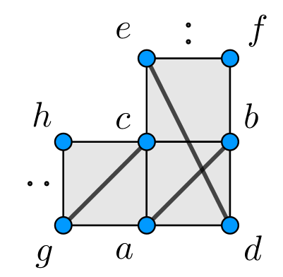
(a)

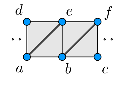
(b)

Figure 25.

Observe that $x_{a}(x_{c}x_{f}-x_{e}x_{b})\in\mathfrak{p}$ because $x_{a}(x_{c}x_{f}-x_{e}x_{b})=x_{c}(x_{a}x_{f}-x_{e}x_{b})-x_{e}(x_{a}x_{d}-x_{c}x_{b})$ and $x_{a}x_{f}-x_{e}x_{b},x_{a}x_{d}-x_{c}x_{b}\in J(\mathcal{P})\subset\mathfrak{p}$. So, $x_{c}x_{f}-x_{e}x_{b}\in\mathfrak{p}$ because $\mathfrak{p}$ is prime and $x_{a}\notin\mathfrak{p}$. Similarly, $x_{e}(x_{a}x_{f}-x_{d}x_{c})=x_{f}(x_{a}x_{e}-x_{d}x_{b})+x_{d}(x_{b}x_{f}-x_{e}x_{c})\in\mathfrak{p}$, so $x_{a}x_{f}-x_{d}x_{c}\in\mathfrak{p}.$ Therefore $I_{\mathcal{P}}\subset\mathfrak{p}$. Observe that $I_{\mathcal{P}}$ is a prime ideal by [3, Corollary 4.3] and $J(\mathcal{P})\subset I_{\mathcal{P}}\subset\mathfrak{p}$ so $I_{\mathcal{P}}=\mathfrak{p}$ from the minimality of $\mathfrak{p}$.
Now, assume that $\mathcal{A}\neq\emptyset$. Let us show that $\mathcal{A}$ is an admissible set for $J(\mathcal{P}).$ Suppose by contradiction that $\mathcal{A}$ is not an admissible set for $J(\mathcal{P})$, so at least one of the conditions in Definition 5.9 does not hold. We need to analyze some cases.

• Suppose that there exists a generator $f=x_{p}x_{q}-x_{r}x_{s}$ of $J(\mathcal{P})$, where $p,q$ and $r,s$ are diagonal and anti-diagonal corners of $f$ respectively, such that $V(f)\cap\mathcal{A}$ does not contains an edge of $f$ or $V(f)\cap\mathcal{A}=V(f).$

  1. Assume that $V(f)\cap\mathcal{A}$ does not contains an edge of $f$, so either $|V(f)\cap\mathcal{A}|=1$ or $V(f)\cap\mathcal{A}$ contains $p,q$ (or $r,s$). If $|V(f)\cap\mathcal{A}|=1$, then we may assume that $V(f)\cap\mathcal{A}=\{p\}$, so $x_{r}x_{s}\in\mathfrak{p}$ since $f,x_{p}\in\mathfrak{p}$. Hence $x_{r}\in\mathfrak{p}$ or $x_{s}\in\mathfrak{p}$ because of the primality of $\mathfrak{p}$, so $V(f)\cap\mathcal{A}$ contains an edge of $f$, which is a contradiction. The same argument holds if $V(f)\cap\mathcal{A}$ contains $p,q$ (or $r,s$).

  2. Assume that $V(f)\cap\mathcal{A}=V(f).$ With reference to Figure 25 (A), set $p=a$ and $q=b$, so $r=c$ and $s=d$. Let $F_{\mathcal{A}}$ be the set of the generators $f$ of $J(\mathcal{P})$ such that $V(f)\cap\mathcal{A}=\emptyset$ and $\mathcal{C}_{\mathcal{A}}$ be the polyocollection defined by the intervals $I$ of $\mathbb{Z}^{2}$ such that $V(I)=V(f)$, for some $f\in F_{\mathcal{A}}$. Denote $X_{b}=\{x_{v}:v\in\mathcal{A}\setminus\{b\}\}$. Consider $\mathfrak{p}^{\prime}:=I_{\mathcal{C}_{\mathcal{A}}}+(X_{b})$. It is easy to see, as in Lemma 5.13, that $J(\mathcal{P})\subset\mathfrak{p}^{\prime}$ and $\mathfrak{p}^{\prime}$ is prime. Moreover, as done before, it can be shown that $I_{\mathcal{C}_{\mathcal{A}}}\subset\mathfrak{p}$, so $\mathfrak{p}^{\prime}\subset\mathfrak{p}$. From the minimality of $\mathfrak{p}$, we have $\mathfrak{p}^{\prime}=\mathfrak{p}$, but this is a contradiction since $x_{b}\in\mathfrak{p}$ but $x_{b}\notin\mathfrak{p}^{\prime}$. Similar arguments can be made for the case $p=a$ and $q=f$, referring to Figure 25 (A). Now, we refer to Figure 25 (B) and assume that $p=a$ and $q=e$, so $r=d$ and $s=b$. In such a case, consider $F_{\mathcal{A}\setminus\{e,b\}}$ as the set of the generators $f$ of $J(\mathcal{P})$ such that $V(f)\cap(\mathcal{A}\setminus\{e,b\})=\emptyset$, $\mathcal{C}_{\mathcal{A}}$ as the polyocollection defined by the intervals $I$ of $\mathbb{Z}^{2}$ such that $V(I)=V(f)$, for some $f\in F_{\mathcal{A}\setminus\{e,b\}}$, $X_{e,b}:=\{x_{v}:v\in\mathcal{A}\setminus\{e,b\}\}$ and $\mathfrak{p}^{\prime}:=I_{\mathcal{C}_{\mathcal{A}}}+(X_{e,b})$. Arguing as done before we get $\mathfrak{p}=\mathfrak{p}^{\prime}$, so a contradiction arises also in this case.

• Here we discuss the case when $|F_{\mathcal{A}}|+|\mathcal{A}|\neq|\mathcal{P}|$, where $F_{\mathcal{A}}$ is the set of the generators $f$ of $J(\mathcal{P})$ such that $V(f)\cap\mathcal{A}=\emptyset$. First of all, we observe that $b$ in Figure 25 (A) is the diagonal corner of the only binomial $x_{a}x_{b}-x_{c}x_{d}$ and $d$ is the anti-diagonal corner of the binomials $x_{a}x_{b}-x_{c}x_{d}$ and $x_{a}x_{f}-x_{e}x_{d}$; the other vertices in Figures 25 (A), except $b$ and $d$, and (B) at the same time diagonal and anti-diagonal corner of two different generators of $J(\mathcal{P})$, for instance, $a$ is diagonal corner of $x_{a}x_{b}-x_{c}x_{d}$ and anti-diagonal of $x_{g}x_{c}-x_{h}x_{a}$.
  Now, suppose that $|F_{\mathcal{A}}|+|\mathcal{A}|\neq|\mathcal{P}|.$ Denote by $\mathcal{G}(J(\mathcal{P}))$ the set of generators of $J(\mathcal{P})$ and recall that $|J(\mathcal{P})|=|\mathcal{P}|$. This means that we are assuming that $|\mathcal{A}|\neq|\mathcal{G}(J(\mathcal{P}))\setminus F_{\mathcal{A}}|$. Consider $|\mathcal{A}|<|\mathcal{G}(J(\mathcal{P}))\setminus F_{\mathcal{A}}|$. Hence, $|\mathcal{A}|<|\mathcal{G}(J(\mathcal{P}))\setminus F_{\mathcal{A}}|$ implies that there exist two binomials $F$ and $G$ in $\mathcal{G}(J(\mathcal{P}))\setminus F_{\mathcal{A}}$ such that $V(F)\cap\mathcal{A}$ and $V(G)\cap\mathcal{A}$ consist of the same vertex, which we may assume that is a diagonal corner, and the anti-diagonal corners of $F$ and $G$ are not in $\mathcal{A}$. With reference to Figure 25 (B), for instance, it means that if $F=x_{a}x_{e}-x_{d}x_{b}$, $G=x_{b}x_{f}-x_{e}x_{c}$ and $b\in\mathcal{A}$, then $a,e,c\notin\mathcal{A}$. But this leads a contradiction since $F,x_{b}\in\mathfrak{p}$ so $x_{a}\in\mathfrak{p}$ or $x_{e}\in\mathfrak{p}$ for the primality of $\mathfrak{p}$. All the other possible situations of $F$ and $G$ coming from Figure 25 (A) give us a similar contradiction.
  Now, assume that $|\mathcal{A}|>|\mathcal{G}(J(\mathcal{P}))\setminus F_{\mathcal{A}}|$. Recall also that $|\mathcal{P}|=\frac{|V(\mathcal{P})|}{2}$. Since $|\mathcal{A}|>|\mathcal{G}(J(\mathcal{P}))\setminus F_{\mathcal{A}}|$ then every segment in Figures 25 (A) and (B) has a point in $\mathcal{A}$, and there exists a segment having two vertices in $\mathcal{A}$. This leads to a contradiction. In fact, with reference to Figure 25 (A), we suppose that $b,c,d,e\in\mathcal{A}$. Observe that $a\notin\mathcal{A}$, otherwise we have $V(x_{a}x_{b}-x_{c}x_{d})\cap\mathcal{A}=V(x_{a}x_{b}-x_{c}x_{d})$ and we have a contradiction as in Case 1)-(2). If $f\notin\mathcal{A}$, then the contradiction arises as $x_{a}\in\mathfrak{p}$ or $x_{f}\in\mathfrak{p}.$ So, $f\in\mathcal{A}$. But, in such a case, consider $F_{\mathcal{A}\setminus\{d\}}$ as the set of the generators $f$ of $J(\mathcal{P})$ such that $V(f)\cap(\mathcal{A}\setminus\{d\})=\emptyset$, $\mathcal{C}_{\mathcal{A}}$ as the polyocollection defined by the intervals $I$ of $\mathbb{Z}^{2}$ such that $V(I)=V(f)$, for some $f\in F_{\mathcal{A}\setminus\{d\}}$, $X_{d}:=\{x_{v}:v\in\mathcal{A}\setminus\{d\}\}$ and $\mathfrak{p}^{\prime}:=I_{\mathcal{C}_{\mathcal{A}}}+(X_{d})$. Arguing as in Case 1)-(2) we get $\mathfrak{p}=\mathfrak{p}^{\prime}$, which leads to a contradiction. All other cases, coming by taking other different points, give us a contradiction as got before. Moreover, referring to Figure 25 (B), we may suppose that $b,d,e,f\in\mathcal{A}$. This case leads to a contradiction arguing as done before, considering $F_{\mathcal{A}\setminus\{b\}}$ as the set of the generators $f$ of $J(\mathcal{P})$ such that $V(f)\cap(\mathcal{A}\setminus\{b\})=\emptyset$, $\mathcal{C}_{\mathcal{A}}$ as the polyocollection defined by the intervals $I$ of $\mathbb{Z}^{2}$ such that $V(I)=V(f)$, for some $f\in F_{\mathcal{A}\setminus\{b\}}$, $X_{b}:=\{x_{v}:v\in\mathcal{A}\setminus\{b\}\}$ and $\mathfrak{p}^{\prime}:=I_{\mathcal{C}_{\mathcal{A}}}+(X_{b})$.
  We have a contradiction when $|F_{\mathcal{A}}|+|\mathcal{A}|\neq|\mathcal{P}|$, so we get the claim: $|F_{\mathcal{A}}|+|\mathcal{A}|=|\mathcal{P}|$.

Therefore, we have proved that $\mathcal{A}$ is an admissible set of $J(\mathcal{P}).$ Now, we need to show only that $\mathfrak{p}=\mathfrak{p}_{\mathcal{A}}$. Consider the prime ideal $\mathfrak{p}_{\mathcal{A}}=I_{\mathcal{C}_{\mathcal{A}}}+(X(\mathcal{A}))$. As done for the first part of the proof, where we proved that $\mathfrak{p}=I_{\mathcal{P}}$, we have that $\mathfrak{p}_{\mathcal{A}}\subset\mathfrak{p}$. Then, by the minimality of $\mathfrak{p}$, we have $\mathfrak{p}=\mathfrak{p}_{\mathcal{A}}$. ∎

Theorem 5.15.

Let $\mathcal{P}$ be a circle closed path polyomino and $J(\mathcal{P})$ be the ideal as in Definition 5.2. An ideal $\mathfrak{p}$ is a minimal prime of $J(\mathcal{P})$ if and only if $\mathfrak{p}=I_{\mathcal{C}_{\mathcal{A}}}+(X(\mathcal{A}))$, where $\mathcal{A}$ is an admissible set for $J(\mathcal{P})$ and $\mathcal{C}_{\mathcal{A}}$ is the polyocollection defined in Lemma 5.12. In particular, $J(\mathcal{P})$ is an unmixed ideal.

Proof.

It follows from Lemma 5.13 and 5.14. Moreover, all the minimal primes of $J(\mathcal{P})$ have the same height, hence $J(\mathcal{P})$ is unmixed. ∎

Example 5.16.

Consider the circle closed path $\mathcal{P}$ as in Figure 23. Using Macaulay2 and the package Binomials (see [40]), we compute all the minimal primes of $J(\mathcal{P})$, which are $1448$. Here, we figure out just some of them.

1. $\mathfrak{p}_{1}=I_{\mathcal{C}_{1}}+M_{1}$, where $M_{1}=(x_{(6,5)},\,x_{(6,4)},\,x_{(6,3)},\,x_{(6,2)},\,x_{(6,1)})$ and $I_{\mathcal{C}_{1}}$ is the ideal attached to the collection of white cells in Figure 26 (A);

2. $\mathfrak{p}_{2}=I_{\mathcal{C}_{2}}+M_{2}$, where $M_{2}=(x_{(1,5)},\,x_{(2,5)},\,x_{(5,5)},\,x_{(2,4)},\,x_{(5,4)},x_{(5,3)},\,x_{(5,2)},\,x_{(5,1)})$ and $I_{\mathcal{C}_{2}}$ is the ideal attached to the polyocollection

   $$\mathcal{C}_{2}=\big{\{}[(1,1),(2,2)],[(1,2),(2,3)],[(2,1),(3,2)],[(3,1),(4,2)],[(3,4),(4,5)],[(4,4),(6,5)]\big{\}}.$$

   Look at Figure 26 (B);

3. $\mathfrak{p}_{3}=(x_{(1,5)},\,x_{(1,4)},\,x_{(1,3)},\,x_{(1,2)},\,x_{(1,1)},x_{(2,4)},\,x_{(3,4)},\,x_{(4,4)},\,x_{(4,2)},\,x_{(4,1)},\,x_{(5,4)},\,x_{(5,1)},\,x_{(6,4)},\,x_{(6,1)})$. Look at Figure 26 (C).

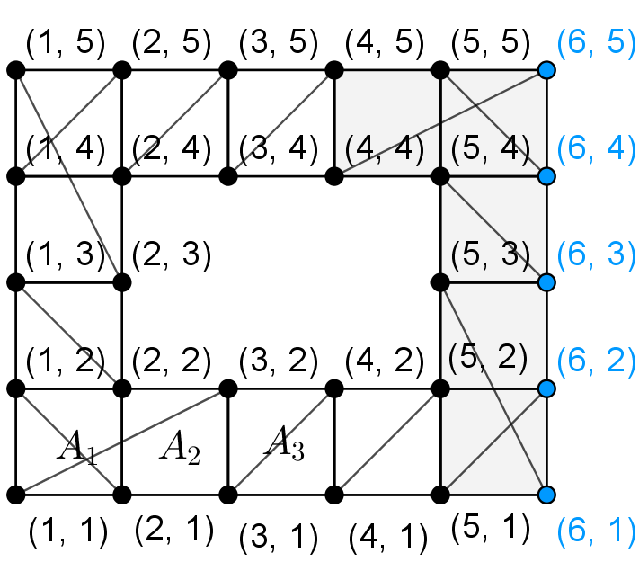
(a)

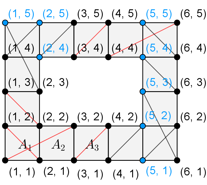
(b)

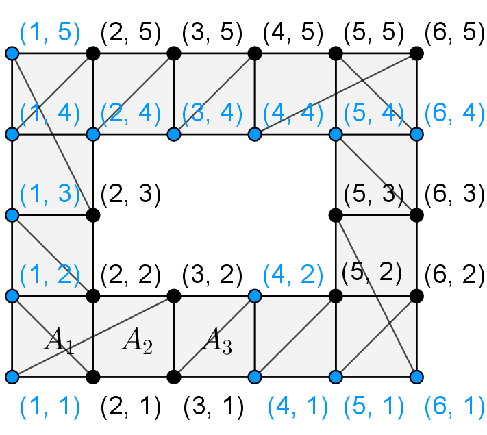
(c)

Figure 26.

Now, we are ready to prove Theorem 5.4.

Proof of Theorem 5.4.

Let $\mathcal{P}$ be a circle closed path polyomino and $J(\mathcal{P})$ and $K(\mathcal{P})$ be the ideals as in Definition 5.2. We want to show that $J(\mathcal{P}):I_{\mathcal{P}}=J(\mathcal{P})+K(\mathcal{P})$. We denote

$$T(\mathcal{P}):=\bigcap_{\mathcal{A}\text{ admissible set}\atop\text{ of }J(\mathcal{P})\text{ with }\mathcal{A}\neq\emptyset}\Big{(}I_{\mathcal{C}_{\mathcal{A}}}+(X(\mathcal{A}))\Big{)}.$$

By Proposition 5.7, Lemma 5.8 and Theorem 5.15 we have $J(\mathcal{P}):I_{\mathcal{P}}=T(\mathcal{P})$. We prove that $J(\mathcal{P})+K(\mathcal{P})=T(\mathcal{P})$.
$\subseteq)$ Let $f$ be a generator of $J(\mathcal{P})+K(\mathcal{P})$. Firstly, consider that $f$ is a generator of $J(\mathcal{P})$, as $x_{a}x_{b}-x_{c}x_{d}$, and we show that $f\in I_{\mathcal{C}_{\mathcal{A}}}+(X(\mathcal{A}))$ for all admissible set $\mathcal{A}\neq\emptyset$ of $J(\mathcal{P})$. Let $\mathcal{A}$ be an admissible set of $J(\mathcal{P})$, different from the empty set. If $V(f)\cap\mathcal{A}=\emptyset$, then $f$ is a generator of $I_{\mathcal{C}_{\mathcal{A}}}$. Assume that $V(f)\cap\mathcal{A}=\emptyset$ contains an edge of $f$, so we may consider that $\{a,c\}\in V(f)\cap\mathcal{A}$. This implies that $f\in(X(\mathcal{A}))$, so $f\in I_{\mathcal{C}_{\mathcal{A}}}+(X(\mathcal{A}))$. Now, suppose that $f$ is a monomial generator of $K(\mathcal{P})$. Using notations from Definition 5.2, we have that

$$f=x_{v_{1}}x_{v_{2}}\dots x_{v_{t}}x_{(2,2)}x_{(1,n)}x_{(m,1)}x_{(m-1,n-1)}$$

for some $(v_{1},v_{2},\dots,v_{t})\in\mathcal{V}$. It is enough to show that for any admissible set $\mathcal{A}\neq\emptyset$, there exists a vertex $w\in\{v_{i}:i\in[t]\}\cup\{(2,2),(1,n),(m,1),(m-1,n-1)\}$ such that $w\in\mathcal{A}$, so that $f\in(X(\mathcal{A}))$. Let us suppose by contradiction that there exists an admissible set $\mathcal{A}\neq\emptyset$ such that every vertex in $\{v_{i}:i\in[t]\}\cup\{(2,2),(1,n),(m,1),(m-1,n-1)\}$ does not belong to $\mathcal{A}$. Without loss of generality, we may consider only the part of $\mathcal{P}$ as in Figure 27, where $a=(m-1,2)$ and $b=(m,2)$, since $\mathcal{P}$ consists only suitable rotations of this type of configuration. With reference to Figure 27 we have that $d,a^{\prime}\notin\mathcal{A}$. Consider $a_{1}$ and $b_{1}$. Using our assumption, we have $a_{1}\notin\mathcal{A}$ or $b_{1}\notin\mathcal{A}$. If $a_{1}\notin\mathcal{A}$ and $b_{1}\in\mathcal{A}$, then we obtain a contradiction, because $a_{1},d\notin\mathcal{A}$, hence $\mathcal{A}$ cannot be an admissible set for $J(\mathcal{P})$, because the condition (1) of Definition 5.9 is not satisfied. If $a_{1}\in\mathcal{A}$ and $b_{1}\notin\mathcal{A}$, then $a_{2}\in\mathcal{A}$, because $\mathcal{A}$ is an admissible set for $J(\mathcal{P})$, so $b_{2}$ cannot be in $\mathcal{A}$ from our assumption. Continuing this arguments until $a_{n-4}$, we get that $a_{n-4}\in\mathcal{A}$ and $b_{n-4}\notin\mathcal{A}$. Since $\mathcal{A}$ is an admissible set for $J(\mathcal{P})$ and $b_{n-4}\notin\mathcal{A}$, then $a^{\prime}\in\mathcal{A}$ but this is a contradiction since $a^{\prime}\notin\mathcal{A}$. Hence $a_{1},b_{1}$ cannot be in $\mathcal{A}$. These arguments can be repeated for any $a_{i}$ and $b_{i}$, where $i=2,\dots,n-4$, getting that $a_{i},b_{i}\notin\mathcal{A}$ for all $i\in[n-4]$. Therefore, the only vertices in $\mathcal{A}$ can be $a,c,b,c^{\prime},b^{\prime},d^{\prime}$ and the analogous six vertices in the other two changes of direction. But it is impossible to make an admissible set with just these vertices, so $\mathcal{A}$ cannot be an admissible set for $J(\mathcal{P})$, which is a contradiction. Hence, $f\in(X(\mathcal{A}))$ and, in conclusion, $J(\mathcal{P})+K(\mathcal{P})\subseteq T(\mathcal{P})$.

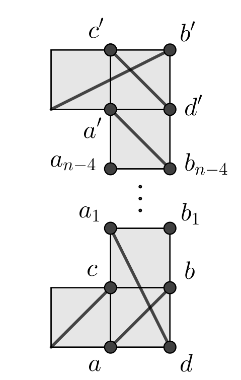
Figure 27.

$\supseteq)$ Now, let $f\in T(\mathcal{P})$, so $f\in I_{\mathcal{C}_{\mathcal{A}}}+(X(\mathcal{A}))$ for all admissible set $\mathcal{A}\neq\emptyset$. If $f\in J(\mathcal{P})$ then we have finished. Assume that $f\notin J(\mathcal{P})$ and we prove that $f\in K(\mathcal{P})$. Suppose that $f\notin K(\mathcal{P})$. Then it follows that there exists $m\in\mathrm{supp}(f)$ such that $m\notin K(\mathcal{P})$. We need to examine two cases.

1. With reference to the notations in Definition 5.9, suppose that there is a component $\mathcal{A}_{1}=\{a,b\}$ of $\mathcal{V}$ such that $x_{a}$ and $x_{b}$ do not divide $m$. It is not restrictive to assume that $\mathcal{A}_{1}=\{a_{1},b_{1}\}$, referring to Figure 27, because the arguments are the same if $\mathcal{A}_{1}$ is in $\{R_{j}:j=4,\dots,n-2\}$, $\{L_{j}:j=3,\dots,n-2\}$, $\{U_{k}:k=3,\dots,m-2\}$ or $\{D_{k}:j=3,\dots,m-2\}$. Observe that $\mathcal{A}_{1}$ is an admissible set for $J(\mathcal{P})$ and $m\notin(X(\mathcal{A}_{1}))$, so $f$ does not belong to $(X(\mathcal{A}_{1}))$. Since $f\in T(\mathcal{P})$, then $f\in I_{\mathcal{C}_{\mathcal{A}_{1}}}$, where $\mathcal{C}_{\mathcal{A}_{1}}$ is the polyomino obtaining by $\mathcal{P}$ removing the cells having $\{a,b\}$ as common edge. Hence $f\in I_{\mathcal{P}}$.

2. The other case so that $m\notin K(\mathcal{P})$ is $x_{d}$ does not divide $m$ (or $a^{\prime}$ does not divide $m$). Taking $\mathcal{A}=\{a,c,d\}$ as an admissible set and using some arguments as done before, we get $f\in I_{\mathcal{P}}$.

Hence, we obtain that $f\in I_{\mathcal{P}}$ in both cases. Since $f\in T(\mathcal{P})$, then it follows that $f\in T(\mathcal{P})\cap I_{\mathcal{P}}$. Recall that $J(\mathcal{P})$ is a radical ideal from Lemma 5.8 and, moreover, $I_{\mathcal{P}}$ is the minimal prime of $J(\mathcal{P})$ coming from $\emptyset$ as an admissible set. By being $J(\mathcal{P})$ radical, we have that $J(\mathcal{P})$ is the intersection of all minimal prime ideals of $J(\mathcal{P})$, so $T(\mathcal{P})\cap I_{\mathcal{P}}=J(\mathcal{P})$. Hence, we get that $f\in J(\mathcal{P})$, which is a contradiction. Therefore, $T(\mathcal{P})\subseteq J(\mathcal{P})+K(\mathcal{P})$.
We have that $J(\mathcal{P}):I_{\mathcal{P}}=J(\mathcal{P})+K(\mathcal{P})$, and by Proposition 5.6, we obtain the desired conclusion, namely

$$\omega_{K[\mathcal{P}]}\cong\big{(}J(\mathcal{P})+K(\mathcal{P})\big{)}/J(\mathcal{P}).$$

∎

Example 5.17.

Let $\mathcal{P}$ be closed path polyomino in Figure 28. By using Macaulay2, we observe that $J(\mathcal{P}):I_{\mathcal{P}}=J(\mathcal{P})+K(\mathcal{P})$, where $K(\mathcal{P})$ is still a squarefree monomial ideal but it is not equigenerated, which means that it is not generated in a single degree. For instance, two generators of $K(\mathcal{P})$ in different degrees are $x_{(1,2)}x_{(1,3)}x_{(1,4)}x_{(2,6)}x_{(3,1)}x_{(3,6)}x_{(4,1)}x_{(4,6)}x_{(5,1)}x_{(6,3)}x_{(6,4)}x_{(6,5)}$ and $x_{(1,4)}x_{(2,2)}x_{(2,3)}x_{(3,2)}x_{(3,6)}x_{(4,3)}x_{(4,5)}x_{(5,1)}x_{(6,4)}$.

Figure 28.

Question. Is it possible to give a combinatorial interpretation of the canonical module of a closed path, whose coordinate ring is Cohen-Macaulay, or more in general for other classes of polyominoes?

The description of the canonical module of $K[\mathcal{P}]$ given in Theorem 5.4 allows us to compute the Cohen-Macaulay type of $K[\mathcal{P}]$, i.e. the number of generators of the canonical module, where $\mathcal{P}$ is a circle closed path polyomino. As a consequence, we show that $K[\mathcal{P}]$ is a level ring, i.e. the generators of $\omega_{K[\mathcal{P}]}$ are of the same degree.

Corollary 5.18.

Let $\mathcal{P}$ be a circle closed path polyomino. Then:

$$\mathrm{type}(K[\mathcal{P}])=\left\{\begin{array}[]{ll}1,&m=n=4;\\ (m-3)^{2}(n-3)^{2},&m,n>4;\\ (n-3)^{2},&m=4,n>4;\\ (m-3)^{2},&m>4,n=4.\\ \end{array}\right.$$

Moreover, $K[\mathcal{P}]$ is a level ring.

Proof.

If $m=n=4$, then $K[\mathcal{P}]$ is Gorenstein, hence $\mathrm{type}(K[\mathcal{P}])=1$. Assume that $m,n>4$. From [41, Corollary 5.3.6], the Cohen-Macaulay type of $K[\mathcal{P}]$ is equal to the minimum number of the generators of the canonical module of $K[\mathcal{P}]$. The set $\mathcal{G}=\{{\mathbf{x_{v}}}+J(\mathcal{P}):\mathbf{v}\in\mathcal{V}\}$ is a set of generators of $(J(\mathcal{P})+K(\mathcal{P}))/J(\mathcal{P})$. We need to show that $\mathcal{G}$ minimally generates $(J(\mathcal{P})+K(\mathcal{P}))/J(\mathcal{P})$. Suppose by contradiction that $\mathcal{G}$ is not a set of minimum number of generators of $(J(\mathcal{P})+K(\mathcal{P}))/J(\mathcal{P})$, so there exists $\mathbf{w}\in\mathcal{V}$ such that $\mathbf{x}_{\mathbf{w}}$ belongs to the ideal $J(\mathcal{P})+(\mathbf{x}_{\mathbf{v}}:\mathbf{v}\in\mathcal{V}\setminus\{\mathbf{w}\})$. Set $J^{\prime}=J(\mathcal{P})+(\mathbf{x}_{\mathbf{v}}:\mathbf{v}\in\mathcal{V}\setminus\{\mathbf{w}\})$ and $\mathcal{G}(J^{\prime})=\{f:f\text{ generator of }J(\mathcal{P})\}\cup\{\mathbf{x}_{\mathbf{v}}:\mathbf{v}\in\mathcal{V}\setminus\{\mathbf{w}\}\}$. Let $<$ be the lexicographic order on $S_{\mathcal{P}}$ defined in Proposition 4.7. Denote by $S(f,g)$ the $S$-polynomial of two polynomial $f$ and $g$ of $S_{\mathcal{P}}$. We note the following properties.

1. For any two generators $f,g$ of $J(\mathcal{P})$, $S(f,g)$ reduces to $0$ since $\mathrm{gcd}(\mathrm{in}_{<}(f),\mathrm{in}_{<}(g))=1$.

2. Trivially $S(u,u^{\prime})=0$ for all monomial $u$ and $u^{\prime}$ in $S_{\mathcal{P}}$.

3. Consider a monomial $m$ in $S_{\mathcal{P}}$ and suppose that there exists a generator $f$ of $J(\mathcal{P})$ such that $\mathrm{in}_{<}(f)$ divides $m$. Then $m=\mathrm{in}_{<}(f)u$, for a suitable monomial in $S_{\mathcal{P}}$, and we may write $f$ as $\pm\mathrm{in}_{<}(f)\mp f^{\prime}$. Hence by dividing $m$ with respect to $f$, we have $m=(\pm u)(\pm\mathrm{in}_{<}(f)\mp f^{\prime})+uf^{\prime}$. The latter means that $m$ reduces to $uf^{\prime}$ with respect to $f$, where $f^{\prime}$ is a monomial related to either diagonal or anti-diagonal corners of $V(f)$.

4. Consider a monomial $m$ in $S_{\mathcal{P}}$ and assume that there exists a generator $f$ of $J(\mathcal{P})$ such that, if $\mathrm{in}_{<}(f)=x_{a}x_{b}$ ($a,b\in V(\mathcal{P})$), then $m=ux_{a}$ for a suitable monomial $u$ in $S_{\mathcal{P}}$ and $x_{b}$ does not divide $u$. Then $S(m,f)=\pm uf^{\prime}$, where $\deg(uf^{\prime})>\deg(m)$, and it cannot be reduced to $0$ modulo $\mathcal{G}(J^{\prime})$ from the arguments used in $(3)$.

5. If $m$ is a monomial in $S_{\mathcal{P}}$ and suppose that there exists a generator $f$ of $J(\mathcal{P})$ such that $\mathrm{in}_{<}(f)$ divides $m$, then $S(m,f)=\pm uf^{\prime}$, where $\deg(uf^{\prime})=\deg(m)$, and it cannot be reduced to $0$ modulo $\mathcal{G}(J^{\prime})$ as well.

Denote by $\mathfrak{G}$ the Gröbner basis of $J^{\prime}$ with respect to $<$. From the properties described above, we can easily deduce that $\mathbf{x}_{\mathbf{w}}$ cannot be reduced to $0$ modulo $\mathfrak{G}$, which is a contradiction, since $\mathbf{x}_{\mathbf{v}}\in J^{\prime}$. Therefore, $\mathcal{G}$ is a minimal set of generators of $(J(\mathcal{P})+K(\mathcal{P}))/J(\mathcal{P})$. By Remark 5.3, it follows that $\mathrm{type}(K[\mathcal{P}])=(m-3)^{2}(n-3)^{2}$. Finally, since the monomials in $\mathcal{G}$ have the same degree, $K[\mathcal{P}]$ is a level ring. Similar arguments can be used in the cases $m=4,n>4$ and $m>4,n=4$. ∎

Question. Is it possible to give an estimate, or an upper bound or a lower bound at least, for the Cohen-Macaulay type in terms of the combinatorial properties of a polyomino?

References

- [1]
- [2] W. Bruns, J. Herzog, Cohen–Macaulay rings, Cambridge University Press, London, Cambridge, New York, 1993.
- [3] C. Cisto, F. Navarra, Primality of closed path polyominoes, Journal of Algebra and its Applications, Vol. 22, No. 02, 2350055, 2023.
- [4] C. Cisto, F. Navarra, R. Jahangir, PolyominoIdeals - a package to deal with polyomino ideals, Macaulay2, available at https://macaulay2.com/doc/Macaulay2/share/doc/Macaulay2/PolyominoIdeals/html/index.html.
- [5] C. Cisto, F. Navarra, R. Jahangir, On algebraic properties of some non-prime ideals of collections of cells, preprint arXiv:2401.09152, 2024.
- [6] C. Cisto, F. Navarra, R. Utano, Primality of weakly connected collections of cells and weakly closed path polyominoes, Illinois Math. Journal, 1-19, 2022.
- [7] C. Cisto, F. Navarra, R. Utano, On Gröbner bases and Cohen-Macaulay property of closed path polyominoes, The Electronic Journal of Combinatorics, 29, 3, 2022.
- [8] C. Cisto, F. Navarra, R. Utano, Hilbert-Poincaré series and Gorenstein property for some non-simple polyominoes, Bulletin of the Iranian Mathematical Society, 49, 22 (2023).
- [9] C. Cisto, F. Navarra, D. Veer, Polyocollection ideals and primary decomposition of polyomino ideals, J. of Algebra, 641, 498–529, 2024.
- [10] A. Conca, Ladder determinantal rings, J. Pure and Appl. Alg., 98, 119–134, 1995.
- [11] A. Conca, Gorenstein ladder determinantal rings, J. London Math. Soc., 54, 453–474, 1996.
- [12] A. Conca, J. Herzog, Ladder determinantal rings have rational singularities, Adv. Math., 132, 120–147, 1997.
- [13] M. P. Delest, G. Viennot, Algebraic languages and polyominoes enumeration, Theoretical Computer Science, 34(1-2), 169–206, 1994.
- [14] D. Grayson and M. Stillman, Macaulay2, a software system for research in algebraic geometry.
- [15] V. Ene, J. Herzog, T. Hibi, Linearly related polyominoes, Journal of Algebraic Combinatorics, 41(4), 2015.
- [16] V. Ene, J. Herzog, A. A. Qureshi, F. Romeo, Regularity and Gorenstein property of the L-convex polyominoes, The Electronic Journal of Combinatorics, 28(1), P1.50, 2021.
- [17] V. Ene, A. A. Qureshi, Ideals generated by diagonal 2-minors, Comm. in Alg., 41(8), 2013.
- [18] S. W. Golomb, Polyominoes, puzzles, patterns, problems, and packagings, Second edition, Princeton University Press, 1994.
- [19] E. Gorla, Mixed ladder determinantal varieties from two-sided ladders, J.Pure and Appl. Alg., 211(2), 433–444, 2007.
- [20] J. Herzog, T. Hibi, Ideals generated by adjacent 2-minors, J. Commut. Algebra, 4, 525–549, 2012.
- [21] J. Herzog, T. Hibi, Finite distributive lattices, polyominoes and ideals of Kőnig type, International J. of Mathematics, Vol. 34, No. 14, 2350089, 2023.
- [22] J. Herzog, T. Hibi and S. Moradi, Graded ideals of Kőnig type, Trans. Amer. Math. Soc. 375, 301–323, 2022.
- [23] J. Herzog, S. S. Madani, The coordinate ring of a simple polyomino, Illinois J. Math., 58, 981–995, 2014.
- [24] R. Jahangir, F. Navarra, Shellable simplicial complex and switching rook polynomial of frame polyominoes, Journal of Pure and Applied Algebra, 228, 6, 107576, 2024.
- [25] J. Herzog, A. A. Qureshi, A. Shikama, Gröbner basis of balanced polyominoes, Math. Nachr., 288(7), 775–783, 2015.
- [26] T. Hibi, A. A. Qureshi, Nonsimple polyominoes and prime ideals, Illinois J. Math., 59, 391–398, 2015.
- [27] M. Kummini, D. Veer, The -polynomial and the rook polynomial of some polyominoes, The Electronic Journal of Combinatorics, 30, 2, 2023.
- [28] C. Mascia, G. Rinaldo, F. Romeo, Primality of multiply connected polyominoes, Illinois J. Math., 64(3), 291–304, 2020.
- [29] C. Mascia, G. Rinaldo, F. Romeo, Primality of polyomino ideals by quadratic Gröbner basis, Mathematische Nachrichten 295(3), 593–606, 2022.
- [30] C. Peskine and L. Szpiro, Liaison des variétés algébriques. I, Inventiones mathematicae, 26, 271–302 1974.
- [31] A. A. Qureshi, Ideals generated by 2-minors, collections of cells and stack polyominoes, J. Algebra 357, 279–303, 2012.
- [32] A. A. Qureshi, G. Rinaldo, F. Romeo, Hilbert series of parallelogram polyominoes, Res. Math. Sci. 9(28), 2022.
- [33] A. A. Qureshi, T. Shibuta, A. Shikama, Simple polyominoes are prime, J. Commut. Algebra, 9(3), 413–422, 2017.
- [34] G. Rinaldo, and F. Romeo, Hilbert Series of simple thin polyominoes, J. Algebr. Comb. 54, 607–624, 2021.
- [35] G. Rinaldo, and F. Romeo, R. Sarkar, Level and pseudo-Gorenstein path polyominoes, arxiv preprint arxiv.org/pdf/2308.05461, 2023.
- [36] A. Shikama, Toric representation of algebras defined by certain nonsimple polyominoes, J. Commut. Algebra, 10, 265–274, 2018.
- [37] A. Shikama, Toric rings of nonsimple polyominoes, International Journal of Algebra, 9(4), 195–201, 2015.
- [38] R. P. Stanley, Combinatorics and commutative algebra, volume 41 of Progress in Mathematics. Birkhäuser Boston, Inc., Boston, MA, second edition, 1996.
- [39] B. Sturmfels, Gröbner bases and Stanley decompositions of determinantal rings, Math. Z., 205, 137–144, 1990.
- [40] T. Kahle, Decompositions of binomial ideals, The Journal of Software for Algebra and Geometry, 4, 1–5, 2012.
- [41] R. H. Villarreal, Monomial algebras, Second edition, Monograph and Research notes in Mathematics, CRC press, 2015.
- [42] S.G. Whittington, C. E. Soteros, Lattice animals: rigorous results and wild guesses, Disorder in Physical Systems, 323—335, 1990.