Survey of Ices toward Massive Young Stellar Objects: I. OCS, CO, OCN^-, and CH₃OH

Abstract

An important tracer of the origin and evolution of cometary ices is the comparison with ices found in dense clouds and towards Young Stellar Objects (YSOs). We present a survey of ices in the 2-5 ${\rm\mu m}$ spectra of 23 massive YSOs, taken with the NASA InfraRed Telescope Facility SpeX spectrometer. The 4.90 ${\rm\mu m}$ absorption band of OCS ice is detected in 20 sight-lines, more than five times the previously known detections. The absorption profile shows little variation and is consistent with OCS embedded in CH₃OH-rich ices, and proton-irradiated H₂S or SO₂-containing ices. The OCS column densities correlate well with those of CH₃OH and OCN^-, but not with H₂O and apolar CO ice. This association of OCS with CH₃OH and OCN^- firmly establishes their formation location deep inside dense clouds or protostellar envelopes. The median composition of this ice phase towards massive YSOs, as a percentage of H₂O, is CO:CH₃OH:OCN^-:OCS=24:20:1.53:0.15. CS, due to its low abundance, is likely not the main precursor to OCS. Sulfurization of CO is likely needed, although the source of this sulfur is not well constrained. Compared to massive YSOs, low mass YSOs and dense clouds have similar or somewhat lower CO and CH₃OH ice abundances, but less OCN^- and more apolar CO, while OCS awaits detection. Comets tend to be under-abundant in carbon-bearing species, but this does not appear to be the case for OCS, perhaps signalling OCS production in protoplanetary disks.

12/09/2022 in ApJ 941, 32

1 Introduction

Ices are the dominant phase of molecules such as ${\rm H_{2}O}$, CO, ${\rm CO_{2}}$, and ${\rm CH_{3}OH}$ in the densest regions of molecular clouds (e.g., Chiar et al. 1995; Whittet et al. 1998; Boogert et al. 2011, 2015). Through the process of star and protoplanetary disk formation, occuring in these same regions, these ices may be the building blocks of comets (e.g., Mumma & Charnley 2011), which deliver them to Earth, affecting the composition of the Earth’s oceans and perhaps even the formation of life. The interstellar ices may be incorporated in comets in pristine (dense cloud) form, or after physical and chemical modification (“processing”) along the way. They may also be destroyed and the interstellar heritage is lost (e.g., Visser et al. 2009; Pontoppidan et al. 2014).

The relation between dense cloud ices and solar system materials is a key topic in astronomy. Observational constraints are derived from the comparison of the ice composition and structure towards quiescent dense clouds, Young Stellar Objects (YSOs), and comets. It is well established that simple, hydrogenated molecules such as ${\rm H_{2}O}$ and ${\rm CH_{4}}$ form efficiently on the surfaces of cold dust grains in dense molecular clouds (e.g., Tielens & Hagen 1982), yielding ${\rm H_{2}O}$-rich icy grain mantles. CO₂ is the second most abundant species in these early ices, as it forms from the reaction between CO and OH (e.g., Ioppolo et al. 2011). Pure CO will, due to its volatility, freeze out deeper into clouds (${\it A_{\rm V}}$$>$3-9 mag). Laboratory experiments and simulations (e.g., Watanabe & Kouchi 2002; Cuppen et al. 2009) have proven that this CO-rich “apolar” ice layer hydrogenates to H₂CO and CH₃OH ices. And indeed, CH₃OH is very abundant in some dense cloud environments (10-30% relative to H₂O; Boogert et al. 2011; Chiar et al. 2011; Chu et al. 2020; Goto et al. 2021). These CO-rich ices may well be the sites of Complex Organic Molecules (COMs) formation in dense clouds, in particular due to hydrogen abstraction reactions, creating radicals (e.g., HCO) and subsequently COMs such as glycolaldehyde (Fedoseev et al., 2015).

Upon incorporation into YSO envelopes and disks, elevated dust temperatures are expected to modify the ice composition and structure. Indeed, H₂O ice crystallization is regularly observed by the profile of the 3.0 ${\rm\mu m}$ absorption band (e.g., Brooke et al. 1999; Terada & Tokunaga 2012). The increased mobility of radicals at higher temperature is expected to be a route to COM formation (e.g., Herbst & van Dishoeck 2009). Sublimation of the ices creates so called Hot Cores, which exhibit a rich warm gas phase chemistry (Charnley et al., 1992). It has also been noted that CO and CO₂ seem systematically under-abundant by a factor of a few towards massive YSOs (MYSOs) compared to low mass YSOs (Pontoppidan et al., 2008; Öberg et al., 2011), possibly due to the warmer envelopes of the former. Interestingly, cometary CO, CO₂ and CH₃OH ice abundances are also relatively low. Does this relate to the origin of the Sun in a cluster near a massive star, in agreement with Sun formation theories (Adams, 2010)?

The minor ice species ${\rm OCN^{-}}$ and OCS offer important insights into the evolution of interstellar ices. The 4.62 ${\rm\mu m}$ band from OCN^- was detected in both low and high mass YSO envelopes (van Broekhuizen et al., 2005). While an association with CO–rich ices is expected, with HNCO a likely precursor, it is notably absent in the spectra of dense clouds (Whittet et al., 2001a), also in lines of sight with abundant CH₃OH ice, indicative of a rich CO chemistry (Chu et al., 2020). Perhaps an elevated dust temperature is needed for ${\rm OCN^{-}}$ formation. While acid-base reactions of ${\rm NH_{3}}$ with HNCO, forming the NH${}_{4}^{+}$OCN^- salt, proceed at temperatures of 10 K (Raunier et al., 2004), enhancement is expected at higher temperatures, when the mobility of species in the ice increases. The detection of abundant salts in the comet 67P/Churyumov-Gerasimenko links the cometary ices with those in the protostellar envelopes (Altwegg et al., 2020).

An absorption feature at 4.90 ${\rm\mu m}$ was securely detected in three sight-lines, all of which tracing MYSO envelopes, and was attributed to the C-O stretch mode of OCS ice (Palumbo et al., 1995, 1997). A possible identification with the 2$\nu_{2}$ overtone mode of CH₃OH (Grim et al., 1991) was dismissed because compared to the strength of the 3.53 ${\rm\mu m}$ C-H stretch mode, the observed 4.90 ${\rm\mu m}$ band is a factor of $\sim$5 too strong, and in pure CH₃OH ices and mixtures with H₂O, the laboratory band is too broad. Palumbo et al. (1997) did conclude from the absorption band profile, however, that OCS is likely mixed with CH₃OH ices. This indicates that, like OCN^-, OCS is a product of the CO-rich phase of the ice mantles.

The uncertain location of sulfur in dense clouds is the topic of many studies (see Laas & Caselli 2019 and references therein). The models of Laas & Caselli (2019) locate much of the sulfur in organics, explaining the unexpectedly low abundance of H₂S ice (Smith, 1991). Although it seems that OCS consumes just a fraction of the cosmic sulfur budget, further investigations are needed to constrain the location and chemistry of sulfur. No other sulfur-bearing ices are presently available for this purpose. SO₂ was tentatively detected at 7.58 ${\rm\mu m}$ in one sight-line (Boogert et al., 1997), and, interestingly, was also found to be located in CH₃OH-rich ices.

Comet observations, most strikingly the in situ measurements of comet 67P/Churyumov-Gerasimenko by the Rosetta mission, have shown great molecular complexity, including glycine, carbon chains, salts, and a plethora of sulfur-bearing molecules (e.g., Mumma & Charnley 2011; Altwegg et al. 2019). What is the origin of this complexity? Molecular complexity in dense clouds would affect all stars and planets formed within them, but an origin in protoplanetary disks depends on local factors (e.g., stellar radiation field, disk size and structure). The rich collection of sulfur-bearing species in comet 67P makes sulfur an attractive tracer of the history of cometary ices (Drozdovskaya et al., 2019).

A tentative detection of the 4.90 ${\rm\mu m}$ band towards the edge-on protoplanetary disk IRC L1041-2 by the AKARI mission was presented by Aikawa et al. (2012). It would correspond to an OCS abundance ten times that towards MYSOs (Palumbo et al., 1997). The detection of OCS towards the envelopes and disks surrounding low mass YSOs and background stars tracing dense clouds is awaiting observations with the James Webb Space Telescope (JWST).

While low mass YSOs and dense cloud background stars seem more appropriate to study the history of cometary ices, the study of ices towards MYSOs has proven to be insightful as well. MYSOs evolve over shorter time scales, and likely experience different radiation and heating effects. In addition, most stars, including the Sun, are formed in clusters (Adams, 2010), where feedback as well as material exchange (Levison et al., 2010) could affect the protoplanetary environment.

The MYSO sample that has been studied over the past four decades consists of only $\sim$15 objects (e.g., Gibb et al. 2004; Öberg et al. 2011). We have embarked on an IRTF/SpeX spectroscopic survey in the 2-5.3 ${\rm\mu m}$ wavelength range, with the goal to better sample ices towards MYSOs. We will quadruple the MYSO sample by selecting targets from the Red MSX Survey (RMS; Lumsden et al. 2013, Pomohaci et al. 2017). JWST studies of this sample will be limited due to detector saturation. The NIRSpec Integral Field Unit mode saturates in the $M$-band at $\sim$6.6 magnitudes, and at weaker magnitudes for the Micro Shutter Array and Fixed Slit modes. Also, the NIRCam Wide Field Slitless Spectroscopy saturates at $M\leq 6.1$ mag. Even with NIRCam, all but a few of the targets in our sample would saturate the detector. These SpeX data will enable a statistical study of the ice abundances, relating them to existing and future samples of dense clouds and low mass YSOs.

This paper is structured as follows. In §2, the selection of MYSO targets from the Red MSX Survey is described. The IRTF/SpeX observations and data reduction process are discussed in §3. The continuum is determined in §4.1, the removal of contaminating gas phase CO lines is addressed in §4.2, and the ice band absorption profiles are fitted and column densities are derived in §4.3. Laboratory spectroscopy of solid state OCS, taken from the literature, is summarized in §4.4. In §4.5 we search for correlations between the column densities of H₂O, OCN^-, OCS, CO, and CH₃OH. The ice abundances are compared across MYSOs, low mass YSOs. dense cloud background stars, and comets in §4.6. In the discussion, we address the chemical origin of OCS and OCN^- (§5 and §5.1), and the origin of cometary ices (§5.2). The conclusions and future work are summarized in §6.

Table 1: Source Sample 

Source		K	J-K	L	Date	Standard	Notes
MSX	2MASS-J	mag	mag	$L_{\odot}$
G010.8856$+$00.1221	18090796-1927237	9.6	6	5.5$\times 10^{3}$	2020-09-15	HR 6378	$\cdots$
G012.9090$-$00.2607	18143956-1752023	9.2	6.1	3.2$\times 10^{4}$	2020-09-15	HR 6378	W33A
G020.7617$-$00.0638C	18291219-1050347	9.8	2.6	1.3$\times 10^{4}$	2020-07-02	HR 7236	0.3′′ slit
G023.6566$-$00.1273	18345155-0818214	9.9	3.7	1.0$\times 10^{4}$	2020-07-03	HR 6629	0.3′′ slit
G024.6343$-$00.3233	18372271-0731417	10	5.8	6.8$\times 10^{3}$	2020-07-03	HR 7236	0.3′′ slit
G025.4118$+$00.1052A	18371700-0638244	9.0	8.7	9.7$\times 10^{3}$	2021-07-28	HR 7236	RMS 2MASS source “a”
					2020-08-23	HR 7236	RMS 2MASS source “a”
G026.3819$+$01.4057A	18342567-0510502	9.1	4	1.7$\times 10^{4}$	2020-07-02	HR 7236	RMS 2MASS source ’b’, confused with ’c’ (2MASSJ18342562-0510500); 0.3′′ slit
G027.7571$+$00.0500	18414799-0434532	9.3	7.4	1.3$\times 10^{4}$	2020-09-15	HR 7236	$\cdots$
G027.7954$-$00.2772	18430228-0441491	10.7	5.9	5.1$\times 10^{3}$	2020-07-03	HR 7236	0.3′′ slit
					2020-08-23	HR 7236	$\cdots$
					2021-07-28	HR 7236	$\cdots$
G029.8620$-$00.0444	18455955-0245061	9.8	5.3	2.8$\times 10^{4}$	2020-07-03	HR 7236	0.3′′ slit
					2020-09-15	HR 7236	$\cdots$
G033.5237$+$00.0198	18522675+0032088	8.9	6.9	1.3$\times 10^{4}$	2020-07-03	HR 7236	0.3′′ slit
G034.7123$-$00.5946	18564827+0118471	9.2	9.2	9.7$\times 10^{3}$	2020-07-03	HR 7236	0.3′′ slit
					2020-08-23	HR 7236	$\cdots$
G039.5328$-$00.1969	19041353+0546547	11.6	6.3	3.6$\times 10^{3}$	2020-08-03	HR 7235	0.3′′ slit
G059.7831$+$00.0648	19431121+2344039	10.8	6.5	2.2$\times 10^{4}$	2020-07-31	HR 7235	$\cdots$
					2020-08-03	HR 7235	$\cdots$
G063.1140$+$00.3416	19493209+2645151	9.7	7.2	5.5$\times 10^{3}$	2020-07-31	HR 7235	0.3′′ slit
G084.9505$-$00.6910	20553247+4406101	9.8	5.4	1.3$\times 10^{4}$	2020-09-15	HR 8585	0.3′′ slit; Eastern of 1.1′′ double star
					2020-12-02	HR 8371	Eastern of 1.1′′ double star
G105.5072$+$00.2294	22322399+5818583	10.6	4.9	7.0$\times 10^{3}$	2020-07-23	HR 8028	$\cdots$
					2020-08-23	HR 7236	$\cdots$
G108.7575$-$00.9863	22584725+5845016	10	6.9	1.4$\times 10^{4}$	2020-07-23	HR 8585	$\cdots$
					2020-08-23	HR 8585	$\cdots$
G110.0931$-$00.0641	23052516+6008154	9.1	3.4	1.7$\times 10^{4}$	2020-08-03	HR 8585	$\cdots$
G111.2552$-$00.7702	23161039+5955282	11.6	6.4	1.1$\times 10^{4}$	2020-08-04	HR 8585	$\cdots$
G111.5671$+$00.7517	23140175+6127198	10.2	8.1	2.3$\times 10^{4}$	2020-08-03	HR 8585	NGC 7538 IRS9
G189.0307$+$00.7821	06084052+2131004	8.6	7.6	2.4$\times 10^{4}$	2020-12-22	HR 2421	$\cdots$
G203.3166$+$02.0564	06411015+0929336	4.92	6.59	1.7$\times 10^{3}$	2021-01-30	HR 2421	AFGL 989, 0.3′′ slit

2 Source Selection

The embedded MYSOs for our 2-5 ${\rm\mu m}$ spectroscopic survey were selected from the Red MSX Survey (RMS; Lumsden et al. 2013, Pomohaci et al. 2017). The RMS survey contains more than 700 YSOs and candidate YSOs across the Galaxy. We selected those that are visible from Maunakea at airmass values of $<3$ (Declination $>-50^{o}$). They must also be MYSOs in an early evolutionary stage, enhancing the likelihood that strong ice absorption features from their massive envelopes are detectable, much like previously studied MYSOs (Gibb et al., 2004). For this, we selected the most luminous objects ($L>$3000 L_⊙) that are radio quiet ($<$0.5 Jy at 5 GHz). As such, they likely have not yet started to ionize their surroundings and produce an HII region. This sample was further reduced by selecting only those targets with $K-$band magnitudes brighter than 13, which facilitates on-slit guiding with the IRTF. This yielded a list of 215 targets. For about half of these, 1-5 ${\rm\mu m}$ spectra were obtained with IRTF/SpeX. This final sub-selection was based on the visibility during the observing runs, and on the $J-K$ color. Preference was given to targets with $J-K>5$, i.e., with the steepest spectral energy distributions. This further enhanced the likelihood of high quality spectra in the $M-$band, for which the IRTF/SpeX sensitivity is strongly background-limited. This increases the bias towards the most embedded targets with the deepest ice absorption features. The full sample will be presented in an upcoming paper (K. Emerson, in preparation). Here, 23 targets (Table 1) are presented for which the 4.90 ${\rm\mu m}$ ice absorption band of OCS was detected, or hints of it were seen at the 2-3$\sigma$ level.

3 Observations and Data Reduction

All targets were observed with the SpeX spectrometer (Rayner et al., 2003) at the NASA Infrared Telescope Facility (NASA/IRTF) in a number of nights in the years 2020 and 2021 (Table 1). $K$-band images were taken with the SpeX guider camera and then compared with the target designations in the RMS database in order to identify the MYSO. In several cases, the field was rather confused, and we indicate the selected target in the last column of Table 1. Subsequently, on-slit $K$-band guiding was enabled, and spectra were taken with the SpeX LXD_Long mode, using the 0.3 or 0.5 arcsec wide slits (Table 1). This yields resolving powers of $R=\lambda/\Delta\lambda=$2,500 and 1,500, respectively. The instantaneous spectral coverage is 1.95-5.36 ${\rm\mu m}$.

High S/N $M$-band observations require bright standard stars (M$<$4 mag) for telluric correction. The preferred stars with spectral types A0V, for which accurate model spectra are available, were usually not nearby. The standard stars we selected include HR 6378 (A2IV-V), HR 6629 (A1Vn), HR 7236 (B8.5V), HR 7235 (A0IV-Vnn), HR 8585 (A1V), HR 8371 (B8Ib), HR 8028 (A0IIIn), and HR 2421 (A1.5IV), where the spectral types were obtained from SIMBAD.

The IRTF/SpeX spectra were reduced using Spextool version 4.1 (Cushing et al., 2004). Flat fielding was done using the images obtained with SpeX’s calibration unit. The wavelength calibration procedure uses lamp lines at the shortest wavelengths and sky emission lines in much of the $L$ and $M$-bands. The telluric correction was done using the Xtellcor program (Vacca et al., 2003). This uses a model of Vega to divide out the stellar photosphere. Although the spectral types of the standard stars were not exactly of type A0V, no photospheric residuals were observed that could affect our data analysis. The final continuum signal-to-noise values near the location of the 4.90 ${\rm\mu m}$ absorption feature is on average 45, determined from the scatter in the data after the correction for gas phase CO absorption (§4.2). The lowest signal-to-noise value is 15 (G111.2552) and the highest 105 (G029.8620).

4 Results

The observed MYSOs have steeply rising spectra in the 1.95-5.36 ${\rm\mu m}$ wavelength range (Figs. 1-3). All have deep absorption features centered on 3.0 ${\rm\mu m}$, covering the wavelength range of 2.8 to $\sim$3.7 ${\rm\mu m}$. At the short wavelength side, the band is cut off by the opaque Earth’s atmosphere. The 3 ${\rm\mu m}$ band is mostly attributed to H₂O ice, with minor contributions from NH₃, NH₃ hydrates, CH₃OH, and likely the O-H and C-H stretch mode of other, yet unidentified, species.

The $M$-band spectra show relatively narrow absortion features due to CO (4.67 ${\rm\mu m}$), OCN^- (4.62 ${\rm\mu m}$), and OCS (4.90 ${\rm\mu m}$). Most MYSOs also show the presence of the shallow, broad absorption by the combination mode of H₂O ice. In addition, a number of targets show a weak change in slope at $\sim 5.0$ ${\rm\mu m}$. This seems to be due to a new, previously unreported absorption feature centered at $\sim$5.25 ${\rm\mu m}$. Figure 4 illustrates the presence of all these spectral features by putting them in a wider context using an Infrared Space Observatory/Short Wavelength Spectrometer (ISO/SWS) spectrum (Gibb et al., 2004) for comparison. Many targets also show the unresolved absorption lines of the ro-vibrational transitions of gas phase CO. For a few targets, these lines are in emission.

Finally, a number of MYSOs show unresolved emission lines due to hydrogen Br$\gamma$, Br$\alpha$, and Pf$\beta$. These are not analyzed here, and their wavelength ranges are excluded from the continuum and ice absorption feature analysis.

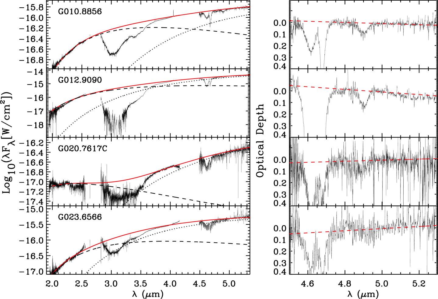
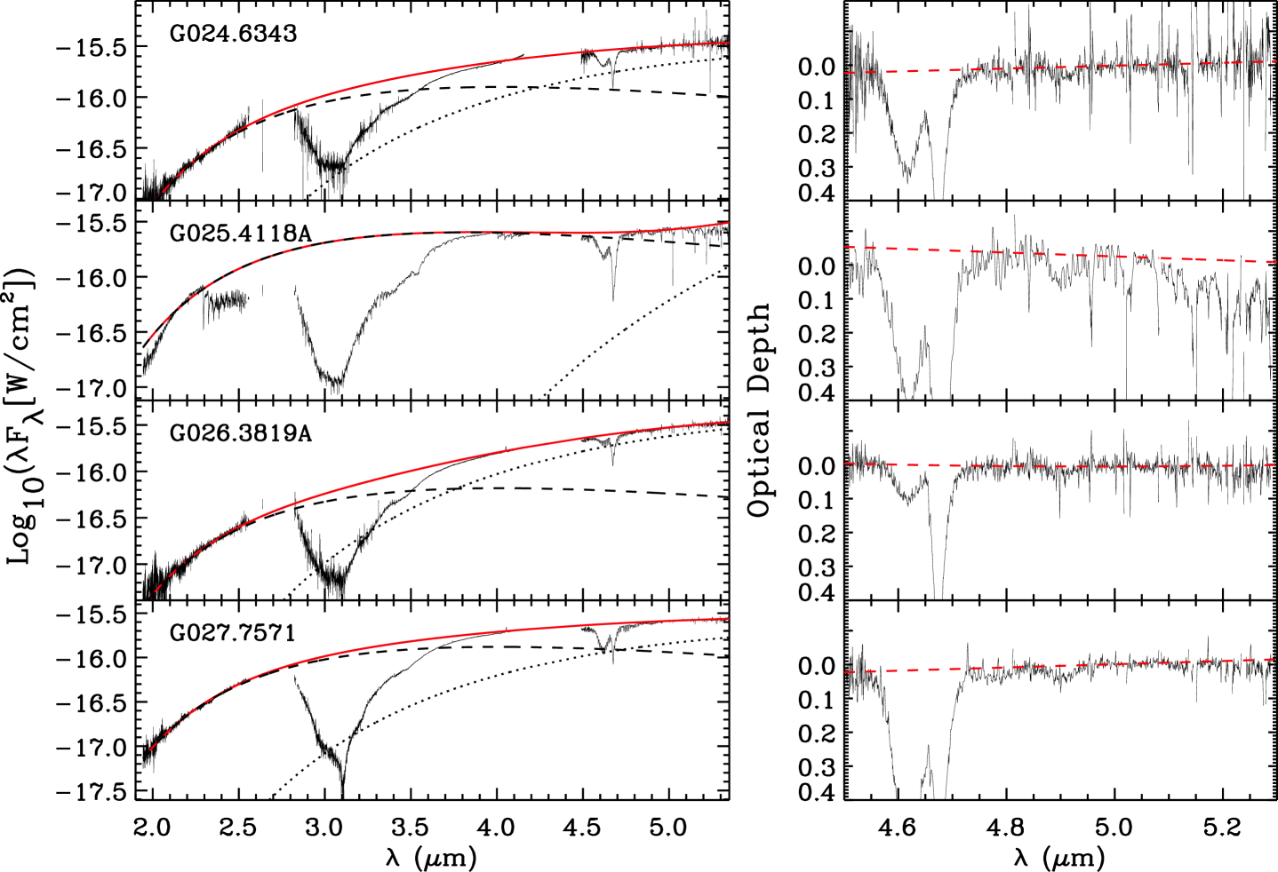
Figure 1: IRTF/SpeX spectra of MYSO sample. The left panels show the flux spectra with the Rayleigh-Jeans continuum of a hot star (dashed) and a blackbody continuum spectrum of warm dust (dotted), both reddened by the same amount of foreground extinction. The sum of the two components, indicated by the red line, is used to put the spectra on optical depth scale. The right panels zoom in on the $M$-band spectrum, on optical depth scale. A local baseline is indicated with the dashed red line, which is subtracted before the OCN^-, CO, and OCS ice absorption features are analyzed.

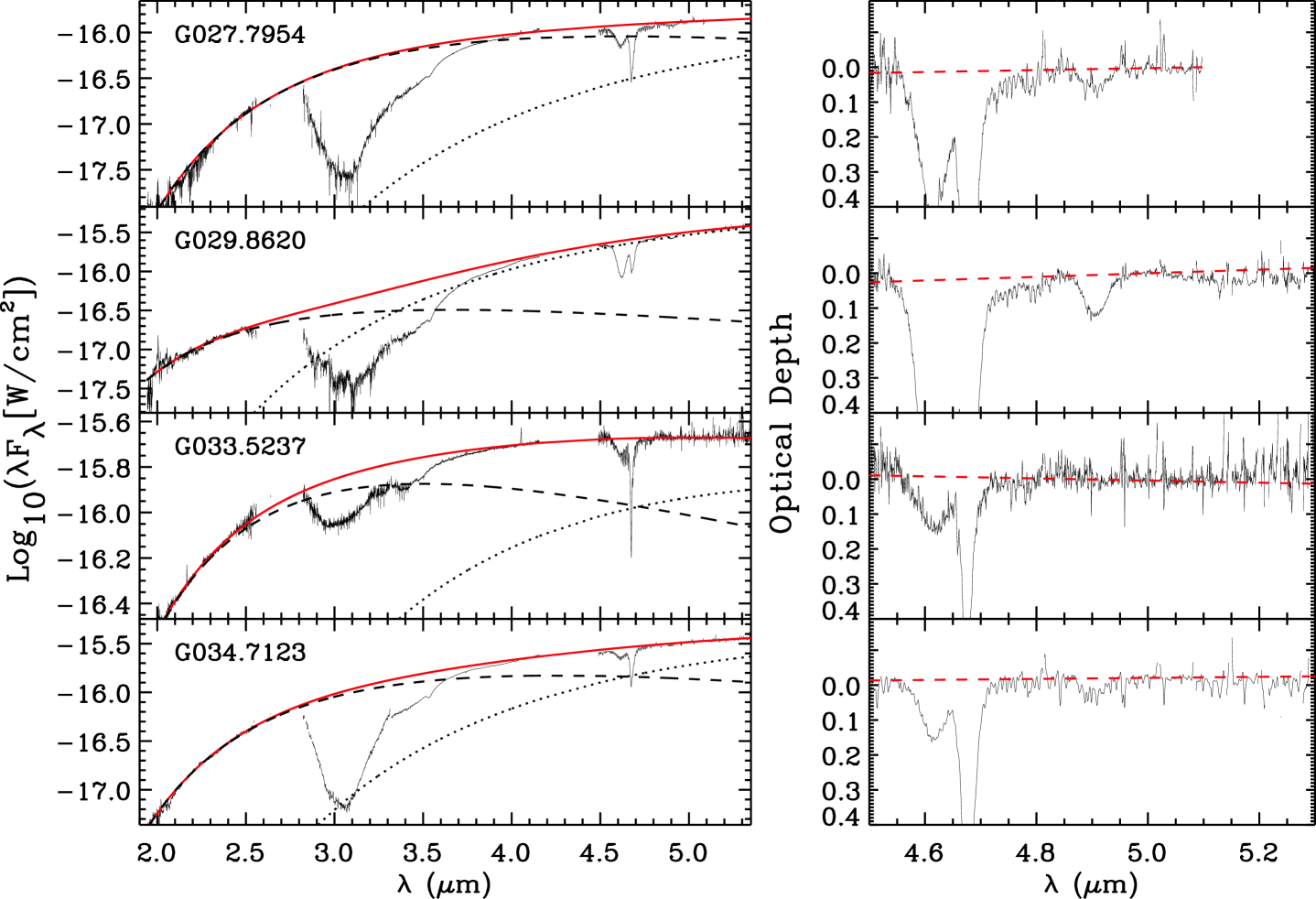
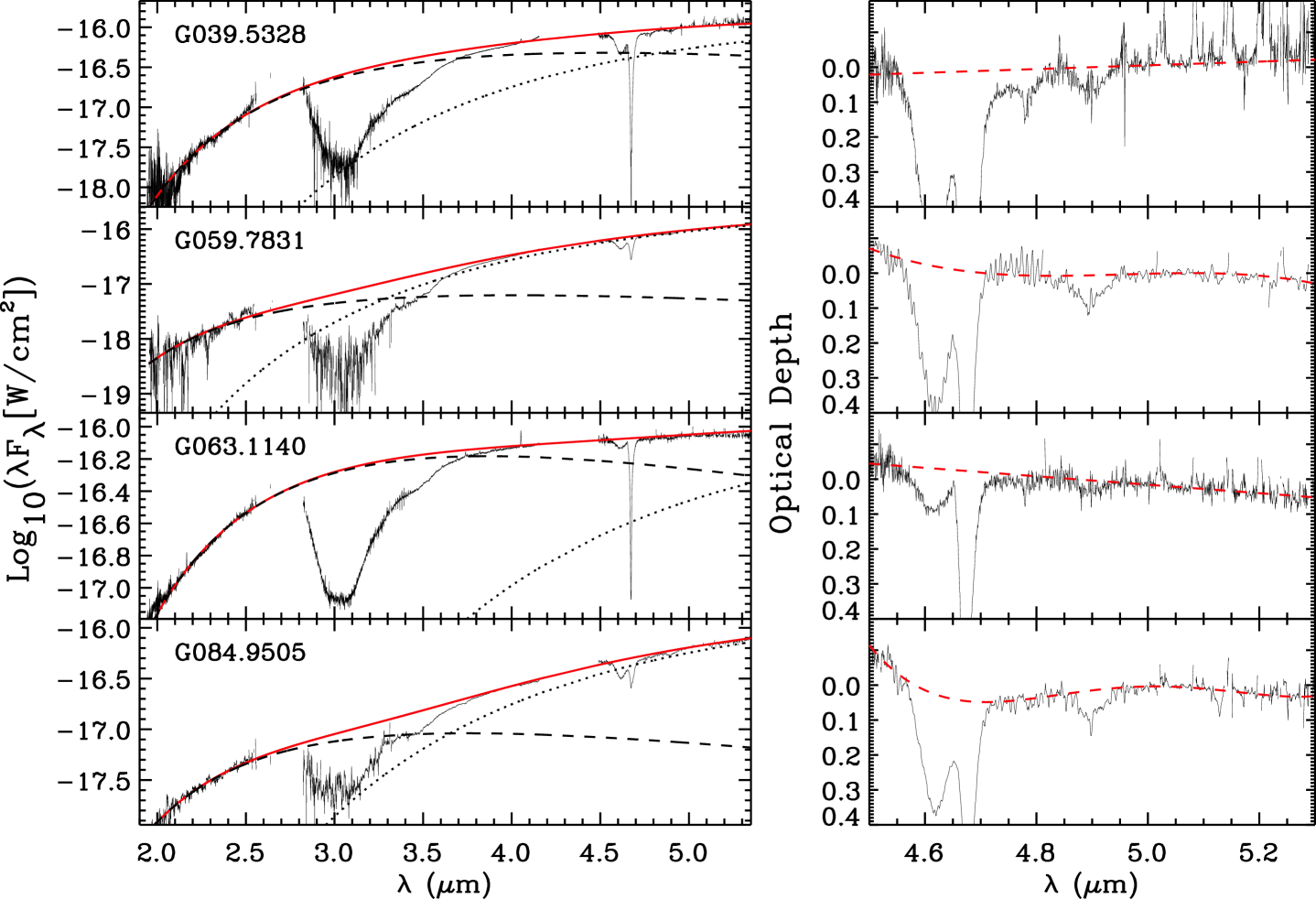
Figure 2: IRTF/SpeX spectra of MYSO sample. For more details, see the caption of Figure 1.

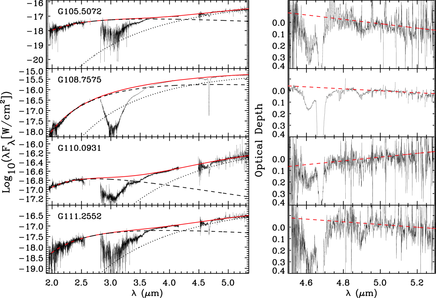
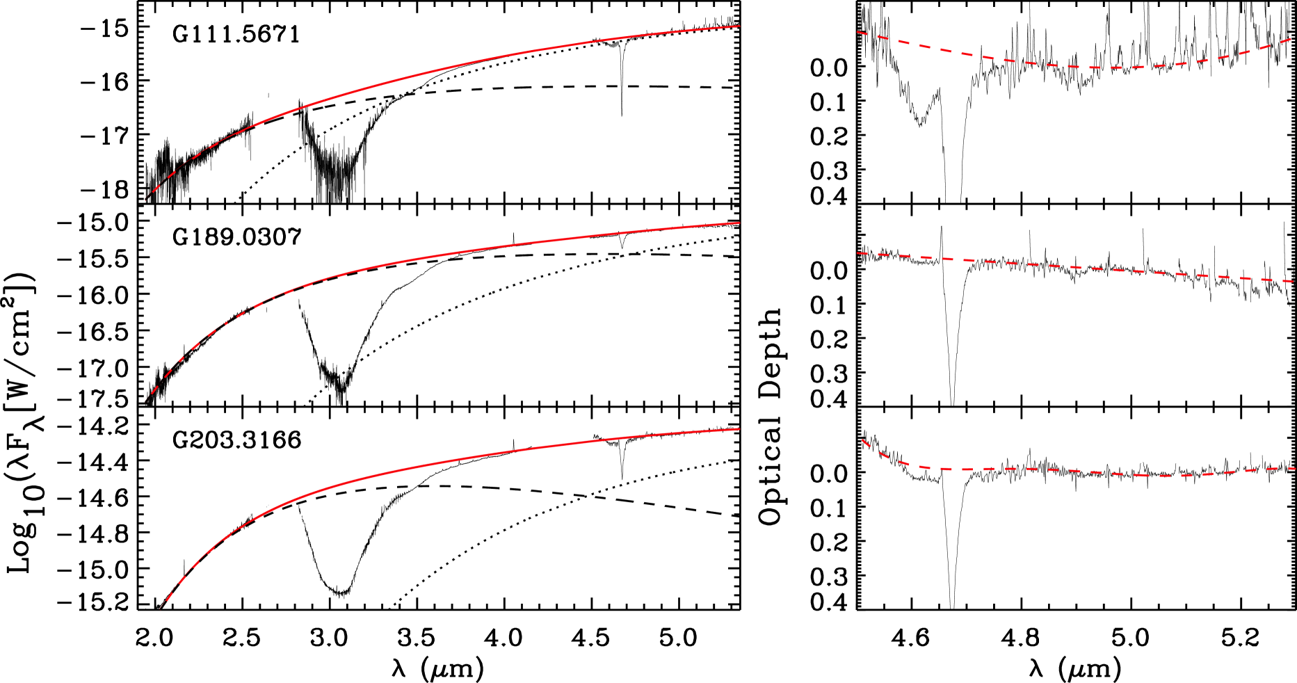
Figure 3: IRTF/SpeX spectra of MYSO sample. For more details, see the caption of Figure 1.

Figure 4: IRTF/SpeX spectrum of the MYSO G012.9090-00.2607 (W33A; black solid line) compared to a space based ISO/SWS spectrum across the full wavelength range (red; Gibb et al. 2004). The IRTF/SpeX and ISO/SWS spectra are overall in good agreement, showing the same absorption features and continuum shape. The dotted line indicates the continuum level described in §4.1 and Figs. 1-3. The dashed line is the continuum level including absorption by H₂O ice, showing the effect of the broad $\sim$4.5 ${\rm\mu m}$ H₂O combination mode. A change in slope is visible near $\sim$5.0 ${\rm\mu m}$ in both the IRTF/SpeX and ISO/SWS spectra, due to what appears to be a shallow absorption feature centered on $\sim$5.25 ${\rm\mu m}$. The change in slope at $\sim$ 5.5 ${\rm\mu m}$ is due to the onset of the prominent 6.0 ${\rm\mu m}$ absorption band. The apparent lack of absorption by gas phase CO lines in the ISO/SWS spectrum is due to its low spectral resolving power ($R=800$ versus $R=$1,500).

4.1 Continuum Determination

To be able to analyze the profile and depth of the ice absorption features, a global baseline defining the continuum emission was determined over the full observed wavelength range of 1.95-5.36 ${\rm\mu m}$. This baseline was determined by fitting a simple model of two reddened blackbody functions to the data. The first blackbody is that from a hot central source. Its temperature is assumed to be at least several tens of thousand Kelvin, so that it is represented by a temperature-independent Rayleigh-Jeans tail in the observed wavelength range. The second blackbody represents the emission by warm dust along the line of sight, perhaps from a circumstellar disk or the inner envelope. Both blackbodies are reddened by the same foreground extinction due to cooler envelope and foreground cloud material. The extinction curve used for this is that derived for the J, H, and K-bands by Indebetouw et al. (2005), and at longer wavelengths it is assumed to be flat. Furthermore, the 3.0 ${\rm\mu m}$ ice band was also included in the model, because H₂O absorption covers such a large portion of the observed wavelength range. For this, we used template 3.0 ${\rm\mu m}$ band spectra derived from previously well studied MYSOs (Gibb et al., 2004), covering a range of profiles (AFGL 2136, MonR2 IRS3, AFGL 989, NGC 7538 IRS9, S140 IRS1). This model thus contains four variables: the temperature of the warm dust emission, the foreground extinction $A_{\rm V}$, the peak optical depth of the 3.0 ${\rm\mu m}$ ice band $\tau_{3.0}$, and a relative flux scaling factor for the hot (Rayleigh-Jeans) and warm blackbody emission. This model is then normalized to the observed spectrum near 5 ${\rm\mu m}$ and fitted to selected wavelength ranges. Those ranges avoid the long-wavelength wing of the 3.0 ${\rm\mu m}$ ice band ($\sim$ 3.2-3.9 ${\rm\mu m}$), the OCN^-, CO, and OCS ice features (4.5-4.9 ${\rm\mu m}$), as well as regions with poor atmospheric transmission.

The global baseline model generally fits the observations well (Figs. 1-3). The spectra were subsequently converted to optical depth scale. At a detailed level in the $M$-band optical depth spectra, small offsets from the zero optical depth level were observed, however, and these were removed by subtracting an additional local straight line fit, shown in Figs. 1-3.

Because it is our primary goal to determine the baseline for the ice features, we do not present or further interpret the parameters and their uncertainties for the blackbody fit parameters. Due to the small width of the ice features in the $M$-band, and the subtraction of an additional local baseline, the uncertainty due to the baseline is small. An error of 0.01 is included in the uncertainties derived for the ice band optical depths. Uncertainties for the 3.0 ${\rm\mu m}$ H₂O ice band optical depths are larger ($\sim 10\%$). This was checked by using a different method to determine the baseline for the 3.0 $\mu$m band, applying a spline function (K. Emerson et al., in preparation). These uncertainties are included in the derived H₂O ice column densities (§4.3.5).

4.2 Gas Phase CO

Many targets show absorption, and some emission, by the ro-vibrational lines of gas phase ¹²CO, and sometimes ¹³CO. These lines are unresolved at the IRTF/SpeX resolving power of $R=1,500-2,500$. At the level of a few percent of the continuum, these lines somewhat affect the profiles of the ice absorption features. We therefore attempt to remove them using a rotation diagram analysis (Fig. 5). Integrated absorption line depths were measured, and converted to lower level column densities assuming optically thin absorption in Local Thermodynamic Equilibrium (LTE). The constructed rotation diagrams typically show a steep linear relation at low energy levels, and a shallower linear relation at higher energy levels. Straight lines were fitted to each of these, providing integrated line depths for all rotational levels. These were then used to divide out the gas phase CO lines. The detected ¹²CO lines are most likely optically thick, and we do not further use the column densities and excitation temperatures, derived from the rotation diagrams in the optically thin limit, in this paper.

Figure 5: Illustration of the removal of gas phase ¹²CO ro-vibrational absorption lines for the MYSO G108.7575$-$00.9863. Panel a is the IRTF/SpeX spectrum before removal, and panel b after. Panel c shows the rotation diagram used in this process, with $E_{\rm low}$, $N_{\rm low}$, and $J_{\rm low}$ the energy level, column density, and rotational quantum number for the lower energy levels, respectively. Two slope regimes are discerned, which are fitted with two straight lines, corresponding to excitation temperatures of 90 and 895 K and column densities of 7.5$\times 10^{16}$ and 2.5$\times 10^{17}$ ${\rm cm^{-2}}$, respectively. These temperatures are likely highly inaccurate, and the column densities strongly underestimated due to the lines being optically thick.

4.3 Ice Band Profiles and Column Densities

The absorption features detected at $\sim$4.62, 4.67, and 4.90 ${\rm\mu m}$ are shown in Figures 6-8 on optical depth scale. They are ascribed to OCN^-, CO, and OCS, respectively, and are fitted with Gaussian and Lorentzian functions to characterize their profiles and depths. To put the results in an astrochemical context, the 3.0 and 3.53 ${\rm\mu m}$ absorption bands of H₂O and CH₃OH ice are discussed as well. However, for a more detailed analysis of these two bands, in a much larger sample of MYSOs, we refer to K. Emerson et al. (in preparation).

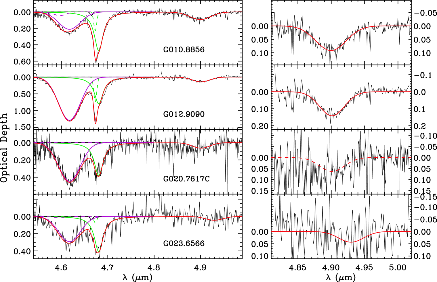
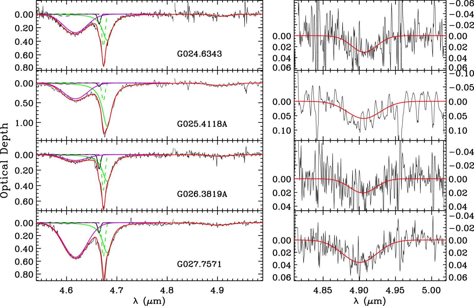
Figure 6: $M$-band spectra of the MYSO sample on optical depth scale. A zoom in on the OCS ice band is shown in the right panels. The OCS band is fitted with a single Gaussian. To this are added the Gaussian and Lorentzian fits to the CO ice bands (green and black, respectively) and Gausian fits to the 2165.7 and 2175.4 ${\rm cm^{-1}}$ components of the OCN^- band (solid purple and dashed purple, respectively). A dashed red line in the right panels indicates that OCS was not detected and the Gaussian depth should be regarded as an upper limit.

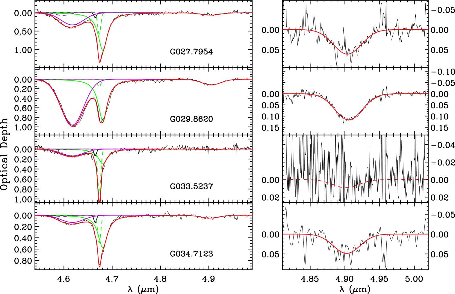
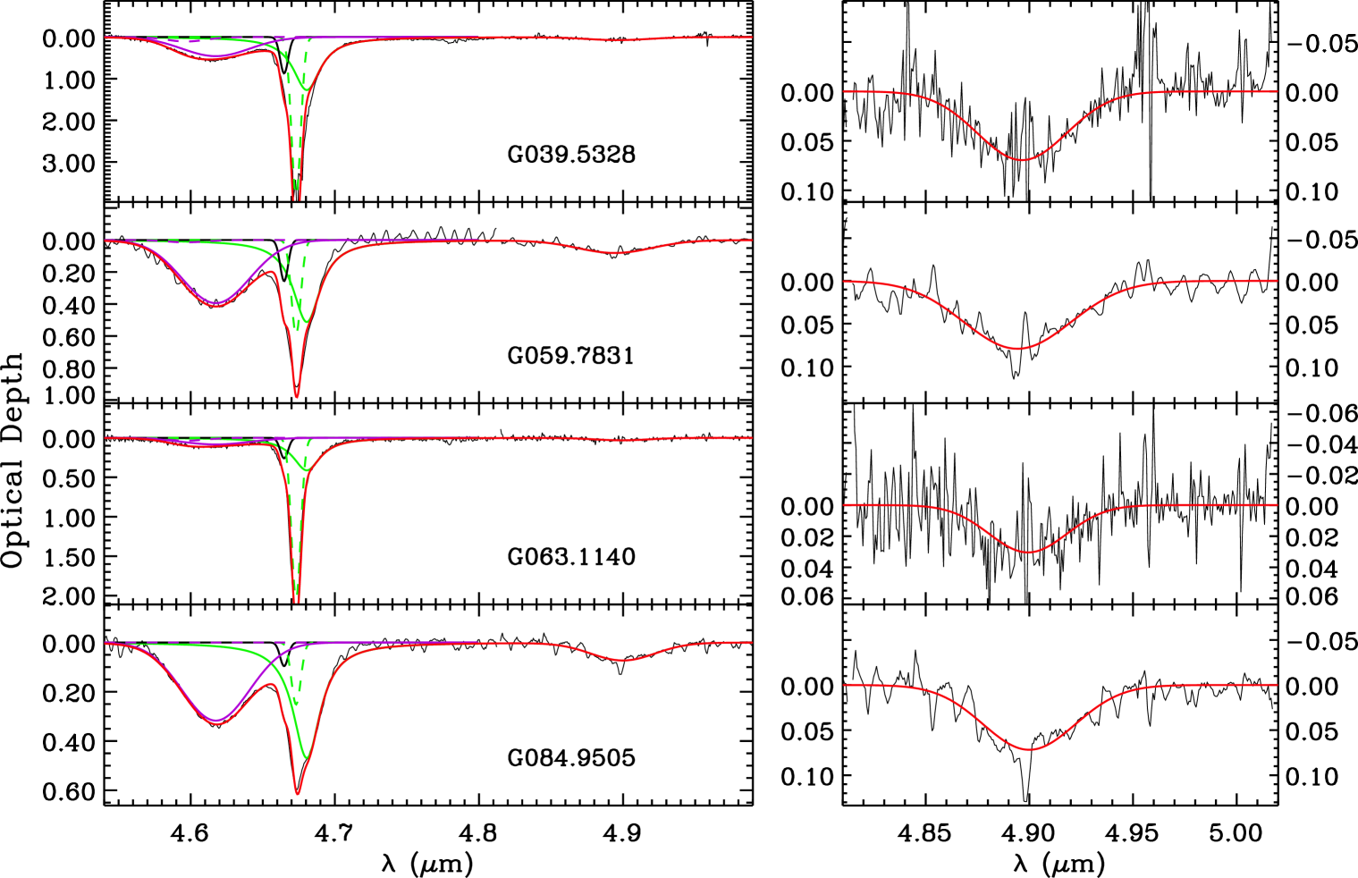
Figure 7: $M$-band spectra of the MYSO sample on optical depth scale. For more details, see the caption of Figure 6.

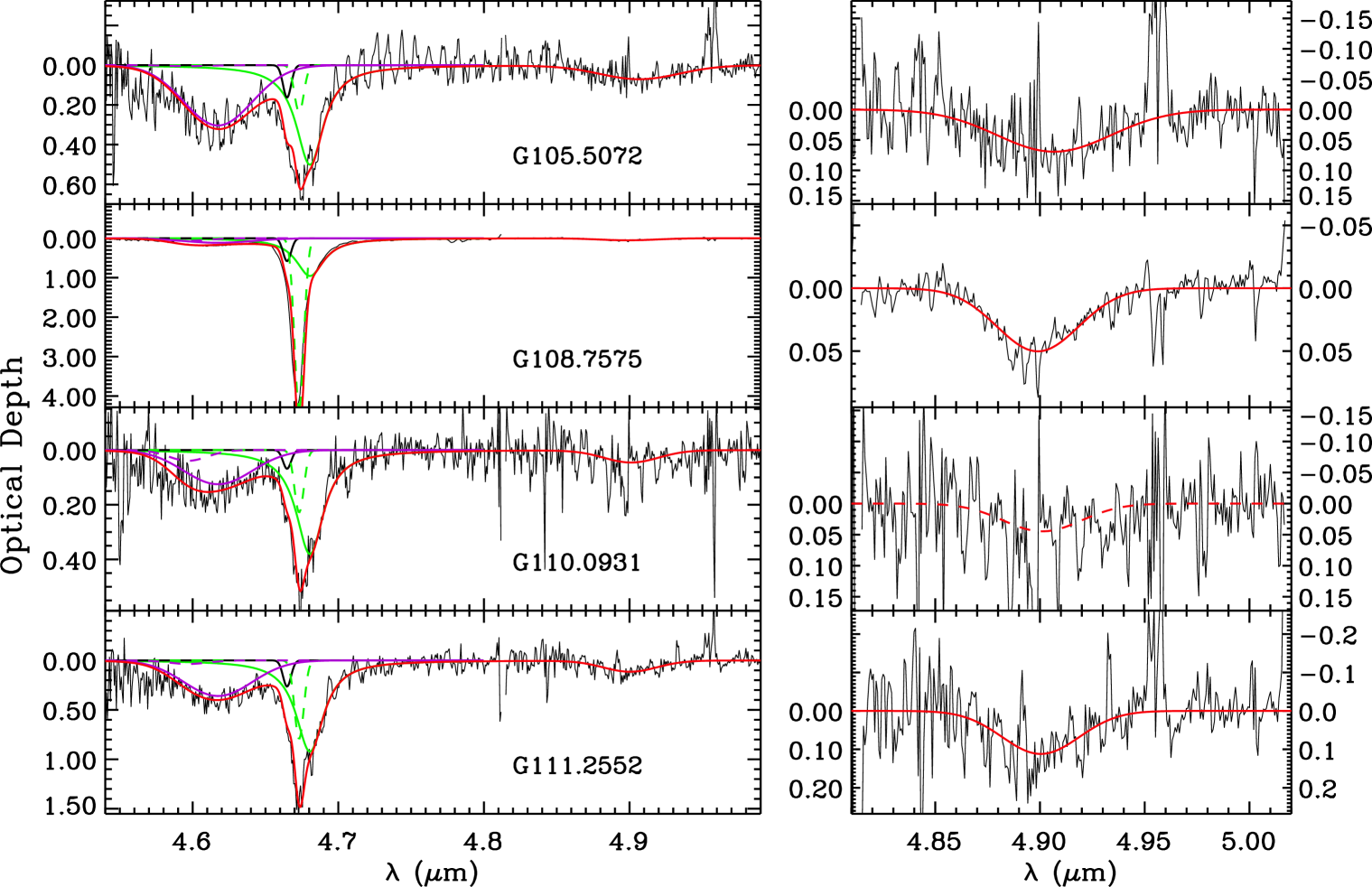
Figure 8: $M$-band spectra of the MYSO sample on optical depth scale. For more details, see the caption of Figure 6.

4.3.1 CO

The 4.67 ${\rm\mu m}$ absorption band of CO ice shows significant profile variations (Figs. 6-8). For some targets the profile is much narrower (e.g., G063.1140) than for others (e.g., G025.4118A). Such variations were previously observed for both high and low mass YSOs, and were ascribed to the presence of CO in different molecular environments (Tielens et al., 1991; Boogert et al., 2002; Pontoppidan et al., 2003): a central, narrow absorption due to pure CO (and traces of other low dipole moment molecules), a broad red-shifted absorption due to CO mixed with high dipole moment species (H₂O, CH₃OH), and a minor blue-shifted absorption, likely due to CO mixed wth CO₂ ice. By fitting constant profiles for CO_apolar, CO_polar, and CO_blue, and only varying the peak optical depths, good fits are obtained across a wide range of low and high mass YSOs as well as background stars (Pontoppidan et al., 2003). The same approach is adopted for the MYSOs in this work. CO_apolar was fitted using a Gaussian function (peak wavelength 4.6731 ${\rm\mu m}$, FWHM=0.0076 ${\rm\mu m}$), CO_polar with a Lorentzian (4.6806 and 0.0232 ${\rm\mu m}$), and CO_blue with a Gaussian (4.6648 and 0.0065 ${\rm\mu m}$). The fitting process was done simultaneously with the 4.62 ${\rm\mu m}$ band of OCN^- (§4.3.2), due to the wavelength overlap. Also, all components were convolved with the Gaussian SpeX instrument profile before fitting them to the data. Satisfactory fits are obtained for all bands (Figs. 6-8). The total CO ice column densities and those of the different components are listed in Table 2. An integrated band strength of 1.1$\times 10^{-17}$ cm/molecule, as measured in the laboratory (Jiang et al., 1975), was used for this.

Table 2: H₂O and CO Ice Column Densities 

Source	$N$(H2O)	$N$(CO)		$N$(COapolar)	$N$(COpolar)	$N$(COblue)
MSX	$10^{18}$ cm-2	$10^{17}$ cm-2	% H2O	$10^{17}$ cm-2	$10^{17}$ cm-2	$10^{17}$ cm-2
G010.8856$+$00.1221	1.75 (0.10)	5.40 (0.27)	30.86 (2.29)	0.72 (0.11)	4.56 (0.22)	0.12 (0.10)
G012.9090$-$00.2607	11.50 (1.29)	9.97 (0.40)	8.67 (1.03)	2.32 (0.17)	7.65 (0.33)	0.00 (0.15)
G020.7617$-$00.0638C	$\sim$ 1.15	3.73 (0.55)	$\sim$32.43	0.08 (0.23)	3.65 (0.44)	0.00 (0.22)
G023.6566$-$00.1273	1.76 (0.15)	4.27 (0.51)	24.26 (3.52)	0.23 (0.22)	3.92 (0.42)	0.11 (0.20)
G024.6343$-$00.3233	2.69 (0.18)	5.62 (0.26)	20.89 (1.69)	1.50 (0.11)	3.72 (0.22)	0.40 (0.09)
G025.4118$+$00.1052A	4.88 (0.32)	12.20 (0.32)	25.00 (1.78)	1.43 (0.13)	10.50 (0.27)	0.24 (0.12)
G026.3819$+$01.4057A	3.62 (0.32)	5.29 (0.27)	14.61 (1.50)	1.45 (0.11)	3.34 (0.22)	0.50 (0.10)
G027.7571$+$00.0500	4.22 (0.42)	6.63 (0.30)	15.71 (1.73)	1.68 (0.12)	4.53 (0.25)	0.42 (0.11)
G027.7954$-$00.2772	4.32 (0.28)	12.00 (0.30)	27.78 (1.94)	1.83 (0.12)	9.82 (0.25)	0.36 (0.11)
G029.8620$-$00.0444	4.08 (0.82)	8.88 (0.29)	21.76 (4.41)	0.54 (0.12)	8.34 (0.25)	0.00 (0.11)
G033.5237$+$00.0198	0.76 (0.08)	6.04 (0.31)	79.68 (9.39)	2.82 (0.13)	2.85 (0.26)	0.36 (0.11)
G034.7123$-$00.5946	4.22 (0.24)	7.46 (0.27)	17.68 (1.20)	1.55 (0.11)	5.56 (0.23)	0.35 (0.10)
G039.5328$-$00.1969	4.26 (0.40)	26.70 (1.77)	62.68 (7.25)	12.10 (0.77)	12.30 (1.42)	2.37 (0.72)
G059.7831$+$00.0648	5.81 (1.29)	7.51 (0.38)	12.93 (2.94)	1.87 (0.15)	4.94 (0.31)	0.70 (0.15)
G063.1140$+$00.3416	3.02 (0.18)	11.10 (0.32)	36.75 (2.41)	6.43 (0.13)	3.97 (0.27)	0.71 (0.12)
G084.9505$-$00.6910	2.32 (0.40)	5.58 (0.23)	24.05 (4.30)	0.80 (0.09)	4.52 (0.19)	0.26 (0.08)
G105.5072$+$00.2294	4.44 (1.13)	6.02 (0.54)	13.56 (3.66)	0.75 (0.22)	4.83 (0.44)	0.44 (0.21)
G108.7575$-$00.9863	6.28 (0.48)	24.50 (1.24)	39.01 (3.60)	13.70 (0.56)	9.23 (0.99)	1.58 (0.50)
G110.0931$-$00.0641	1.73 (0.24)	4.57 (0.42)	26.42 (4.42)	0.72 (0.18)	3.66 (0.34)	0.19 (0.16)
G111.2552$-$00.7702	$\sim$ 4.56	12.10 (0.68)	$\sim$26.54	2.51 (0.28)	8.88 (0.55)	0.72 (0.28)
G111.5671$+$00.7517	5.37 (0.48)	16.20 (0.36)	30.17 (2.80)	8.60 (0.15)	6.97 (0.30)	0.63 (0.13)
G189.0307$+$00.7821	5.46 (0.48)	3.68 (0.31)	6.74 (0.82)	1.13 (0.13)	2.06 (0.26)	0.49 (0.11)
G203.3166$+$02.0564	2.24 (0.11)	3.72 (0.23)	16.61 (1.32)	1.18 (0.09)	2.04 (0.20)	0.51 (0.08)

Note. — Values in brackets indicate 1$\sigma$ uncertainties.

4.3.2 OCN^-

The 4.62 ${\rm\mu m}$ band of OCN^- was detected toward all targets. In a study of low and high mass YSOs, it was found that this band consists of two components, centered on 2165.7 and 2175.4 ${\rm cm^{-1}}$ (4.6174 and 4.5969 ${\rm\mu m}$; van Broekhuizen et al. 2005). The 2165.7 ${\rm cm^{-1}}$ component was found to be consistent with solid OCN^- in polar environments, while the other component relates perhaps to CO bonding to the grain surfaces or to OCN^- in apolar environments (Öberg et al., 2011). We adopt the same decomposition procedure, by fitting two Gaussians, one at 2165.7 ${\rm cm^{-1}}$ ($FWHM=$26 ${\rm cm^{-1}}$) and one at 2175.4 ${\rm cm^{-1}}$ ($FWHM=$15 ${\rm cm^{-1}}$). The fitting was done simultaneously with those of the CO ice feature (§4.3.1), since they overlap. Good quality fits were obtained (Figs. 6-8). The contribution by the 2175.4 ${\rm cm^{-1}}$ component is usually at the less than 2$\sigma$ confidence level, except for three targets at 2-3$\sigma$, and three targets at $>3\sigma$. The OCN^- column densities are listed in Table 3. An integrated band strength of 1.3$\times 10^{-16}$ cm/molecule, as measured in the laboratory (van Broekhuizen et al., 2004), was used for this.

Table 3: OCN^- and CH₃OH Ice Column Densities 

Source	$N$(OCN${}^{-}_{\rm red}$)		$N$(OCN${}^{-}_{\rm blue}$)		$N$(CH3OH)
MSX	$10^{16}$ cm-2	% H2O	$10^{16}$ cm-2	% H2O	$10^{16}$ cm-2	% H2O
G010.8856$+$00.1221	4.24 (0.35)	2.42 (0.24)	0.52 (0.23)	0.30 (0.13)	60.2 (13.5)	34.4 ( 7.9)
G012.9090$-$00.2607	25.70 (0.37)	2.23 (0.25)	0.00 (0.24)	0.00 (0.02)	235.0 (52.6)	20.4 ( 5.1)
G020.7617$-$00.0638C	8.93 (0.67)	$\sim$ 7.77	0.00 (0.47)	$\sim$ 0.00	$<$115.0	$<$100.0
G023.6566$-$00.1273	5.85 (0.63)	3.32 (0.45)	0.20 (0.44)	0.11 (0.25)	37.3 ( 8.3)	21.2 ( 5.0)
G024.6343$-$00.3233	5.45 (0.36)	2.03 (0.19)	0.35 (0.24)	0.13 (0.09)	$<$ 22.9	$<$ 8.5
G025.4118$+$00.1052A	8.03 (0.41)	1.65 (0.14)	0.38 (0.28)	0.08 (0.06)	138.0 (30.8)	28.3 ( 6.6)
G026.3819$+$01.4057A	1.50 (0.31)	0.41 (0.09)	0.12 (0.20)	0.03 (0.06)	27.3 ( 6.1)	7.5 ( 1.8)
G027.7571$+$00.0500	10.80 (0.34)	2.56 (0.27)	0.22 (0.22)	0.05 (0.05)	$<$ 15.5	$<$ 3.7
G027.7954$-$00.2772	6.61 (0.35)	1.53 (0.13)	0.86 (0.23)	0.20 (0.06)	87.1 (19.5)	20.2 ( 4.7)
G029.8620$-$00.0444	19.20 (0.35)	4.71 (0.95)	0.00 (0.23)	0.00 (0.06)	165.0 (36.8)	40.4 (12.1)
G033.5237$+$00.0198	2.75 (0.34)	3.63 (0.59)	0.12 (0.22)	0.16 (0.29)	$<$ 11.5	$<$ 15.2
G034.7123$-$00.5946	2.56 (0.29)	0.61 (0.08)	0.28 (0.18)	0.07 (0.04)	110.0 (24.7)	26.1 ( 6.0)
G039.5328$-$00.1969	9.19 (0.36)	2.16 (0.22)	1.24 (0.23)	0.29 (0.06)	32.0 ( 7.1)	7.5 ( 1.8)
G059.7831$+$00.0648	7.89 (0.34)	1.36 (0.31)	0.16 (0.22)	0.03 (0.04)	137.0 (30.5)	23.6 ( 7.4)
G063.1140$+$00.3416	1.69 (0.30)	0.56 (0.10)	0.42 (0.19)	0.14 (0.06)	34.4 ( 7.7)	11.4 ( 2.6)
G084.9505$-$00.6910	6.34 (0.29)	2.73 (0.49)	0.00 (0.18)	0.00 (0.08)	$<$ 28.7	$<$ 12.4
G105.5072$+$00.2294	6.08 (0.78)	1.37 (0.39)	0.06 (0.56)	0.01 (0.13)	$<$ 45.9	$<$ 10.3
G108.7575$-$00.9863	2.33 (0.34)	0.37 (0.06)	0.79 (0.22)	0.13 (0.04)	64.9 (14.5)	10.3 ( 2.4)
G110.0931$-$00.0641	2.50 (0.76)	1.45 (0.48)	0.45 (0.54)	0.26 (0.31)	$<$ 23.7	$<$ 13.7
G111.2552$-$00.7702	7.19 (0.98)	$\sim$ 1.58	0.41 (0.71)	$\sim$ 0.09	149.0 (33.3)	$\sim$ 32.7
G111.5671$+$00.7517	3.41 (0.39)	0.64 (0.09)	0.60 (0.26)	0.11 (0.05)	43.0 ( 9.6)	8.0 ( 1.9)
G189.0307$+$00.7821	0.20 (0.25)	0.04 (0.05)	0.00 (0.15)	0.00 (0.03)	39.2 ( 8.8)	7.2 ( 1.7)
G203.3166$+$02.0564	0.49 (0.27)	0.22 (0.12)	0.10 (0.17)	0.04 (0.07)	$<$ 14.3	$<$ 6.4

Note. — Values in brackets indicate 1$\sigma$ uncertainties.

4.3.3 OCS

The absorption feature at 4.90 ${\rm\mu m}$, attributed to the C-O stretch mode of solid OCS, is well fitted with a single Gaussian for all MYSOs (Figs. 6-8). Upper limits are derived for three of the targets. The fit parameters are listed in Table 4. Solid OCS column densities were derived using an integrated band strength of 1.5$\times 10^{-16}$ cm/molecule, as measured in the laboratory (Palumbo et al., 1997). In order to highlight similarities and differences among the targets, each target is compared to the same Gaussian in Figure 9. Clearly, any profile variations are small.

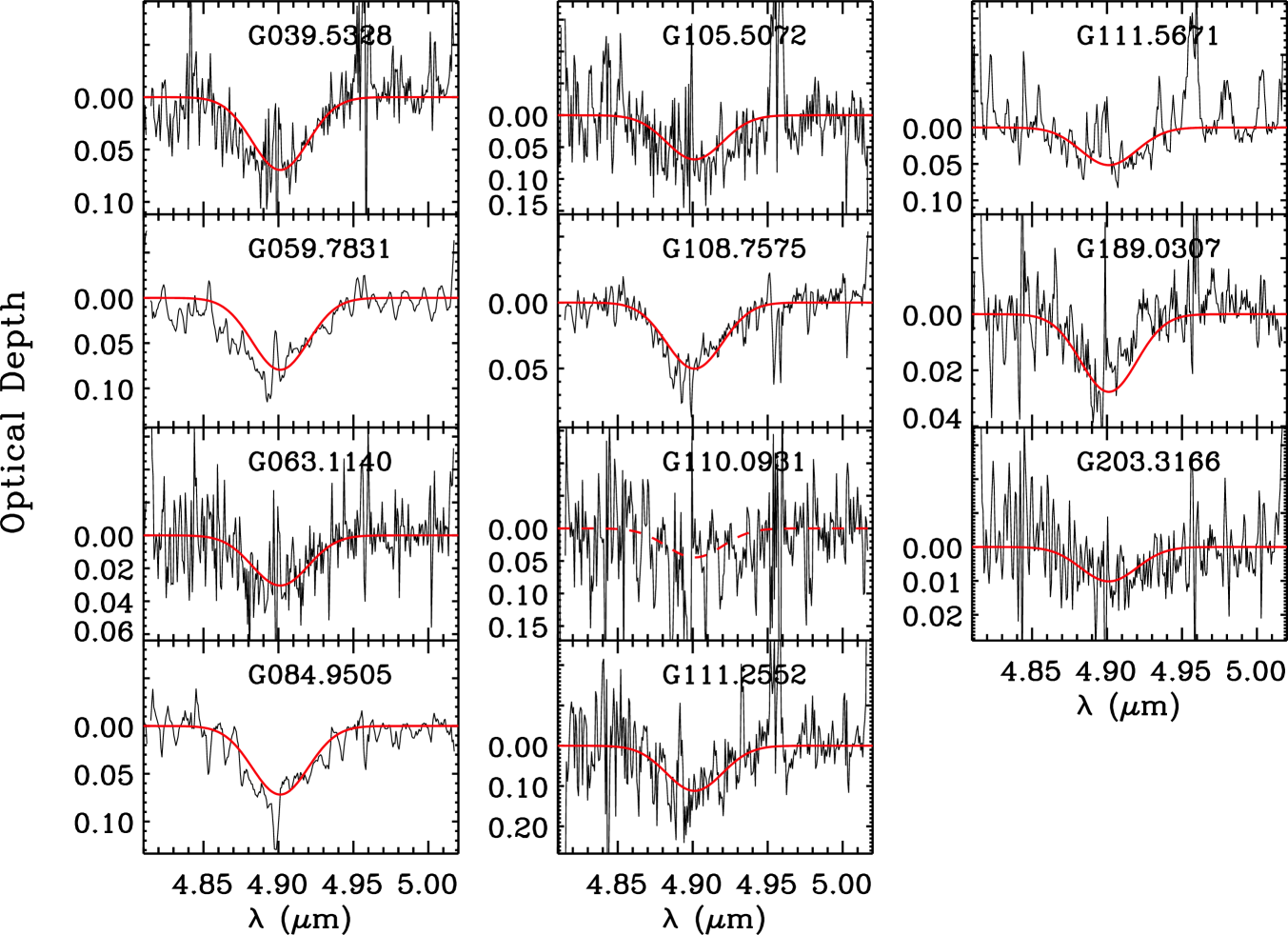
Figure 9: The OCS ice band towards the sample of MYSOs compared to the same Gaussian, scaled to the best-fit peak optical depth of Table 4 in order to highlight any variations in the sample. The Gaussian represents the best fit to the target G012.9090 (W33A; $\lambda=$4.9012 ${\rm\mu m}$, FWHM=0.0441 ${\rm\mu m}$).

Table 4: OCS Band Parameters and Column Densities 

Source	$\lambda_{\rm peak}$		FWHM		$\tau_{\rm peak}$	$N$(OCS)
MSX	$\mu$m	cm-1	$\mu$m	cm-1		$10^{16}$ cm-2	% H2O
G010.8856$+$00.1221	4.8996 (0.0008)	2041.0 (0.4)	0.0535 (0.0017)	22.3 (0.7)	0.092 (0.000)	1.37 (0.04)	0.78 (0.05)
G012.9090$-$00.2607	4.9012 (0.0016)	2040.3 (0.7)	0.0441 (0.0034)	18.4 (1.4)	0.142 (0.002)	1.74 (0.13)	0.15 (0.02)
G020.7617$-$00.0638C	…	…	…	…	…	$<$ 0.78	$<$ 0.68
G023.6566$-$00.1273	4.9297 (0.0072)	2028.5 (3.0)	0.0442 (0.0159)	18.2 (6.6)	0.044 (0.002)	0.53 (0.19)	0.30 (0.11)
G024.6343$-$00.3233	4.9068 (0.0079)	2038.0 (3.3)	0.0417 (0.0163)	17.3 (6.8)	0.030 (0.002)	0.35 (0.14)	0.13 (0.05)
G025.4118$+$00.1052A	4.9061 (0.0032)	2038.3 (1.3)	0.0542 (0.0069)	22.5 (2.9)	0.060 (0.001)	0.89 (0.12)	0.18 (0.03)
G026.3819$+$01.4057A	4.9048 (0.0030)	2038.8 (1.2)	0.0426 (0.0060)	17.7 (2.5)	0.021 (0.000)	0.24 (0.03)	0.07 (0.01)
G027.7571$+$00.0500	4.9005 (0.0038)	2040.6 (1.6)	0.0562 (0.0081)	23.4 (3.4)	0.036 (0.001)	0.57 (0.08)	0.13 (0.02)
G027.7954$-$00.2772	4.9035 (0.0006)	2039.4 (0.3)	0.0475 (0.0013)	19.8 (0.5)	0.061 (0.000)	0.80 (0.02)	0.19 (0.01)
G029.8620$-$00.0444	4.9053 (0.0003)	2038.6 (0.1)	0.0465 (0.0005)	19.3 (0.2)	0.117 (0.000)	1.50 (0.02)	0.37 (0.07)
G033.5237$+$00.0198	…	…	…	…	…	$<$ 0.11	$<$ 0.15
G034.7123$-$00.5946	4.9025 (0.0024)	2039.8 (1.0)	0.0454 (0.0051)	18.9 (2.1)	0.049 (0.001)	0.61 (0.07)	0.14 (0.02)
G039.5328$-$00.1969	4.8965 (0.0026)	2042.3 (1.1)	0.0508 (0.0054)	21.2 (2.3)	0.069 (0.001)	0.98 (0.11)	0.23 (0.03)
G059.7831$+$00.0648	4.8943 (0.0012)	2043.2 (0.5)	0.0609 (0.0025)	25.4 (1.1)	0.079 (0.001)	1.34 (0.06)	0.23 (0.05)
G063.1140$+$00.3416	4.8994 (0.0044)	2041.1 (1.9)	0.0442 (0.0091)	18.4 (3.8)	0.030 (0.001)	0.37 (0.08)	0.12 (0.03)
G084.9505$-$00.6910	4.8999 (0.0005)	2040.8 (0.2)	0.0523 (0.0011)	21.8 (0.5)	0.072 (0.000)	1.04 (0.02)	0.45 (0.08)
G105.5072$+$00.2294	4.9067 (0.0117)	2038.0 (4.9)	0.0641 (0.0259)	26.6 (10.8)	0.069 (0.004)	1.23 (0.50)	0.28 (0.13)
G108.7575$-$00.9863	4.8990 (0.0010)	2041.2 (0.4)	0.0460 (0.0019)	19.2 (0.8)	0.050 (0.000)	0.64 (0.03)	0.10 (0.01)
G110.0931$-$00.0641	…	…	…	…	…	$<$ 0.55	$<$ 0.32
G111.2552$-$00.7702	4.9004 (0.0063)	2040.7 (2.6)	0.0434 (0.0128)	18.1 (5.3)	0.112 (0.006)	1.35 (0.40)	$\sim$ 0.30
G111.5671$+$00.7517	4.9055 (0.0022)	2038.5 (0.9)	0.0508 (0.0046)	21.1 (1.9)	0.052 (0.001)	0.73 (0.07)	0.14 (0.02)
G189.0307$+$00.7821	4.8953 (0.0011)	2042.8 (0.5)	0.0292 (0.0021)	12.2 (0.9)	0.028 (0.000)	0.22 (0.02)	0.04 (0.00)
G203.3166$+$02.0564	4.9103 (0.0048)	2036.5 (2.0)	0.0477 (0.0098)	19.8 (4.1)	0.010 (0.000)	0.13 (0.03)	0.06 (0.01)

4.3.4 CH₃OH

To put the OCS, OCN^-, and CO observations in an astrochemical context, CH₃OH ice column densities were derived as well. The 3.53 ${\rm\mu m}$ C-H stretch mode of solid CH₃OH is detected towards 15 of the 23 MYSOs. As shown in Figures 10-12, the CH₃OH band overlaps with the 3.47 ${\rm\mu m}$ absorption feature, which is possibly due to NH₃ hydrates (Dartois & d’Hendecourt, 2001). These absorption features are located on the wing of the deep 3.0 ${\rm\mu m}$ band of H₂O ice. A low order polynomial was used to define and subtract a local baseline. The absorption features were then disentangled by fitting the combination of a Gaussian and a laboratory spectrum. The laboratory spectrum used is the mixture H₂O:CH₃OH:CO:NH₃=100:50:1:1 at a temperature of 10 K (Hudgins et al., 1993). To provide more stable solutions, the Gaussian peak position and $FWHM$ were kept fixed at 3.470 ${\rm\mu m}$ and 0.11 ${\rm\mu m}$, respectively. CH₃OH column densities were derived by using an integrated band strength of 5.6$\times 10^{-18}$ cm/molecule (Kerkhof et al., 1999) for the C-H stretch mode, a $FWHM$ of 0.04 ${\rm\mu m}$, and the peak optical depth provided by the fits. The uncertainties were estimated to be $\sim$20% due to the baseline and $\sim$10% due to the $FWHM$. The column densities are listed in Table 3.

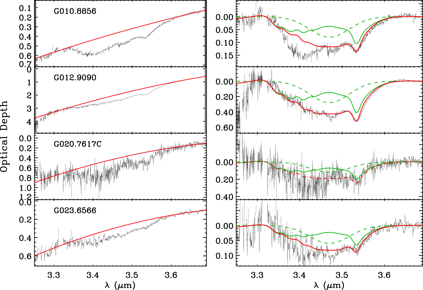
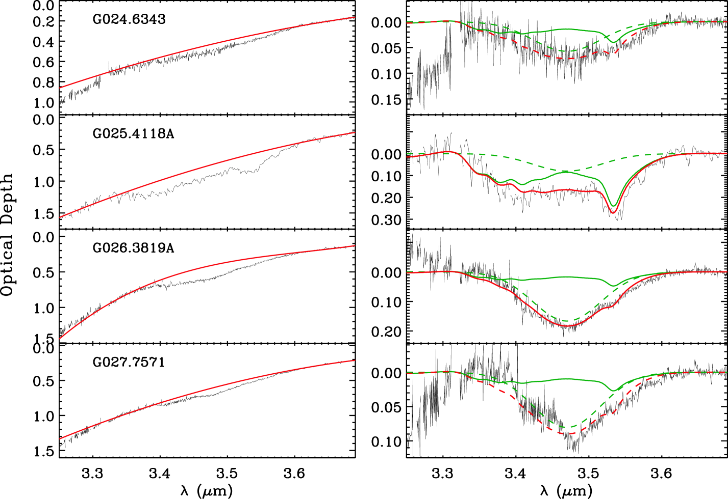
Figure 10: Portion of the $L-$band spectra of the MYSO sample. All targets show the 3.47 ${\rm\mu m}$ absorption band, likely caused by NH₃ hydrates, and some show signs of hydrocarbon absorption as well near 3.4 ${\rm\mu m}$ (e.g., G033.5237). The feature at 3.53 ${\rm\mu m}$ is attributed to CH₃OH ice. For each target, the left panel shows the adopted local polynomial baseline, and the right panel the baseline subtracted spectrum. In the right panels, the solid green line is a laboratory spectrum of CH₃OH ice at a temperature of 10 K (H₂O:CH₃OH:CO:NH₃=100:50:1:1; Hudgins et al. 1993) and the dashed green line a Gaussian. The sum of these fits is shown as a solid red line. For targets without a CH₃OH ice detection, a dashed red line is shown instead.

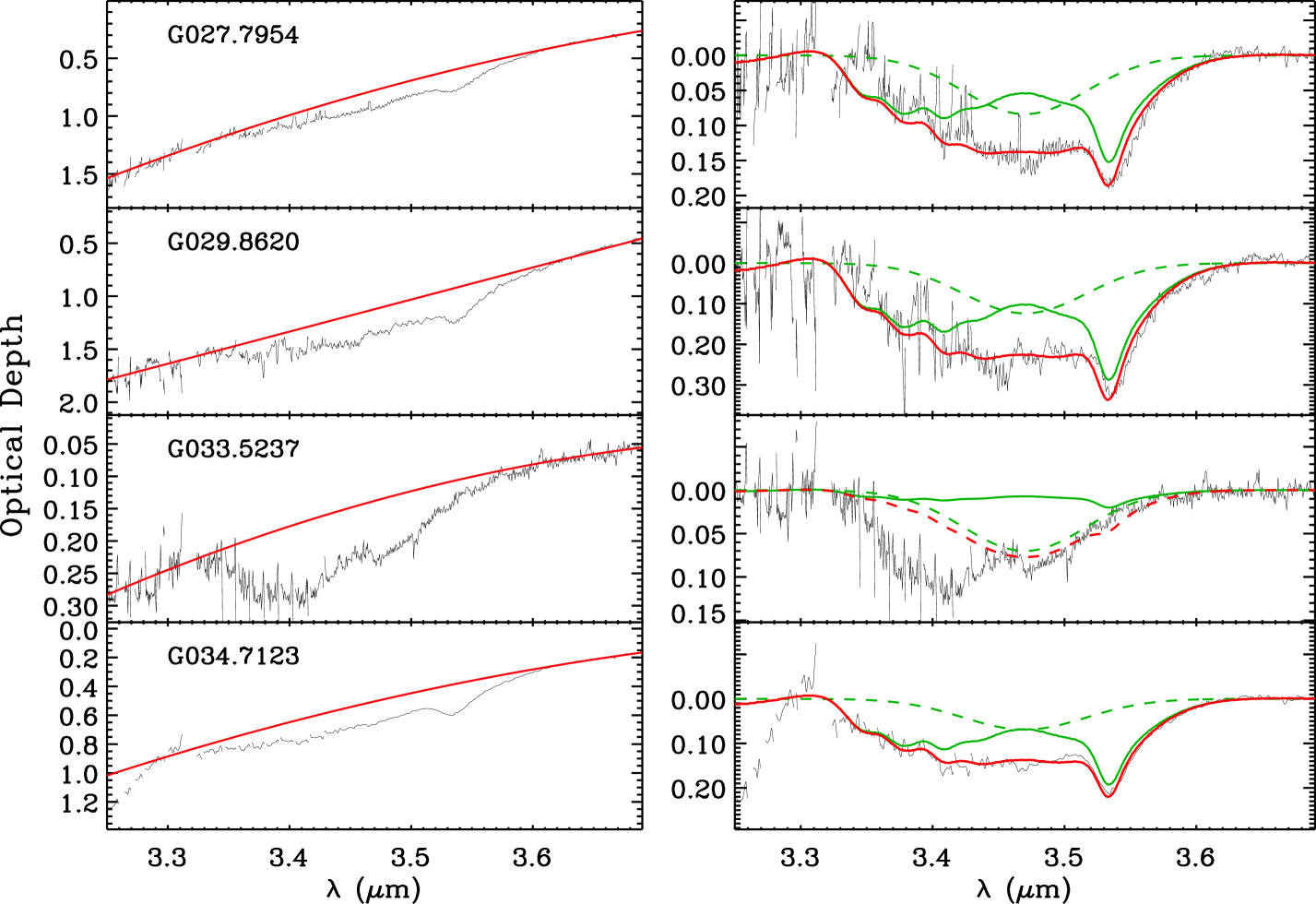
Figure 11: Extraction of the CH₃OH ice absorption band (solid green line) from the $L$-band spectra of the MYSO sample. For more details, see the caption of Figure 10.

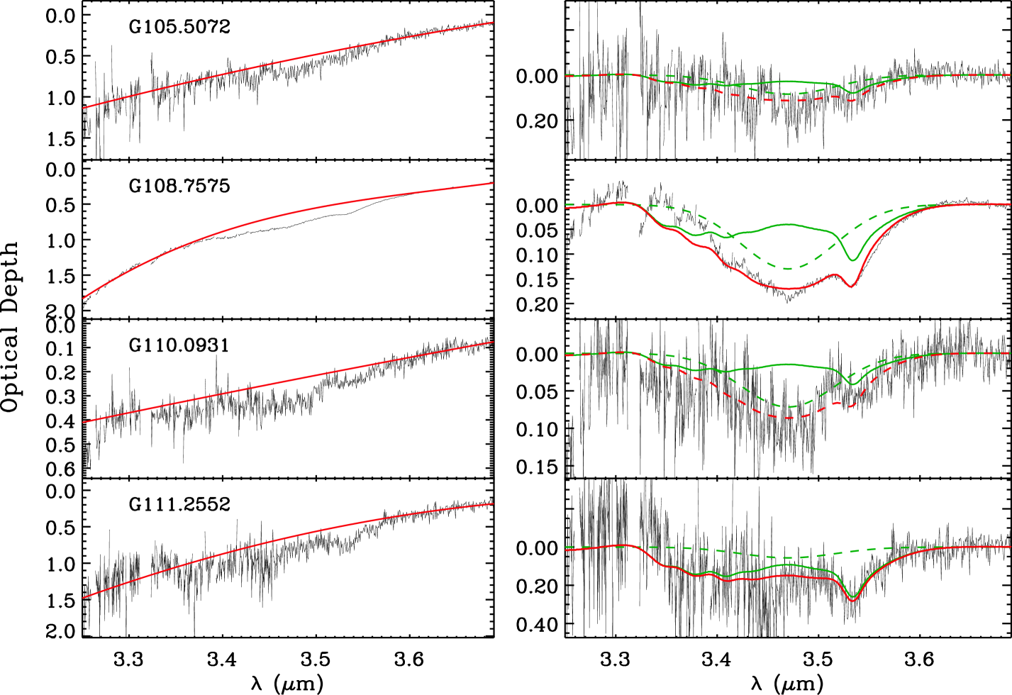
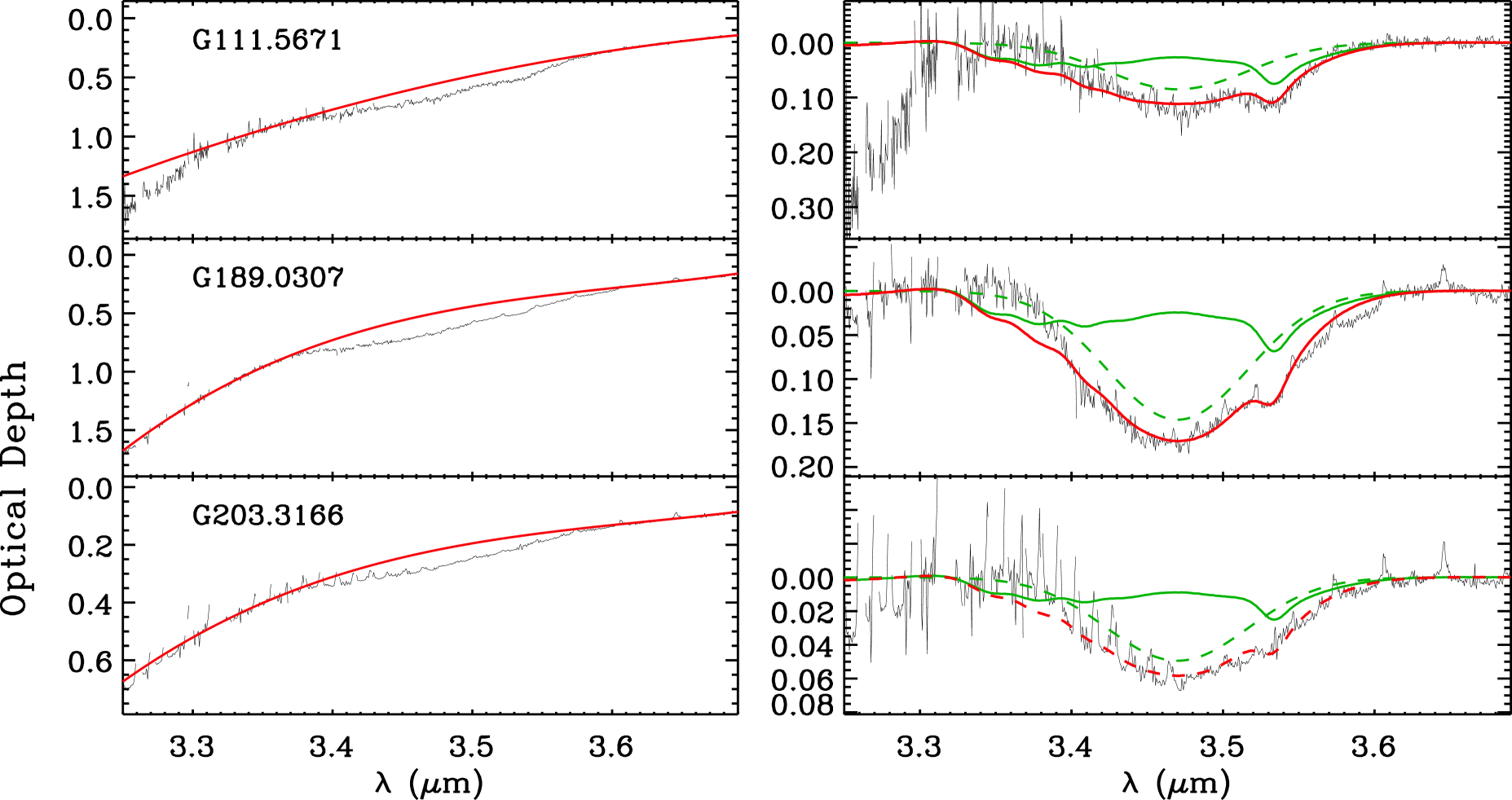
Figure 12: Extraction of the CH₃OH ice absorption band (solid green line) from the $L$-band spectra of the MYSO sample. For more details, see the caption of Figure 10.

4.3.5 H₂O

To be able to derive relative ice abundances, column densities for the most abundant ice species, H₂O, were derived as well. This was done as part of the continuum fitting process (§4.1). An integrated band strength of 2.0$\times 10^{-16}$ cm/molecule (Hagen et al., 1981) was used. The column densities reflect those of the small grains portion of the 3.0 ${\rm\mu m}$ band, excluding the long-wavelength wing, which may have a varied and uncertain origin. This approach was also adopted for low mass YSOs and background stars in previous work (e.g., Boogert et al. 2008). For a more in depth analysis of the profile of the 3.0 ${\rm\mu m}$ band of this and a larger sample of MYSOs, we refer to K. Emerson et al. (in preparation). The H₂O column densities are listed in Table 2.

4.4 OCS Laboratory Spectroscopy

The spectra of solid OCS in a range of astrophysically relevant ice mixtures and temperatures were measured by Hudgins et al. (1993), Palumbo et al. (1995), Ferrante et al. (2008), and Garozzo et al. (2010). Peak positions and FWHM values of the C-O stretch mode of OCS for non-irradiated mixtures are displayed in Figure 13a. The peak position depends strongly on the ice composition: mixtures with apolar species peak near 4.87-4.88 ${\rm\mu m}$, mixtures with H₂O peak at 4.88-4.89 ${\rm\mu m}$, and mixtures with CH₃OH near 4.90 ${\rm\mu m}$. The profiles of the apolar mixtures become much broader (factor of 2-3) upon heating, while the polar mixtures are very broad at temperatures of 10 K, and then dramatically narrow at higher temperatures.

The proton-irradiated ices studied in Ferrante et al. (2008), generally exhibit a different behavior (Figure 13b). This is confirmed by the proton-irradiation experiments of Garozzo et al. (2010). Upon heating, the peak position shifts to much longer wavelength (up to 4.915 ${\rm\mu m}$, the longest of all experiments), while its width does not change much, except for a narrowing for the H₂O:CO:SO₂ ice mixture. The strong shift must at least in part be related to the formation of new species in the ice, such as CO₃, CS₂, and CO₂, changing the dipole interactions.

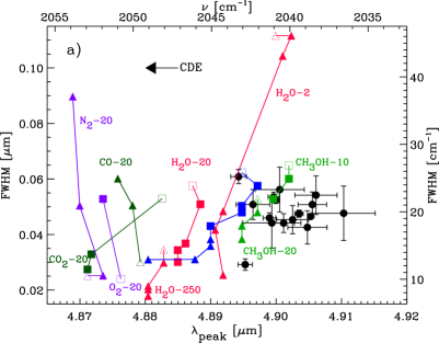
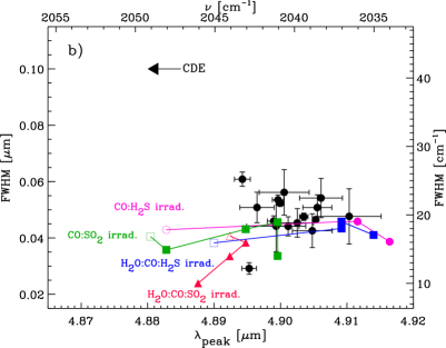
Figure 13: Panel (a): Peak position versus width for the profile of the C-O stretch mode of solid OCS as a function of mixing ratio and temperature for non-irradiated mixtures, taken from Hudgins et al. (1993), Palumbo et al. (1995), and Ferrante et al. (2008). Different ice mixtures are distinguished by different symbols and colors. Mixing ratios are labeled relative to OCS (e.g., ”CH₃OH-10” means a mixing ratio of CH₃OH:OCS=10:1). For a giving ice mixture, different temperatures are connected with a line. For each temperature series, the lowest temperature mixture is indicated with an open symbol. The unlabeled dark blue squares indicate a mixture of H₂O:CH₃OH:OCS=3:10:1, and the dark blue triangles of H₂O:CH₃OH:OCS=100:50:1. The peak position changes typically by the amount indicated by the black arrow if the OCS is present at concentrations $>10\%$ on grains with shapes of a Continuous Distribution of Ellipsoids (CDE), rather than on a flat surface as in the laboratory transmission spectra. The black bullets with error bars indicate the peak positions and widths observed toward the sample of MYSOs. Panel (b): Similar to panel (a), but here the observations (black bullets) are compared to the proton-irradiated mixtures of Ferrante et al. (2008).

Figure 13 also shows a comparison to the observations. Of the non-irradiated mixtures, ices rich in CH₃OH typically give the best match of peak position and FWHM. Of the mixtures without CH₃OH, only those with relatively high OCS/H₂O ($\sim$2) provide a match to some of the observed MYSOs, but this deteriorates when grain shape effects are taken into account, which typically shift the absorption band to shorter wavelengths. Grain shape effects are significant if OCS has a relatively high concentration ($\geq$10%). The best match in peak position and FWHM is in fact provided by the proton-irradiated CO:H₂S ices, as those are the only ones that cover the longest observed peak positions near 4.905 ${\rm\mu m}$. This might point to a relatively complex molecular environment for OCS.

4.5 Ice Correlations

To further constrain the molecular environment and formation history of OCS, its column density is plotted versus that of other species (Figure 14), and correlation coefficients are derived. A positive Spearman’s Rank coefficient ($\rho$) indicates the probability that there is a monotonically increasing relation, with a maximum of 1.0. This value is indicated in each panel, with the second number the significance of there being no correlation. The best correlations are found for OCS with the OCN^- and CH₃OH column densities ($\rho\sim$0.72), followed by CO_polar ($\rho\sim$0.65). The correlations are rather poor for OCS with the H₂O column ($\rho\sim$0.28) and there is no correlation with CO_apolar.

We investigated whether the rather poor correlation of OCS with H₂O could be an artifact related to underestimated H₂O column densities (and uncertainties) due to saturated 3.0 ${\rm\mu m}$ absorption bands. Inspection of Figures 1-3 shows that this could be the case for five MYSOs. But of those, G020.7617 was not included in the OCS version H₂O corelation due to the non-detection of OCS, G111.2552 was not included due to severe saturation of the 3.0 ${\rm\mu m}$ band, and G012.9090 is a well studied MYSO (W33A) for which $N$(H₂O) is quite reliable (e.g., Gibb et al. 2004). Excluding the remaining two targets (G105.5072 and G059.7831) from the correlation plot reduces the Spearman’s Rank coefficient from 0.28 to 0.21. Including those two targets, and artificially increasing their column density with a factor of 1.6 to force an improved correlation, improves the Spearman’s Rank coefficient somewhat (0.34), but it is still much poorer than the correlations of OCS with CH₃OH, OCN^-, and CO_polar.

The correlations among CH₃OH, OCN^-, and CO_polar are also investigated (Fig. 15). Indeed, as expected, the best correlation is that between CH₃OH and OCN^- ($\rho\sim$0.64). The correlations of CO_polar with CH₃OH ($\rho\sim$0.43) and with OCN^- ($\rho\sim$0.57) are poorer than that of OCS with CO_polar ($\rho\sim$0.65).

In summary, OCS, CH₃OH, and OCN^- correlate best with eachother, and somewhat poorer with CO_polar. There is no correlation of these species with H₂O and CO_apolar. Despite the reasonably good correlations found for OCS with the OCN^- and CH₃OH column densities, a linear model does not describe the observations well. The scatter in the datapoints is much larger than the uncertainties. At any given CH₃OH or OCN^- column density, the OCS column density varies by a factor of 2-3.

Figure 14: Correlation plots of the OCS column density versus that of other ice species towards MYSOs. The values in each top left corner are the Spearman’s Rank coefficient and each second number is the significance of there being no correlation.

Figure 15: Correlation plots of CH₃OH with OCN^- (panel (a)) and CO_polar (panel (b)), and of CO_polar with OCN^- (panel (c)). towards MYSOs. The values in each top left corner are the Spearman’s Rank coefficient and each second number is the significance of there being no correlation.

4.6 Abundance Distributions

The distribution of the ice abundances for the MYSOs and other target categories is shown in histograms (Figs. 16-18). The corresponding median abundances and upper and lower quartiles are listed in Table 5, following the format in (Öberg et al., 2011) and (Boogert et al., 2015). The distribution of the OCS ice abundances relative to CH₃OH is much narrower compared to abundances relative to H₂O ice (Fig. 16), consistent with the much better Spearman’s Rank coefficient (Fig. 14). It also shows the large improvement in sample size relative to previous work. No detections or significant upper limits of OCS ice abundances were made towards low mass YSOs and dense cloud background stars (Palumbo et al., 1997; Boogert et al., 2000; Gibb et al., 2004). Towards comets, OCS abundances relative to H₂O where published by Saki et al. (2020) and Figure 16 shows a distribution quite similar to that for MYSOs.

The abundance of CH₃OH relative to H₂O ice towards MYSOs appears to be fairly similar, or perhaps a little larger, compared to low mass YSOs and dense cloud background stars (Fig. 17). For OCN^- relative to H₂O ice, a fairly broad distribution is observed for MYSOs, with a peak at higher abundances compared to low mass YSOs. Towards dense cloud background stars, OCN^- has not yet been detected, with upper limits comparable to the detections towards low mass YSOs (Whittet et al., 2001b; Chu et al., 2020).

For CO ice, the abundances relative to H₂O ice are quite similar for MYSOs, low mass YSOs, and dense cloud background stars (Fig. 18). But while the abundances of the polar component of CO relative to H₂O ice are also quite similar across the different classes of objects, this is not the case for the apolar CO phase. Previous work on MYSOs (red hatched histograms in Fig. 18) showed a deficiency of the total CO and polar CO ices relative to low mass YSOs and background stars. In the current sample, this is no longer the case, their abundances are comparable. However, the deficiency of the apolar CO ice component in the current MYSO sample is consistent with previous work.

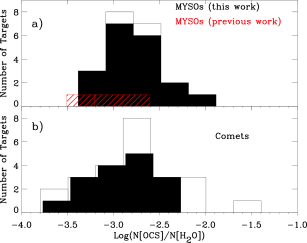
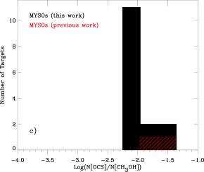
Figure 16: Distribution of the OCS ice abundance relative to H₂O ice towards MYSOs (panel (a)). The solid black histogram is for MYSO detections presented in this work. The unfilled histogram includes abundance upper limits. The hatched red histogram is for all OCS ice detections of previous work. Panel (b) shows the OCS abundance in comets (Saki et al., 2020), with the open histogram including upper limits. Panel (c) shows the OCS ice abundances relative to CH₃OH ice for the MYSOs presented in this (black) and previous (red) work.

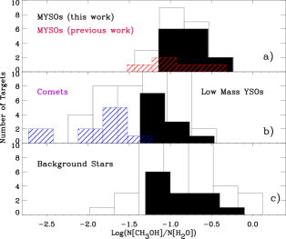
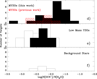
Figure 17: Panel (a): Distribution of the CH₃OH ice abundance relative to H₂O ice towards MYSOs. The solid black histogram is for MYSO detections presented in this work. The hatched red histogram is for all CH₃OH ice detections of previous work. Panel (b) shows the CH₃OH ice abundances toward low mass YSOs (black) and comets (blue hatched). Panel (c) shows CH₃OH ice abundances relative to H₂O ice for lines of sight tracing quiescent dense cloud material. In all panels the unfilled histogram includes abundance upper limits. Panels (d), (e), and (f) show the abundances of OCN^- ice relative to H₂O ice for MYSOs, low mass YSOs, and background stars, respectively.

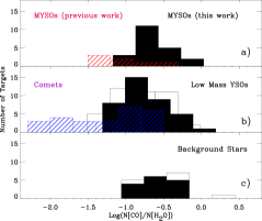
Figure 18: Panel (a): Distribution of the total CO ice abundance relative to H₂O ice towards MYSOs. The solid black histogram is for MYSO detections presented in this work. The hatched red histogram is for all CO ice detections of previous work. Panel (b) shows the CO ice abundances toward low mass YSOs (black) and comets (blue hatched). Panel (c) shows CO ice abundances relative to H₂O ice for lines of sight tracing quiescent dense cloud material. In all panels the unfilled histogram includes abundance upper limits. Panels (d), (e), and (f) show the abundances of CO ice in the polar phase relative to H₂O ice for MYSOs, low mass YSOs, and background stars, respectively. Panels (g), (h), and (i) show the abundances of CO ice in the apolar phase towards these same target categories.

Table 5: Median Ice Abundances 

Quantity	MYSOs	LYSOs	BG Stars	Comets
$N$(OCS)/$N$(H2O)$\times$100%	0.15${}_{0.12}^{0.28}$	$\cdots$	$\cdots$	0.14${}_{0.08}^{0.21}$
$N$(OCS)/$N$(CH3OH)$\times$100%	0.92${}_{0.74}^{1.42}$	$\cdots$	$\cdots$	$\cdots$
$N$(CH3OH)/$N$(H2O)$\times$100%	20${}_{8}^{26}$	5.6${}_{4.8}^{11.8}$	10${}_{7}^{21}$	1.7${}_{0.6}^{2.5}$
$N$(OCN-)/$N$(H2O)$\times$100%	1.53${}_{0.58}^{2.49}$	0.63${}_{0.39}^{0.77}$	$<0.2-0.9$	$\cdots$
$N$(COtotal)/$N$(H2O)$\times$100%	24${}_{15}^{31}$	15${}_{10}^{32}$	25${}_{12}^{43}$	7${}_{2}^{15}$
$N$(COpolar)/$N$(H2O)$\times$100%	14${}_{10}^{22}$	11${}_{8}^{17}$	13${}_{6}^{19}$	$\cdots$
$N$(COapolar)/$N$(H2O)$\times$100%	4.0${}_{2.5}^{10.8}$	11${}_{5}^{24}$	21${}_{12}^{35}$	$\cdots$

5 Discussion

The presented infrared spectroscopic survey of solid OCS towards 23 MYSOs provides observational constraints to the formation environment of sulfur-bearing species in interstellar and circumstellar ices. When compared with un-irradiated laboratory ice mixtures, the observed 4.90 ${\rm\mu m}$ C-O stretching mode band profiles of OCS are most consistent with CH₃OH-rich OCS ice mixtures, and do not favor H₂O, CO₂, and CO-rich environments. This confirms the early work by Palumbo et al. (1997) on a sample of three MYSOs. In our much larger sample, the identification of OCS in CH₃OH-rich mixtures is supported by a good correlation of the OCS and CH₃OH column densities, indeed much better than that with the H₂O and CO column densities.

Observations and models have shown that CH₃OH formation is strongly enhanced deep into dense clouds ($A_{\rm V}>9$, densities $\geq 10^{5}$ cm^-3), once much of the CO freezes out (Pontoppidan et al., 2004; Cuppen et al., 2009; Boogert et al., 2011; Chu et al., 2020). The good correlation of the OCS and CH₃OH column densities would then indicate that OCS is preferably formed in this later, dense stage of molecular clouds, or the envelopes of YSOs, where similar conditions occur. A direct accretion of OCS from the gas phase can be excluded, considering that gas phase OCS abundances are $\sim 1\times 10^{-5}$ relative to CO, orders of magnitude smaller than observed in the ices (Table 5). The route to solid state OCS might then be the oxidation of CS on the grains. At the same time, the oxidation of CO would likely produce CO₂, and indeed, the presence of CO₂ heavily diluted in CH₃OH ice is indicated by a long-wavelength shoulder on the 15 ${\rm\mu m}$ bending mode of solid CO₂ ice (Dartois et al., 1999; Gerakines et al., 1999). The abundance of this CO₂ relative to the CH₃OH column density varies between 5-30% (Pontoppidan et al., 2008), indicating that such oxidation reactions in the CO-rich ice phase are significant.

CS and CO are formed early in the cloud evolution, by gas phase ion-molecule reactions, when at low densities, C, S, and O are mostly in atomic form (e.g., Palumbo et al. 1997). Later gas phase chemistry does not modify CS, but converts S to SO. On the grain surfaces, early oxidation of CO and CS would make CO₂ and OCS and oxidation of S and SO makes SO₂. Evidently, at the same time, abundant H₂O ices are produced, and some CH₃OH formation is expected as well. Therefore, if OCS formation takes place early in the cloud’s lifetime, at relatively low densities ($\sim 10^{3}$ cm^-3), it is expected to be mixed with H₂O, CO₂, and CH₃OH. However, while the CO₂ abundance correlates very well with that of H₂O ice ($N$(CO₂)/$N$(H₂O)$\sim$ 20-30%, e.g., Gerakines et al. 1999), CH₃OH and OCS ice have not been detected at the level of $<1\%$ in these early ices. Our observations are consistent with the formation of the bulk of these species much deeper in the cloud.

A key question is if there is sufficient CS to produce the OCS abundance observed for the MYSO sample. In diffuse clouds and dense clouds, the gas phase CS/CO abundance ratio is $\sim 5\times 10^{-5}$ (Laas & Caselli 2019 and references therein). The observed median abundance of OCS ice relative to CO ice is two orders of magnitude larger at 6$\times 10^{-3}$ (Table 5). Much of the CO was converted to CH₃OH and CO₂, however. The ice abundances of CO, CH₃OH, and CO₂ are comparable (Table 5, Gerakines et al. 1999), resulting in a OCS/(CO+CH₃OH+CO₂) ice ratio of 2$\times 10^{-3}$. This is still a factor of $\sim 40$ larger than the CS/CO ratio produced by gas phase chemistry. In addition, much like CO ice is converted to H₂CO and CH₃OH, CS would be converted to H₂CS and CH₃SH as well (Lamberts, 2018). Observations toward a comet (Calmonte et al., 2016; Altwegg et al., 2019) and the envelopes of Class 0 protostar (Drozdovskaya et al., 2019) show $N$(CH₃SH)/$N$(CS)$\sim 1$. The order of magnitude enhancement of CS due to grain surface chemistry seen in the models of Laas & Caselli (2019), would not fully remedy this. Overall, CS appears to be only a minor precursor to OCS ice.

Sulfurization of CO ice is a more likely route to OCS. Laas & Caselli (2019) find that S atom addition reactions are dominant on the grains. Sulfur allotropes, such as suggested for the formation of abundant gas phase SO₂ in a hot core (Dungee et al., 2018), could also play a role. H₂S seems a reasonable candidate as well. The upper limits on the H₂S ice abundance ($<$0.3-1% relative to H₂O; Smith 1991) are larger than the OCS ice abundances and thus the observations currently do not constrain this possibility.

The production of OCS by energetic process may play a role as well. The peak positions and widths of the 4.90 ${\rm\mu m}$ band toward many of the observed targets are consistent with the proton-irradiated CO:H₂S=5:1 and CO:SO₂=5:1 ices, with or without H₂O, after a modest amount of heating to temperatures of $<$50 K (Fig. 13; Ferrante et al. 2008; see also Garozzo et al. 2010). Such irradiation would produce much CO₂, and minor amounts of C₃O₂, C₂O, HCO, CS₂, and for the SO₂-containing ices also O₃. Other than CO₂, which is also abundantly produced by grain surface chemistry, the latter species are not detected in the MYSO spectra, but not with significant upper limits. Indeed, in the irradiation experiments, the absorption strengths of the other species observed is much less than that of the 4.90 ${\rm\mu m}$ OCS band. A deep search with JWST is needed to further constrain the irradiation history of the interstellar ices.

The starting mixture in these irradiation experiments is CO:H₂S=5:1 and CO:SO₂=5:1. The presence of H₂S in CO-rich ices locates the ices at lower densities, where H₂S would be formed via hydrogenation reactions on the grain surface, while the good correlation of OCS with CH₃OH indicates the formation during a high density phase. SO₂, on the other hand, was suggested to be present in a CH₃OH-rich environment, following a tentative detection by Boogert et al. (1997). At an SO₂ abundance of 0.3% relative to H₂O towards the MYSO W33A (G012.9090-00.2607), the abundance relative to CO ice is 3.5%. This is within an order of magnitude of the composition of the initial laboratory ice, and thus irradiation of SO₂-containing ices could be the source of the observed OCS ices. A more quantitative assessment is beyond the scope of this work, and would also benefit from SO₂ ice measurements in a wider variety of sight-lines. Also, other S-bearing species in the CO-rich ice, such as CS and S allotropes may produce OCS in the irradiation process as well. Indeed, free S atoms readily react with CO to form OCS (Ferrante et al., 2008).

Finally, we note that despite the correlation of OCS column densities with the species mentioned above, the scatter in the correlations is of the order of a factor of 2. This implies that the OCS production is quite strongly dependent on specific local conditions (radiation fields, ice temperatures). This is reminiscent of conclusions that were drawn for the production of OCN^- (van Broekhuizen et al., 2005).

5.1 OCN^-

The correlation of OCS with OCN^- is as good as that with CH₃OH (Fig. 14), and indeed OCN^- and CH₃OH also correlate well with eachother (Fig. 15). In a study of low mass YSOs, van Broekhuizen et al. (2005) found that OCN^- is present in both CO-rich and polar environments, claiming that OCN^- is formed in a CO-rich environment (short-wavelength component) and survives in a polar-CO environment (long-wavelength component; see also Öberg et al. 2011). This is confirmed by a correlation of the short-wavelength component with CO in an apolar environment, and of the long-wavelength component with polar CO ices. For our MYSO sample, the short wavelength component is detected in just a few cases. The long-wavelength component indeed correlates much better with the polar than with the apolar ices. Thus, overall the idea of OCN^- being produced in a CO-rich environment is confirmed. For our MYSO sample, much of the CO has already been converted to other species.

While it was shown that OCN^- is easily produced at low temperatures by acid base chemistry of HNCO and NH₃ mixtures (Raunier et al., 2004), the apolar ices are expected to be NH₃-poor, just like they are H₂O-poor. Perhaps another base enables this reaction. On the other hand, it was shown that the presence of N in CO-rich ices leads (non-energetically) to the formation of both HNCO and NH₃ (Fedoseev et al., 2015) as a result of hydrogen addition and abstraction reactions.

5.2 Comparing YSOs, Dense Clouds, and Cometary Ices

In a statistical comparison of YSO and cometary ice abundances, Öberg et al. (2011) concluded that comets are carbon and nitrogen-poor. This could hint to the effects of ice processing in protoplanetary disks, or that compared to the distribution of ice abundances of low mass YSOs, the early Sun resembled the YSOs with low C and N ice abundances. One possible cause of low C and N abundances could be the presence of nearby massive stars, that sublimate or photodesorb the most volatile (CO, N₂) ices. The Sun was indeed most likely formed in a cluster (Adams, 2010).

Re-assessing the comparison between YSOs and comets, using the vastly increased MYSO sample, we find that, in contrast to the lower abundances in previous work, MYSOs have CO ice abundances that are comparable to those of low mass YSOs and background stars (Fig. 18a-c). About 50% of the comets have CO ice abundances below those of MYSOs and low mass YSOs. The large heterogeneity of the cometary CO ice abundances is also apparent, probably reflecting their processing history. Comets are also particularly poor in CH₃OH ices (Fig. 17)), especially when compared to the new sample of MYSOs.

In contrast to carbon-bearing molecules, comets do not show a deficiency in the OCS abundance (Fig. 16)). This is surprising, considering that we find that OCS is mixed with CH₃OH-rich ices. This could point to the additional production of OCS in the protoplantary disk phase. Studies of OCS in low mass YSOs will be enabled by JWST. A tentative detection by the AKARI space telescope towards the edge-on disk IRC L1041-2 indicates a very high OCS ice abundance of 1.1% relative to H₂O (Aikawa et al., 2012), which is 50% more than the MYSO with the largest OCS abundance (G010.8856+00.1221; Table 4)

As for the comparison between MYSOs, low mass YSOs and dense cloud background stars, MYSOs are CH₃OH and OCN^--rich. The total and polar CO ice abundances are quite similar, but MYSOs do appear to have significantly less apolar ices. This is consistent with a more efficient conversion of CO to CH₃OH and OCN^- in the ices. One should keep in mind, however, that the low mass YSO and dense cloud background star samples are presently relatively small.

6 Conclusions and Future Work

Infrared 2-5 ${\rm\mu m}$ spectra of a sample of twenty-three deeply embedded MYSOs were studied with the primary goal to study the abundance of solid state OCS via the C-O stretch mode at 4.90 ${\rm\mu m}$. The following conclusions are drawn:

1. The OCS band at 4.90 ${\rm\mu m}$ was detected in twenty MYSO lines of sight, increasing the sample by more than a factor of 5.

2. The absorption profile of the OCS band shows little variation from source to source and is consistent with mixtures of OCS embedded in CH₃OH-rich ices, or mildly heated proton-irradiated CO:H₂S ices.

3. All twenty-three MYSOs show CO and H₂O ice absorption, and most show absorption by OCN^- and CH₃OH.

4. The OCS column density correlates well with that of CH₃OH and OCN^-, and polar CO ice, but not with H₂O and apolar CO ice. This firmly establishes that OCS ice is formed together with CH₃OH and OCN^-, deep inside dense clouds or protostellar envelopes.

5. The median ice abundance towards the MYSO sample, as a percentage of H₂O ice is CO:CH₃OH:OCN^-:OCS=24:20:1.53:0.15

6. It is deduced that CS is not the main precursor to OCS, because its abundance is too low by at least a factor of $\sim$40. Sulfurization of CO is likely needed. The source of this sulfur is unclear. Perhaps sulfur atoms or allotropes. The H₂S ice abundance is insufficiently constrained.

7. The OCS abundances relative to H₂O ice towards MYSOs and comets are remarkably similar. This contrasts with CH₃OH, which shows a deficit for comets. Perhaps additional OCS is formed in protoplanetary disk environments.

8. Compared to low mass YSOs, MYSOs show an excess of OCN^- ice in a significant fraction of the targets. The CO and CH₃OH ice abundances are comparable to those observed towards low mass YSOs and dense cloud background stars. It should be noted that the low mass YSO and background star samples are fairly small, but this will be improved upon with JWST observations in the near future. Evidently, the current lack of detections of OCS ice towards low mass YSOs and background stars needs to be improved upon to form the trail of sulfur to comets. Indeed, the presented IRTF/SpeX 2-5 ${\rm\mu m}$ spectra of this sample of MYSO, most of which would saturate the JWST/NIRSpec and NIRCam WFSS detectors, will serve as a reference for the future JWST observations.

References

- Adams (2010) Adams, F. C. 2010, ARA&A, 48, 47, doi: 10.1146/annurev-astro-081309-130830
- Aikawa et al. (2012) Aikawa, Y., Kamuro, D., Sakon, I., et al. 2012, A&A, 538, A57, doi: 10.1051/0004-6361/201015999
- Altwegg et al. (2019) Altwegg, K., Balsiger, H., & Fuselier, S. A. 2019, ARA&A, 57, 113, doi: 10.1146/annurev-astro-091918-104409
- Altwegg et al. (2020) Altwegg, K., Balsiger, H., Hänni, N., et al. 2020, Nature Astronomy, 4, 533, doi: 10.1038/s41550-019-0991-9
- Boogert et al. (2002) Boogert, A. C. A., Blake, G. A., & Tielens, A. G. G. M. 2002, ApJ, 577, 271, doi: 10.1086/342176
- Boogert et al. (2015) Boogert, A. C. A., Gerakines, P. A., & Whittet, D. C. B. 2015, ARA&A, 53, 541, doi: 10.1146/annurev-astro-082214-122348
- Boogert et al. (1997) Boogert, A. C. A., Schutte, W. A., Helmich, F. P., Tielens, A. G. G. M., & Wooden, D. H. 1997, A&A, 317, 929
- Boogert et al. (2000) Boogert, A. C. A., Tielens, A. G. G. M., Ceccarelli, C., et al. 2000, A&A, 360, 683. https://arxiv.org/abs/astro-ph/0005030
- Boogert et al. (2008) Boogert, A. C. A., Pontoppidan, K. M., Knez, C., et al. 2008, ApJ, 678, 985, doi: 10.1086/533425
- Boogert et al. (2011) Boogert, A. C. A., Huard, T. L., Cook, A. M., et al. 2011, ApJ, 729, 92, doi: 10.1088/0004-637X/729/2/92
- Brooke et al. (1999) Brooke, T. Y., Sellgren, K., & Geballe, T. R. 1999, ApJ, 517, 883, doi: 10.1086/307237
- Calmonte et al. (2016) Calmonte, U., Altwegg, K., Balsiger, H., et al. 2016, MNRAS, 462, S253, doi: 10.1093/mnras/stw2601
- Charnley et al. (1992) Charnley, S. B., Tielens, A. G. G. M., & Millar, T. J. 1992, ApJ, 399, L71, doi: 10.1086/186609
- Chiar et al. (1995) Chiar, J. E., Adamson, A. J., Kerr, T. H., & Whittet, D. C. B. 1995, ApJ, 455, 234, doi: 10.1086/176571
- Chiar et al. (2011) Chiar, J. E., Pendleton, Y. J., Allamandola, L. J., et al. 2011, ApJ, 731, 9, doi: 10.1088/0004-637X/731/1/9
- Chu et al. (2020) Chu, L. E. U., Hodapp, K., & Boogert, A. 2020, ApJ, 904, 86, doi: 10.3847/1538-4357/abbfa5
- Cuppen et al. (2009) Cuppen, H. M., van Dishoeck, E. F., Herbst, E., & Tielens, A. G. G. M. 2009, A&A, 508, 275, doi: 10.1051/0004-6361/200913119
- Cushing et al. (2004) Cushing, M. C., Vacca, W. D., & Rayner, J. T. 2004, PASP, 116, 362, doi: 10.1086/382907
- Dartois et al. (1999) Dartois, E., Demyk, K., d’Hendecourt, L., & Ehrenfreund, P. 1999, A&A, 351, 1066
- Dartois & d’Hendecourt (2001) Dartois, E., & d’Hendecourt, L. 2001, A&A, 365, 144, doi: 10.1051/0004-6361:20000174
- Disanti & Mumma (2008) Disanti, M. A., & Mumma, M. J. 2008, Space Sci. Rev., 138, 127, doi: 10.1007/s11214-008-9361-0
- Drozdovskaya et al. (2019) Drozdovskaya, M. N., van Dishoeck, E. F., Rubin, M., Jørgensen, J. K., & Altwegg, K. 2019, MNRAS, 490, 50, doi: 10.1093/mnras/stz2430
- Dungee et al. (2018) Dungee, R., Boogert, A., DeWitt, C. N., et al. 2018, ApJ, 868, L10, doi: 10.3847/2041-8213/aaeda9
- Fedoseev et al. (2015) Fedoseev, G., Ioppolo, S., Zhao, D., Lamberts, T., & Linnartz, H. 2015, MNRAS, 446, 439, doi: 10.1093/mnras/stu2028
- Ferrante et al. (2008) Ferrante, R. F., Moore, M. H., Spiliotis, M. M., & Hudson, R. L. 2008, ApJ, 684, 1210, doi: 10.1086/590362
- Garozzo et al. (2010) Garozzo, M., Fulvio, D., Kanuchova, Z., Palumbo, M. E., & Strazzulla, G. 2010, A&A, 509, A67, doi: 10.1051/0004-6361/200913040
- Gerakines et al. (1999) Gerakines, P. A., Whittet, D. C. B., Ehrenfreund, P., et al. 1999, ApJ, 522, 357, doi: 10.1086/307611
- Gibb et al. (2004) Gibb, E. L., Whittet, D. C. B., Boogert, A. C. A., & Tielens, A. G. G. M. 2004, ApJS, 151, 35, doi: 10.1086/381182
- Goto et al. (2021) Goto, M., Vasyunin, A. I., Giuliano, B. M., et al. 2021, A&A, 651, A53, doi: 10.1051/0004-6361/201936385
- Grim et al. (1991) Grim, R. J. A., Baas, F., Geballe, T. R., Greenberg, J. M., & Schutte, W. A. 1991, A&A, 243, 473
- Hagen et al. (1981) Hagen, W., Tielens, A. G. G. M., & Greenberg, J. M. 1981, Chemical Physics, 56, 367, doi: 10.1016/0301-0104(81)80158-9
- Herbst & van Dishoeck (2009) Herbst, E., & van Dishoeck, E. F. 2009, ARA&A, 47, 427, doi: 10.1146/annurev-astro-082708-101654
- Hudgins et al. (1993) Hudgins, D. M., Sandford, S. A., Allamandola, L. J., & Tielens, A. G. G. M. 1993, ApJS, 86, 713, doi: 10.1086/191796
- Indebetouw et al. (2005) Indebetouw, R., Mathis, J. S., Babler, B. L., et al. 2005, ApJ, 619, 931, doi: 10.1086/426679
- Ioppolo et al. (2011) Ioppolo, S., van Boheemen, Y., Cuppen, H. M., van Dishoeck, E. F., & Linnartz, H. 2011, MNRAS, 413, 2281, doi: 10.1111/j.1365-2966.2011.18306.x
- Jiang et al. (1975) Jiang, G. J., Person, W. B., & Brown, K. G. 1975, J. Chem. Phys., 62, 1201, doi: 10.1063/1.430634
- Kerkhof et al. (1999) Kerkhof, O., Schutte, W. A., & Ehrenfreund, P. 1999, A&A, 346, 990
- Laas & Caselli (2019) Laas, J. C., & Caselli, P. 2019, A&A, 624, A108, doi: 10.1051/0004-6361/201834446
- Lamberts (2018) Lamberts, T. 2018, A&A, 615, L2, doi: 10.1051/0004-6361/201832830
- Levison et al. (2010) Levison, H. F., Duncan, M. J., Brasser, R., & Kaufmann, D. E. 2010, Science, 329, 187, doi: 10.1126/science.1187535
- Lumsden et al. (2013) Lumsden, S. L., Hoare, M. G., Urquhart, J. S., et al. 2013, ApJS, 208, 11, doi: 10.1088/0067-0049/208/1/11
- Mumma & Charnley (2011) Mumma, M. J., & Charnley, S. B. 2011, ARA&A, 49, 471, doi: 10.1146/annurev-astro-081309-130811
- Öberg et al. (2011) Öberg, K. I., Boogert, A. C. A., Pontoppidan, K. M., et al. 2011, ApJ, 740, 109, doi: 10.1088/0004-637X/740/2/109
- Palumbo et al. (1997) Palumbo, M. E., Geballe, T. R., & Tielens, A. G. G. M. 1997, ApJ, 479, 839, doi: 10.1086/303905
- Palumbo et al. (1995) Palumbo, M. E., Tielens, A. G. G. M., & Tokunaga, A. T. 1995, ApJ, 449, 674, doi: 10.1086/176088
- Pomohaci et al. (2017) Pomohaci, R., Oudmaijer, R. D., Lumsden, S. L., Hoare, M. G., & Mendigutía, I. 2017, MNRAS, 472, 3624, doi: 10.1093/mnras/stx2196
- Pontoppidan et al. (2014) Pontoppidan, K. M., Salyk, C., Bergin, E. A., et al. 2014, in Protostars and Planets VI, ed. H. Beuther, R. S. Klessen, C. P. Dullemond, & T. Henning, 363
- Pontoppidan et al. (2004) Pontoppidan, K. M., van Dishoeck, E. F., & Dartois, E. 2004, A&A, 426, 925, doi: 10.1051/0004-6361:20041276
- Pontoppidan et al. (2003) Pontoppidan, K. M., Fraser, H. J., Dartois, E., et al. 2003, A&A, 408, 981, doi: 10.1051/0004-6361:20031030
- Pontoppidan et al. (2008) Pontoppidan, K. M., Boogert, A. C. A., Fraser, H. J., et al. 2008, ApJ, 678, 1005, doi: 10.1086/533431
- Raunier et al. (2004) Raunier, S., Chiavassa, T., Marinelli, F., & Aycard, J.-P. 2004, Chemical Physics, 302, 259, doi: 10.1016/j.chemphys.2004.04.013
- Rayner et al. (2003) Rayner, J. T., Toomey, D. W., Onaka, P. M., et al. 2003, PASP, 115, 362, doi: 10.1086/367745
- Saki et al. (2020) Saki, M., Gibb, E. L., Bonev, B. P., et al. 2020, AJ, 160, 184, doi: 10.3847/1538-3881/aba522
- Smith (1991) Smith, R. G. 1991, MNRAS, 249, 172, doi: 10.1093/mnras/249.1.172
- Terada & Tokunaga (2012) Terada, H., & Tokunaga, A. T. 2012, ApJ, 753, 19, doi: 10.1088/0004-637X/753/1/19
- Tielens & Hagen (1982) Tielens, A. G. G. M., & Hagen, W. 1982, A&A, 114, 245
- Tielens et al. (1991) Tielens, A. G. G. M., Tokunaga, A. T., Geballe, T. R., & Baas, F. 1991, ApJ, 381, 181, doi: 10.1086/170640
- Vacca et al. (2003) Vacca, W. D., Cushing, M. C., & Rayner, J. T. 2003, PASP, 115, 389, doi: 10.1086/346193
- van Broekhuizen et al. (2004) van Broekhuizen, F. A., Keane, J. V., & Schutte, W. A. 2004, A&A, 415, 425, doi: 10.1051/0004-6361:20034161
- van Broekhuizen et al. (2005) van Broekhuizen, F. A., Pontoppidan, K. M., Fraser, H. J., & van Dishoeck, E. F. 2005, A&A, 441, 249, doi: 10.1051/0004-6361:20041711
- Visser et al. (2009) Visser, R., van Dishoeck, E. F., Doty, S. D., & Dullemond, C. P. 2009, A&A, 495, 881, doi: 10.1051/0004-6361/200810846
- Watanabe & Kouchi (2002) Watanabe, N., & Kouchi, A. 2002, ApJ, 571, L173, doi: 10.1086/341412
- Whittet et al. (2001a) Whittet, D. C. B., Gerakines, P. A., Hough, J. H., & Shenoy, S. S. 2001a, ApJ, 547, 872, doi: 10.1086/318421
- Whittet et al. (2001b) Whittet, D. C. B., Pendleton, Y. J., Gibb, E. L., et al. 2001b, ApJ, 550, 793, doi: 10.1086/319794
- Whittet et al. (1998) Whittet, D. C. B., Gerakines, P. A., Tielens, A. G. G. M., et al. 1998, ApJ, 498, L159, doi: 10.1086/311318