An Efficient Nonlinear Acceleration method that Exploits Symmetry of the Hessian
Abstract
Nonlinear acceleration methods are powerful techniques to speed up fixed-point iterations. However, many acceleration methods require storing a large number of previous iterates and this can become impractical if computational resources are limited. In this paper, we propose a nonlinear Truncated Generalized Conjugate Residual method (nlTGCR) whose goal is to exploit the symmetry of the Hessian to reduce memory usage. The proposed method can be interpreted as either an inexact Newton or a quasi-Newton method. We show that, with the help of global strategies like residual check techniques, nlTGCR can converge globally for general nonlinear problems and that under mild conditions, nlTGCR is able to achieve superlinear convergence. We further analyze the convergence of nlTGCR in a stochastic setting. Numerical results demonstrate the superiority of nlTGCR when compared with several other competitive baseline approaches on a few problems. Our code will be available in the future.
1 Introduction
In this paper, we consider solving the fixed-point problem:
| (1) |
This problem has received a surge of interest due to its wide range of applications in mathematics, computational science and engineering. Most optimization algorithms are iterative, and their goal is to find a related fixed-point of the form (1), where is the iteration mapping which can potentially be nonsmooth or noncontractive. When the optimization problem is convex, is typically nonexpansive, and the solution set of the fixed-point problem is the same as that of the original optimization problem, or closely related to it. Consider the simple fixed-point iteration which produces a sequence of iterates . When the iteration converges, its limit is a fixed-point, i.e., . However, an issue with fixed-point iteration is that it does not always converge, and when it does, it might reach the limit very slowly.
To address this issue, a number of acceleration methods have been proposed and studied over the years, such as the reduced-rank extrapolation (RRE) [58], minimal-polynomial extrapolation (MPE) [12], modified MPE (MMPE) [33], and the vector -algorithms [8]. Besides these algorithms, Anderson Acceleration (AA) [1] has received enormous recent attention due to its nice properties and its success in machine learnin applications [56, 22, 57, 14, 60, 44, 25, 63]. In practice, since computing the Hessian of the objective function is commonly difficult or even unavailable, AA can be seen as a practical alternative to Newton’s method [34]. Also, compared with the classical iterative methods such as the nonlinear conjugate gradient (CG) method [24], no line-search or trust-region technique is performed in AA, and this is a big advantage in large-scale unconstrained optimization. Empirically, it is observed that AA is quite successful in accelerating convergence. We refer readers to [9] for a recent survey of acceleration methods.
However, classical AA has one undesirable disadvantage in that it is expensive in terms of memory as well as computational cost, especially in a nonconvex stochastic setting, where only sublinear convergence can be expected when only stochastic gradients can be accessed [3]. In light of this, a number of variants of AA have been proposed which aim at improving its performance and robustness (e.g., [39, 63, 62, 56, 67]). The above-cited works focus on improving the convergence behavior of AA, but they do not consider reducing the memory cost. In machine learning, we often encounter practical situations where the number of parameters is quite large and for this reason, it is not practical to use a large number of vectors in the acceleration methods. It is not clear whether or not the symmetric structure of the Hessian can be exploited in a scheme like AA to reduce the memory cost while still maintaining the convergence guarantees. In this paper, we will demonstrate how this can be accomplished with a new algorithm that is superior to AA in practice.
Our contributions. This paper develops a nonlinear acceleration method, nonlinear Truncated Generalized Conjugate Residual method (nlTGCR), that takes advantage of symmetry. This work is motivated by the observation that the Hessian of a nonlinear function, or the Jacobian of a gradient of a mapping, is symmetric and therefore more effective, conjugate gradient-like schemes can be exploited.
We demonstrate that nonlinear acceleration methods can benefit from the symmetry property of the Hessian. In particular, we study both linear and nonlinear problems and give a systematic analysis of TGCR and nlTGCR. We show that TGCR is efficient and optimal for linear problems. By viewing the method from the angle of an inexact Newton approach, we also show that adding a few global convergence strategies ensures that nlTGCR can achieve global convergence guarantees.
We complement our theoretical results with numerical simulations on several different problems. The experimental results demonstrate advantages of our methods. To the best of our knowledge, this is still the first work to investigate and improve the AA dynamics by exploiting symmetry of the Hessian.
Related work. Designing efficient optimization methods has received much attention. Several recent works [65, 4, 40, 48, 18] consider second order optimization methods that employ sketching or approximation techniques. Different from these approaches, our method is a first-order method that utilizes symmetry of the Hessian instead of constructing it. A variant of inexact Newton method was proposed in [47] where the least-squares sub-problems are solved approximately using Minimum Residual method. Similarly, a new type of quasi Newton symmetric update [54] uses several secant equations in a least-squares sense. These approaches have the same goal as ours. However, they are more closely related to a secant or a multi-secant technique, and as will be argued it does a better job of capturing the nonlinearity of the problem. [63] proposed a short-term AA algorithm that is different from ours because it is still based on the parameter sequence instead of the gradient sequence and does not exploit symmetry of the Hessian.
2 Background
2.1 Extrapolation, acceleration, and the Anderson Acceleration procedure
Consider a general fixed-point problem and the associated fixed-point iteration as shown in (1). Denote by the residual vector at the th iteration. Classical extrapolation methods including RRE, MPE and the vector -Algorithm, have been designed to accelerate the convergence of the original sequence by generating a new and independent sequence of the form: . An important characteristic of these classical extrapolation methods is that the two sequences are not mixed in the sense that no accelerated item , is used to produce the iterate . These extrapolation methods must be distinguished from acceleration methods such as the AA procedure which aim at generating their own sequences to find a fixed point of a certain mapping .
AA was originally designed to solve a system of nonlinear equations written in the form [1, 61, 41, 30]. Denote . AA starts with an initial and sets , where is a parameter. At step we define and along with the differences:
| (2) | ||||
We then define the next AA iterate as follows:
| (3) | ||||
| (4) |
To define the next iterate in (3) the algorithm uses the term where is the current accelerated iterate. AA belongs to the class of multi-secant methods. Indeed, the approximation (3) can be written as:
| (5) |
Thus, can be seen as an update to the (approximate) inverse Jacobian
| (6) |
and is the minimizer of under the multi-secant condition of type II 111Type I Broyden conditions involve approximations to the Jacobian, while type II conditions deal with the inverse Jacobian.
| (7) |
This link between AA and Broyden multi-secant type updates was first unraveled by Eyert [21] and expanded upon in [46].
2.2 Inexact and quasi-Newton methods
Given a nonlinear system of equations . Inexact Newton methods [15, 10], start with an initial guess and compute a sequence of iterates as follows
| Solve | (8) | |||||
| Set | (9) |
Here, is the Jacobian of at the current iterate . In (8) the system is solved inexactly, typically by some iterative method. In quasi-Newton methods [17, 17, 54], the inverse of the Jacobian is approximated progressively. Because it is the inverse Jacobian that is approximated, the method is akin to Broyden’s second (or type-II) update method. This method replaces Newtons’s iteration: with where approximates the inverse of the Jacobian at by the update formula in which is defined in different ways see [46] for details.
3 Exploiting symmetry
In the following, we specifically consider the case where the nonlinear mapping is the gradient of some objective function to be minimized, i.e.,
In this situation, the Jacobian of becomes the Hessian of . An obvious observation here is that the symmetry of the Hessian is not taken into account in the approximate inverse Hessian update formula (6). This has only been considered in the literature (very) recently (e.g., [6, 55, 7]). In a 1983 report, [53] showed that the matrix obtained by a multi-secant method that satisfies the secant condition (7) is symmetric iff the matrix is symmetric. It is possible to explicitly force symmetry by employing generalizations of the symmetric versions of Broyden-type methods. Thus, the authors of [6, 7] developed a multisecant version of the Powell Symmetric Broyden (PSB) update due to Powell [45] while the article [55] proposed a symmetric multisecant method based on the popular Broyden-Fletcher-Goldfarb-Shanno (BFGS) approach as well as the Davidon-Fletcher-Powell (DFP) update. However, there are a number of issues with the symmetric versions of multisecant updates, some of which are discussed in [55].
We observe that when we are close to the limit, the condition is nearly satisfied. This is because if is the limit with we can write
| (10) | ||||
This translates to from which it follows that which is a symmetric matrix under mild smoothness conditions on . Therefore, the issue of symmetry can be mitigated if we are able to develop nonlinear acceleration methods that take advantage of near-symmetry.
3.1 The linear case: Truncated GCR (TGCR)
We first consider solving the linear system with a general matrix . The Generalized Conjugate Residual (GCR) algorithm, see, e.g., [19, 51], solves this linear system by building a sequence of search directions , for at step so that the vectors are orthogonal to each other. With this property it is easy to generate iterates that minimize the residual at each step, and this leads to GCR, see [51, pp 195-196] for details.
Next we will make two changes to GCR. First, we will develop a truncated version in which any given is orthogonal to the previous ’s only. This is dictated by practical considerations, because keeping all vectors may otherwise require too much memory. Second, we will keep a set of vectors for the ’s and another set for the vectors , for at step in order to avoid unnecessary additional products of the matrix with vectors. The Truncated GCR (TGCR) is summarized in Algorithm 1.
With we obtain the non-restarted GCR method, which is equivalent to the non-restarted (i.e., full) GMRES. However, when is symmetric, but not necessarily symmetric positive definite, then TGCR (1) is identical with TGCR (m) in exact arithmetic. This leads to big savings both in terms of memory and in computational costs.
Theorem 3.1.
When the coefficient matrix is symmetric, TGCR (m) generates the same iterates as TGCR (1) for any . In addition, when is positive definite, the -th residual vector satisfies the following inequality where is the spectral condition number of :
| (11) |
3.2 The nonlinear case: nlTGCR
Assume now that we want to solve the nonlinear problem We need to make three major changes to Algorithm 1. First, any residual is now the negative of so Line 2 and Line 7 must be replaced by and , respectively. In addition, we originally need to calculate the products and in Line 2 and Line 8 respectively. Here needs to be replaced by the Jacobian of at the current iterate. We also use the notation , and . The most important change is in lines 5-6 where of Algorithm 1 needs to be replaced by a vector . This is because when we write the linear model used in the form of an inexact Newton method:
| (12) | ||||
The projection method that minimizes the norm of the right-hand side determines in such a way that
| (13) | ||||
where it is assumed the ’s are fully orthogonal. Note that in the linear case, it can be shown that has only one nonzero component when one assumes that the vectors are fully orthogonal, i.e., that always. The nonlinear version of TGCR (m) is summarized in Algorithm 2 where the indication ‘Use Frechet’ means that the vector is to be computed as for some small .
Remark.
nlTGCR (m) requires 2 function evaluations per step: one in Line 8 and the other in Line 11. In the situation when computing the Jacobian is inexpensive, then one can compute in Line 11 as a matrix-vector product and this will reduce the number of function evaluations per step from 2 to 1. The inner loop in Line 12-16 corresponds to exploiting symmetry of Hessian. At a given step, nlTGCR (m) attempts to approximate a Newton step: where is an approximate solution to .
High-Level Clarification. At this point, one might ask the question: why not just use an inexact Newton method whereby the Jacobian system is solved with the linear GCR or TGCR method? This is where AA provides an interesting insight on some weaknesses of Newton-Krylov method. A Newton-Krylov method generates a Krylov subspace at a current iterate – say – (so ) and tries to minimize where , by exploiting the linear model: . If we generate a basis of and express as then we would need to minimize which is a small least-squares problem. One usually adds to this a global convergence strategy, e.g., a linesearch or a trust-region technique to produce the next iterate . The problem with this approach is this: the approximate solution obtained after steps of a Krylov subspace approach is based on the Jacobian at the initial point . The intermediate calculation is entirely linear and based on . It is not exploited in any way to produce intermediate (nonlinear) iterates which in turn could be used to produce more accurate information on some local Jacobian. In contrast, a method like AA (or in fact any of the secant or multisecant methods) will do just this, i.e., it will use information on the nonlinear mapping near the most recent approximation to produce the new iterate. This distinction is rather important although if the problem is nearly linear, then it could make little difference.
In nlTGCR , we try to improve on the Newton-Krylov approach, since our starting point is TGCR which is generalized to nonlinear problems. We also take the viewpoint of improving on AA or multisecant methods by not relying on the approximation mentioned above. This is achieved by adopting the projection viewpoint. Instead of minimizing as in the inexact Newton mode, we would like to now minimize where is the most recent iterate. This initial idea leads to difficulty since there is not one but several at previous points and a single one of them will not be satisfactory. Thus, we have a few directions just like the differences in Anderson, but now each will lead to a which - unlike in AA - is accurately computed and then saved. This feature is what we believe makes a difference in the performance of the algorithm, although this is something that is rather difficult to prove theoretically. We leave it as future work. Overall, the method described in this paper mixes a number of ideas coming from different horizons. A further high-level discussion and detailed complexity analysis are provided in Appendix A.
Next, we analyze two possible versions of nlTGCR in the next two sections. In what follows we assume that all the ’s are computed exactly.
3.2.1 Linearized update version
First, we consider a variant of Algorithm 2 which we call the “linearized update version” – whereby in Line 8 we update the residual by using the linear model, namely, we replace Line 8 by its linear analogue: 8a: . In addition, the matrix-vector product in Line 11 is performed with instead of . When is linear, it turns out that has only one nonzero component, namely the last one and this will yield the standard truncated GCR algorithm. Assume that we perform steps of the algorithm to produce , i.e., that Line 5 is replaced by ‘‘for do’’. Then the algorithm is exactly equivalent to an inexact Newton method in which GMRES (or GCR) is invoked to solve the Jacobian linear system [10]. Indeed, in this situation Lines 4-15 of Algorithm 1 and Lines 5-17 of Algorithm 2 are identical. In other words, in Lines 5-17, Algorithm 2 performs steps of the GCR algorithm for approximately solving the linear systems . Note that while the update is written in progressive form as , the right-hand side does not change during the algorithm and it is equal to . In effect is updated from by adding a vector from the span of . See the related global convergence result shown in Theorem B.7 in the Appendix, for a version of this algorithm that includes a line-search. A weakness of this linear update version is that the Jacobian is not evaluated at the most recent update but at , which in practice is the iterate at each restart.
3.2.2 Non-linear update version with residual check
Next we consider the ‘nonlinear-update version’ as described in Algorithm 2. This version explicitly enforces the linear optimality condition of GCR, as represented by the Equation (13). In this section, we will analyze the convergence of nlTGCR through the function .
In order to prove the global convergence of nlTGCR, we need to make a small modification to Algorithm 2 because as implemented in Algorithm 2 is fixed and the solution obtained at this step may not necessarily satisfy the following residual check condition which is often used in inexact Newton methods [15, 11, 20] to guarantee the global convergence:
| (14) |
where is a parameter.
The residual norm on the left-hand side of (14) is readily available at no additional cost and this can help devise globally converging strategies, by monitoring to what extent (14) is satisfied. If (14) is not satisfied, we can either use a line-search technique 4 or restart the process and take the next iterate as the output of the fixed point iteration mapping . When the residual check condition is implemented after Line 8 in Algorithm 2, we can prove the global convergence of nlTGCR in the next theorem. Similar global strategies have also been proposed in [68, 49, 23, 64, 59, 43].
Theorem 3.2 (Global convergence of nlTGCR with residual check).
In the next theorem, we prove that nlTGCR can achieve superlinear and quadratic convergence under mild conditions.
Theorem 3.3 (Superlinear and quadratic convergence of nlTGCR ).
With the same setting as Theorem 3.2. Assume is L-lipschitz. Consider a sequence generated by Algorithm 2 such that residual check is satisfied where . Moreover, if the following conditions hold
for and . Then there exists a such that superlinearly for if , as . Moreover, if , the convergence is quadratic.
If the property of the function is bad (non-expansive/non-convex), it will be more difficult to satisfy the assumptions of Theorem 3.2 and 3.3. For example, in Theorem 3.2, the non-singularity and boundedness is required for . If the function does not satisfy the assumption, say, degenerate at a point, then the algorithm may not converge to a stationary point.
Remark.
This superlinear(quadratic) convergence of nlTGCR does not contradict with the linear convergence of TGCR shown in 11. 11 is obtained from the equivalence between TGCR and CG in that short-term recurrence holds for symmetric matrix. Like CG, TGCR can still have a superlinear convergence rate. In practice, the second stage of convergence of Krylov Space methods is typically well defined by the theoretical convergence bound with but may be super-linear, depending on a distribution of the spectrum of the matrix and the spectral distribution of the error.
Finally, we analyze the convergence of nlTGCR when the gradient is subsampled. In the analysis, we make the following five assumptions.
Assumptions for stochastic setting
The variance of subsampled gradients is uniformly bounded by a constant , .
The eigenvalues of the Hessian matrix for any sample is bounded from below and above in Loewner order . Further more, we require there is uniform lower and upper bound for all subsmaples. That is, there exists and such that And the full Hessian is bounded below and above
Hessian is M-Lipschitz, that is
The variance of subsampled Hessian is bounded by a constant .
| (15) |
There exists a constant such that
Theorem 3.4 (Convergence of stochastic version of nlTGCR ).
Assume , residual check is satisfied for and assumptions hold. The iterates generated by the stochastic version Algorithm 2 converge to if and
| (16) |
3.3 Connections with other methods
This section explores the connection between nlTGCR with inexact Newton and AA. We provide the connection between nlTGCR and quasi-Newton in A.1.
1) The inexact Newton viewpoint. Inexact Newton methods minimize over by using some iterative method and enforcing a condition like
where is a parameter, see, e.g., [15, 10, 11, 20]. In nlTGCR, we are trying to solve a similar equation
by minimizing . We can prove the following properties of nlTGCR.
Proposition 1.
As defined in Algorithm 2, minimizes over vectors of the form , where and .
As noted earlier, in the linear case, the vector has only one nonzero component, namely the top one. In the general case, it is often observed that the other components are not zero but small. Let us then suppose that we replace the update in Lines 6-7 by the simpler form: , and . Then the direction is a descent direction for .
Proposition 2.
Assume that is nonsingular and that . Then is a descent direction for the function at .
2) The quasi-Newton viewpoint. It is also possible to view the algorithm from the alternative angle of a quasi-Newton approach instead of inexact Newton. In nlTGCR, the approximate inverse Jacobian at step is equal to
| (17) |
If we apply this to the vector we get So inverts exactly when applied to . It therefore satisfies the secant equation ([46, sec. 2.3])
| (18) |
This is equivalent to the secant condition used in Broyden’s second update method.
In addition, the update satisfies the ‘no-change’ condition:
| (19) |
The usual no-change condition for secant methods is of the form for which in our case would be for . One can therefore consider that we are updating . In this sense, we can prove the optimality of nlTGCR(m).
Theorem 3.5 (Optimality of nlTGCR).
The matrix in (24) is the best approximation to the inverse Jacobian of at among all the matrices whose range and satisfies the multisecant equation Equation . That is,
| (20) |
3) Comparison with Anderson Acceleration. Let us set in Anderson Acceleration. Without loss of generality and in an effort to simplify notation we also assume that each time. According to (3–4), the -th iterate becomes simply where is a vector that minimizes . For nlTGCR , we have where minimizes . So this is identical with Equation (3) when in which , and is replaced by .
The most important relation for both cases is the multi-secant relation. For Anderson, with , the multi-secant matrix in (6) becomes
| (21) |
which can be easily seen to minimizes for matrices that satisfy the multisecant condition and the no-change condition Therefore the two methods differ mainly in the way in which the sets , and are defined. Let us use the more general notation for the pair of subspaces.
In both cases, a vector is related to the corresponding by the fact that . In the case of nlTGCR this relation is explicitly enforced by a Frechet differentiation (Line 10)– before we perform an orthogonalization - which combines this vector with others – without changing the span of the new (and also ).
In the case of AA, we have and the relation exploited is that
| (22) | ||||
However, the approximation in nlTGCR is more accurate- because we use an additional function evaluation to explicitly obtain a more accurate approximation (ideally exact value) for . In contrast when and are not close, then (22) can be a very rough approximation. This is a key difference between the two methods.
4 Experimental Results
This section compares our proposed algorithms TGCR and nlTGCR to existing methods in the literature with the help of a few experiments. We first compare the convergence for linear problems and then for a softmax classification problem in the case where the gradients are either deterministic or stochastic. More experiments and experimental details are available in the Appendix C.
4.1 Linear Problems
We first compare the performance on linear equations with Conjugate Gradient [29], generalized minimal residual method (GMRES) [52] and Anderson Acceleration under different settings.
Linear Systems.
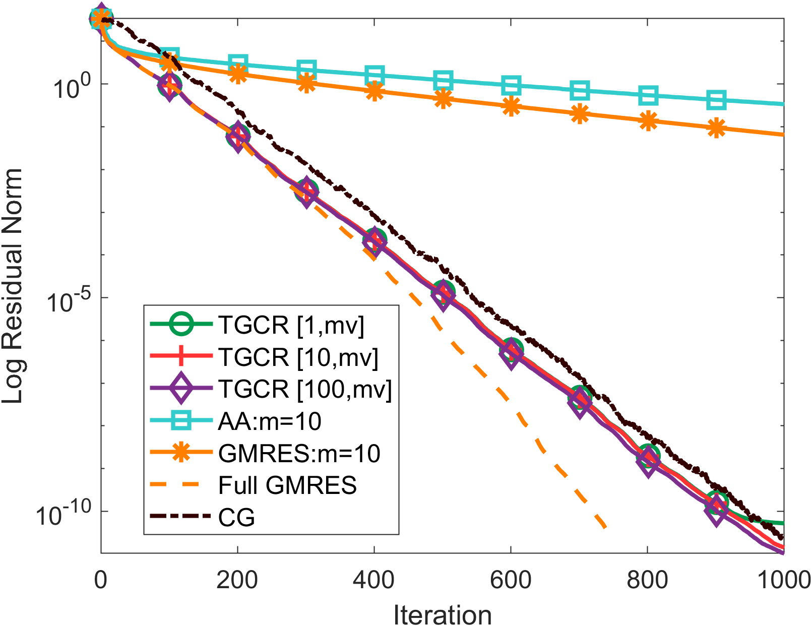
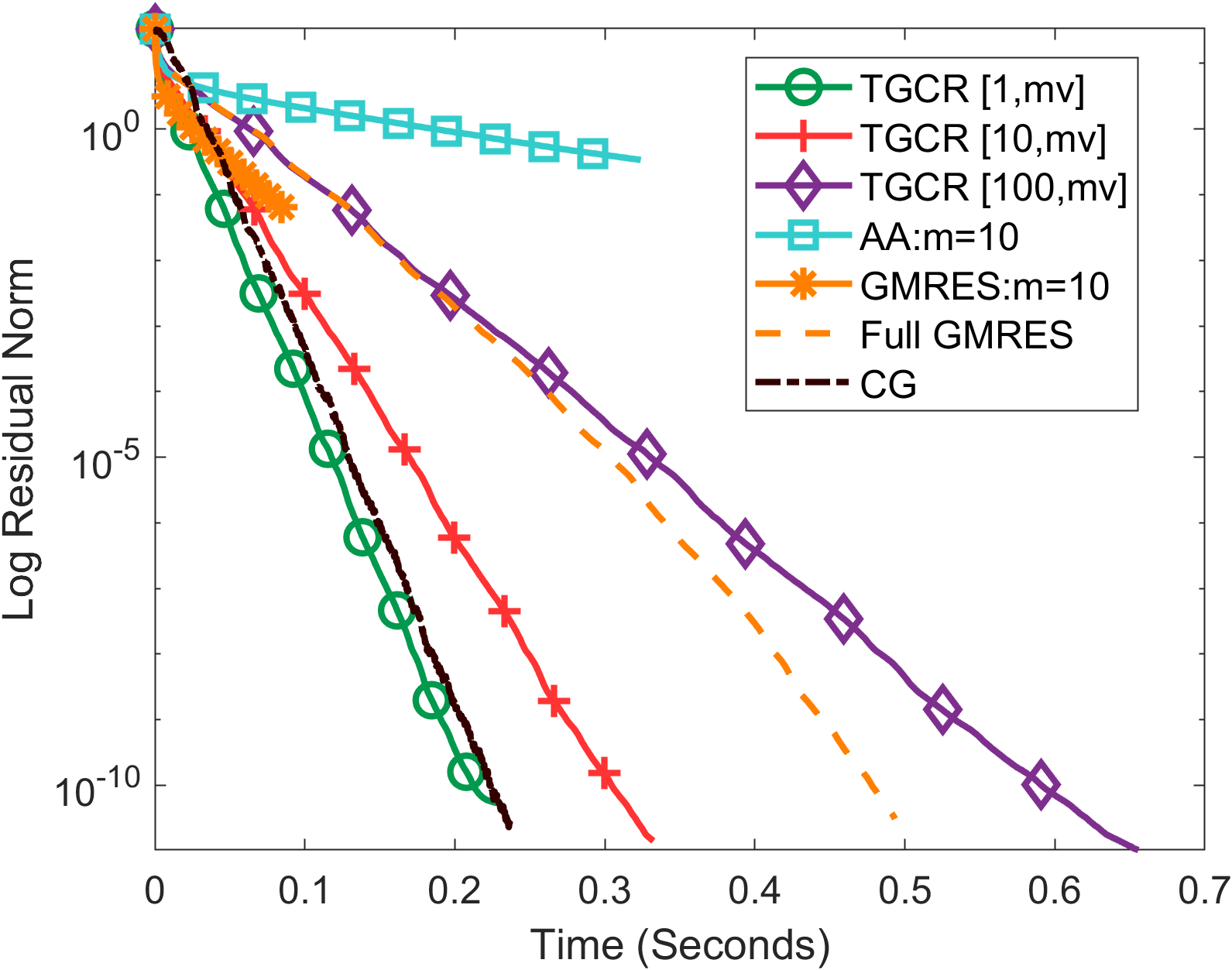
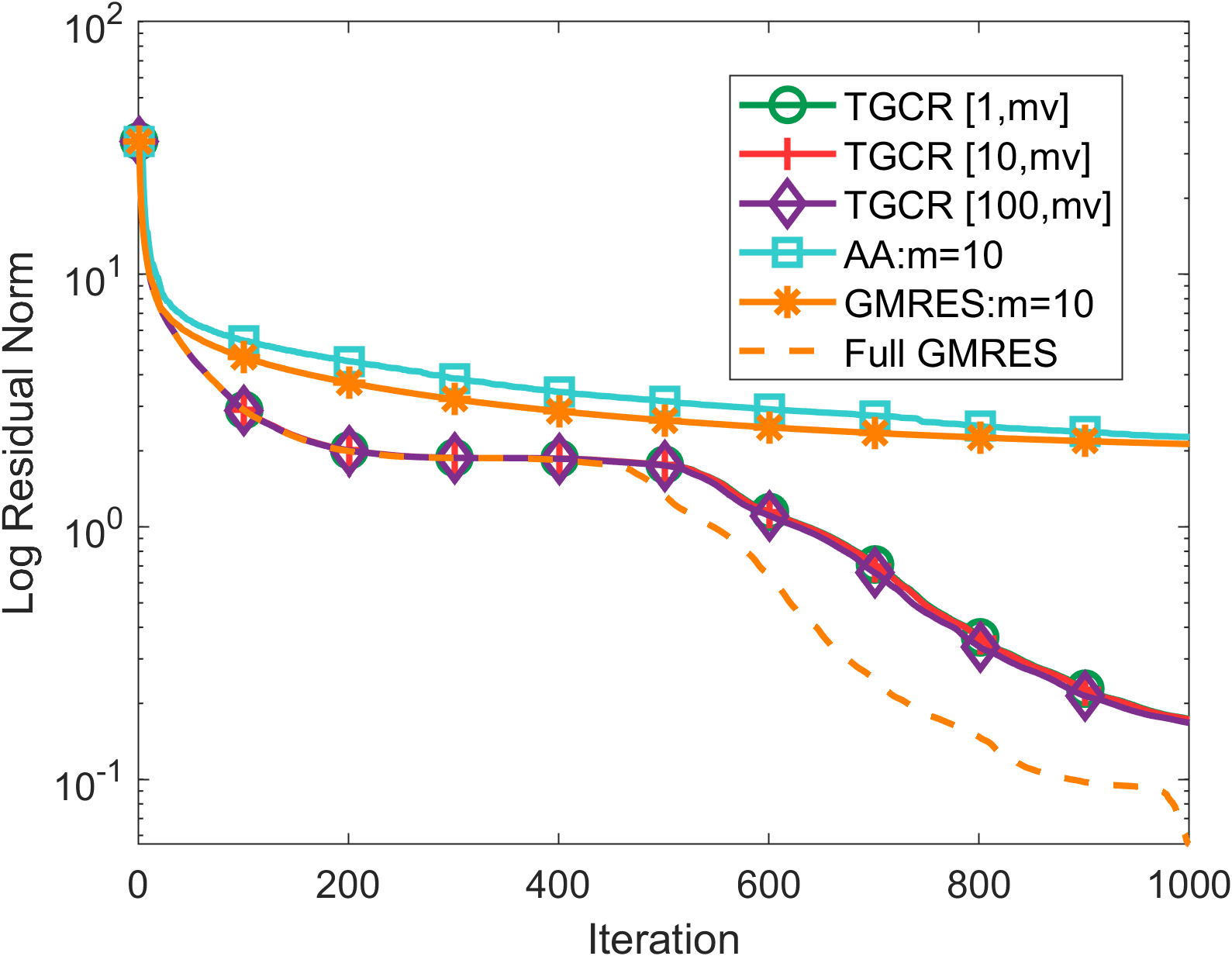
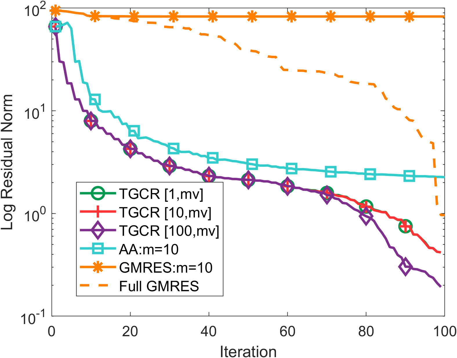
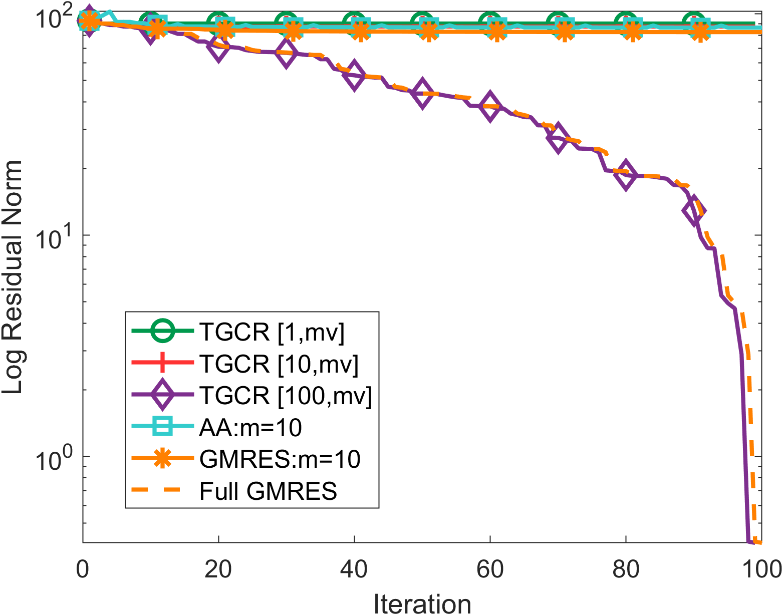
The advantages of TGCR for linear systems are two-folds. 1:) Theorem 11 shows that TGCR () is already optimal (equivalent to Conjugate Residual) when is symmetric positive definite. A larger table size is unnecessary while AA and GMRES require more past iterates to converge fast. It can be observed from Figure 1(a) and 1(b) that TGCR () requires much less memory and computation overhead to converge compared to GMRES and AA. It also has the same convergence behavior and similar running time as CG. 2:) It is easy to show that TGCR can converge for indefinite systems while CG fails. Figure 1(c) verifies our point. This can be helpful when it is not known in advance if the system is indefinite. The numerical results shown in Figure 1 demonstrate the power of TGCR as a variant of Krylov subspace methods. Figure 1 clearly verifies the correctness of Theorem 11 that TGCR (1) is identical with TGCR in exact arithmetic, which leads to big savings both in terms of memory and in computational costs. We include more experimental results in the Appendix C.2.
4.2 Nonlinear Problems: Softmax Classification
Next, we consider a softmax multi-class classification problem shown in (79) without regularization.
| (23) |
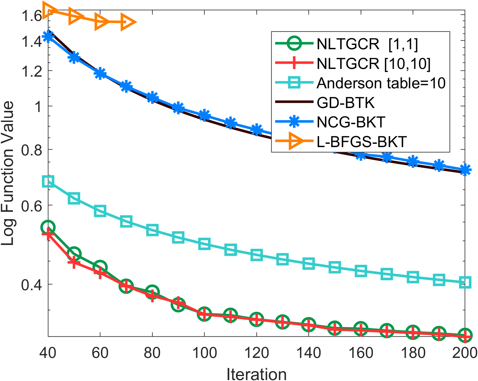
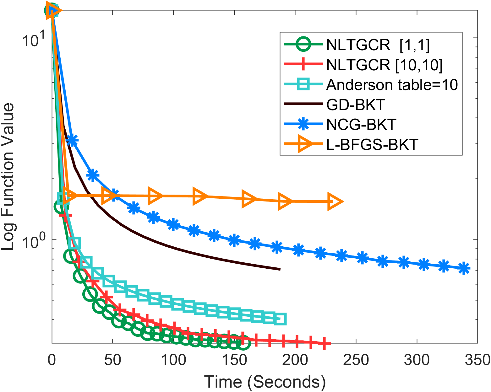
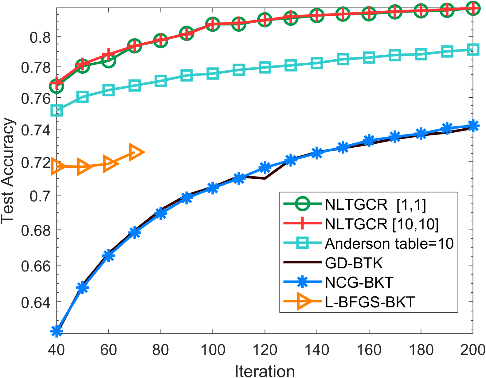
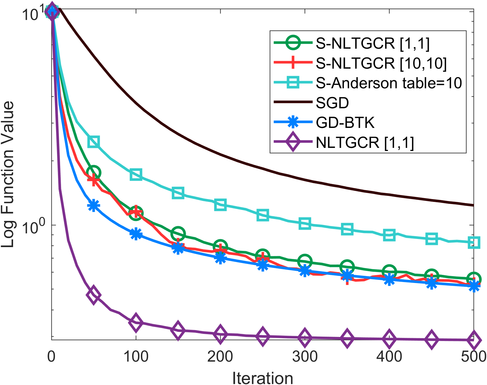
where is the total number of sample, is the total number of classes, is vector of all features of sample , is the weights for the class, and is the correct class for the sample. We compare nlTGCR with Gradient Descent (GD), Nonlinear Conjugate Gradient (NCG) [13], L-BFGS [38] and Anderson Acceleration using the MNIST dataset [16] and report results in Figure 2. Figure 2(a) and 2(b) plot the objective value vs. iteration number and wall-clock time respectively. It can be seen that nlTGCR converges significantly faster than baselines even without a line-search strategy. In addition, for this convex and symmetric problem, it is not surprising to observe that nlTGCR exhibits a similar convergence rate with nlTGCR, which saves even more memory and computation time. Figure 2(c) shows that nlTGCR greatly outperforms baselines by achieving high test accuracy in the very early stage of training. Figure 2(d) shows the effectiveness of our method in the stochastic setting. ‘S-’ stands for a stochastic version. We use a step size of 0.2 for SGD and a batch size () of 500 for all stochastic algorithms. It can be observed that nlTGCR(1) with a small batch size is comparable with the full batch GD with line-search, which confirms that TGCR takes advantage of symmetry in a very effective way even in the case of stochastic gradients.
4.3 Deep learning applications
We then evaluate nlTCGR on several widely-used deep learning applications using different frameworks. We run experiments on image classification using CNN [42] and ResNet [27], time series forecasting using LSTM [31], and node classification using GCN [35]. Due to space limitation, we provide full results in Appendix C.5. It shows that nlTGCR(1) outperforms baselines (SGD, Nesterov, and Adam) for the above DL experiments, highlighting its effectiveness in large-scale and stochastic non-convex optimization.
5 Conclusion
This paper describes an efficient nonlinear acceleration method that takes advantage of the symmetry of the Hessian. We studied the convergence properties of the proposed method and established a few connections with existing methods. The numerical results suggest that nlTGCR can be a competitive iterative algorithm from both theoretical and practical perspectives. We plan to conduct a more detailed theoretical and experimental investigation of the method for a nonconvex stochastic setting.
Social Impact. This work does not present any foreseeable societal consequence.
References
- [1] D. G. Anderson. Iterative procedures for non-linear integral equations. Assoc. Comput. Mach., 12(547):547–560, 1965.
- [2] W. Azizian, I. Mitliagkas, S. Lacoste-Julien, and G. Gidel. A tight and unified analysis of gradient-based methods for a whole spectrum of games, 2019.
- [3] C. Blair. Problem complexity and method efficiency in optimization (a. s. nemirovsky and d. b. yudin). SIAM Review, 27(2):264–265, 1985.
- [4] R. Bollapragada, R. Byrd, and J. Nocedal. Exact and inexact subsampled newton methods for optimization, 2016.
- [5] R. Bollapragada, R. H. Byrd, and J. Nocedal. Exact and inexact subsampled newton methods for optimization. IMA Journal of Numerical Analysis, 39(2):545–578, 2019.
- [6] N. Boutet, R. Haelterman, and J. Degroote. Secant update version of quasi-newton psb with weighted multisecant equations. Computational Optimization and Applications, 75(2):441–466, 2020.
- [7] N. Boutet, R. Haelterman, and J. Degroote. Secant update generalized version of psb: a new approach. Computational Optimization and Applications, 78(3):953–982, 2021.
- [8] C. Brezinski and M. Redivo-Zaglia. The simplified topological -algorithms for accelerating sequences in a vector space. SIAM Journal on Scientific Computing, 36(5):A2227–A2247, 2014.
- [9] C. Brezinski, M. Redivo-Zaglia, and Y. Saad. Shanks sequence transformations and anderson acceleration. SIAM Review, 60(3):646–669, 2018.
- [10] P. N. Brown and Y. Saad. Hybrid Krylov methods for nonlinear systems of equations. SIAM J. Sci. Stat. Comp., 11:450–481, 1990.
- [11] P. N. Brown and Y. Saad. Convergence theory of nonlinear Newton-Krylov algorithms. SIAM Journal on Optimization, 4:297–330, 1994.
- [12] S. Cabay and L. W. Jackson. A polynomial extrapolation method for finding limits and antilimits of vector sequences. SIAM Journal on Numerical Analysis, 13(5):734–752, 1976.
- [13] Y. H. Dai and Y. Yuan. A nonlinear conjugate gradient method with a strong global convergence property. SIAM Journal on Optimization, 10(1):177–182, 1999.
- [14] A. d’Aspremont, D. Scieur, and A. Taylor. Acceleration methods. Foundations and Trends® in Optimization, 5(1-2):1–245, 2021.
- [15] R. S. Dembo, S. C. Eisenstat, and T. Steihaug. Inexact Newton methods. SIAM J. Numer. Anal., 18(2):400–408, 1982.
- [16] L. Deng. The mnist database of handwritten digit images for machine learning research. IEEE Signal Processing Magazine, 29(6):141–142, 2012.
- [17] J. E. Dennis and J. J. Moré. Quasi-newton methods, motivation and theory. SIAM Rev., 19:46–89, 1977.
- [18] M. Derezinski, J. Lacotte, M. Pilanci, and M. W. Mahoney. Newton-LESS: Sparsification without trade-offs for the sketched newton update. In A. Beygelzimer, Y. Dauphin, P. Liang, and J. W. Vaughan, editors, Advances in Neural Information Processing Systems, 2021.
- [19] S. C. Eisenstat, H. C. Elman, and M. H. Schultz. Variational iterative methods for nonsymmetric systems of linear equations. SIAM Journal on Numerical Analysis, 20:345–357, 1983.
- [20] S. C. Eisenstat and H. F. Walker. Globally convergent inexact newton methods. SIAM Journal on Optimization, 4:393–422, 1994.
- [21] V. Eyert. A comparative study on methods for convergence acceleration of iterative vector sequences. J. Computational Phys., 124:271–285, 1996.
- [22] M. Geist and B. Scherrer. Anderson acceleration for reinforcement learning, 2018.
- [23] D. Goldfarb, Y. Ren, and A. Bahamou. Practical quasi-newton methods for training deep neural networks. In Proceedings of the 34th International Conference on Neural Information Processing Systems, NIPS’20, Red Hook, NY, USA, 2020. Curran Associates Inc.
- [24] W. W. Hager and H. Zhang. A survey of nonlinear conjugate gradient methods. 2005.
- [25] H. He, S. Zhao, Y. Xi, J. Ho, and Y. Saad. GDA-AM: ON THE EFFECTIVENESS OF SOLVING MIN-IMAX OPTIMIZATION VIA ANDERSON MIXING. In International Conference on Learning Representations, 2022.
- [26] H. He, S. Zhao, Y. Xi, J. C. Ho, and Y. Saad. Solve minimax optimization by anderson acceleration, 2021.
- [27] K. He, X. Zhang, S. Ren, and J. Sun. Deep residual learning for image recognition. arXiv preprint arXiv:1512.03385, 2015.
- [28] K. He, X. Zhang, S. Ren, and J. Sun. Deep residual learning for image recognition, 2015.
- [29] M. R. Hestenes and E. Stiefel. Methods of conjugate gradients for solving linear systems. Journal of research of the National Bureau of Standards, 49:409–435, 1952.
- [30] N. J. Higham and N. Strabi. Anderson acceleration of the alternating projections method for computing the nearest correlation matrix. to appear.
- [31] S. Hochreiter and J. Schmidhuber. Long short-term memory. Neural Computation, 1997.
- [32] S. Hochreiter and J. Schmidhuber. Long short-term memory. Neural computation, 9:1735–80, 12 1997.
- [33] K. Jbilou and H. Sadok. Lu implementation of the modified minimal polynomial extrapolation method for solving linear and nonlinear systems. IMA Journal of Numerical Analysis, 19(4):549–561, 1999.
- [34] C. T. Kelley. Newton’s method in mixed precision. SIAM Review, 64(1):191–211, 2022.
- [35] T. N. Kipf and M. Welling. Semi-supervised classification with graph convolutional networks. In International Conference on Learning Representations (ICLR), 2017.
- [36] T. N. Kipf and M. Welling. Semi-Supervised Classification with Graph Convolutional Networks. arXiv:1609.02907 [cs, stat], Feb. 2017. arXiv: 1609.02907.
- [37] A. Krizhevsky. Learning multiple layers of features from tiny images. 2009.
- [38] D. C. Liu and J. Nocedal. On the limited memory bfgs method for large scale optimization. Mathematical Programming, 45:503–528, 1989.
- [39] V. V. Mai and M. Johansson. Nonlinear acceleration of constrained optimization algorithms. In ICASSP 2019 - 2019 IEEE International Conference on Acoustics, Speech and Signal Processing (ICASSP), pages 4903–4907, 2019.
- [40] J. Martens. Deep learning via hessian-free optimization. In Proceedings of the 27th International Conference on International Conference on Machine Learning, ICML’10, page 735–742, Madison, WI, USA, 2010. Omnipress.
- [41] P. Ni. Anderson Acceleration of Fixed-point Iteration with Applications to Electronic Structure Computations. PhD thesis, Worcester Polytechnic Institute, Worcester, Massachusetts, USA, 2009.
- [42] K. O’Shea and R. Nash. An introduction to convolutional neural networks, 2015.
- [43] W. Ouyang, Y. Liu, and A. Milzarek. Descent properties of an anderson accelerated gradient method with restarting. 06 2022.
- [44] M. L. Pasini, J. Yin, V. Reshniak, and M. K. Stoyanov. Anderson acceleration for distributed training of deep learning models. In SoutheastCon 2022, pages 289–295, 2022.
- [45] M. POWELL. A new algorithm for unconstrained optimization. In J. Rosen, O. Mangasarian, and K. Ritter, editors, Nonlinear Programming, pages 31–65. Academic Press, 1970.
- [46] H. ren Fang and Y. Saad. Two classes of multisecant methods for nonlinear acceleration. Numerical Linear Algebra with Applications, 16(3):197–221, 2009.
- [47] F. Roosta, Y. Liu, P. Xu, and M. W. Mahoney. Newton-mr: Inexact newton method with minimum residual sub-problem solver, 2018.
- [48] F. Roosta-Khorasani and M. W. Mahoney. Sub-sampled newton methods i: Globally convergent algorithms, 2016.
- [49] C. W. Royer, M. O’Neill, and S. J. Wright. A newton-cg algorithm with complexity guarantees for smooth unconstrained optimization. Math. Program., 180(1–2):451–488, mar 2020.
- [50] Y. Saad. Numerical Methods for Large Eigenvalue Problems. Halstead Press, New York, 1992.
- [51] Y. Saad. Iterative Methods for Sparse Linear Systems, 2nd edition. SIAM, Philadelpha, PA, 2003.
- [52] Y. Saad and M. H. Schultz. GMRES: a generalized minimal residual algorithm for solving nonsymmetric linear systems. SIAM Journal on Scientific and Statistical Computing, 7:856–869, 1986.
- [53] R. B. Schnabel. Quasi-newton methods using multiple secant equations. Technical Report CU-CS-247-83, Department of Computer Science, University of Colorado at Boulder, Boulder, CO, 1983.
- [54] D. Scieur, L. Liu, T. Pumir, and N. Boumal. Generalization of quasi-newton methods: Application to robust symmetric multisecant updates, 2020.
- [55] D. Scieur, L. Liu, T. Pumir, and N. Boumal. Generalization of quasi-newton methods: Application to robust symmetric multisecant updates. In A. Banerjee and K. Fukumizu, editors, Proceedings of The 24th International Conference on Artificial Intelligence and Statistics, volume 130 of Proceedings of Machine Learning Research, pages 550–558. PMLR, 13–15 Apr 2021.
- [56] D. Scieur, E. Oyallon, A. d’Aspremont, and F. Bach. Online regularized nonlinear acceleration, 2018.
- [57] W. Shi, S. Song, H. Wu, Y. Hsu, C. Wu, and G. Huang. Regularized anderson acceleration for off-policy deep reinforcement learning. In NeurIPS, 2019.
- [58] D. A. Smith, W. F. Ford, and A. Sidi. Extrapolation methods for vector sequences. SIAM Review, 29(2):199–233, 1987.
- [59] H. D. Sterck and Y. He. On the asymptotic linear convergence speed of anderson acceleration, nesterov acceleration, and nonlinear gmres. SIAM Journal on Scientific Computing, 43(5):S21–S46, 2021.
- [60] K. Sun, Y. Wang, Y. Liu, Y. Zhao, B. Pan, S. Jui, B. Jiang, and L. Kong. Damped anderson mixing for deep reinforcement learning: Acceleration, convergence, and stabilization. In NeurIPS, 2021.
- [61] H. F. Walker and P. Ni. Anderson acceleration for fixed-point iterations. SIAM J. Numer. Anal., 49(4):1715–1735, 2011.
- [62] F. Wei, C. Bao, and Y. Liu. Stochastic anderson mixing for nonconvex stochastic optimization, 2021.
- [63] F. Wei, C. Bao, and Y. Liu. A class of short-term recurrence anderson mixing methods and their applications. In International Conference on Learning Representations, 2022.
- [64] Y. Xie, R. H. Byrd, and J. Nocedal. Analysis of the bfgs method with errors. SIAM Journal on Optimization, 30(1):182–209, 2020.
- [65] Z. Yao, A. Gholami, S. Shen, M. Mustafa, K. Keutzer, and M. W. Mahoney. Adahessian: An adaptive second order optimizer for machine learning. 2020.
- [66] G. Zhang and Y. Yu. Convergence of gradient methods on bilinear zero-sum games. In ICLR, 2020.
- [67] J. Zhang, B. O’Donoghue, and S. Boyd. Globally convergent type-i anderson acceleration for non-smooth fixed-point iterations, 2018.
- [68] J. Zhang, B. O’Donoghue, and S. Boyd. Globally convergent type-i anderson acceleration for nonsmooth fixed-point iterations. SIAM Journal on Optimization, 30(4):3170–3197, 2020.
Appendix A Additional Discussion
A.1 High-Level Clarification
The method described in this paper mixes a number of ideas coming from different horizons. Some of the high-level discussion provided below is expanding further in later sections.
Linear case: TGCR. Our initial idea was motivated by considering the linear case, in an attempt to exploit Conjugate-gradient like methods for solving a linear system . When is symmetric, it is known that it is possible to minimize the objective function on the -th Krylov subspace by a nice algorithm that uses a short-term recurrence. This algorithm, called the Conjugate Residual algorithm, is quite similar to the Conjugate Gradient but its residual vectors are conjugate (instead of being orthogonal) and its search directions are conjugate (instead of being -conjugate). Its generalization to the nonsymmetric case, called the Generalized Conjugate Residual method, is easy to obtain by enforcing these two properties. Enforcing the conjugacy of the ’s is the same as enforcing the orthogonality of the vectors and this is expensive when we have many vectors. For this reason, practical versions of the algorithm are truncated, i.e., the orthogonalization is enforced against only a few previous directions. The result is the TGCR(m) algorithm (Algorithm 1) – which has been known since the 1980s. It is clear that we expect that when the matrix is nearly symmetric TGCR(m) will perform nearly as well as the full version GCR - because when is symmetric, taking will yield full orthogonality of the s (Theorem B.2).
Nonlinear case: Newton Krylov. Suppose now that we have to solve the nonlinear system (in optimization is just the gradient of the objective function). At this point, we may ask the question: why not just use an inexact Newton method whereby the Jacobian system is solved with the linear GCR or TGCR method? This is where Anderson acceleration provides an interesting insight on some weaknesses of Newton-Krylov method. A Newton Krylov method generates a Krylov subspace at a current iterate – say – (so ) and tries to minimize where , by exploiting the linear model: . If we generate a basis of and express as then we would need to minimize which is a small least-squares problem. One usually adds to this a global convergence strategies, e.g., a linesearch or a trust-region technique to produce the next iterate . The problem with this approach is this: the approximate solution obtained after steps of a Krylov subspace approach is based on the Jacobian at the initial point . The intermediate calculation is entirely linear and based on . It is not exploited in any way to produce intermediate (nonlinear) iterates which in turn could be used to produce more accurate information on some local Jacobian. In contrast, a method like Anderson acceleration (or in fact any of the secant or multisecant methods) will do just this, i.e., it will tend to use information on the nonlinear mapping near the most recent approximation to produce the new iterate. This distinction is rather important although if the problem is nearly linear, then it could make little difference.
Nonlinear case: Anderson and nlTGCR. Anderson acceleration can be viewed as a form of Quasi-Newton method whereby the approximate inverse Jacobian is updated at each step by using the collection of the previous iterates and the corresponding function values . To be more accurate it uses the differences and the corresponding defined in the same way. Similarly to Newton-Krylov, it generates an approximation of the form where is a basis of the subspace spanned by the ’s. Notice how the update now is on the latest point generated. The previous iterates are used to essentially provide information on the nonlinear mapping and its differential. This information is constantly updated using the most recent iterate. Note that this is informally stated: Anderson does not formally get an approximation to the Jacobian. It is based implicitly on exploiting the relation . Herein lies a problem that nlTGCR aims at correcting: this relation is only vaguely verified. For example, if we take to be , the Jacobian at , the resulting linear model is bound to be extremely inaccurate at the beginning of the iteration.
In nlTGCR, we try to improve on the Newton-Krylov approach, since our starting point is TGCR which is generalized to nonlinear problems. We also take the viewpoint of improving on Anderson Acceleration or multisecant methods by not relying on the approximation mentioned above. This is achieved by adopting the projection viewpoint. Instead of minimizing as in the inexact Newton mode, we would like to now minimize where is the most recent iterate. This initial idea leads to a difficulty since there is not one but several ones at previous points and a single one of them will not be satisfactory. Thus, we have a few directions just like the differences in Anderson, but now each will lead to a which - unlike in AA - is accurately computed and then saved. This feature is what we believe makes a difference in the performance of the algorithm – although this is something that would be rather difficult to prove theoretically.
The Quasi-Newton viewpoint.. It is also possible to view the algorithm from the alternative angle of a Quasi-Newton approach instead of Inexact Newton. In this viewpoint, the inverse of the Jacobian is approximated progressively. Because it is the inverse Jacobian that is approximated, the method is akin to Broyden’s second update method.
In our case, the approximate inverse Jacobian at step is equal to
| (24) |
If we apply this to the vector we get So inverts exactly when applied to . It therefore satisfies the secant equation ([46, sec. 2.3])
| (25) |
This is the equivalent to the secant condition used in Broyden’s second update method. Broyden type-II methods replace Newtons’s iteration: with where approximates the inverse of the Jacobian at by the update formula in which is defined in different ways see [46] for details.
In addition, the update satisfies the ‘no-change’ condition:
| (26) |
The usual no-change condition for secant methods is of the form for which in our case would be for . One can therefore consider that we are updating .
It is also possible to find a link between the method proposed herein and the Anderson acceleration, by unraveling a relation with multi-secant methods. Note that equation (25) is satisfied for (at most) previous instances of , i.e., at step we have ( defined in the algorithm) for In other words we can also write
| (27) |
This is similar to the multi-secant condition of Equation (7) – see also equation (13) of [46] where and are defined in (2). In addition, we clearly also have a multi secant version of the no-change condition (26) seen above, which becomes:
| (28) |
This is similar to the no-change condition represented by eq. (15) of [46], which stipulates that for all orthogonal to the span of the subspace mentioned above, provided we define .
A.2 Complexity Analysis
Assume that the iteration number is and the model parameter size is . The full memory AA stores all previous iterations, thus the additional memory is . To reduce the memory overhead, the limited-memory (Truncated) AA maintains the most recent iterations while discarding the older historical information. In comparison, TGCR and NLTGCR only requires the most recent iterate to achieve optimal performance, thus the additional memory is . The reduced number of past iterates also saves the orthogonalization costs from TGCR and NLTGCR compared to AA(m). In TGCR and NLTGCR, only one orthogonalization is needed to performed which costs while AA(m) requires .
For TGCR(m), flops are performed in Line 5, flops are performed in Lines 6-7 and flops are performed in the for loop and flops are performed in Line 15. If TGCR(m) performs k iterations, the computational complexity is . Thus, TGCR costs . For symmetric problems, is guaranteed to generate the same iterates as and TGCR costs .
Then we analyze the complexity of nlTGCR(m). flops are performed in Line 6, flops are performed in Line 7, two evaluations of are performed in Lines 8 and 11. The for loop costs flops and flops are performed in Line 15. When iterations are performed, nlTGCR costs plus the costs of function evaluations of . When is used in nonlinear problems, nlTGCR costs plus the costs of function evaluations of .
A.3 The Frechet derivative
In vector analysis, derivatives provide local linear approximations. Frechet differentiation can be used to calculate directional derivatives of gradients. We use Frechet Differentiation to compute the directional derivative of a gradient mapping at in direction , which is in algorithm 2. We define Frechet derivative as follows,
Definition 1.
Let and be two normed spaces and let be an open set in .
A function is Fréchet differentiable at , where , if there exists a linear operator such that
The operator is referred to the Fréchet derivative at .
Appendix B Proofs
B.1 Optimality for Linear Problem
We can write the Generalized Conjugate residual formally as follows
Theorem B.1 (Lemma 6.21 in [51].).
If is the basis of the Krylov space which are also orthogonal . Then
minimizes the residual among all the iterates with form . Further more, we have
Proof.
We can write and . Since minimizes the residual, we know the following Petrov–Galerkin condition must hold
The orthogonality gives us
Similarly, we can write and . Agagin, the optimality condition reads
which gives us
∎
Theorem B.2.
When the coefficient matrix is symmetric, TGCR(m) generates exactly the same iterates as TGCR(1) for any .
Proof.
Lines 8 to 14 in Algorithm 1 computes the new direction – by ortho-normalizing the vector against all previous ’s. In fact the loop of lines 9–13, implements a modified Gram-Schmidt procedure, which in exact arithmetic amounts simply to setting to
| (29) |
In the above relation, is the scaling factor used to normalize and in Line 14. Then, is computed accordingly as is reflected in lines 12 and 14. The update relation (from Line 12) shows that for . In addition, it can easily be shown that in this case () the residual vectors produced by the algorithm are -conjugate in that for . Indeed, this requires a simple induction argument exploiting the equality:
and relation (29) which shows that .
When is symmetric, exploiting the relation , we can see that the scalar in Line 11 of Algorithm 1 is
which is equal to zero for . Therefore we need to orthogonalize against vector only in the loop of lines 9 to 13. This completes the proof. ∎
Theorem B.3.
Let be the approximate solution obtained at the t-th iteration of TGCR being applied to solve , and denote the residual as . Then, is of the form
| (30) |
where
| (31) |
where is the family of polynomials with degree p such that , which are usually called residual polynomials.
Theorem B.4 (Convergence of TGCR (Indefinite Case)).
Suppose is hermitian, invertible, and indefinite. Divide its eigenvalues into positive and negative sets and , and define
Then , the th solution estimate of TGCR, satisfies
where means to round down to the nearest integer.
Proof.
When A is hermitian indefinite, an estimate on the min-max approximation
| (32) |
that represents the worst-case TGCR convergence behavior, can be obtained by replacing the discrete set of the eigenvalues by the union of two intervals containing all of them and excluding the origin, say and . Then the classical bound for the min-max value can be used to obtain an estimate for the convergence of the residual [50]
where denotes the integer part of . ∎
The optimality of TGCR(m) is proved in Theorem B.5.
Theorem B.5.
Let be the residual generated by the basic TGCR (m), the following relations hold:
-
1.
-
2.
If , the set of vectors is orthonormal.
-
3.
More generally: for
-
4.
If , then
Proposition 3.
Assume that is nonsingular and that . Then is a descent direction for the function at .
Proof.
It is known [11] that the gradient of at is . In order for to be a descent direction at it is sufficient that the inner product of and is negative. Consider this inner product
| (33) |
which proves the result. ∎
B.2 Optimality from Quasi-Newton Viewpoint
Theorem B.6 (Optimality of nltgcr(m) from Quasi-Newton Viewpoint).
The matrix is the best approximation to the inverse Jacobi of at among all the matrices whose range . That is,
| (34) |
Proof.
Assume is an arbitrary matrix satisfying the multisecant condition . We have and . This can be derived as follows
We also have . Then set , we have
Then we prove . In order to prove this, we compute the trace explicitly. We will denote the natural basis in by and column of by .
Recall we have and , so
∎
B.3 Convergence Analysis
Firstly, we will show the global convergence of the Algorithm 2 from inexact Newton perspective. Usually, some global strategies like line search or residue check are required for inexact Newton method to converge for .
In [11], authors showed with the general line search algorithm 4, inexact Newton-Krylov method can converge globally under some mild conditions.
Theorem B.7 (Global Convergence from Algorithm 2 with linearized update and line search).
Assume is continuously differentiable and is L-lipschitz. Furthre more, the residual check is satisfied where . If is nonsingular and its norm is bounded from above for all n, then produced in line 7 of Algorithm 2 is a descent direction and the iterates produced by Algorithm 2 with linearized update and line search in Algorithm 4 will converge to the minimizer:
Proof.
Theorem B.8 ([11]).
Assume is continuously differentiable and is L-Lipschitz and let be such that for each . Further more, let the next iterate be decided by Algorithm 4 and is nonsingular and bounded from above for all n. Then
The proof of this theorem depends on the following lemma in [11],
Lemma B.9 (Lemma 3.8 of [11]).
Assume is differentiable and is L-lipschitz. Let and denote a descent direction. Then the iterates in Algorithm 4 will generated in finite backtracking steps and satisfies
Theorem B.10 (Global convergence of nlTGCR with residual check).
Assume is twice differentiable and is L-lipschitz. If the residual check is satisfied where and is non-singular and the norm of its inverse is bounded from above for all n, then produced in line 7 of Algorithm 2 is a descent direction and the iterates produced by Algorithm 4 will converge to the minimizer :
Proof.
Denote by , . Since and , we have which implies is a descent direction. To see the second part of the theorem, we have
| (35) | ||||
| (36) |
Denote by then,
Inserting it back to Inequality (27), we have
| (37) |
Denote by and by , then . Since is bounded from below and non-increasing by the inequality. It must converge to a finite limit . If , we ’re done. Otherwise, dividing the Inequality 37 by on both sides, we have
| (38) |
We also know . Therefore, , as . In the above discussion, we showed which implies . Recall , we must have bounded. This contradicts with the fact . Therefore, ∎
To proceed to the superlinear and quadratic convergence results, we need the following lemma from [20]
Lemma B.11.
Assume F is continuously differentiable, is a sequence such that , and for each k,
| (39) |
where and is independent of k. If is a limit point of such that is nonsingular, then and . In this lemma, we don’t require .
Theorem B.12 (Superlinear and quadratic convergence of nlTGCR ).
With the same setting as Theorem B.10. Assume both and are L-Lipschitz. Consider a sequence generated by Algorithm 2 such that residual check is satisfied where . Moreover, if the following conditions hold
| (40) | ||||
| (41) |
for and . If with nonsingular , then . Moreover, there exists such that superlinearly for if , as . Furthermore, if , the convergence is quadratic.
Proof.
In the proof, we denote by for convenience and utilize the proof of Theorem 3.15 in [11]. According to assumptions, with nonsingular, then is nonsingular for for some large enough . Next, if for some , then residual check condition will imply which means for all . Then the results hold automatically because the sequence converges in finite steps. Therefore, we can assume is nonsingular and is nonzero for all .
The residual check condition implies is a descent direction according to Lemma B.9. That is, . Then we can show
To show this notice that according to 40, the following inequality holds
Since is monotone decreasing, thus as . To show . We also need to apply 41. Firstly, according to mean value theorem, there exists a such that
| (42) |
According to 41,
| (43) |
This yields
According to Cauchy-Schwartz inequality,
| (44) |
Therefore,
| (45) |
which means we can draw the conclusion that implies . If with nonsingular, then by Lemma B.11, we know . According to the definition,
| (46) |
This implies
| (47) |
We know as . The above inequality implies that as since is nonsingular. Denote the residual by . Then and . Therefore,
| (48) |
This implies
| (49) |
Since implies , we have
| (50) |
Moreover,
| (51) |
Finally, we have
| (52) |
Using , we have
| (53) |
where . Therefore, we have
| (54) |
This yields,
| (55) |
Hence,
| (56) |
where . Combining 47, we have
| (57) |
where . Next we show the convergence of the algorithm with the aid of the second order Taylor expansion. Notice
| (58) |
The Hessian can be computed as follows
| (59) |
where as since . using second order Taylor expansion, we have
| (60) |
where for some . Then we can have
| (61) | ||||
where . Therefore,
| (62) |
Notice that , and are all bounded from above and , and all converges to as . Therefore as . And choose lager enough such that for all the following holds
| (63) |
Then for all , the Goldsetin-Armijo condition is satisfied,
| (64) |
We then finish the proof following Theorem 3.3 in [15]. It’s easy to see
| (65) |
Taking norm yields
| (66) | ||||
Therefore,
| (67) |
where we used the fact that for sufficient small
| (68) |
which is Lemma 3.1 in [15]. Similarly, to show quadratic convergence, juts notice
| (69) |
for some constant and sufficient small . For more details, check Lemma 3.2 in [15].
∎
B.4 Stochastic nlTGCR
Denote the noisy gradient by and the noisy evaluation of Hessian along a vector by . The subsample exact Newton algorithm is defined in Algorithm 5. At -th iteration, we uniformly subsample from full sample set to estimate the noisy gradient and Hessian, so both of them are unbiased.
Before we start the theoretical analysis, we need to make some assumptions which are usual in stochastic setting.
Assumptions for stochastic setting
-
The eigenvalues of Hessian matrix for any sample is bounded form below and above in Loewner order
(70) Further more, we require there is uniform lower and upper bound for all subsmaples. That is, there exists and such that
(71) And the full Hessian is bounded below and above
(72) -
The variance of subsampled gradients is uniformly bounded by a constant .
(73) -
Hessian is M-Lipschitz, that is
(74) -
The variance of subsampled Hessianis bounded by a constant .
(75) -
There exists a constant such that
Firstly, we recall the few results on subsample Newton method from [5].
Theorem B.13 (Theorem 2.2 in [5]).
Theorem B.14 (Lemma 2.3 form [5]).
Assume is generated by Algorithm 5 with and Assumptions E1-E3 hold. Then
Lemma B.15 (Lemma 2.4 from [5]).
Assume the assumption E1 and E4 hold. Then
| (77) |
Theorem B.16 (Convergence of stochastic version of nlTGCR ).
Assume , residue check is satisfied for and assumptions E1-E5 hold. The iterates generated by the stochastic version Algoritrhm 2 converges to if .
| (78) |
Proof.
The first term can be bounded using the Theorem B.14 and Lemma B.15,
We can bound the second term through the line search, recall at each iteration we have
The last inequality comes from the assumption that eigenvalues of is uniformly upper bounded by . Finally, combining the above inequalities gives us
Taking the total expectation on both sides leads to
We prove the convergence by induction, notice that
Now assume inequality 78 holds for iteration, we prove it for -th iteration
∎
Appendix C Experimental Details and More Experiments
In this section, we first include more experimental details that could not be placed in the main paper due to the space limitation. We then present more experimental results of NLTGCR for different settings and difficult problems.
C.1 Experimental Details
We provide codes implemented in both Matlab and Python. All experiments were run on a Dual Socket Intel E5-2683v3 2.00GHz CPU with 64 GB memory and NVIDIA GeForce RTX 3090.
For linear problems considered in Section 4.1, , and initial points are generated using normally distributed random number. We use to generate symmetric matrices. The step size is set as 1 after rescaling to have the unit 2-norm. For solving linear equations, we depict convergence by use of the norm of residual, which is defined as . For solving bilinear games, we depict convergence by use of the norm of distance to optima, which is defined as . For most baselines, we use the Matlab official implementation.
The softmax regression problem considered in Section 4.2 is defined as follows,
| (79) |
where is the total number of sample, is the total number of classes, is vector of all features of sample , is the weights for the class, and is the correct class for the sample.
C.2 TGCR(1) for linear system
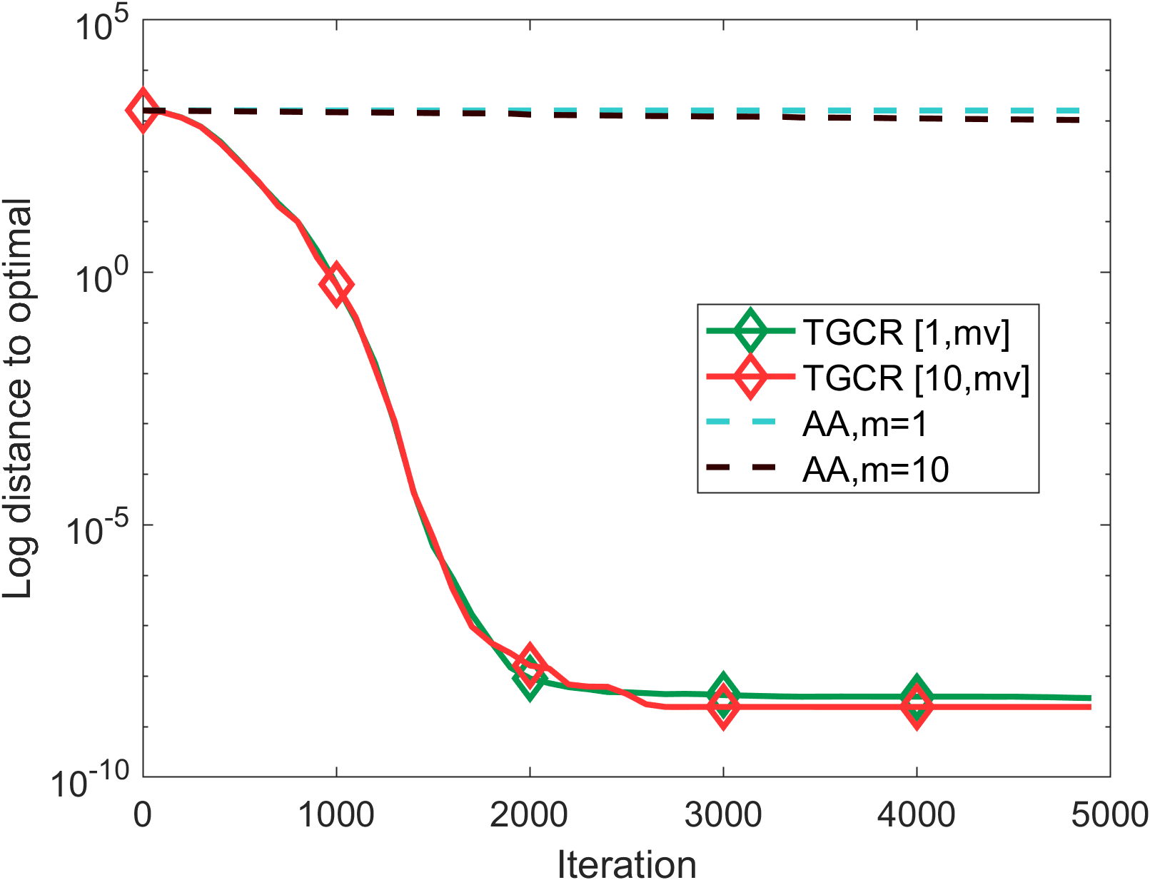
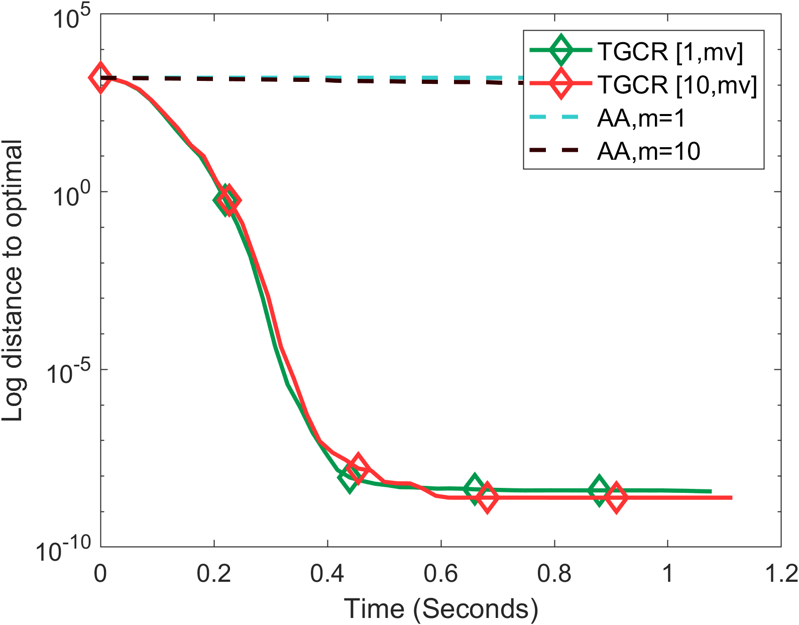
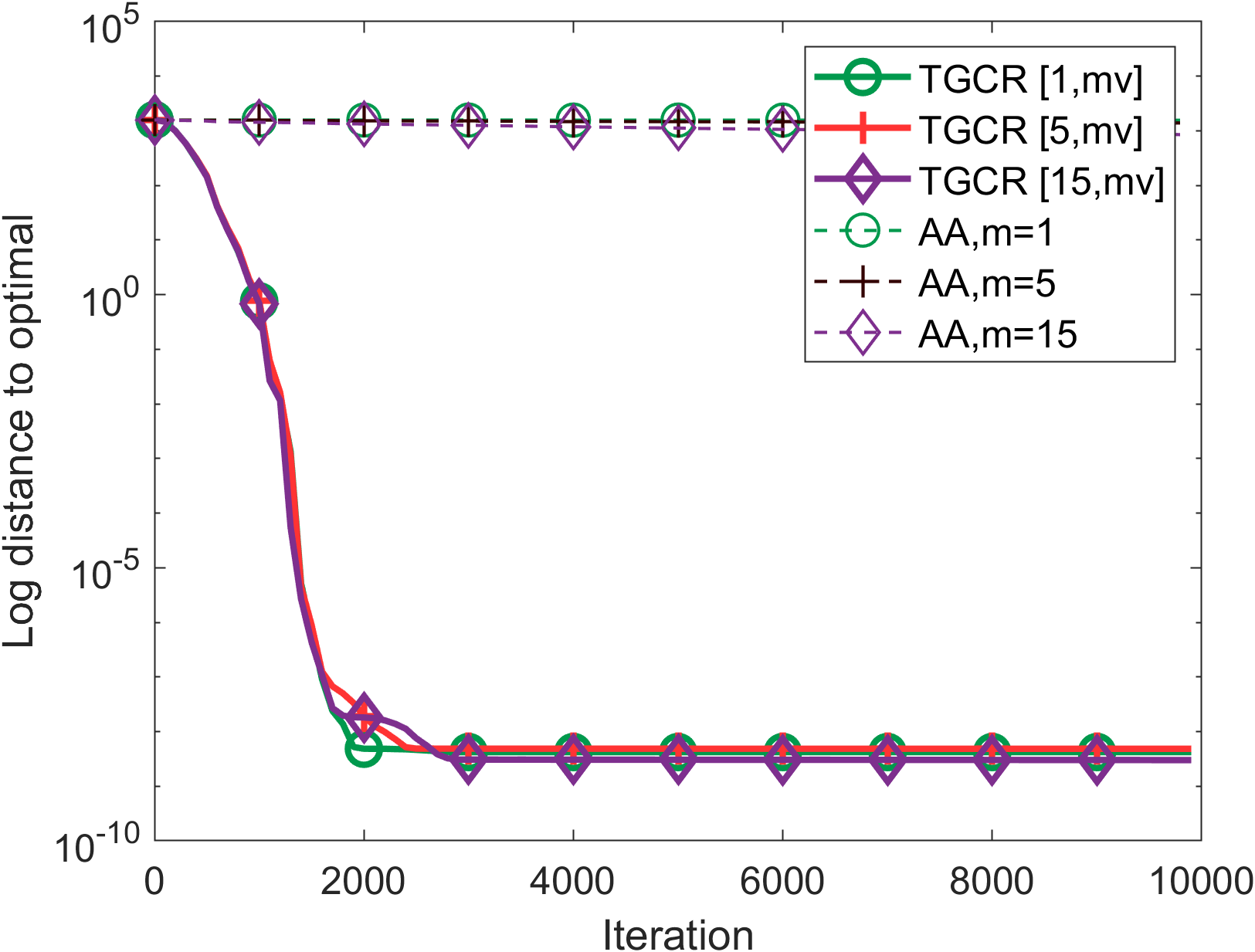
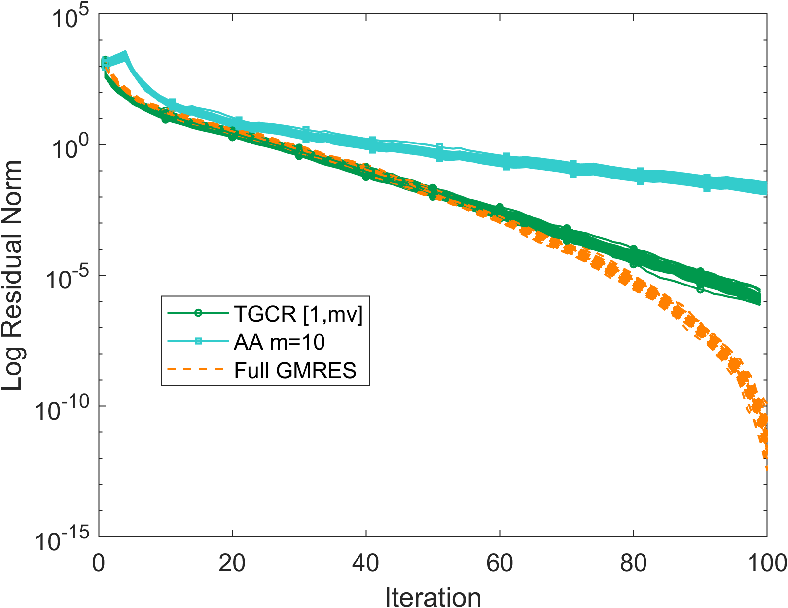
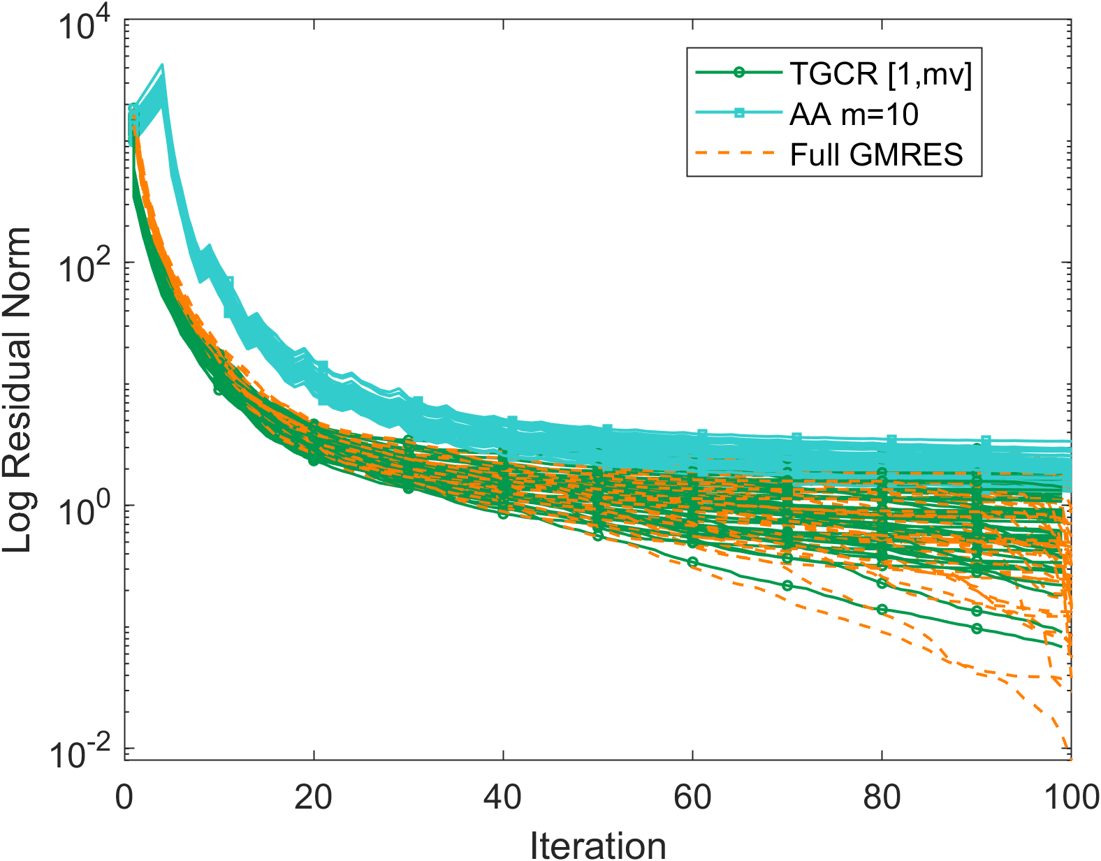
We first test the robustness of TGCR(1) for solving linear systems by running with 50 different initials. Figure 3 indicates TGCR converge well regardless of initialization. We then compare the performance on bilinear games with Anderson Acceleration as [26] shows AA outperforms existing methods on such problems.
Minimax Optimization.
Next, we test TGCR on the following zero-sum bilinear games:
| (80) |
Bilinear games are often regarded as an important but simple class of problems for theoretically analyzing and understanding algorithms for solving general minimax problems [66, 2]. Here we consider simultaneous GDA mapping for minimax bilinear games [26]. Although this mapping is skew-symmetric, TGCR can still exploit the short-term recurrence. It can be observed from Figure 4 that Krylov subspace methods such as TGCR and AA converge fast for bilinear problem when is either SPD or random generated. More importantly, Figure 4 demonstrates that TGCR exhibits a superlinear convergence rate and converges to optimal significantly faster than AA in terms of both iteration number and computation time.
C.3 TGCR(1) for nonsymmetric quadratic minimization and linear system
A quadratic form is simply a scalar, quadratic function of a vector with the form
| (81) |
where is a matrix, and are vectors, and is a scalar constant. When is symmetric and positive-definite, is minimized by the solution to .
C.4 Investigation of Stochastic NLTGCR
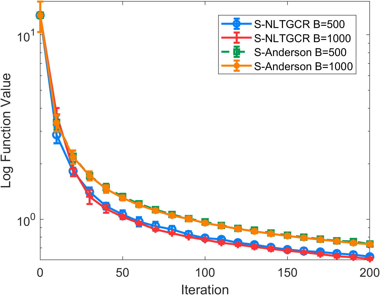
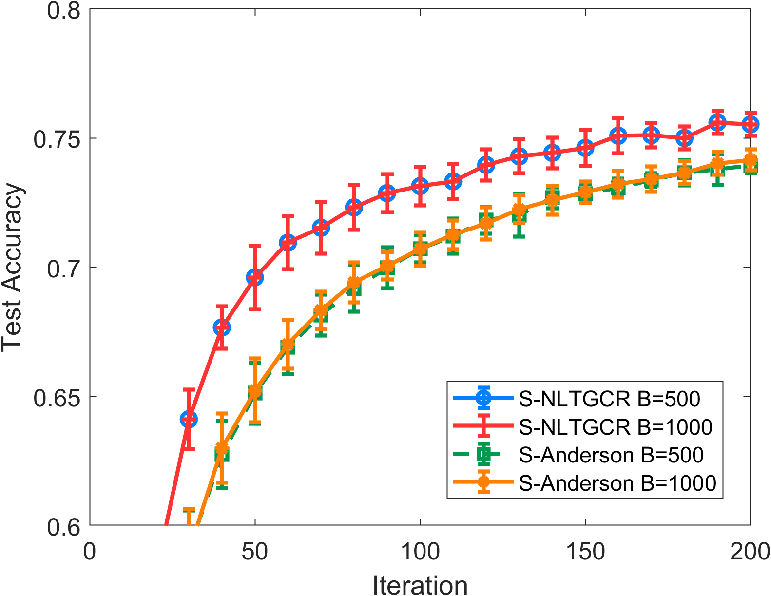
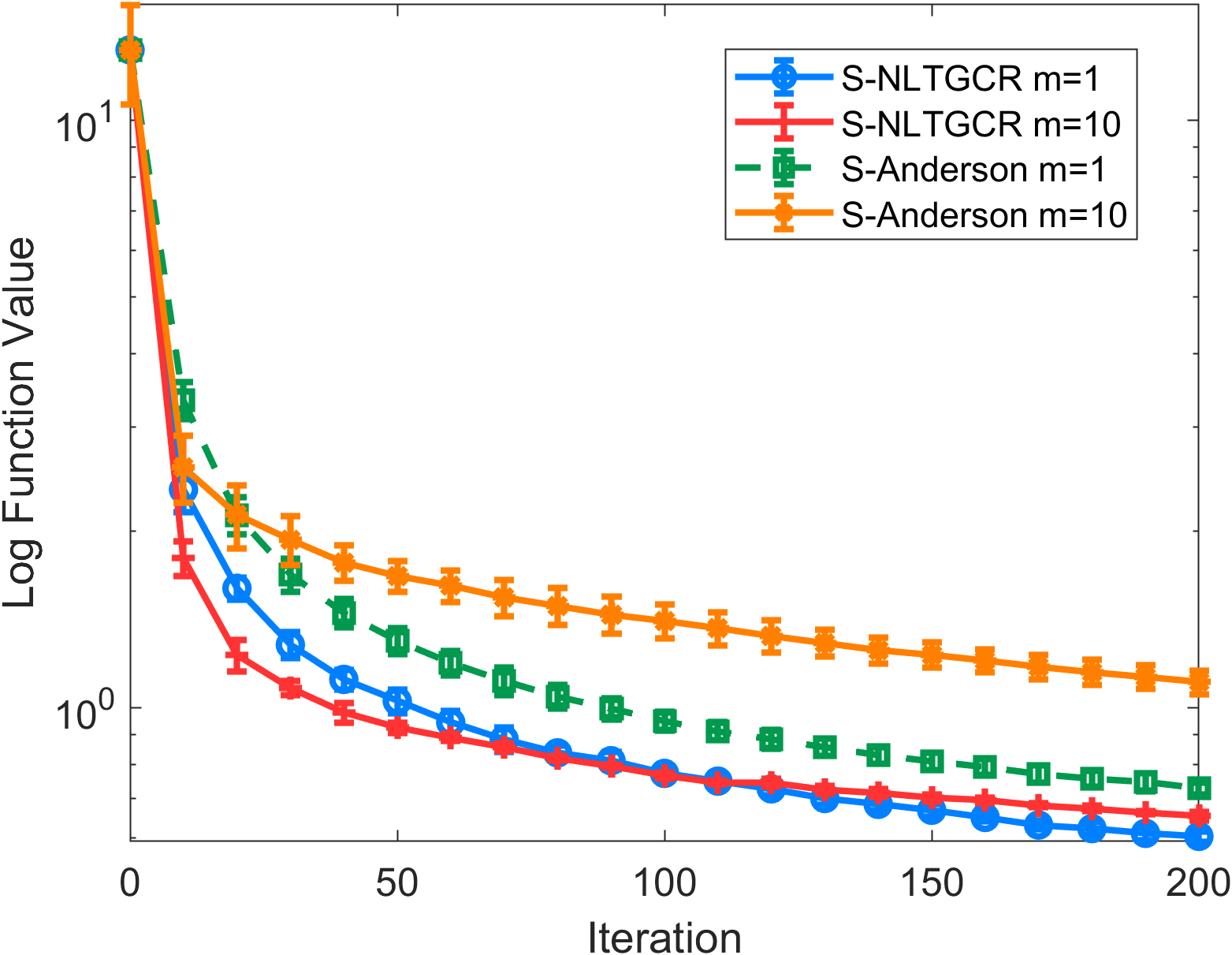
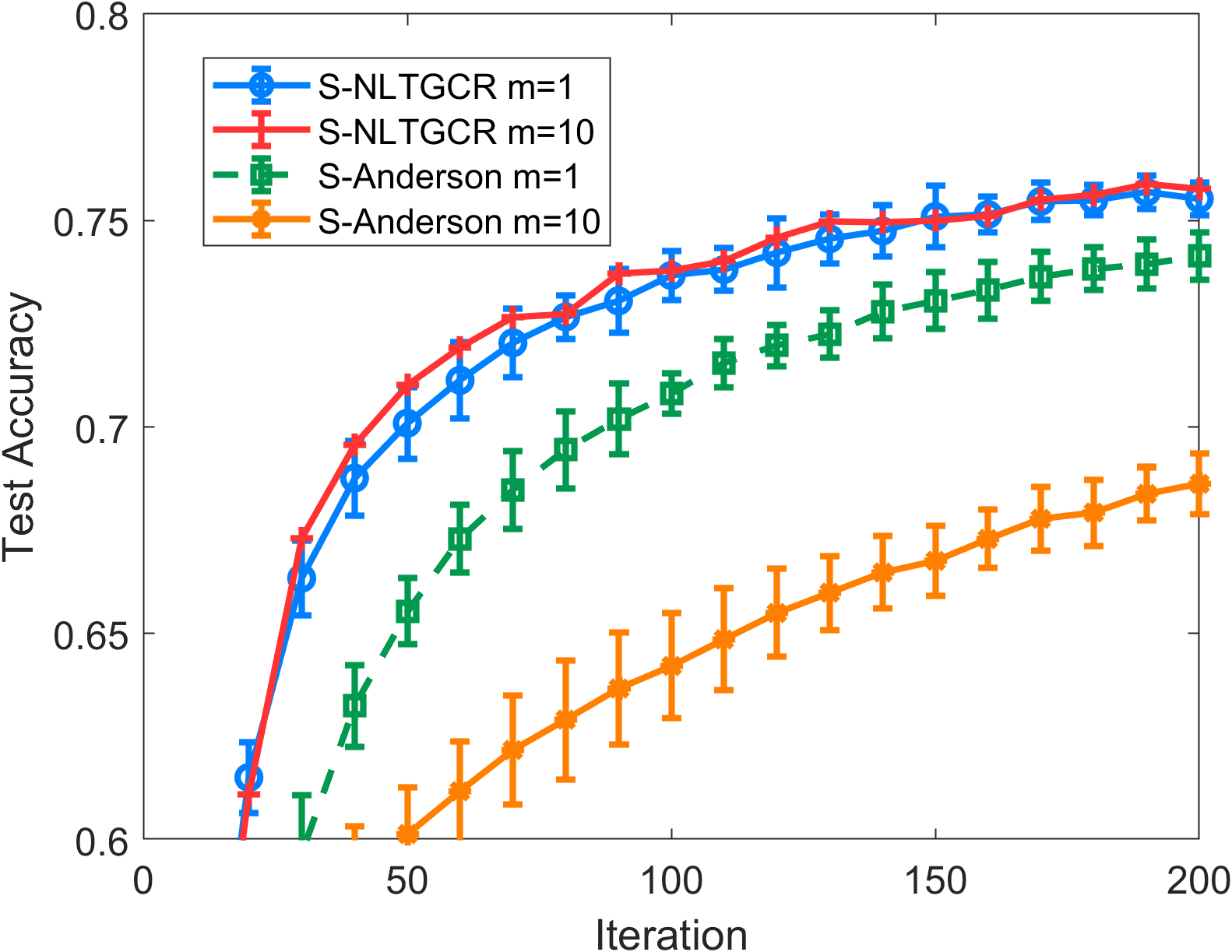
In the main paper, we report the effectiveness of NLTGCR for softmax regression on MNIST. We give the result about using deterministic and stochastic gradients in Figure 2 and find that NLTGCR only requires a small batch size and table size () . In this section, we further investigate the effectiveness of NLTGCR in a stochastic setting, provide additional experimental results in Figure 6 and Figure 7. From Figure 6, we can observe that using the same batch size and table size , stochastic NLTGCR consistently outperforms stochastic AA. Also, it can be observed from Figure 7 that stochastic NLTGCR outperforms stochastic AA for different table size using a fixed batch size of 1500. Although the short-term property does not strictly hold in a stochastic setting, we can still observe that NLTGCR outperforms AA with a smaller variance. In addition, it is worth noting that a smaller table size works better for both NLTGCR and AA. We suspect this is due to the accumulation of inaccurate gradient estimates.
Compatible with Momentum
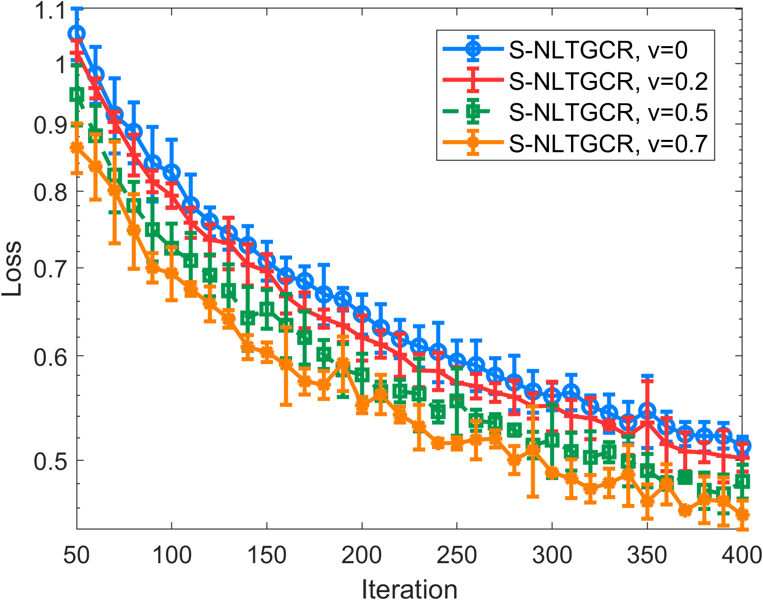
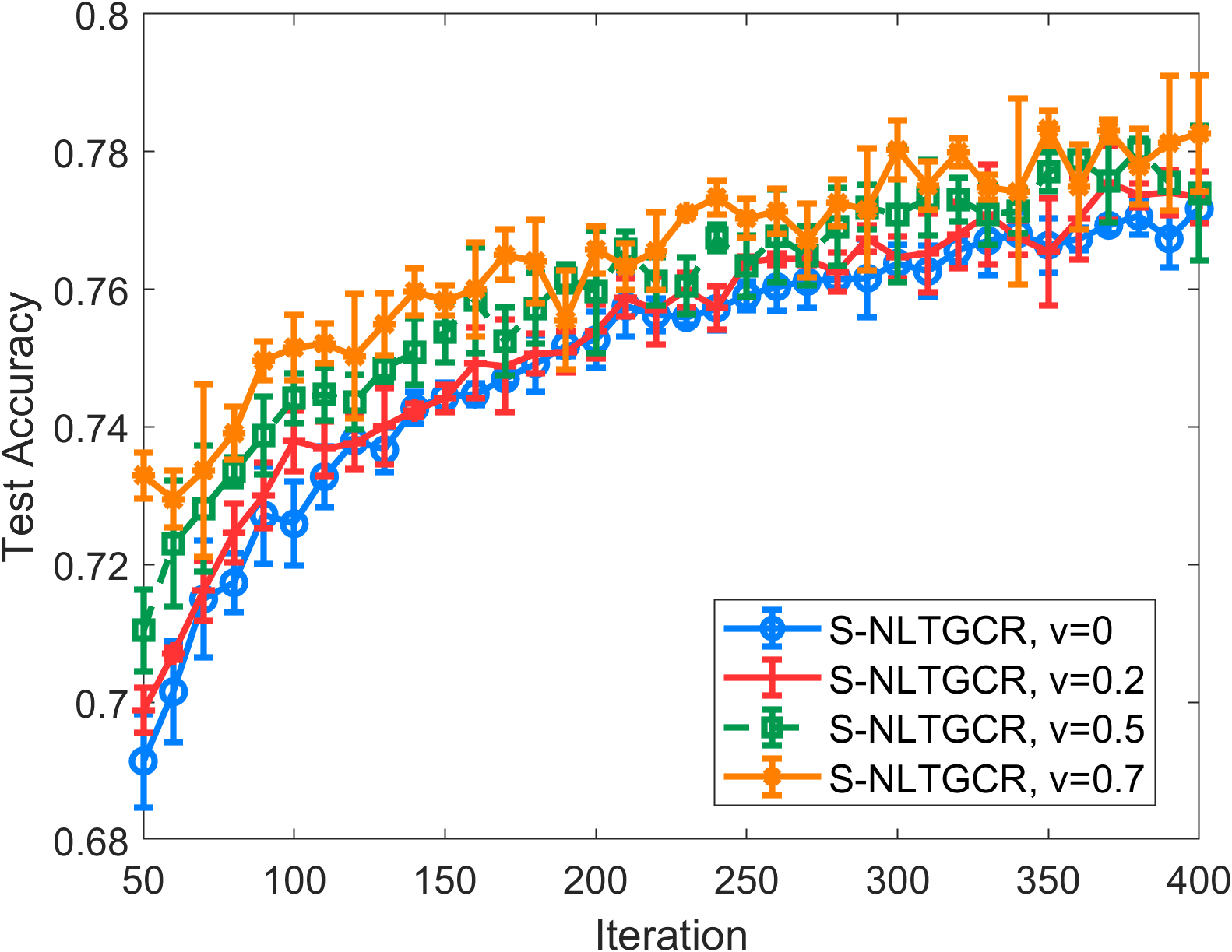
Another important technique in optimization is momentum, which speeds up convergence significantly both in theory and in practice. We experimentally show that it is possible to further accelerate the convergence of NLTGCR by using Momentum. We run stochastic NLTGCR with different momentum term and present results in Figure 8. It suggests that by incorporating momentum into NLTGCR momentum further accelerates the convergence, although the variance gets larger for a large momentum term . We leave the theoretical analysis of of NLTGCR with momentum for future work.
C.5 Results for Deep learning applications
C.5.1 Image classification using CNN
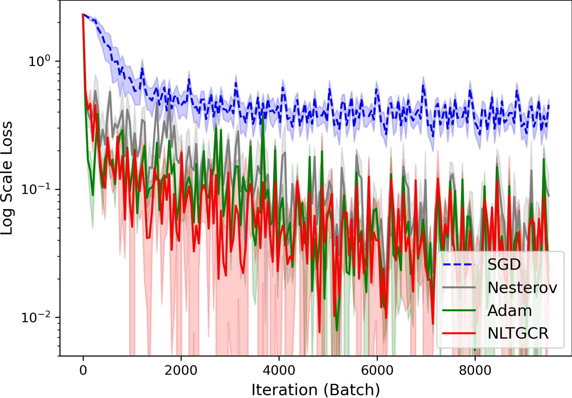
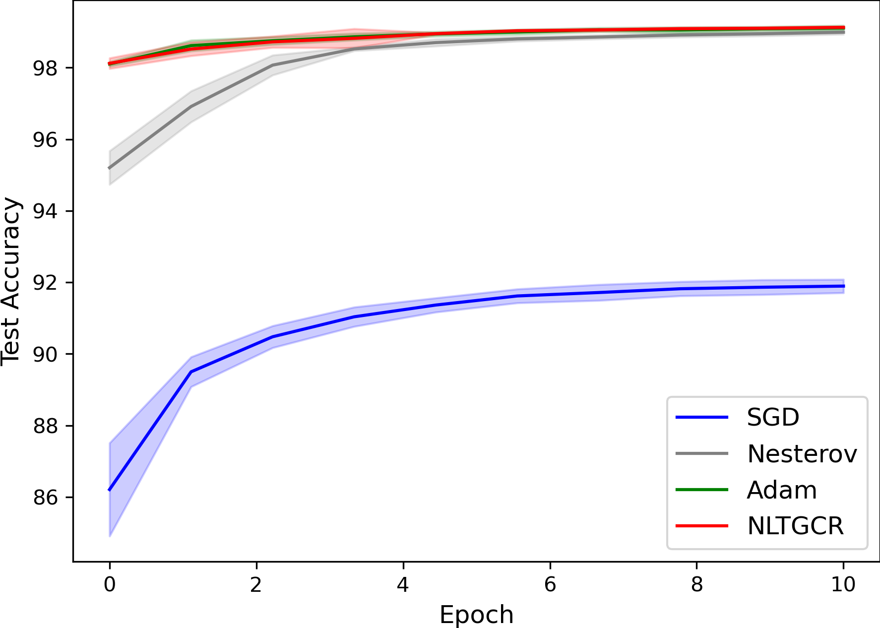
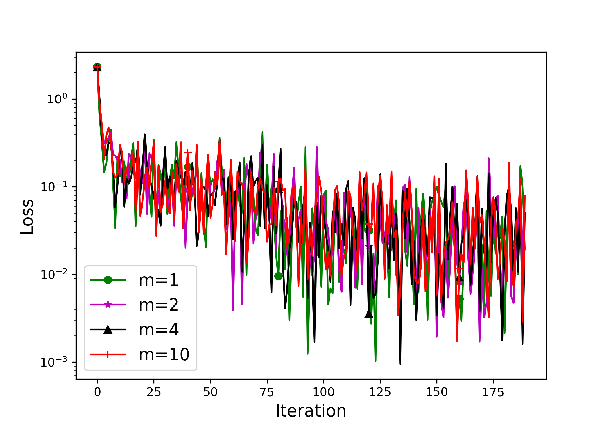
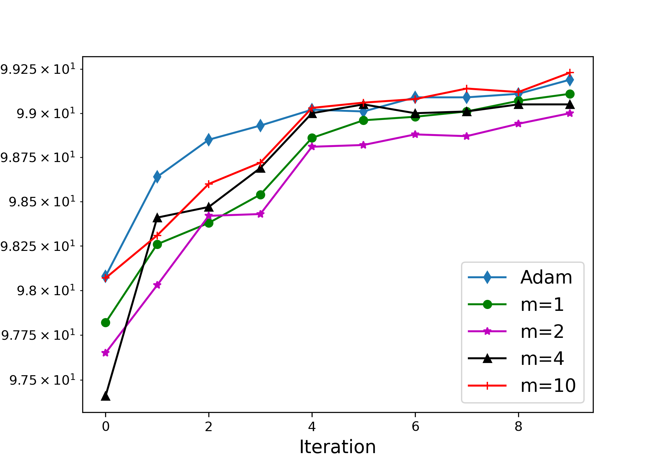
In a more realistic setting, we test our algorithm for neural networks on an image classification task. Particularly, we use the standard MNIST dataset 222http://yann.lecun.com/exdb/mnist/. The architecture of the network is based on the official PyTorch implementation 333implementation https://github.com/pytorch/examples/blob/master/mnist.. We tried our best to ensure that the baselines had the best performance in the tests. Hyperparamters are selected after grid search. We use a batch size of . For SGD, Nestrov (), Adam (default and ), and NLTGCR , we use a learning rate of , , , and , respectively. Figure 9(a) shows the curves of loss for training the neural network on MNIST. Figure 9(b) shows the curves of test accuracy on MNIST. It can be found that NLTGCR outperforms SGD and Nestrov and is comparable to Adam. In addition, we conduct experiments on the effects of table size for NLTGCR and present results in Figure 10. Although Figure 10(b), shows does slightly better, we found that generally yields robust results. In addition, significantly reduces the memory and computation overhead. As a result, we would like to suggest for general experiments. These preliminary results provide insights of the effectiveness of our algorithm for training neural networks. Our algorithm is comparable with the widely used optimizer, Adam. In addition, our algorithm is more memory and computation efficient than other nonlinear acceleration methods including AA and RNA. As a result, it is worth investigating the performance of NLTGCR for different tasks and more complex networks. We leave it for our future work.
C.5.2 Image classification using ResNet
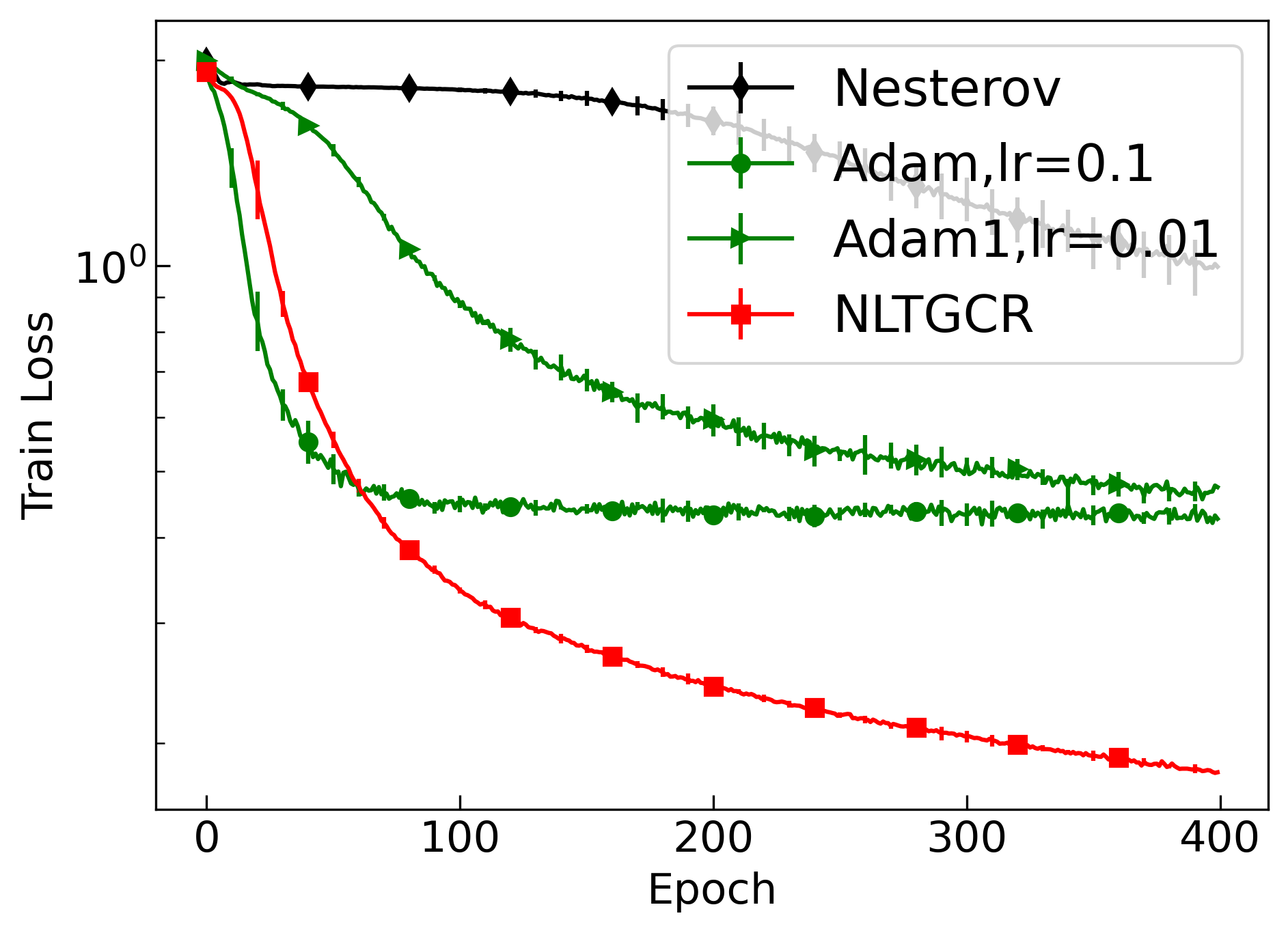
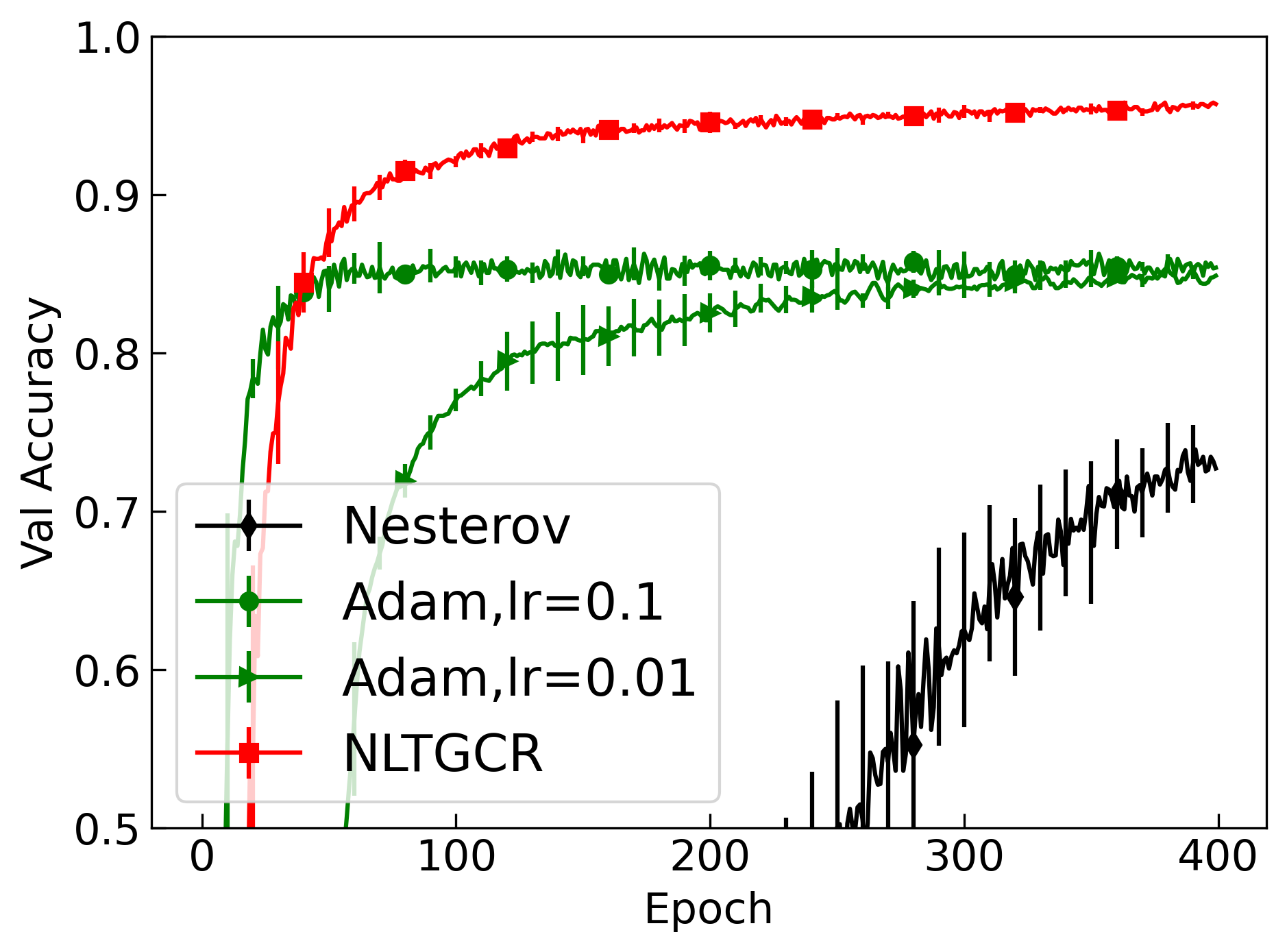
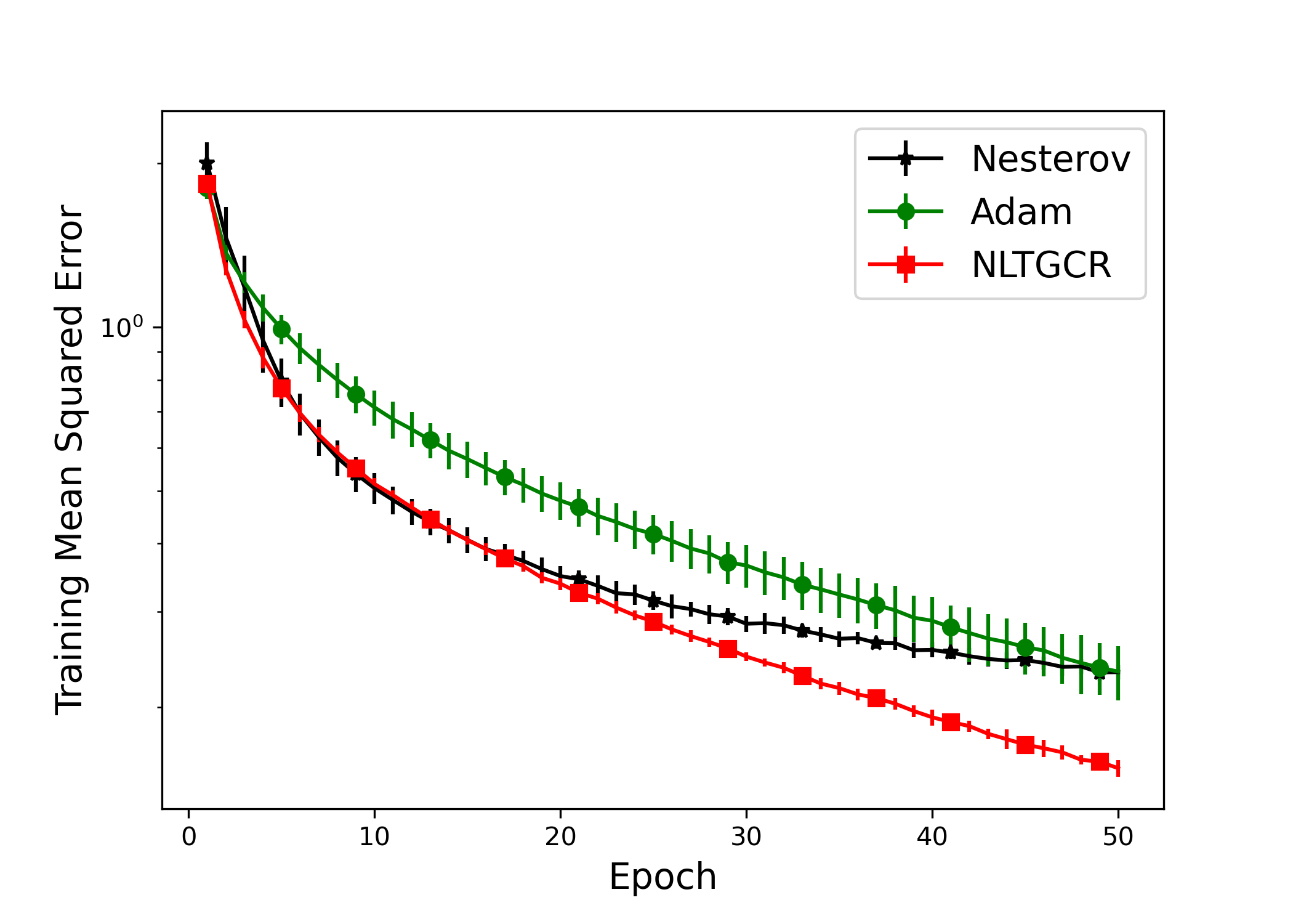
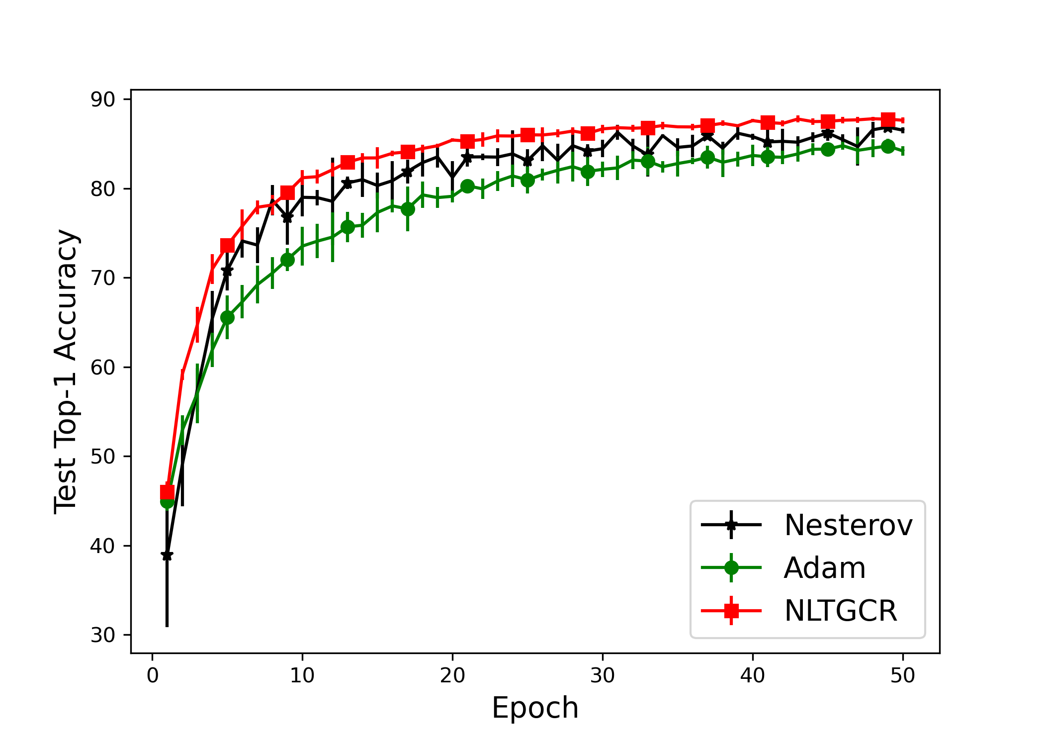
We now perform our tests on ResNet32 [28] 444https://github.com/akamaster/pytorch_resnet_cifar10 using CIFAR10 [37]. We randomly split the training set of all the datasets into two subsets, train and validation. The former is used to train the neural network, whereas the latter is used for measuring the performance of the learned model. Hyperparameters are selected after a grid search. We use a batch size of . For Nesterov (), Adam (default and ), and NLTGCR , we use a learning rate of , , and , respectively. For better visualization, figure 11 shows the curves of training loss and validation accuracy using 50 epochs. It can be observed that nlTGCR(1) consistently outperforms baselines and has a smaller variance.
C.5.3 Time series forecasting using LSTM
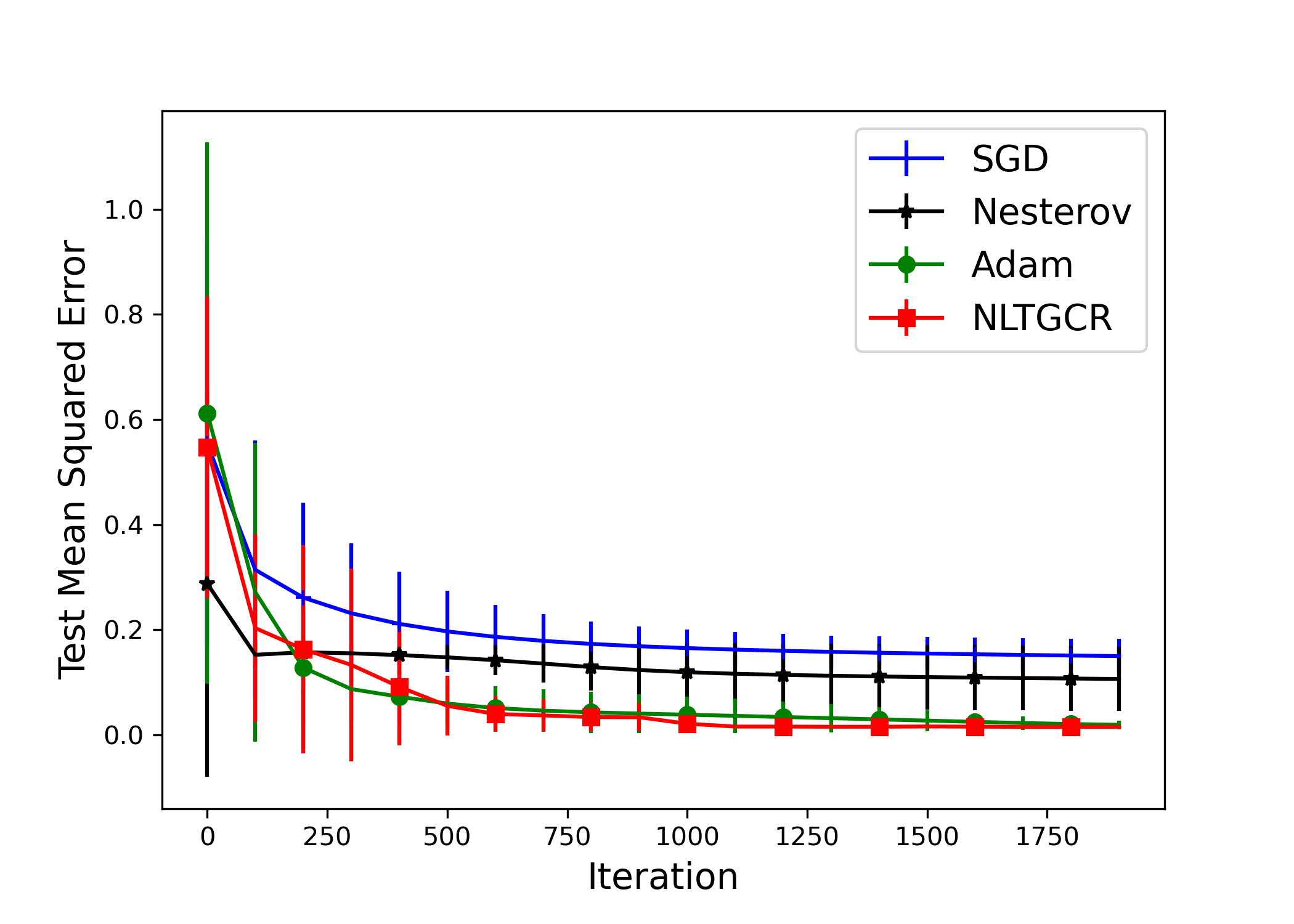
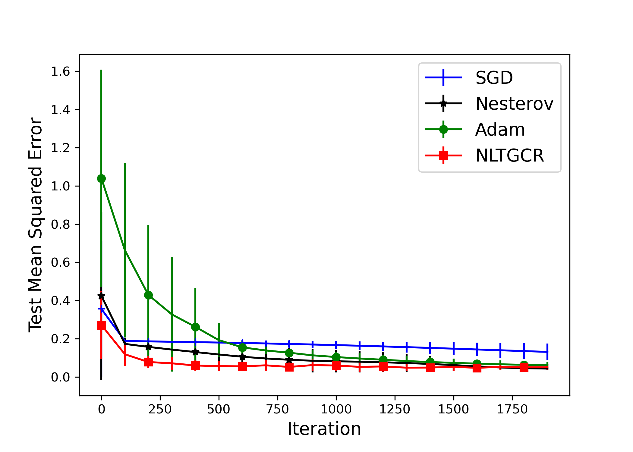
Next, we test our algorithm for Long Short-Term Memory [32] on time series forecasting task using Airplane Passengers and Shampoo Sales Dataset 555https://github.com/spdin/time-series-prediction-lstm-pytorch. We use a learning rate of 0.04 and the mean squared error (MSE) as our loss function and evaluation metric. Figure 12 depicts the MSE on validation set during training. It shows TGCR converges better than baselines. It also suggests TGCR is capable of optimizing complex deep learning architectures.
C.5.4 Semi-supervised classification of graph data using GCN
We also test the effectiveness of nlTGCR on GCN [36] using Cora Dataset. It consists of 2708 scientific publications classified into one of seven different classes. The citation network consists of 5429 links. Each publication in the dataset is described by a 0/1-valued word vector indicating the absence/presence of the corresponding word from the dictionary. The objective is to accurately predict the subject of a paper given its words and citation network, as known as node classification. Hyperparameters are selected after a grid search. For Nesterov (), Adam (default and ), and NLTGCR , we use a learning rate of , , and , respectively. Figure 13(a) and 13(b) depict the training loss and validation accuracy averaged on 5 runs. It shows TGCR converges faster and achieves higher accuracy than baselines, which demonstrates the effectiveness of TGCR optimizing complex deep learning architectures.
