Toda lattice with constraint of type B

We introduce a new integrable hierarchy of nonlinear differential-difference equations which is a subhierarchy of the 2D Toda lattice defined by imposing a constraint to the Lax operators of the latter. The 2D Toda lattice with the constraint can be regarded as a discretization of the BKP hierarchy. We construct its algebraic-geometrical solutions in terms of Riemann and Prym theta-functions.

1 Introduction

The 2D Toda lattice hierarchy [2] plays a very important role in the theory of integrable systems. The commuting flows of the hierarchy are parametrized by infinite sets of complex time variables ${\bf t}=\{t_{1},t_{2},t_{3},\ldots\}$ (“positive times”) and $\bar{\bf t}=\{\bar{t}_{1},\bar{t}_{2},\bar{t}_{3},\ldots\}$ (“negative times”), together with the “zeroth time” $n\in\mbox{\Bbb Z}$. Equations of the hierarchy are differential in the times ${\bf t}$, $\bar{\bf t}$ and difference in $n$. They can be represented in the Lax form as evolution equations for two Lax operators $L$, $\bar{L}$ which are pseudo-difference operators, i.e., half-infinite sums of integer powers of the shift operators $e^{\pm\partial_{n}}$ with coefficients depending on $n$ and ${\bf t}$, $\bar{\bf t}$. A common solution is provided by the tau-function $\tau=\tau(n,{\bf t},\bar{\bf t})$ which satisfies an infinite set of bilinear differential-difference equations of Hirota type [3, 4].

It turns out that it is possible to impose some constraints on the Lax operators in such a way that they would be consistent with the dynamics of the Toda hierarchy. One of such examples was considered in our previous work [5], where we have introduced the Toda hierarchy with a constraint of type C, which is $\bar{L}=L^{{\dagger}}$ (in the symmetric gauge). Here and below $L^{{\dagger}}$ is the conjugate operator ($(f(n)\circ e^{\partial_{n}})^{{\dagger}}=e^{-\partial_{n}}\circ f(n)$). It is a subhierarchy of the Toda lattice which can be regarded as an integrable discretization of the CKP hierarchy [6]-[11].

The purpose of this paper is to elaborate another example and to introduce a new integrable hierarchy: the Toda hierarchy with the constraint of type B. In a special gauge, which we call the balanced gauge, it reads:

$$L^{{\dagger}}=(e^{\partial_{n}}-e^{-\partial_{n}})\bar{L}(e^{\partial_{n}}-e^{-\partial_{n}})^{-1}.$$ (1.1)

This constraint is preserved by the flows $\partial_{t_{k}}-\partial_{\bar{t}_{k}}$ and is destroyed by the flows $\partial_{t_{k}}+\partial_{\bar{t}_{k}}$, so to define the hierarchy one should restrict the times as $\bar{t}_{k}=-t_{k}$. This hierarchy is an integrable discretization of the BKP hierarchy [6, 7, 12, 13, 14, 15, 16] which is defined by imposing the constraint

$$(L^{\rm KP})^{{\dagger}}=-\partial_{x}L^{\rm KP}\partial_{x}^{-1},\qquad x=t_{1}$$ (1.2)

on the pseudo-differential Lax operator of the KP hierarchy, that is why we call (1.1), looking as a difference analogue of (1.2), “the constraint of type B”. The first member of the hierarchy is the following system of equations for two unknown functions $v$, $f_{0}$:

$$\left\{\begin{array}[]{l}\displaystyle{\partial_{t_{1}}\log\Bigl{(}v(n)v(n+1)\Bigr{)}=\frac{f_{0}(n+1)}{v(n+1)}}-\frac{f_{0}(n)}{v(n)},\\ \\ \partial_{t_{2}}v(n)-\partial_{t_{1}}f_{0}(n)=2v^{2}(n)\Bigl{(}v(n-1)-v(n+1)\Bigr{)}.\end{array}\right.$$ (1.3)

Let us note that essentially the same hierarchy was suggested in the paper [17] as an integrable discretization of the Novikov-Veselov equation. However, the close connection with the Toda lattice was not mentioned there.

We construct algebraic-geometrical (quasi-periodic) solutions of the Toda lattice with the constraint of type B. These solutions are built from algebraic curves with holomorphic involution $\iota$ having exactly two fixed points $Q_{1},Q_{2}$ (ramified coverings with two branch points) and two marked points $P_{0}$, $P_{\infty}$ such that $\iota(P_{0})=P_{\infty}$. We show that the solutions can be expressed in terms of Prym theta-functions. A similar but different construction was given in [17], where unramified coverings with two pairs of marked points were considered.

Solutions to the Toda lattice with the constraint of type B can be expressed in terms of the tau-function $\tau^{B}(n)=\tau^{B}(n,{\bf t})$ as follows:

$$v(n)=\frac{\tau^{B}(n+1)\tau^{B}(n-1)}{(\tau^{B}(n))^{2}},\quad f_{0}(n)=v(n)\,\partial_{t_{1}}\!\log\frac{\tau^{B}(n+1)}{\tau^{B}(n-1)}.$$ (1.4)

The tau-function $\tau^{B}(n)$ of the Toda lattice with the constraint is related to the tau-function $\tau(n)$ of the Toda lattice as

$$\tau(n)=\tau^{B}(n)\tau^{B}(n-1).$$ (1.5)

This relation should be compared with the relation between tau-functions of the KP and BKP hierarchies: the former is the square of the latter. In the Toda case, it is not the square but the arguments of the two factors are shifted by $1$; in the continuum limit they become the same.

We show that for algebraic-geometrical solutions of equations (1.3), constructed starting from a smooth algebraic curve $\Gamma$ with holomorphic involution (having exactly two fixed points) and a divisor satisfying some special condition (see (3.4) below), the tau-function $\tau^{B}(n)$ is expressed in terms of Prym theta-function $\Theta_{\rm Pr}$:

$$\tau^{B}(n,{\bf t})=e^{-L(n,{\bf t})-\frac{1}{2}\,Q(n,{\bf t})}\,\Theta_{\rm Pr}\Bigl{(}n\vec{u}_{0}+\sum_{k\geq 1}\vec{u}_{k}t_{k}+\vec{z}\Bigr{)},$$ (1.6)

where $L(n,{\bf t})$, $Q(n,{\bf t})$ are linear and quadratic forms in $n$, ${\bf t}$ respectively and $\vec{u}_{i}$ are periods of certain differentials on the algebraic curve $\Gamma$.

To avoid a confusion, we should stress that our Toda hierarchies with constraints of types C and B introduced in [5] and in this paper respectively, are very different from what is called C- and B-Toda in [2].

In section 2, after a short reminder about the general Toda lattice, we introduce the constraint of type B and prove that it is consistent with the hierarchy if one restricts the time variables to the submanifold $t_{k}+\bar{t}_{k}=0$ in the space of independent variables. The first nontrivial equations of the hierarchy are obtained in the explicit form. Section 3 is devoted to the construction of algebraic-geometrical solutions in terms of Prym theta-functions. The main technical tool is the Baker-Akhiezer function. All necessary facts about algebraic curves, differentials and theta-functions are given in the appendix.

2 The Toda hierarchy of type B

2.1 2D Toda lattice

First of all, we briefly review the 2D Toda lattice hierarchy following [2]. Let us consider the pseudo-difference Lax operators

$${\cal L}=e^{\partial_{n}}+\sum_{k\geq 0}U_{k}(n)e^{-k\partial_{n}},\quad\bar{\cal L}=c(n)e^{-\partial_{n}}+\sum_{k\geq 0}\bar{U}_{k}(n)e^{k\partial_{n}},$$ (2.1)

where $e^{\partial_{n}}$ is the shift operator acting as $e^{\pm\partial_{n}}f(x)=f(n\pm 1)$. The coefficient functions $c(n)$, $U_{k}(n)$, $\bar{U}_{k}(n)$ are functions of $n$ and all the times ${\bf t}$, $\bar{\bf t}$. The Lax equations are

$$\begin{array}[]{l}\partial_{t_{m}}{\cal L}=[{\cal B}_{m}+\Phi_{m},{\cal L}],\quad\partial_{t_{m}}\bar{\cal L}=[{\cal B}_{m}+\Phi_{m},\bar{\cal L}],\quad{\cal B}_{m}=({\cal L}^{m})_{>0},\quad\Phi_{m}=({\cal L}^{m})_{0},\\ \\ \partial_{\bar{t}_{m}}{\cal L}=[\bar{\cal B}_{m},{\cal L}],\quad\partial_{\bar{t}_{m}}\bar{\cal L}=[\bar{\cal B}_{m},\bar{\cal L}],\quad\bar{\cal B}_{m}=(\bar{\cal L}^{m})_{<0}.\end{array}$$ (2.2)

Here and below, given a subset $\mbox{\Bbb S}\subset\mbox{\Bbb Z}$, we denote $\displaystyle{\Bigl{(}\sum_{k\in\raise-1.0pt\hbox{$\mbox{\Bbbb Z}$}}U_{k}e^{k\eta\partial_{x}}\Bigr{)}_{\raise-1.0pt\hbox{$\mbox{\Bbbb S}$}}=\sum_{k\in\raise-1.0pt\hbox{$\mbox{\Bbbb S}$}}U_{k}e^{k\eta\partial_{x}}}$. For example,

$$\begin{array}[]{l}{\cal B}_{1}=e^{\partial_{n}},\qquad\bar{\cal B}_{1}=c(n)e^{-\partial_{n}},\\ \\ {\cal B}_{2}=e^{2\partial_{n}}+(U_{0}(n)+U_{0}(n+1))e^{\partial_{n}},\\ \\ \bar{\cal B}_{2}=c(n)c(n-1)e^{-2\partial_{n}}+c(n)(\bar{U}_{0}(n)+\bar{U}_{0}(n-1))e^{-\partial_{n}},\\ \\ \Phi_{1}=U_{0}(n),\qquad\Phi_{2}=U_{1}(n)+U_{1}(n+1)+U_{0}^{2}(n).\end{array}$$ (2.3)

We will also use the notation $(\ldots)_{+}=(\ldots)_{>0}$, $(\ldots)_{-}=(\ldots)_{<0}$. Setting

$$c(n)=e^{\varphi(n)-\varphi(n-1)},$$ (2.4)

we have from (2.2):

$$\partial_{t_{m}}\varphi=\Phi_{m},\quad\partial_{\bar{t}_{m}}\varphi=-(\bar{\cal L}^{m})_{0}:=-\bar{\Phi}_{m}.$$ (2.5)

In terms of the function $\varphi(n)$ the first equation of the Toda lattice hierarchy has the form

$$\partial_{t_{1}}\partial_{\bar{t}_{1}}\varphi(n)=e^{\varphi(n)-\varphi(n-1)}-e^{\varphi(n+1)-\varphi(n)}.$$ (2.6)

The common solution of the hierarchy is given by the tau-function $\tau(n)=\tau(n,{\bf t},\bar{\bf t})$. In particular,

$$e^{\varphi(n)}=\frac{\tau(n+1)}{\tau(n)}.$$ (2.7)

There exist other equivalent formulations of the Toda hierarchy obtained from the one given above by gauge transformations [18, 19]. So far we have used the standard gauge in which the coefficient of the first term of ${\cal L}$ is fixed to be $1$. In fact there is a family of gauge transformations with a function $g=g(n)$ of the form

$${\cal L}\to g^{-1}{\cal L}g,\quad\bar{\cal L}\to g^{-1}\bar{\cal L}g,$$

$${\cal B}_{n}\to g^{-1}{\cal B}_{n}g-g^{-1}\partial_{t_{n}}g,\quad\bar{\cal B}_{n}\to g^{-1}\bar{\cal B}_{n}g-g^{-1}\partial_{\bar{t}_{n}}g.$$

We are interested in another special gauge in which the coefficients in front of the first terms of the two Lax operators coincide. Let us denote the Lax operators and the generators of the flows in this gauge by $L$, $\bar{L}$, $B_{m}$, $\bar{B}_{m}$ respectively:

$$\begin{array}[]{c}L=g^{-1}{\cal L}g,\quad\bar{L}=g^{-1}\bar{\cal L}g,\\ \\ B_{m}=g^{-1}{\cal B}_{m}g+\Phi_{m}-\partial_{t_{m}}\log g,\quad\bar{B}_{m}=g^{-1}\bar{\cal B}_{m}g-\partial_{\bar{t}_{m}}\log g.\end{array}$$ (2.8)

It is easy to see that the function $g(n)$ is determined from the relation

$$e^{\varphi(n)}=g(n)g(n+1).$$ (2.9)

We call this gauge the balanced gauge.

An equivalent formulation of the Toda hierarchy is through the Zakharov-Shabat equations

$$\begin{array}[]{l}\partial_{t_{n}}B_{m}-\partial_{t_{m}}B_{n}+[B_{m},B_{n}]=0,\\ \\ \partial_{\bar{t}_{n}}B_{m}-\partial_{t_{m}}\bar{B}_{n}+[B_{m},\bar{B}_{n}]=0,\\ \\ \partial_{\bar{t}_{n}}\bar{B}_{m}-\partial_{\bar{t}_{m}}\bar{B}_{n}+[\bar{B}_{m},\bar{B}_{n}]=0.\end{array}$$ (2.10)

They are compatibility conditions for the auxiliary linear problems

$$\partial_{t_{m}}\Psi=B_{m}\Psi,\quad\partial_{\bar{t}_{m}}\Psi=\bar{B}_{m}\Psi.$$ (2.11)

The wave function $\Psi=\Psi(n,{\bf t},\bar{\bf t},k)$ depends on a spectral parameter $k\in\mbox{\Bbb C}$. We will often skip the dependence on ${\bf t}$, $\bar{\bf t}$ writing simply $\Psi=\Psi(n,k)$. The wave function has the following expansions as $k\to\infty$ and $k\to 0$:

$$\Psi(n,k)=\left\{\begin{array}[]{l}\displaystyle{k^{n}e^{\xi({\bf t},k)}e^{\varphi_{+}(n)}\Bigl{(}1+\sum_{s\geq 1}\xi_{s}(n)k^{-s}\Bigr{)},\quad k\to\infty,}\\ \\ \displaystyle{k^{n}e^{\xi(\bar{\bf t},k^{-1})}e^{\varphi_{-}(n)}\Bigl{(}1+\sum_{s\geq 1}\chi_{s}(n)k^{s}\Bigr{)},\quad k\to 0,}\end{array}\right.$$ (2.12)

where $\displaystyle{\xi({\bf t},k)=\sum_{j\geq 1}t_{j}k^{j}}$.

It is convenient to represent the wave function as a result of acting of the dressing operators $W$, $\bar{W}$ to the exponential function

$$E(n,{\bf t},k)=k^{n}e^{\xi({\bf t},k)}.$$

The dressing operators are pseudo-difference operators of the form

$$\begin{array}[]{l}\displaystyle{W=e^{\varphi_{+}(n)}\Bigl{(}1+\sum_{s\geq 1}\xi_{s}(n)e^{-s\partial_{n}}\Bigr{)},}\\ \\ \displaystyle{\bar{W}=e^{\varphi_{-}(n)}\Bigl{(}1+\sum_{s\geq 1}\chi_{s}(n)e^{s\partial_{n}}\Bigr{)},}\end{array}$$ (2.13)

so that

$$\Psi(n,k)=\left\{\begin{array}[]{l}\displaystyle{WE(n,{\bf t},k),\quad k\to\infty},\\ \\ \displaystyle{\bar{W}E(-n,\bar{\bf t},k^{-1}),\quad k\to 0.}\end{array}\right.$$ (2.14)

The Lax operators are obtained by “dressing” of the shift operators as follows:

$$L=We^{\partial_{n}}W^{-1},\quad\bar{L}=\bar{W}e^{-\partial_{n}}\bar{W}^{-1}.$$ (2.15)

It is clear from (2.15) that the wave function is an eigenfunction of the operators $L$, $\bar{L}$:

$$L\Psi(n,k)=k\Psi(n,k),\quad\bar{L}\Psi(n,k)=k^{-1}\Psi(n,k).$$ (2.16)

Let us introduce the dual wave function $\Psi^{*}$ as

$$\Psi^{*}(n,k)=(W^{{\dagger}})^{-1}E^{-1}(n,{\bf t},k),\quad k\to\infty,$$ (2.17)

where conjugation of difference operators (the ${\dagger}$-operation) is defined on shift operators as

$$(f(n)\circ e^{\partial_{n}})^{{\dagger}}=e^{-\partial_{n}}\circ f(n)$$

and is extended to all difference and pseudo-difference operators by linearity. The following lemmas are well-known.

Lemma 2.1

The dual wave function satisfies the conjugate linear equations

$$\begin{array}[]{c}L^{{\dagger}}\Psi^{*}(n,k)=k\Psi^{*}(n,k),\\ \\ -\partial_{t_{m}}\Psi^{*}(n,k)=B_{m}^{{\dagger}}\Psi^{*}(n,k),\quad-\partial_{\bar{t}_{m}}\Psi^{*}(n,k)=\bar{B}_{m}^{{\dagger}}\Psi^{*}(n,k).\end{array}$$ (2.18)

Lemma 2.2

The wave function and its dual satisfy the bilinear relation

$$\oint_{C_{\infty}}\Psi(n,{\bf t},\bar{\bf t},k)\Psi^{*}(n^{\prime},{\bf t}^{\prime},\bar{\bf t}^{\prime},k)\frac{dk}{k}=\oint_{C_{0}}\Psi(n,{\bf t},\bar{\bf t},k)\Psi^{*}(n^{\prime},{\bf t}^{\prime},\bar{\bf t}^{\prime},k)\frac{dk}{k}$$ (2.19)

for all $n,n^{\prime}$, ${\bf t},\,{\bf t}^{\prime}$, $\bar{\bf t},\,\bar{\bf t}^{\prime}$, where $C_{\infty}$, $C_{0}$ are small contours around $\infty$, $0$ respectively.

2.2 The constraint of type B

Let us define the operator

$$T=e^{-\varphi(n)}e^{\partial_{n}}$$ (2.20)

and consider the following constraint on the two Lax operators in the standard gauge:

$$(T-T^{{\dagger}})\bar{\cal L}={\cal L}^{{\dagger}}(T-T^{{\dagger}}).$$ (2.21)

As is easy to see, in the balanced gauge this constraint acquires the form

$$(e^{\partial_{n}}-e^{-\partial_{n}})\bar{L}=L^{{\dagger}}(e^{\partial_{n}}-e^{-\partial_{n}}).$$ (2.22)

Theorem 2.1

The constraint (2.21) is invariant under the flows $\partial_{t_{k}}\!-\!\partial_{\bar{t}_{k}}$ for all $k\geq 1$.

Proof. We should prove that

$$(\partial_{t_{k}}\!-\!\partial_{\bar{t}_{k}})\Bigl{[}(T-T^{{\dagger}})\bar{\cal L}-{\cal L}^{{\dagger}}(T-T^{{\dagger}})\Bigr{]}=0.$$

Basically, this is a straightforward calculation which uses the Lax equations and the equations $\partial_{t_{k}}T=-\Phi_{k}T$, $\partial_{\bar{t}_{k}}T=\bar{\Phi}_{k}T$. Here are some details. Denoting

$${\cal A}_{k}={\cal B}_{k}-\bar{\cal B}_{k},$$

we can write, after some cancellations:

$$\begin{array}[]{c}(\partial_{t_{k}}\!-\!\partial_{\bar{t}_{k}})\Bigl{[}(T-T^{{\dagger}})\bar{\cal L}-{\cal L}^{{\dagger}}(T-T^{{\dagger}})\Bigr{]}\\ \\ =\Bigl{(}(T\!-\!T^{{\dagger}}){\cal A}_{k}+{\cal A}_{k}^{{\dagger}}(T\!-\!T^{{\dagger}})\Bigr{)}\bar{\cal L}-{\cal L}^{{\dagger}}\Bigl{(}(T\!-\!T^{{\dagger}}){\cal A}_{k}+{\cal A}_{k}^{{\dagger}}(T\!-\!T^{{\dagger}})\Bigr{)}\\ \\ -\Phi_{k}T\bar{\cal L}-\bar{\Phi}_{k}T\bar{\cal L}+T^{{\dagger}}\bar{\Phi}_{k}\bar{\cal L}+{\cal L}^{{\dagger}}\bar{\Phi}_{k}T-{\cal L}^{{\dagger}}T^{{\dagger}}\bar{\Phi}_{k}-{\cal L}^{{\dagger}}T^{{\dagger}}\Phi_{k}+T\Phi_{k}\bar{\cal L}-T\bar{\cal L}\Phi_{k}\\ \\ +T^{{\dagger}}\bar{\cal L}\Phi_{k}+\Phi_{k}{\cal L}^{{\dagger}}T-\Phi_{k}{\cal L}^{{\dagger}}T^{{\dagger}}+{\cal L}^{{\dagger}}\Phi_{k}T^{{\dagger}}.\end{array}$$ (2.23)

Now, writing

$$(T-T^{{\dagger}})\bar{\cal L}^{k}-({\cal L}^{{\dagger}})^{k}(T-T^{{\dagger}})=0$$

and taking the $(\ldots)_{-}$-part of this equality, we get

$$(T-T^{{\dagger}})\bar{\cal B}_{k}-{\cal B}_{k}^{{\dagger}}(T-T^{{\dagger}})=-(({\cal L}^{{\dagger}})^{k})_{-1}e^{-\partial_{n}}T+T(\bar{\cal L}^{k})_{-1}e^{-\partial_{n}}-\Phi_{k}T^{{\dagger}}+T^{{\dagger}}\bar{\Phi}_{k}.$$ (2.24)

Similarly, writing

$$(T-T^{{\dagger}}){\cal L}^{k}-(\bar{\cal L}^{{\dagger}})^{k}(T-T^{{\dagger}})=0$$

and taking the $(\ldots)_{+}$-part of this equality, we get

$$(T-T^{{\dagger}}){\cal B}_{k}-\bar{\cal B}_{k}^{{\dagger}}(T-T^{{\dagger}})=((\bar{\cal L}^{{\dagger}})^{k})_{1}e^{\partial_{n}}T^{{\dagger}}-T^{{\dagger}}({\cal L}^{k})_{1}e^{\partial_{n}}+\bar{\Phi}_{k}T-T\Phi_{k}.$$ (2.25)

Subtracting (2.24) from (2.25) and taking into account that

$$T(\bar{\cal L}^{k})_{-1}e^{-\partial_{n}}=((\bar{\cal L}^{{\dagger}})^{k})_{1}e^{\partial_{n}}T^{{\dagger}},\quad(({\cal L}^{{\dagger}})^{k})_{-1}e^{-\partial_{n}}T=T^{{\dagger}}({\cal L}^{k})_{1}e^{\partial_{n}},$$

we obtain:

$$(T\!-\!T^{{\dagger}}){\cal A}_{k}+{\cal A}_{k}^{{\dagger}}(T\!-\!T^{{\dagger}})=\bar{\Phi}_{k}T-T\Phi_{k}+\Phi_{k}T^{{\dagger}}-T^{{\dagger}}\bar{\Phi}_{k}.$$

Plugging this into (2.23) we see that all terms in the right hand side cancel and we get zero.  

We have proved that the constraint (2.21) remains intact under the flows $\partial_{t_{k}}\!-\!\partial_{\bar{t}_{k}}$. However, it is destroyed by the flows $\partial_{t_{k}}\!+\!\partial_{\bar{t}_{k}}$.

The invariance of the constraint proved in the standard gauge implies that the constraint in the balanced gauge is invariant, too, i.e.

$$(\partial_{t_{k}}-\partial_{\bar{t}_{k}})\Bigl{[}(e^{\partial_{n}}-e^{-\partial_{n}})\bar{L}-L^{{\dagger}}(e^{\partial_{n}}-e^{-\partial_{n}})\Bigr{]}=0.$$ (2.26)

In the balanced gauge, the generators of the flows $\partial_{t_{k}}-\partial_{\bar{t}_{k}}$ are

$$A_{k}=B_{k}-\bar{B}_{k}.$$ (2.27)

A straightforward calculation which uses the Lax equations allows one to prove that (2.26) implies

$$(e^{\partial_{n}}-e^{-\partial_{n}})A_{k}+A_{k}^{{\dagger}}(e^{\partial_{n}}-e^{-\partial_{n}})=0$$ (2.28)

or

$$A_{k}^{{\dagger}}=-(e^{\partial_{n}}-e^{-\partial_{n}})A_{k}(e^{\partial_{n}}-e^{-\partial_{n}})^{-1}.$$ (2.29)

As soon as $A_{k}^{{\dagger}}$ is a difference operator (a linear combination of a finite number of shifts), this relation suggests that the operator $A_{k}$ must be divisible by $e^{\partial_{n}}-e^{-\partial_{n}}$ from the right:

$$A_{k}=C_{k}(e^{\partial_{n}}-e^{-\partial_{n}}),$$ (2.30)

where $C_{k}$ is a difference operator. The substitution into (2.28) then shows that $C_{k}$ is a self-adjoint operator: $C_{k}=C_{k}^{{\dagger}}$.

2.3 Equations of the Toda lattice of type B

Let us introduce the following linear combinations of times:

$$T_{j}=\frac{1}{2}(t_{j}-\bar{t}_{j}),\quad y_{j}=\frac{1}{2}(t_{j}+\bar{t}_{j}),$$ (2.31)

then the corresponding vector fields are

$$\partial_{T_{j}}=\partial_{t_{j}}-\partial_{\bar{t}_{j}},\quad\partial_{y_{j}}=\partial_{t_{j}}+\partial_{\bar{t}_{j}}.$$ (2.32)

We have seen that the $T_{j}$-flows preserve the constraint while the $y_{j}$-flows destroy it. This suggests to put $y_{j}=0$ for all $j$ and consider the evolution with respect to $T_{j}$ only. In this way one can introduce the Toda hierarchy of type B. The balanced gauge is most convenient for this purpose. According to (2.30), the generators of the $T_{k}$-flows in this gauge have the general form

$$A_{k}=\Bigl{(}f_{0k}+\sum_{j=1}^{k-1}(f_{jk}e^{j\partial_{n}}+e^{-j\partial_{n}}f_{jk})\Bigr{)}(e^{\partial_{n}}-e^{-\partial_{n}}),$$ (2.33)

where $f_{jk}$ are some functions of $n$ and the times $\{T_{i}\}$. The equations of the hierarchy are obtained from the Zakharov-Shabat conditions

$$[\partial_{T_{k}}-A_{k},\,\partial_{T_{m}}-A_{m}]=0$$

or

$$\partial_{T_{m}}A_{k}-\partial_{T_{k}}A_{m}+[A_{k},A_{m}]=0.$$ (2.34)

The simplest equations are obtained when $k=1$, $m=2$. In this case the operators are

$$\begin{array}[]{l}A_{1}=v(n)(e^{\partial_{n}}-e^{-\partial_{n}}),\\ \\ A_{2}=\Bigl{(}f_{0}(n)+f_{1}(n)e^{\partial_{n}}+e^{-\partial_{n}}f_{1}(n)\Bigr{)}(e^{\partial_{n}}-e^{-\partial_{n}}).\end{array}$$ (2.35)

Plugging these into the Zakharov-Shabat equation

$$\partial_{T_{2}}A_{1}-\partial_{T_{1}}A_{2}+[A_{1},A_{2}]=0,$$

we obtain the following system of three equations for three unknown functions:

$$\left\{\begin{array}[]{l}v(n)f_{1}(n+1)=v(n+2)f_{1}(n),\\ \\ \partial_{T_{1}}f_{1}(n)+v(n+1)f_{0}(n)-v(n)f_{0}(n+1)=0,\\ \\ \partial_{T_{2}}v(n)-\partial_{T_{1}}f_{0}(n)+2v(n)\Bigl{(}f_{1}(n)-f_{1}(n-1)\Bigr{)}=0.\end{array}\right.$$ (2.36)

The first equation allows one to exclude the function $f_{1}$:

$$f_{1}(n)=v(n)v(n+1),$$

and the system becomes

$$\left\{\begin{array}[]{l}\displaystyle{\partial_{T_{1}}\log\Bigl{(}v(n)v(n+1)\Bigr{)}=\frac{f_{0}(n+1)}{v(n+1)}-\frac{f_{0}(n)}{v(n)}},\\ \\ \partial_{T_{2}}v(n)-\partial_{T_{1}}f_{0}(n)+2v^{2}(n)\Bigl{(}v(n+1)-v(n-1)\Bigr{)}=0.\end{array}\right.$$ (2.37)

Let us compare the balanced gauge with the standard gauge explicitly. Using equations (2.3) and (2.8), we can write:

$$A_{1}=\frac{g(n+1)}{g(n)}\,e^{\partial_{n}}+U_{0}(n)-\partial_{T_{1}}\log g(n)-\frac{g(n-1)}{g(n)}\,e^{\varphi(n)-\varphi(n-1)}e^{-\partial_{n}},$$ (2.38)

$$\begin{array}[]{c}\displaystyle{A_{2}=\frac{g(n+2)}{g(n)}\,e^{2\partial_{n}}+\frac{g(n+1)}{g(n)}(U_{0}(n)+U_{0}(n+1))e^{\partial_{n}}}\\ \\ \displaystyle{+U_{1}(n)+U_{1}(n+1)+U_{0}^{2}(n)-\partial_{T_{2}}\log g(n)}\\ \\ \displaystyle{-\frac{g(n-1)}{g(n)}\,e^{\varphi(n)-\varphi(n-1)}(U_{0}(n)+U_{0}(n+1))e^{-\partial_{n}}-\frac{g(n-2)}{g(n)}\,e^{\varphi(n)-\varphi(n-2)}e^{-2\partial_{n}}},\end{array}$$ (2.39)

where we have put $\bar{U}_{0}(n)=U_{0}(n+1)$, as it follows from the constraint. Comparing with (2.35), we identify

$$v(n)=\frac{g(n+1)}{g(n)},$$ (2.40)

$$f_{0}(n)=\frac{g(n+1)}{g(n)}\,(U_{0}(n)+U_{0}(n+1))$$ (2.41)

and

$$\partial_{T_{1}}\log g(n)=U_{0}(n).$$ (2.42)

The tau-function of the Toda lattice with the constraint, $\tau^{B}(n)=\tau^{B}(n,{\bf T})$, can be introduced via the relation

$$g(n)=\frac{\tau^{B}(n)}{\tau^{B}(n-1)},$$ (2.43)

then

$$v(n)=\frac{\tau^{B}(n+1)\tau^{B}(n-1)}{(\tau^{B}(n))^{2}},\quad f_{0}(n)=v(n)\,\partial_{T_{1}}\!\log\frac{\tau(n+1)}{\tau(n-1)}.$$ (2.44)

After these substitutions, the first of equations (2.37) is satisfied identically while the second one reads

$$\begin{array}[]{l}\displaystyle{\partial_{T_{2}}\!\log\frac{\tau^{B}(n-1)\tau^{B}(n+1)}{(\tau^{B}(n))^{2}}+\partial_{T_{1}}^{2}\!\log\frac{\tau^{B}(n-1)}{\tau^{B}(n+1)}}\\ \\ \phantom{aaaaaaaaaaa}\displaystyle{+\,\partial_{T_{1}}\!\log\frac{\tau^{B}(n-1)\tau^{B}(n+1)}{(\tau^{B}(n))^{2}}\,\partial_{T_{1}}\!\log\frac{\tau^{B}(n-1)}{\tau^{B}(n+1)}}\\ \\ \phantom{aaaaaaaaaaaaaaaaaaaa}\displaystyle{=\,2\frac{\tau^{B}(n-2)\tau^{B}(n+1)}{\tau^{B}(n-1)\tau^{B}(n)}-2\frac{\tau^{B}(n+2)\tau^{B}(n-1)}{\tau^{B}(n+1)\tau^{B}(n)}}.\end{array}$$ (2.45)

Note that this equation is cubic in $\tau^{B}$.

As it follows from equations (2.7), (2.9), the tau-function $\tau^{B}(n)$ is connected with the tau-function of the Toda lattice $\tau(n)$ by the relation

$$\tau(n,{\bf t},-{\bf t})=\tau^{B}(n-1,{\bf t})\,\tau^{B}(n,{\bf t}).$$ (2.46)

This is the Toda analogue of the well known relation between the KP and BKP tau-functions: the former is the square of the latter.

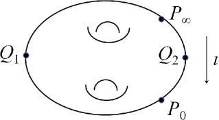
Figure 1: Algebraic curve $\Gamma$ with involution.

3 Algebraic-geometrical solutions

Consider algebraic-geometrical solutions of the Toda hierarchy constructed from a genus $g$ algebraic curve admitting holomorphic involution $\iota$ with two fixed points $Q_{1}$, $Q_{2}$ and an effective degree $g$ divisor satisfying the condition (3.4) below. Let $P_{\infty}$, $P_{0}$ be two marked points (different from $Q_{1}$, $Q_{2}$) such that $P_{0}=\iota P_{\infty}$ with local parameters $k^{-1}$ and $k=\iota(k^{-1})$ respectively (Fig. 1). In this section we denote the set of independent variables of the hierarchy as ${\bf t}=(t_{1},t_{2},\ldots)$ (we set $\bar{t}_{k}=-t_{k}$ in the full 2D Toda hierarchy and put $T_{k}=t_{k}$). Set

$$U^{\alpha}({\bf t})=\sum_{j\geq 1}t_{j}(U_{j}^{\alpha}+U_{j}^{\alpha+g_{0}})\quad\mbox{or}\quad\vec{U}({\bf t})=\sum_{j\geq 1}t_{j}(\vec{U}_{j}-\iota\vec{U}_{j}).$$ (3.1)

Here and below we use the notation introduced in the appendix.

The Baker-Akhiezer function has the form

$$\begin{array}[]{l}\displaystyle{\Psi(n,{\bf t},P)=\exp\Bigl{(}\sum_{k}t_{k}(\Omega_{k}(P)-\Omega_{k}(\iota P))+n\Omega_{0}(P)\Bigr{)}}\\ \\ \phantom{aaaaaaaaaaaaaaaaaaa}\displaystyle{\times\,\frac{\Theta(\vec{A}(P)+n\vec{U}_{0}+\vec{U}({\bf t})+\vec{Z})\Theta(\vec{Z})}{\Theta(\vec{A}(P)+\vec{Z})\Theta(n\vec{U}_{0}+\vec{U}({\bf t})+\vec{Z})}},\end{array}$$ (3.2)

where the vector $\vec{Z}$ is given by

$$\vec{Z}=-\vec{A}({\cal D})-\vec{K}.$$ (3.3)

Here ${\cal D}$ is an effective non-special divisor of degree $g$ and $\vec{K}$ is the vector of Riemann’s constants. The function $\Psi(n,{\bf t},P)$ has poles at the points of the divisor ${\cal D}$. We assume that the divisor ${\cal D}$ is subject to the condition

$${\cal D}+\iota{\cal D}={\cal K}+Q_{1}+Q_{2},$$ (3.4)

where ${\cal K}$ is the canonical class. This relation is equivalent to

$$\vec{A}({\cal D})+\vec{A}(\iota{\cal D})+2\vec{K}=\vec{A}(Q_{1})+\vec{A}(Q_{2}).$$ (3.5)

Note that with out choice of the initial point of the Abel map we have $\vec{A}(Q_{1})=0$. The Baker-Akhiezer function (3.2) is normalized in such a way that

$$\Psi(n,{\bf t},Q_{1})=1.$$ (3.6)

Near the points $P_{\infty}$, $P_{0}$ it has essential singularities of the form

$$\begin{array}[]{l}\Psi(n,{\bf t},P)=e^{\varphi_{+}(n)}k^{n}e^{\xi({\bf t},k)}\Bigl{(}1+O(k^{-1})\Bigr{)},\quad P\to P_{\infty}\quad(k\to\infty),\\ \\ \Psi(n,{\bf t},P)=e^{\varphi_{-}(n)}k^{n}e^{-\xi({\bf t},k^{-1})}\Bigl{(}1+O(k)\Bigr{)},\quad P\to P_{0}\quad(k\to 0).\end{array}$$ (3.7)

From the explicit formula (3.2) we have

$$\begin{array}[]{l}\displaystyle{e^{\varphi_{+}(n)}=\frac{\Theta(\vec{A}(P_{\infty})+n\vec{U}_{0}+\vec{U}({\bf t})+\vec{Z})\Theta(\vec{Z})}{\Theta(\vec{A}(P_{\infty})+\vec{Z})\Theta(n\vec{U}_{0}+\vec{U}({\bf t})+\vec{Z})}\,\exp\Bigl{(}-\!\sum_{k}\Omega_{k}(P_{0})t_{k}\Bigr{)}},\\ \\ \displaystyle{e^{\varphi_{-}(n)}=\frac{\Theta(\vec{A}(P_{0})+n\vec{U}_{0}+\vec{U}({\bf t})+\vec{Z})\Theta(\vec{Z})}{\Theta(\vec{A}(P_{0})+\vec{Z})\Theta(n\vec{U}_{0}+\vec{U}({\bf t})+\vec{Z})}\,\exp\Bigl{(}\,\sum_{k}\Omega_{k}(P_{0})t_{k}\Bigr{)}}.\end{array}$$ (3.8)

The dual Baker-Akhiezer function $\Psi^{*}(n,{\bf t},P)$ can be introduced as follows. Let $d\Omega(P)$ be the meromorphic differential with simple poles at the points $P_{0}$, $P_{\infty}$ with residues $\pm 1$ and zeros at the points of the divisor ${\cal D}$. This differential has other $g$ zeros at the points of some effective divisor ${\cal D}^{*}$ such that

$${\cal D}+{\cal D}^{*}={\cal K}+P_{0}+P_{\infty},$$ (3.9)

or

$$\vec{A}({\cal D})+\vec{A}({\cal D}^{*})+2\vec{K}=\vec{A}(P_{0})+\vec{A}(P_{\infty}).$$ (3.10)

The dual Baker-Akhiezer function is a unique function with poles at the points of the divisor ${\cal D}^{*}$ and essential singularities of the form

$$\begin{array}[]{l}\Psi^{*}(n,{\bf t},P)=e^{-\varphi_{+}(n)}k^{-n}e^{-\xi({\bf t},k)}\Bigl{(}1+O(k^{-1})\Bigr{)},\quad P\to P_{\infty}\quad(k\to\infty),\\ \\ \Psi^{*}(n,{\bf t},P)=e^{-\varphi_{-}(n)}k^{-n}e^{\xi({\bf t},k^{-1})}\Bigl{(}1+O(k)\Bigr{)},\quad P\to P_{0}\quad(k\to 0).\end{array}$$ (3.11)

Theorem 3.1

The Baker-Akhiezer function and its dual obey the bilinear relation

$$\mathop{\hbox{res}}\limits_{P=P_{0}}\Bigl{(}\Psi(n,{\bf t},P)\Psi^{*}(n^{\prime},{\bf t}^{\prime},P)d\Omega(P)\Bigr{)}+\mathop{\hbox{res}}\limits_{P=P_{\infty}}\Bigl{(}\Psi(n,{\bf t},P)\Psi^{*}(n^{\prime},{\bf t}^{\prime},P)d\Omega(P)\Bigr{)}=0$$ (3.12)

for all $n,n^{\prime}$, ${\bf t},{\bf t^{\prime}}$.

Proof. The differential $\Psi(n,{\bf t},P)\Psi^{*}(n^{\prime},{\bf t}^{\prime},P)d\Omega(P)$ is a well-defined differential on $\Gamma$. From the definition of $d\Omega$ it follows that it has singularities only at the points $P_{0}$, $P_{\infty}$. Therefore, sum of the residues must be zero.  

Remark 3.1

The bilinear relation (2.19) is the realization of (3.12) written in the local parameter.

Let $d\hat{\Omega}(P)$ be the meromorphic differential with simple poles at the points $Q_{1}$, $Q_{2}$ with residues $\pm 1$ and zeros at the points of the divisor ${\cal D}+\iota{\cal D}$. Such differential is unique. It is given by the explicit formula

$$\begin{array}[]{l}\displaystyle{d\hat{\Omega}(P)=\frac{C\,\Theta_{*}(\vec{A}(Q_{2})-\vec{A}(Q_{1}))}{\Theta(\vec{Z})\Theta(\vec{A}(Q_{1})-\vec{A}(Q_{2})-\vec{Z})}}\\ \\ \phantom{aaaaaaaaaaaaaaa}\displaystyle{\times\,\frac{\Theta(\vec{A}(P)-\vec{A}(Q_{1})+\vec{Z})\Theta(\vec{A}(P)-\vec{A}(Q_{2})-\vec{Z})}{\Theta_{*}(\vec{A}(P)-\vec{A}(Q_{1}))\Theta_{*}(\vec{A}(P)-\vec{A}(Q_{2}))}}\,\,d\zeta(P),\end{array}$$ (3.13)

where $C$ is a constant depending only on the point $P_{\infty}$ and $d\zeta$ is the holomorphic differential

$$d\zeta(P)=\sum_{\alpha=1}^{g}\Theta_{*,\alpha}(0)d\omega_{\alpha}(P)$$ (3.14)

and $\Theta_{*}$ is the odd theta-function with some odd half-integer characteristics. It is known [22] that the differential $d\zeta$ has $g-1$ double zeros at the points, where the function $\Theta_{*}(\vec{A}(P)-\vec{A}(Q))$ has simple zeros other than the zero at $P=Q$ (they are independent of $Q$).

Consider the differential

$$d\hat{\Omega}(n,{\bf t},P)=\Psi(n,{\bf t},P)\Psi(n,{\bf t},\iota P)d\hat{\Omega}(P).$$

It is a well-defined meromorphic differential with simple poles at the points $Q_{1}$, $Q_{2}$ and no other singularities. Therefore,

$$1=\mathop{\hbox{res}}\limits_{P=Q_{1}}d\hat{\Omega}(n,{\bf t},P)=-\mathop{\hbox{res}}\limits_{P=Q_{2}}d\hat{\Omega}(n,{\bf t},P)=\Psi^{2}(n,{\bf t},Q_{2}),$$ (3.15)

i.e., $\Psi(n,{\bf t},Q_{2})=\pm 1$.

Lemma 3.1

It holds

$$\Psi(n,{\bf t},Q_{2})=(-1)^{n}.$$ (3.16)

Proof. First consider the case $n=0$. Since the Baker-Akhiezer function is continuous in ${\bf t}$ and $\Psi(0,0,Q_{2})=1$, we conclude that $\Psi(0,{\bf t},Q_{2})=1$. Next consider the case $n=1$. The correct sign can be determined by the following argument. The function $\Psi(1,{\bf t},Q_{2})$ is continuous in ${\bf t}$ and $P_{\infty}$ for $P_{\infty}\neq Q_{1}$. Therefore, in order to find the correct sign, we set ${\bf t}=0$ and choose $P_{\infty}$ in a neighborhood of $Q_{1}$ with some local parameter $z^{-1}$ which is odd under the involution. By the definition of $\Omega_{0}(P)$ we have

$$e^{\Omega_{0}(P)}=\frac{z(P)-z(P_{\infty})}{z(P)+z(P_{\infty})}\,\Bigl{(}1+O(z^{-1}(P))\Bigr{)}.$$

For any fixed positive $r\ll 1$ one can choose $\eta$ such that for $|z^{-1}(P_{\infty})|<\eta$ and $|z^{-1}(P)|=r$ the inequality $\Bigl{|}1+e^{\Omega_{0}(P)}\Bigr{|}<M\eta$ holds with a constant $M$ independent of $\eta$. Moreover, for any fixed path from a point $P^{\prime}$, $|z^{-1}(P^{\prime})|=r$, to $Q_{2}$ there exists a constant $M_{1}$ (which depends on the path but does not depend on $\eta$) such that the inequality $\displaystyle{\Bigl{|}\int_{P^{\prime}}^{Q_{2}}d\Omega_{0}\Bigr{|}<M_{1}\eta}$ holds. It then follows that for a fixed path from $Q_{1}$ to $Q_{2}$

$$\lim_{P_{\infty}\to Q_{1}}e^{\Omega_{0}(Q_{2})}=-1.$$ (3.17)

In fact if we define $\displaystyle{\tilde{\Omega}_{0}(P)=\int_{Q_{0}}^{P}d\Omega_{0}}$ with some initial point $Q_{0}\to Q_{1}$, then the result depends on the order of the limits:

$$\lim_{Q_{0}\to Q_{1}}\lim_{P_{\infty}\to Q_{1}}e^{\tilde{\Omega}_{0}(Q_{2})}=1\quad\mbox{but}\quad\lim_{P_{\infty}\to Q_{1}}\lim_{Q_{0}\to Q_{1}}e^{\tilde{\Omega}_{0}(Q_{2})}=-1,$$

and our case is the latter limit. The ratio of theta-functions is a continuous function of $P_{\infty}$ which tends to $1$ as $P_{\infty}\to Q_{1}$ and the formula (3.16) for $n=1$ is proved. The statement of the lemma for arbitrary $n$ follows from equation (3.17).  

The following theorem is the key for constructing the algebraic-geometrical solutions of the Toda hierarchy with the constraint of type B.

Theorem 3.2

Let $\Gamma$ be an algebraic curve with involution $\iota$ having two fixed points $Q_{1},Q_{2}$, and let $\vec{Z}$ be a vector such that

$$\vec{Z}+\iota\vec{Z}=-\vec{A}(Q_{1})-\vec{A}(Q_{2}).$$ (3.18)

Then the following identity holds:

$$\begin{array}[]{l}\Theta^{2}(\vec{A}(P)\!+\!\vec{Z})=c(P)\Theta(\vec{A}(P)\!-\!\vec{A}(\iota P)\!+\!\vec{Z})\Theta(\vec{Z}),\end{array}$$ (3.19)

where $c(P)$ is some constant depending only on $P$.

Proof. Consider the differential

$$d\tilde{\Omega}(n,{\bf t},P)=\Psi(n+1,{\bf t},P)\Psi(n,{\bf t},\iota P)d\Omega(P).$$

It is a well-defined meromorphic differential with simple poles at the points $Q_{1}$, $Q_{2}$, $P_{\infty}$ and no other singularities. The sum of its residues must be zero. Therefore,

$$\mathop{\hbox{res}}\limits_{P=P_{\infty}}d\tilde{\Omega}(n,{\bf t},P)=2$$ (3.20)

since the residues at the points $Q_{1,2}$ are equal to $-1$. We have:

$$\mathop{\hbox{res}}\limits_{P=P_{\infty}}d\tilde{\Omega}(n,{\bf t},P)=e^{\varphi_{+}(n+1)+\varphi_{-}(n)}\,\frac{\tilde{C}\,\Theta_{*}(\vec{A}(Q_{2}))\Theta(\vec{A}(P_{\infty})\!+\!\vec{Z})\Theta(\vec{A}(P_{\infty})\!-\!\vec{A}(Q_{2})\!-\!\vec{Z})}{\Theta_{*}(\vec{A}(P_{\infty}))\Theta_{*}(\vec{A}(P_{\infty})-\vec{A}(Q_{2}))\Theta(\vec{Z})\Theta(\vec{A}(Q_{2})\!+\!\vec{Z})}$$ (3.21)

with some constant $\tilde{C}$ depending only on $P_{\infty}$. Substituting here $e^{\varphi_{\pm}(n)}$ from (3.8) and using (A19), we obtain:

$$\frac{\tilde{C}(P_{\infty})\,A(P_{\infty},\vec{Z})\,\Theta^{2}(\vec{A}(P_{0})+n\vec{U}_{0}+\vec{U}({\bf t})+\vec{Z})}{\Theta(\vec{A}(P_{0})-\vec{A}(\iota P_{0})+n\vec{U}_{0}+\vec{U}({\bf t})+\vec{Z})\Theta(n\vec{U}_{0}+\vec{U}({\bf t})+\vec{Z})}=2,$$ (3.22)

where

$$A(P_{\infty},\vec{Z})=\frac{\Theta(\vec{A}(P_{\infty})-\vec{A}(Q_{2})-\vec{Z})\Theta(\vec{Z})}{\Theta(\vec{A}(Q_{2})+\vec{Z})\,\Theta(\vec{A}(P_{0})+\vec{Z})}.$$ (3.23)

Some additional arguments based on the behavior of the theta-functions under involution show that in fact $A(P_{\infty},\vec{Z})=1$. Therefore, we have obtained the identity

$$\begin{array}[]{l}\Theta^{2}(\vec{A}(P_{0})\!+\!n\vec{U}_{0}\!+\!\vec{U}({\bf t})\!+\!\vec{Z})\\ \\ \phantom{aaaaaaaaaaaa}=c(P_{0})\Theta(\vec{A}(P_{0})\!-\!\vec{A}(\iota P_{0})\!+\!n\vec{U}_{0}\!+\!\vec{U}({\bf t})\!+\!\vec{Z})\Theta(n\vec{U}_{0}\!+\!\vec{U}({\bf t})\!+\!\vec{Z}).\end{array}$$ (3.24)

Now, putting $P_{0}=P$, $n={\bf t}=0$ and noting that (3.5) with $\vec{Z}=\vec{A}({\cal D})-\vec{K}$ implies that $\vec{Z}+\iota\vec{Z}=-\vec{A}(Q_{1})-\vec{A}(Q_{2})$, we arrive at (3.19). Note that $\iota\vec{U}_{0}=-\vec{U}_{0}$, $\iota\vec{U}({\bf t})=-\vec{U}({\bf t})$, so the vector $\vec{Z}_{n,{\bf t}}=\vec{Z}+n\vec{U}_{0}+\vec{U}({\bf t})$ still satisfies the condition (3.18).  

Corollary 3.1

Under the assumptions of Theorem 3.2, it holds:

$$\Theta(\vec{A}(P)\!+\!\vec{Z})=c_{1}(P)\,\Theta_{\rm Pr}(\vec{A}^{\rm Pr}(P)+\vec{z})\,\Theta_{\rm Pr}(\vec{z}),$$ (3.25)

where $\vec{z}=\sigma^{-1}(\vec{Z}+\frac{1}{2}\vec{A}(Q_{2}))$ and the map $\sigma$ is defined in (A24).

Proof. The condition (3.5) can be rewritten as

$$\begin{array}[]{c}\iota\Bigl{(}\vec{Z}+\frac{1}{2}\vec{A}(Q_{2})\Bigr{)}=-\Bigl{(}\vec{Z}+\frac{1}{2}\vec{A}(Q_{2})\Bigr{)},\end{array}$$

so the map $\sigma^{-1}(\vec{Z}+\frac{1}{2}\vec{A}(Q_{2})):=\vec{z}\in\mbox{\Bbb C}^{g_{0}}$ is well-defined. The same is true for the map $\sigma^{-1}(\vec{A}(P)-\vec{A}(\iota P)+\vec{Z}+\frac{1}{2}\vec{A}(Q_{2}))=\vec{A}^{\rm Pr}(P)+\vec{z}$, where $\vec{A}^{\rm Pr}(P)$ is the Abel-Prym map (A26). Then, taking the square root of both sides of identity (3.19) and using (A28), we arrive at (3.25).  

Restoring the dependence on $n$ and ${\bf t}$ in (3.25), we can write it in the form

$$\Theta(\vec{A}(P_{0})\!+\!n\vec{U}_{0}\!+\!\vec{U}({\bf t})\!+\!\vec{Z})=c_{1}(P_{0})\,\Theta_{\rm Pr}((n+1)\vec{u}_{0}\!+\!\vec{u}({\bf t})\!+\!\vec{z})\,\Theta_{\rm Pr}(n\vec{u}_{0}\!+\!\vec{u}({\bf t})\!+\!\vec{z}),$$ (3.26)

where $\vec{u}_{0}=\vec{A}^{\rm Pr}(P_{0})$, $\vec{u}({\bf t})=\sigma^{-1}(\vec{U}({\bf t}))$.

Theorem 3.3

The Baker-Akhiezer function (3.2) satisfies the bilinear identity

$$\begin{array}[]{l}\displaystyle{\mathop{\hbox{res}}\limits_{P=P_{0}}\Bigl{(}\Psi(n,{\bf t},P)\Psi(n^{\prime},{\bf t}^{\prime},\iota P)d\hat{\Omega}(P)\Bigr{)}}\\ \\ \phantom{aaaaaaaaaaaaaaaaa}\displaystyle{+\mathop{\hbox{res}}\limits_{P=P_{\infty}}\Bigl{(}\Psi(n,{\bf t},P)\Psi(n^{\prime},{\bf t}^{\prime},\iota P)d\hat{\Omega}(P)\Bigr{)}=1-(-1)^{n-n^{\prime}}}\end{array}$$ (3.27)

for all $n,n^{\prime}$, ${\bf t},{\bf t^{\prime}}$.

Proof. The differential $\Psi(n,{\bf t},P)\Psi(n^{\prime},{\bf t}^{\prime},\iota P)d\hat{\Omega}(P)$ is a well-defined differential on $\Gamma$ with essential singularities at the points $P_{0}$, $P_{\infty}$ and simple poles at the points $Q_{1}$, $Q_{2}$. Equation (3.27) is the statement that sum of its residues is equal to zero.  

The next theorem establishes the connection between the dual Baker-Akhiezer function $\Psi^{*}(n,P)$ and the function $\Psi(n,\iota P)$.

Theorem 3.4

The following identity holds:

$$\Psi^{*}(n,P)d\Omega(P)=A\Bigl{(}\Psi(n\!+\!1,\iota P)-\Psi(n\!-\!1,\iota P)\Bigr{)}d\hat{\Omega}(P)$$ (3.28)

with some constant $A$.

Remark 3.2

Equation (3.28) implies that subtracting the bilinear identities of the form (3.27) taken at $n^{\prime}+1$ and $n^{\prime}-1$, we get the bilinear identity (3.12).

Proof of Theorem 3.4. Let us show that poles and zeros of the differentials in both sides of (3.28) coincide. Both sides of (3.28) have essential singularities at the points $P_{0},P_{\infty}$ and the exponential factors at these singularities coincide. Besides, there is a pole of order $n+1$ at $P_{0}$ in the left hand side of (3.28), and the differential is holomorphic in all other points. It is easy to see that the differential in the right hand side has the same singularity. Possible poles at $Q_{1}$, $Q_{2}$ cancel because $\Psi(n\!+\!1,Q_{1,2})=\Psi(n\!-\!1,Q_{1,2})$ (see (3.16)). As far as zeros are concerned, both sides have a zero of order $n-1$ (here we assume that $n\geq 1$) and $g$ simple zeros at the points of the divisor ${\cal D}$. The linear space of such differentials is one-dimensional, whence the two sides of (3.28) are proportional to each other. In order to find the coefficient of proportionality, we compare the leading terms of $\Psi^{*}(n,P)$ and $\Psi(n\!+\!1,\iota P)-\Psi(n\!-\!1,\iota P)$ at $P_{0}$. The coefficients at the leading terms are $e^{-\varphi_{-}(n)}$ and $e^{\varphi_{+}(n+1)}$ respectively. From the proof of Theorem 3.2 (see (3.20), (3.21)) it follows that

$$e^{\varphi_{+}(n+1)+\varphi_{-}(n)}=\mbox{const}.$$ (3.29)

Therefore, the coefficient of proportionality $A$ does not depend on $n$.  

The Baker-Akhiezer function is an eigenfunction of the Lax operators:

$$L\Psi(n,P)=k\Psi(n,P),\qquad\bar{L}\Psi(n,\iota P)=k\Psi(n,\iota P)$$ (3.30)

and

$$L^{{\dagger}}\Psi^{*}(n,P)=k\Psi^{*}(n,P).$$ (3.31)

It is easy to see that our normalization of the Baker-Akhiezer function corresponds to the balanced gauge. Indeed, writing $L=a(n)e^{\partial_{n}}+\ldots$, $\bar{L}=\bar{a}(n)e^{-\partial_{n}}+\ldots$, and comparing the leading terms in (3.30), we have:

$$a(n)e^{\varphi_{+}(n+1)-\varphi_{+}(n)}=1,\quad\bar{a}(n)e^{\varphi_{-}(n-1)-\varphi_{-}(n)}=1.$$

Therefore,

$$\frac{\bar{a}(n)}{a(n)}=e^{\varphi_{-}(n)-\varphi_{-}(n-1)-\varphi_{+}(n)+\varphi_{+}(n+1)}=1$$

due to (3.29). The following corollary from Theorem 3.4 states that the $L$-operators obey the constraint of type B.

Corollary 3.2

The constraint (2.22) for the $L$-operators of the Toda lattice in the balanced gauge holds.

Proof. Using (3.28), we can write

$$\Psi^{*}(n,P)=A^{\prime}(P)\Bigl{(}\Psi(n\!+\!1,\iota P)-\Psi(n\!-\!1,\iota P)\Bigr{)},$$

where $\displaystyle{A^{\prime}(P)=A\frac{d\hat{\Omega}(P)}{d\Omega(P)}}$. Therefore (see (3.30), (3.31)),

$$\bar{L}(n+1)\Psi(n+1,\iota P)-\bar{L}(n-1)\Psi(n-1,\iota P)=k\Bigl{(}\Psi(n+1,\iota P)-\Psi(n-1,\iota P)\Bigr{)}$$

$$=k(A^{\prime}(P))^{-1}\Psi^{*}(n,P)=(A^{\prime}(P))^{-1}L^{{\dagger}}(n)\Psi^{*}(n,P)$$

$$=L^{{\dagger}}(n)\Bigl{(}\Psi(n+1,\iota P)-\Psi(n-1,\iota P)\Bigr{)}.$$

or

$$\Bigl{(}\bar{L}(n+1)-L^{{\dagger}}(n)\Bigr{)}\Psi(n+1,\iota P)=\Bigl{(}\bar{L}(n-1)-L^{{\dagger}}(n)\Bigr{)}\Psi(n-1,\iota P).$$

Since this is true for any $P$, the equality should hold for the operators, i.e.,

$$\Bigl{(}\bar{L}(n+1)-L^{{\dagger}}(n)\Bigr{)}e^{\partial_{n}}=\Bigl{(}\bar{L}(n-1)-L^{{\dagger}}(n)\Bigr{)}e^{-\partial_{n}},$$

which is (2.22).  

Comparing with the standard gauge, we can write:

$$e^{\varphi(n)}=e^{\varphi_{-}(n)-\varphi_{+}(n)}=g(n)g(n+1).$$ (3.32)

In terms of the tau-function we have:

$$e^{\varphi(n)}=\frac{\tau(n+1)}{\tau(n)}=\frac{\tau^{B}(n+1)}{\tau^{B}(n-1)},$$ (3.33)

where $\tau^{B}(n)=\tau^{B}(n,{\bf t})$ is the tau-function of the Toda hierarchy with the constraint of type B introduced in (2.43). This tau-function is connected with the tau-function of the Toda lattice by the relation (2.46).

The algebraic-geometrical solutions of the Toda lattice were constructed by one of the authors in [23] using the general method suggested in [24, 25]. Restricting to the subspace $t_{k}+\bar{t}_{k}=0$, we can write the tau-function:

$$\tau(n,{\bf t})=e^{-L(n,{\bf t})-Q(n,{\bf t})}\Theta\Bigl{(}\vec{A}(P_{\infty})+n\vec{U}_{0}+\vec{U}({\bf t})+\vec{Z}\Bigr{)},$$ (3.34)

where $L(n,{\bf t})$ is an inessential linear form in $n$, ${\bf t}$ and $Q(n,{\bf t})$ is the quadratic form

$$Q(n,{\bf t})=\sum_{i,j}(\Omega_{ij}-\omega_{ij})t_{i}t_{j}-2n\sum_{j}\Omega_{j}(P_{0})t_{j}$$ (3.35)

($\Omega_{ij}$ and $\omega_{ij}$ are coefficients of expansions of the function $\Omega_{i}(P)$ near $P_{\infty}$ and $P_{0}$, see (A12), (A17)). Then $e^{\varphi(n)}$ is given by

$$e^{\varphi(n)}=\exp\Bigl{(}2\sum_{j}\Omega_{j}(P_{0})t_{j}\Bigr{)}\frac{\Theta(\vec{A}(P_{\infty})+\vec{Z})}{\Theta(\vec{A}(P_{0})+\vec{Z})}\,\frac{\Theta(\vec{A}(P_{0})+n\vec{U}_{0}+\vec{U}({\bf t})+\vec{Z})}{\Theta(\vec{A}(P_{\infty})+n\vec{U}_{0}+\vec{U}({\bf t})+\vec{Z})}.$$ (3.36)

Using equation (3.26), we find the tau-function of the Toda lattice with the constraint:

$$\tau^{B}(n,{\bf t})=e^{-L^{B}(n,{\bf t})-\frac{1}{2}\,Q(n,{\bf t})}\Theta_{\rm Pr}\Bigl{(}n\vec{u}_{0}+\vec{u}({\bf t})+\vec{z}\Bigr{)},$$ (3.37)

where $\vec{u}_{0}=\vec{A}^{\rm Pr}(P_{0})$, $\vec{u}({\bf t})=\sigma^{-1}(\vec{U}({\bf t}))$ and $L^{B}(n,{\bf t})$ is an inessential linear form. The formulas

$$v(n)=\frac{\tau^{B}(n+1)\tau^{B}(n-1)}{(\tau^{B}(n))^{2}},$$ (3.38)

$$f_{0}(n)=\frac{\tau^{B}(n+1)\tau^{B}(n-1)}{(\tau^{B}(n))^{2}}\,\partial_{t_{1}}\!\log\frac{\tau^{B}(n+1)}{\tau^{B}(n-1)}$$ (3.39)

provide a solution to equations (2.37).

Remark 3.3

For algebraic-geometrical solutions, the discrete variable $n$ can be regarded as a continuous variable, as equation (3.37) suggests. The Baker-Akhiezer functions then have a discontinuity on a cut between the points $P_{0}$ and $P_{\infty}$. The right hand side of equation (3.16) should then be $e^{i\pi n}$.

4 Concluding remarks

We have introduced a subhierarchy of the 2D Toda lattice by imposing the constraint of the form (2.22) on the two Lax operators. Restricting the dynamics to the subspace $t_{k}+\bar{t}_{k}=0$ of the space of independent variables, we have shown that this constraint is invariant under flows of the Toda hierarchy. The hierarchy which is obtained in this way can be regarded as an integrable discretization of the BKP hierarchy. We have also constructed its algebraic-geometrical solutions in terms of Prym theta-functions.

Along with the CKP and BKP hierarchies, in [6] a whole family of subhierarchies of KP indexed by $m\in\mbox{\Bbb Z}_{\geq 0}$ was introduced of which $m=0$ ($m=1$) case corresponds to the BKP (CKP) hierarchy. They are defined by imposing a constraint of the type

$$(L^{\rm KP})^{{\dagger}}=-Q^{-1}_{m}L^{\rm KP}Q_{m}$$ (4.1)

on the Lax operator $L^{\rm KP}$ of the KP hierarchy. Here

$$Q_{m}=\partial_{x}^{m-1}+\mbox{lower order terms}$$

is a difference operator of order $m-1$ such that

$$Q_{m}^{{\dagger}}=(-1)^{m-1}Q_{m}$$ (4.2)

(at $m=0$ one sets $Q_{0}=\partial_{x}^{-1}$). It was also shown that in the case $m=2$ ($Q_{2}=\partial_{x}$) one obtains a hierarchy which is equivalent to BKP. To the best of our knowledge, nothing is known about the cases $m\geq 3$.

It would be interesting to investigate whether more general constraints analogous to (4.1) exist in the Toda case. Hypothetically, they might have the form

$$L^{{\dagger}}=S^{-1}_{m}\bar{L}S_{m},$$ (4.3)

where $S_{m}$ is a difference operator (a finite linear combination of powers of $e^{\partial_{n}}-e^{-\partial_{n}}$ with some coefficients) of order $m-1$ such that

$$S_{m}^{{\dagger}}=(-1)^{m-1}S_{m}.$$

At $m=0$ we set $S_{0}=(e^{\partial_{n}}-e^{-\partial_{n}})^{-1}$, then the case $m=0$ ($m=1$) corresponds to the Toda hierarchy with the constraint of type B discussed in this paper (respectively, the Toda hierarchy with the constraint of type C [5]). Presumably, in the case $m=2$ one obtains a hierarchy which is equivalent to the Toda lattice of type B.

Appendix: Algebraic curves, differentials and theta-functions

Here we present the basic notions and facts related to algebraic curves (Riemann surfaces) [20, 21] and theta-functions [22] which are necessary for the construction of quasi-periodic solutions to the Toda hierarchy.

Matrix of periods.

Let $\Gamma$ be a smooth compact algebraic curve of genus $g$. We fix a canonical basis of cycles ${\sf a}_{\alpha},{\sf b}_{\alpha}$ ($\alpha=1,\ldots,g$) with the intersections ${\sf a}_{\alpha}\circ{\sf a}_{\beta}={\sf b}_{\alpha}\circ{\sf b}_{\beta}=0$, ${\sf a}_{\alpha}\circ{\sf b}_{\beta}=\delta_{\alpha\beta}$ and a basis of holomorphic differentials $d\omega_{\alpha}$ normalized by the condition $\displaystyle{\oint_{{\sf a}_{\alpha}}d\omega_{\beta}=\delta_{\alpha\beta}}$. The matrix of periods is defined as

$$T_{\alpha\beta}=\oint_{{\sf b}_{\alpha}}d\omega_{\beta},\qquad\alpha,\beta=1,\ldots,g.$$ (A1)

It is a symmetric matrix with positively defined imaginary part. The Jacobian of the curve $\Gamma$ is the $g$-dimensional complex torus

$$J(\Gamma)=\mbox{\Bbb C}^{g}/\{\vec{N}+T\vec{M}\},$$ (A2)

where $\vec{N}$, $\vec{M}$ are $g$-dimensional vectors with integer components.

Riemann theta-functions.

The Riemann theta-function associated with the Riemann surface is defined by the absolutely convergent series

$$\Theta(\vec{z})=\Theta(\vec{z}|T)=\sum_{\vec{n}\in\raise-1.0pt\hbox{$\mbox{\Bbbb Z}$}^{g}}e^{\pi i(\vec{n},T\vec{n})+2\pi i(\vec{n},\vec{z})},$$ (A3)

where $T$ is the matrix of periods, $\vec{z}=(z_{1},\ldots,z_{g})$ and $\displaystyle{(\vec{n},\vec{z})=\sum_{\alpha=1}^{g}n_{\alpha}z_{\alpha}}$. It is an entire function with the following quasi-periodicity property:

$$\Theta(\vec{z}+\vec{N}+T\vec{M})=\exp(-\pi i(\vec{M},T\vec{M})-2\pi i(\vec{M},\vec{z}))\Theta(\vec{z}).$$ (A4)

More generally, one can introduce the theta-functions with characteristics $\vec{\delta}^{\prime}$, $\vec{\delta}^{\prime\prime}$:

$$\Theta\left[\begin{array}[]{c}\vec{\delta}^{\prime}\\ \vec{\delta}^{{}^{\prime\prime}}\end{array}\right](\vec{z})=\sum_{\vec{n}\in\raise-1.0pt\hbox{$\mbox{\Bbbb Z}$}^{g}}e^{\pi i(\vec{n}+\vec{\delta}^{\prime},T(\vec{n}+\vec{\delta}^{\prime}))+2\pi i(\vec{n}+\vec{\delta}^{\prime},\vec{z}+\vec{\delta}^{\prime\prime})}.$$ (A5)

Half-integer characteristics play an especially important role. Let $\displaystyle{\left[\begin{array}[]{c}\vec{\delta}^{\prime}\\ \vec{\delta}^{\prime\prime}\end{array}\right]}$ be an odd half-integer characteristics, i.e. such that $(-1)^{4((\vec{\delta}^{\prime},\vec{\delta}^{\prime\prime})}=-1$. For brevity, by $\Theta_{*}$ we denote the corresponding odd theta-function: $\displaystyle{\Theta\left[\begin{array}[]{c}\vec{\delta}^{\prime}\\ \vec{\delta}^{{}^{\prime\prime}}\end{array}\right](\vec{z})}:=\Theta_{*}(\vec{z})$, $\Theta_{*}(-\vec{z})=-\Theta_{*}(\vec{z})$.

The Abel map.

The Abel map $\vec{A}(P)$, $P\in\Gamma$ from $\Gamma$ to $J(\Gamma)$ is defined as

$$\vec{A}(P)=\int_{Q_{1}}^{P}d\vec{\omega},\qquad d\vec{\omega}=(d\omega_{1},\ldots,d\omega_{g}).$$ (A6)

The Abel map can be extended to the group of divisors ${\cal D}=n_{1}P_{1}+\ldots+n_{K}P_{K}$ as

$$\vec{A}({\cal D})=\sum_{i=1}^{K}n_{i}\int_{Q_{1}}^{P_{i}}d\vec{\omega}=\sum_{i=1}^{K}n_{i}\vec{A}(P_{i}).$$ (A7)

Consider the function $f(P)=\Theta(\vec{A}(P)-\vec{e})$ and assume that it is not identically zero. It can be shown that this function has $g$ zeros on $\Gamma$ at a divisor ${\cal D}=Q_{1}+\ldots+Q_{g}$ and $\vec{A}({\cal D})=\vec{e}-\vec{K}$, where $\vec{K}=(K_{1},\ldots,K_{g})$ is the vector of Riemann’s constants

$$K_{\alpha}=\pi i+\pi iT_{\alpha\alpha}-2\pi i\sum_{\beta\neq\alpha}\oint_{a_{\beta}}\omega_{\alpha}(P)d\omega_{\beta}(P).$$ (A8)

In other words, for any non-special effective divisor ${\cal D}=Q_{1}+\ldots+Q_{g}$ of degree $g$ the function

$$f(P)=\Theta\Bigl{(}\vec{A}(P)-\vec{A}({\cal D})-\vec{K}\Bigr{)}$$

has exactly $g$ zeros at the points $Q_{1},\ldots,Q_{g}$. Let ${\cal K}$ be the canonical class of divisors (the equivalence class of divisors of poles and zeros of abelian differentials on $\Gamma$), then one can show that

$$2\vec{K}=-\vec{A}({\cal K}).$$ (A9)

It is known that $\mbox{deg}\,{\cal K}=2g-2$. In particular, this means that holomorphic differentials have $2g-2$ zeros on $\Gamma$.

The Riemann bilinear identity.

Let ${\sf a}_{\alpha}$, ${\sf b}_{\alpha}$ be Jordan arcs which represent the canonical basis of cycles intersecting transversally at a single point and let

$$\tilde{\Gamma}=\Gamma\setminus\bigcup_{\alpha}\Bigl{(}{\sf a}_{\alpha}\bigcup{\sf b}_{\alpha}\Bigr{)}$$

be a simply connected subdomain of $\Gamma$ (a fundamental domain). Integrals of any two meromorphic differentials $d\Omega^{\prime}$, $d\Omega^{\prime\prime}$ satisfy the Riemann bilinear identity

$$\oint_{\partial\tilde{\Gamma}}\Bigl{(}\int_{Q_{1}}^{P}d\Omega^{\prime}\Bigr{)}d\Omega^{\prime\prime}(P)=\sum_{\alpha=1}^{g}\left(\oint_{{\sf a}_{\alpha}}d\Omega^{\prime}\oint_{{\sf b}_{\alpha}}d\Omega^{\prime\prime}-\oint_{{\sf b}_{\alpha}}d\Omega^{\prime}\oint_{{\sf a}_{\alpha}}d\Omega^{\prime\prime}\right).$$ (A10)

In particular, if ${\sf a}$-periods of both differentials are equal to zero, we have

$$\oint_{\partial\tilde{\Gamma}}\Bigl{(}\int_{Q_{1}}^{P}d\Omega^{\prime}\Bigr{)}d\Omega^{\prime\prime}(P)=0.$$ (A11)

Differentials of the second and third kind.

Let $P_{\infty}\in\Gamma$ be a marked point and $k^{-1}$ a local parameter in a neighborhood of the marked point ($k=\infty$ at $P_{\infty}$). Let $d\Omega_{j}$ be differentials of the second kind with the only pole at $P_{\infty}$ of the form

$$d\Omega_{j}=dk^{j}+O(k^{-2})dk,\quad k\to\infty$$

normalized by the condition $\displaystyle{\oint_{{\sf a}_{\alpha}}d\Omega_{j}=0}$, and $\Omega_{j}$ be the (multi-valued) functions

$$\Omega_{j}(P)=\int_{Q_{1}}^{P}d\Omega_{j}+q_{j},$$

where the constants $q_{j}$ are chosen in such a way that $\Omega_{i}(P)=k^{i}+O(k^{-1})$, namely,

$$\Omega_{i}(P)=k^{i}+\sum_{j\geq 1}\frac{1}{j}\,\Omega_{ij}k^{-j}.$$ (A12)

It follows from the Riemann bilinear identity that the matrix $\Omega_{ij}$ is symmetric: $\Omega_{ij}=\Omega_{ji}$ (one should put $d\Omega^{\prime}=d\Omega_{i}$, $d\Omega^{\prime\prime}=d\Omega_{j}$ in (A11)).

Set

$$U_{j}^{\alpha}=\frac{1}{2\pi i}\oint_{{\sf b}_{\alpha}}d\Omega_{j},\qquad\vec{U}_{j}=(U_{j}^{1},\ldots,U_{j}^{g}).$$ (A13)

One can prove the following relation:

$$d\vec{\omega}=\sum_{j\geq 1}\vec{U}_{j}k^{-j-1}dk$$ (A14)

or

$$\vec{A}(P)-\vec{A}(P_{\infty})=\int_{P_{\infty}}^{P}d\vec{\omega}=-\sum_{j\geq 1}\frac{1}{j}\,\vec{U}_{j}k^{-j}$$ (A15)

(this follows from (A10) if one puts $d\Omega^{\prime}=d\omega_{\alpha}$, $d\Omega^{\prime\prime}=d\Omega_{j}$).

Similarly, let $P_{0}\in\Gamma$ be another marked point with local parameter $k$ ($k(P_{0})=0$). Let $d\bar{\Omega}_{j}$ be differentials of the second kind with the only pole at $P_{0}$ of the form

$$d\bar{\Omega}_{j}=dk^{-j}+O(1)dk,\quad k\to 0$$

normalized by the condition $\displaystyle{\oint_{{\sf a}_{\alpha}}d\bar{\Omega}_{j}=0}$, and

$$\bar{\Omega}_{i}(P)=\int_{Q_{0}}^{P}d\bar{\Omega}_{i}+\bar{q}_{i}=k^{-i}+\sum_{j\geq 1}\frac{1}{j}\,\bar{\Omega}_{ij}k^{j},\quad\bar{\Omega}_{ij}=\bar{\Omega}_{ji}.$$

Set

$$\bar{U}_{j}^{\alpha}=\frac{1}{2\pi i}\oint_{{\sf b}_{\alpha}}d\bar{\Omega}_{j}.$$ (A16)

We will also need expansions of the functions $\Omega_{i}(P)$, $\bar{\Omega}_{i}(P)$ near the points $P_{0}$, $P_{\infty}$ respectively:

$$\begin{array}[]{l}\displaystyle{\Omega_{i}(P)=\Omega_{i}(P_{0})+\sum_{j\geq 1}\frac{1}{j}\,\omega_{ij}k^{j},\quad P\to P_{0},}\\ \\ \displaystyle{\bar{\Omega}_{i}(P)=\bar{\Omega}_{i}(P_{\infty})+\sum_{j\geq 1}\frac{1}{j}\,\bar{\omega}_{ij}k^{-j},\quad P\to P_{\infty},}\end{array}$$ (A17)

and the Riemann bilienar identity implies that $\bar{\omega}_{ij}=\omega_{ji}$.

Let $d\Omega_{0}$ be the meromorphic dipole differential (of the third kind) with zero ${\sf a}$-periods having a simple pole at $P_{0}$ with residue $+1$ and another simple pole at $P_{\infty}$ with residue $-1$. Set

$$U_{0}^{\alpha}=\frac{1}{2\pi i}\oint_{{\sf b}_{\alpha}}d\Omega_{0}.$$ (A18)

The following important relation is an immediate consequence of the Riemann bilinear identity:

$$\vec{A}(P_{0})-\vec{A}(P_{\infty})=U_{0}.$$ (A19)

Curves with involution.

Assume now that the curve $\Gamma$ admits a holomorphic involution $\iota$ with two fixed points $Q_{1}$ and $Q_{2}$. The Riemann-Hurwitz formula implies that genus $g$ is even: $g=2g_{0}$. The curve $\Gamma$ is two-sheet covering of the factor-curve $\Gamma_{0}=\Gamma/\iota$ of genus $g_{0}$. The canonical basis of cycles on $\Gamma$ can be chosen in such a way that $\iota{\sf a}_{\alpha}=-{\sf a}_{g_{0}+\alpha}$, $\iota{\sf b}_{\alpha}=-{\sf b}_{g_{0}+\alpha}$, $\alpha=1,\ldots,g_{0}$. Here and below the sums like $\alpha+g_{0}$ for $\alpha=1,\ldots,g$ are understood modulo $g$, i.e., for example, $(g_{0}+1)+g_{0}=1$. Then the normalized holomorphic differentials obey the properties $\iota^{*}d\omega_{\alpha}=-d\omega_{g_{0}+\alpha}$, $\alpha=1,\ldots,g_{0}$. With this choice, the matrix of periods enjoys the symmetry

$$T_{\alpha\beta}=T_{\alpha+g_{0},\beta+g_{0}}.$$ (A20)

The involution $\iota$ induces the involution of the Jacobian: for $\vec{u}=(u_{1},\ldots,u_{g})$ we have $\iota u_{\alpha}=-u_{\alpha+g_{0}}$, or, explicitly,

$$\iota\vec{u}=\iota(u_{1},\ldots,u_{g})=-(u_{g_{0}+1},\ldots,u_{g},u_{1},\ldots,u_{g_{0}}).$$ (A21)

Note that the symmetry property (A20) of the period matrix implies the relation

$$\Theta(\iota\vec{u})=\Theta(\vec{u})\quad\mbox{for any $\vec{u}\in\mbox{\Bbb C}^{g}$},$$ (A22)

where $\Theta$ is the Riemann theta-function.

The Prym variety.

The Prym variety $Pr(\Gamma)\subset J(\Gamma)$ is a subvariety of the Jacobian of $\Gamma$ defined by the condition $\iota(\vec{z})=-\vec{z}$, i.e. it is the variety

$$Pr(\Gamma)=\Bigl{\{}\vec{z}\in\mbox{\Bbb C}^{g}\Bigr{|}\,\vec{z}=(z_{1},\ldots,z_{g_{0}},z_{1},\ldots,z_{g_{0}})\Bigr{\}}/(\mbox{\Bbb Z}^{g}+T\mbox{\Bbb Z}^{g}).$$

The Prym differentials are defined as $d\upsilon_{\alpha}=d\omega_{\alpha}+d\omega_{g_{0}+\alpha}$ (here $\alpha=1,\ldots,g_{0}$); they are odd with respect to the involution. The $g_{0}\times g_{0}$ matrix

$$\Pi_{\alpha\beta}=\oint_{{\sf b}_{\alpha}}d\upsilon_{\beta},\quad\alpha=1,\ldots,g_{0}$$ (A23)

is called the Prym matrix of periods. It is a symmetric matrix with positively defined imaginary part.

The Prym variety is isomorphic to the $g_{0}$-dimensional torus $Pr=\mbox{\Bbb C}^{g_{0}}/((\mbox{\Bbb Z}^{g_{0}}+\Pi\mbox{\Bbb Z}^{g_{0}}).$ This torus can be embedded into the Jacobian by the map

$$\sigma(\vec{u})=(u_{1},\ldots,u_{g_{0}},u_{1},\ldots,u_{g_{0}})\in J(\Gamma),\quad\vec{u}=(u_{1},\ldots,u_{g_{0}}),$$ (A24)

and the image is the Prym variety.

The Abel-Prym map.

The Abel-Prym map $\vec{A}^{\rm Pr}(P)$, $P\in\Gamma$ from $\Gamma$ to $Pr(\Gamma)$ is defined as

$$\vec{A}^{\rm Pr}(P)=\int_{Q_{1}}^{P}d\vec{\upsilon},\qquad d\vec{\upsilon}=(d\upsilon_{1},\ldots,d\upsilon_{g_{0}}),$$ (A25)

or

$$A^{{\rm Pr}}_{\alpha}(P)=A_{\alpha}(P)+A_{g_{0}+\alpha}(P)=A_{\alpha}(P)-A_{\alpha}(\iota P).$$ (A26)

The Abel-Prym map can be extended to the group of divisors by linearity. Note that for curves with involution the initial point of the Abel map is not arbitrary: it is $Q_{1}$, one of the two fixed points of the involution. Note that according to our definitions $A_{\alpha}(\iota P)=-A_{g_{0}+\alpha}(P)$ that agrees with the induced involution of the Jacobian (A21).

The Prym theta-functions.

The Prym theta-function is defined by the series

$$\Theta_{\rm Pr}(\vec{z})=\Theta_{\rm Pr}(\vec{z}|\Pi)=\sum_{\vec{n}\in\raise-1.0pt\hbox{$\mbox{\Bbbb Z}$}^{g_{0}}}e^{\pi i(\vec{n},\Pi\vec{n})+2\pi i(\vec{n},\vec{z})}.$$ (A27)

There is a remarkable relation between the Riemann and Prym theta-functions [21]: for any $\vec{u}\in\mbox{\Bbb C}^{g_{0}}$ it holds

$$\begin{array}[]{c}\Theta\Bigl{(}\sigma(\vec{u})+\frac{1}{2}\vec{A}(Q_{2})\Bigr{)}=\Theta\Bigl{(}\sigma(\vec{u})-\frac{1}{2}\vec{A}(Q_{2})\Bigr{)}=C\Bigl{(}\Theta_{\rm Pr}(\vec{u})\Bigr{)}^{2},\end{array}$$ (A28)

i.e., the Riemann theta-function on this part of the Jacobian is a full square and the square root of it is, up to a constant multiplier $C$, the Prym theta-function.

References

• [1]
• [2] K. Ueno and K. Takasaki, Toda lattice hierarchy, Adv. Studies in Pure Math. 4 (1984) 1–95.
• [3] E. Date, M. Jimbo, M. Kashiwara and T. Miwa, Transformation groups for soliton equations: Nonlinear integrable systems – classical theory and quantum theory (Kyoto, 1981). Singapore: World Scientific, 1983, 39–119.
• [4] M. Jimbo and T. Miwa, Solitons and infinite dimensional Lie algebras, Publ. Res. Inst. Math. Sci. Kyoto 19 (1983) 943–1001.
• [5] I. Krichever and A. Zabrodin, Constrained Toda hierarchy and turning points of the Ruijsenaars-Schneider model, Letters in Mathematical Physics 112 23 (2022), arXiv:2109.05240.
• [6] E. Date, M. Jimbo, M. Kashiwara and T. Miwa, KP hierarchy of orthogonal and symplectic type – Transformation groups for soliton equations VI, J. Phys. Soc. Japan 50 (1981) 3813–3818.
• [7] A. Dimakis and F. Müller-Hoissen, BKP and CKP revisited: the odd KP system, Inverse Problems 25 (2009) 045001, arXiv:0810.0757.
• [8] L. Chang and C.-Z. Wu, Tau function of the CKP hierarchy and non-linearizable Virasoro symmetries, Nonlinearity 26 (2013) 2577–2596.
• [9] J. Cheng and J. He, The “ghost” symmetry in the CKP hierarchy, Journal of Geometry and Physics, 80 (2014) 49–57.
• [10] J. van de Leur, A. Orlov and T. Shiota, CKP hierarchy, bosonic tau function and bosonization formulae, SIGMA 8 (2012) 036, arXiv:1102.0087
• [11] I. Krichever and A. Zabrodin, Kadomtsev-Petviashvili turning points and CKP hierarchy, Commun. Math. Phys. 386 (2021) 1643–1683, arXiv:2012.04482.
• [12] E. Date, M. Jimbo, M. Kashiwara and T. Miwa, Transformation groups for soliton equations IV. A new hierarchy of soliton equations of KP type, Physica D 4D (1982) 343–365.
• [13] E. Date, M. Jimbo, M. Kashiwara and T. Miwa, Quasi-periodic solutions of the orthogonal KP equation. Transformation groups for soliton equations V, Publ. RIMS, Kyoto Univ. 18 (1982) 1111–1119.
• [14] I. Loris and R. Willox, Symmetry reductions of the BKP hierarchy, Journal of Mathematical Physics 40 (1999) 1420–1431.
• [15] M.-H. Tu, On the BKP Hierarchy: Additional Symmetries, Fay Identity and Adler–-Shiota–-van Moerbeke Formula, Letters in Mathematical Physics 81 (2007) 93–105.
• [16] A. Zabrodin, Kadomtsev-Petviashvili hierarchies of types B and C, Teor. Mat. Fys. 208 (2021) 15–38 (English translation: Theoretical and Mathematical Physics 208 (2021) 865–885), arXiv:2102.12850.
• [17] S. Grushevsky and I. Krichever, Integrable discrete Schrödinger equations and a characterization of Prym varietes by a pair of quadrisecants, Duke Math. Journal 152 (2010) 317–371.
• [18] T. Takebe, Toda lattice hierarchy and conservation laws, Commun. Math. Phys. 129 (1990) 281–318.
• [19] T. Takebe, Lectures on dispersionless integrable hierarchies, Lectures delivered at Rikkyo University, Lecture Notes, Volume 2, 2014.
• [20] G. Springer, Introduction to Riemann surfaces, Addison-Wesley Publishing Company, Inc. Reading, Massachusetts, U.S.A., 1957.
• [21] J.D. Fay, Theta functions on Riemann surfaces, Lect. Notes Math., Vol. 352, Berlin, Heidelberg, New York: Springer, 1973.
• [22] D. Mumford, Tata Lectures on Theta I, II, Progress in Mathematics, Vol. 28, 43, Birkhäuser, Boston, Basel, Stuttgart, 1983, 1984.
• [23] I.M. Krichever, Periodic non-abelian Toda chain and its two-dimensional generalization, Uspekhi Mat. Nauk 36:2 (1981) 72–80.
• [24] I. Krichever, Integration of nonlinear equations by methods of algebraic geometry, Funkt. Anal. i ego Pril. 11:1 (1977) 15–31 (English translation: Funct. Anal. and Its Appl. 11:1 (1977) 12–26).
• [25] I. Krichever, Methods of algebraic geometry in the theory of non-linear equations, Russian Math. Surveys 32 (1977) 185–213.