On-Demand Sampling:
Learning Optimally from Multiple Distributions

Abstract

Social and real-world considerations such as robustness, fairness, social welfare and multi-agent tradeoffs have given rise to multi-distribution learning paradigms, such as collaborative [8], group distributionally robust  [44], and fair federated learning [34]. In each of these settings, a learner seeks to minimize its worst-case loss over a set of $n$ predefined distributions, while using as few samples as possible. In this paper, we establish the optimal sample complexity of these learning paradigms and give algorithms that meet this sample complexity. Importantly, our sample complexity bounds exceed that of the sample complexity of learning a single distribution only by an additive factor of $\frac{n\log(n)}{\varepsilon^{2}}$. These improve upon the best known sample complexity of agnostic federated learning by Mohri et al. [34] by a multiplicative factor of $n$, the sample complexity of collaborative learning by Nguyen and Zakynthinou [37] by a multiplicative factor $\frac{\log n}{\varepsilon^{3}}$, and give the first sample complexity bounds for the group DRO objective of Sagawa et al. [44]. To achieve optimal sample complexity, our algorithms learn to sample and learn from distributions on demand. Our algorithm design and analysis is enabled by our extensions of stochastic optimization techniques for solving stochastic zero-sum games. In particular, we contribute variants of Stochastic Mirror Descent that can trade off between players’ access to cheap one-off samples or more expensive reusable ones.

1 Introduction

Pervasive needs for robustness, fairness, and multi-agent collaboration in learning have given rise to multi-distribution learning paradigms (e.g., [8, 44, 34, 17]). In these settings, we seek to learn a model that performs well on any distribution in a pre-defined set of interest. For fairness considerations, these distributions may represent heterogeneous populations of different protected or socio-economic attributes; in robustness applications, they may capture a learner’s uncertainty regarding the true underlying task; and in muti-agent collaborative or federated applications, they may represent agent-specific learning tasks. In these applications, the performance and optimality of a model is measured by its worst test-time performance on a distribution in the set. We are concerned with this fundamental problem of designing sample-efficient multi-distribution learning algorithms.

The sample complexity of multi-distribution learning differs from that of learning a single distribution in several ways. On one hand, learning tasks of varying difficulty require different numbers of samples. On the other hand, similarity or overlap among learning tasks may obviate the need to sample from some distributions. This makes the use of a fixed per-distribution sample budget highly inefficient and suggests that optimal multi-distribution learning algorithms should sample on demand. That is, algorithms should take additional samples whenever they need them and from whichever distribution they want them. On-demand sampling is especially appropriate when some population data is scarce (as in fairness mechanisms in which samples are amended [40]); when the designer can actively perturb datasets towards rare or atypical instances (such as in robustness applications [25, 53]); or when sample sets represent agents’ contributions to an interactive multi-agent system [34, 9].

Blum et al. [8] demonstrated the benefit of on-demand sampling in the collaborative learning setting, where all data distributions are realizable with respect to the same target classifier. This line of work established that learning $n$ distributions on-demand takes $\widetilde{O}\left(\log(n)\right)$ times the sample complexity of learning a single realizable distribution [8, 12, 37], whereas relying on batched uniform convergence takes $\widetilde{\Omega}\left(n\right)$ times that of learning a single distribution [8]. However, beyond the realizable setting, the best known multi-distribution learning results fall short of this promise: existing on-demand sample complexity bounds for agnostic collaborative learning have highly suboptimal dependence on $\varepsilon$, requiring $\widetilde{O}\left(\log(n)/\varepsilon^{3}\right)$ times the sample complexity of agnostically learning a single distribution [37]. On the other hand, agnostic federated learning bounds [34] have been studied only for algorithms that sample in one large batch and thus require $\widetilde{\Omega}\left(n\right)$ times the sample complexity of a single learning task. Moreover, the test-time performance of some key multi-distribution methods, such as group distributionally robust optimization [44], have not been studied from a provable or mathematical perspective before.

Problem	Sample Complexity	Thm	Best Previous Result
Collab. Learning UB	$\varepsilon^{-2}\left(\log\left|\mathcal{H}\right|+n\log(\frac{n}{\delta})\right)$	[4.1]	$\varepsilon^{-5}\log\left(\frac{1}{\varepsilon}\right)\log(\frac{n}{\delta})(\log\left|\mathcal{H}\right|+n)$ [37]
Collab. Learning LB	$\varepsilon^{-2}(\log\left|\mathcal{H}\right|+n\log(\frac{k}{\delta}))$	[4.3]	$\varepsilon^{-1}n\log(k/\delta)$ [8]
GDRO/AFL UB	$\varepsilon^{-2}\left(\log\left|\mathcal{H}\right|+n\log(\frac{n}{\delta})\right)$	[4.1]	$\varepsilon^{-2}\left(n\log\left|\mathcal{H}\right|+n\log(\frac{n}{\delta})\right)$ [34]
GDRO/AFL UB	$\varepsilon^{-2}\left(D_{\mathcal{H}}+n\log(\frac{n}{\delta})\right)$	[5.1]	N/A
(Training error convg.)	$\varepsilon^{-2}\left(D_{\mathcal{H}}+n\log(\frac{n}{\delta})\right)$	[5.2]	$\varepsilon^{-2}n(\log(n)+D_{\mathcal{H}})$ (expected convergence only) [44]

Table 1: This table gives upper (UB) and lower bounds (LB) on the sample complexity of learning model class $\mathcal{H}$ on $n$ distributions. For the collaborative learning and AFL settings, the sample complexity upper bounds refer to the problem of learning a randomized model of worst-case error $\text{OPT}+\varepsilon$ or a deterministic classifier of worst-case error $2\text{OPT}+\varepsilon$. For the GDRO setting, sample complexity refers to learning a deterministic model with worst-case error of $\text{R-OPT}+\varepsilon$, where R-OPT is the best worst-case error attainable in a convex compact model space $\mathcal{H}$. $D_{\mathcal{H}}$ denotes the Bregman radius of $\mathcal{H}$, and $k=\min\left\{n,\log\left|\mathcal{H}\right|\right\}$. Sample complexity bounds of Collaborative and Agnostic federated learning in existing works, extend to VC dimension and Rademacher complexity. Our results also extend to VC dimension under some assumptions.

In this paper, we give a general framework for obtaining optimal and on-demand sample complexity for three multi-distribution learning settings. Table 1 summarizes our results. All three settings consider a set ${\mathcal{D}}$ of $n$ distributions and a model class $\mathcal{H}$. They evaluate the performance of a model $h$ (or a distribution over models) by its worst-case performance, $\max_{D\in{\mathcal{D}}}\mathrm{Risk}_{D}(h)$. As a benchmark, they consider the worst-case loss of the best model, i.e., $\text{OPT}=\min_{h^{*}\in\mathcal{H}}\max_{D\in{\mathcal{D}}}\mathrm{Risk}_{D}(h^{*})$. Importantly, all of our sample complexity upper bounds demonstrate only an additive increase of $\varepsilon^{-2}n\log(n/\delta)$ over the sample complexity of a single learning task, compared to the multiplicative factor increase required by existing works.

• Collaborative learning of Blum et al. [8]: For agnostic collaborative learning, our Theorem 4.1 gives a randomized and a deterministic model that achieve performance guarantees of $\text{OPT}+\varepsilon$ and $2\text{OPT}+\varepsilon$, respectively. Our algorithms have an optimal sample complexity of $O\left(\frac{1}{\varepsilon^{2}}(\log(|H|)+n\log(\frac{n}{\delta}))\right)$. This improves upon the work of Nguyen and Zakynthinou [37] in two ways. First, it provides error bounds of $\text{OPT}+\varepsilon$ for randomized classifiers, where only $2\text{OPT}+\varepsilon$ was previously established. Second, it improves the upper bound of Nguyen and Zakynthinou [37] by a multiplicative factor of $\log(n)/\varepsilon^{3}$. In Theorem 4.3, we give a matching lower bound on this sample complexity, thereby establishing the optimality of our algorithms.

• Group distributionally robust learning (group DRO) of Sagawa et al. [44]: For group DRO, we consider a convex and compact model space $\mathcal{H}$. Our Theorem 5.1 studies a model that achieves an $\text{OPT}+\varepsilon$ guarantee on the worst-case test-time performance of the model with an on-demand sample complexity of $\mathcal{O}\left(\frac{1}{\varepsilon^{2}}(D_{H}+n\log(\frac{n}{\delta})\right)$. Our results also imply a high-probability bound for the convergence of group DRO training error that improves upon the (expected) convergence guarantees of Sagawa et al. [44] by a factor of $n$.

• Agnostic federated learning of  [34]: For agnostic federated learning, we consider a finite class of hypotheses. Our Theorems 4.1 and 5.1 show that on-demand sampling can accelerate the generalization of agnostic federated learning by a factor of $n$ compared to batch results established by Mohri et al. [34]. Our results also imply matching high-probability bounds to Mohri et al. [34] on the convergence of the training error in the batched setting.

To achieve these results, we contribute new insights and techniques for solving stochastic zero-sum games with sources of randomization that differ in both cost and quality. We frame the multi-distribution learning problems as a stochastic zero-sum game with uncertain payoffs and utilize stochastic mirror descent and a variational perspective to solve the game. In this case, the maximizing player can be interpreted as a weight vector for distributions ${\mathcal{D}}$, specifying from which distributions future on-demand samples should be taken. These on-demand samples form a stochastic gradient for the players. However, the quality of these estimators, the number of samples needed for them, and whether they can be reused later on, differs between the two players. We extend the Stochastic Mirror Descent framework to optimally trade off these asymmetric needs for samples. In Section 3 we give an overview of this approach and its technical challenges and contributions.

1.1 Related Work

There are many lines of work that study multi-distribution learning but which have evolved independently in separate communities.

Collaborative and Agnostic Federated Learning.

Blum, Haghtalab, Procaccia, and Qiao [8] posed the first fully general description of multi-distribution learning, motivated by the application of collaborative PAC learning. The field of collaborative learning concerns the learning of a shared machine learning model by multiple stakeholders that each desire a model with low error on their own data distribution. The line of work studies on-demand sample complexity bounds for the setting where stakeholders collect data so as minimize the error of the worst-off stakeholder [8, 37, 12, 10]. This setting, stated in its full generality, yields the multi-distribution learning problem as presented in this paper. Blum et al. [8] established a $\log(n)$ factor blowup for the realizable case and the best known sample complexity guarantees for the general agnostic setting experiences a factor $\log(k)/\varepsilon^{3}$ blowup and is due to Nguyen and Zakynthinou [37]. In comparison, our work establishes a tight additive increase in the sample complexity (which is comparable to $\log(k)$ multiplicative factor blowup with no dependence on $\varepsilon$). A related line of work concerns the strategic considerations of collaborative learning and seeks incentive-aware mechanisms for collecting data used in collaborative learning [9].

The field of federated learning concerns a closely related motivating application where the goal is to learn a model from data dispersed across multiple devices but querying data from each device is expensive [33]. The agnostic federated learning framework of Mohri, Sivek, and Suresh [34] poses (an equivalent of) the multi-distribution learning objective as a fair target for federated learning algorithms, and studies it in the offline setting with data-dependent analysis. Their results involves a factor $n$ blowup in the sample complexity.

Group Distributionally Robust Optimization (Group DRO).

Multi-distribution learning also arises in distributionally robust optimization [7] under the name of Group DRO, a class of DRO problems where the distributional uncertainty set is finite [22]. Group DRO literature is motivated by applications where these distributions correspond to deployment domains or protected demographics that a machine learning model should avoid spuriously linking to labels [22, 44, 45]. Although Group DRO—like collaborative learning—is mathematically an instance of multi-distribution learning, prior work on group DRO focus on training error convergence, not the expected error, as they focus on deep learning applications. As we later discuss, theoretical aspects of on-demand multi-distribution learning can translate into actionable insights for Group DRO applications.

Multi-Group Fairness and Learning Notions.

Multi-distribution learning is also related to the fields of multi-group learning [43, 47] and multi-group fairness [18, 24]. Most of these work are formulated for the supervised learning setting on an existing set of samples, and experience a sample complexity blowup of a factor of $n$.

Multi-Source Domain Adaptation and Learning.

Multi-source domain adaptation, or multi-task, learning is another related line of work that concerns using data from multiple different training distributions to learn some target distribution, under the assumption that the training and target distributions share some task relatedness [6, 31]. Multi-distribution learning can be framed similarly as using a finite set of training distributions to simultaneously learn the convex hull of the training distributions. Interestingly, multi-distribution learning’s requirement of learning the entire convex hull implicitly obviates the task relatedness assumptions of multi-source learning.

Stochastic game equilibria.

Our approach relates to a line of research on using online algorithms to find min-max equilibria by playing no-regret algorithms against one another [42, 20, 39, 13, 14]. Online mirror descent (OMD) is one well-studied family of methods that can find approximate minima of convex functions, and also approximate min-max equilibria of convex-concave games, with high probability using noisy first-order information [41, 35, 21, 5]. We bring these online learning tools to bear on the problem of finding saddle points in robust optimization formulations. The primary technical difference between multi-distribution learning and traditional saddle-point optimization problems is that we have sample access to distributions instead of noisy local gradients.

Other paradigms for learning from multiple distributions.

Several other paradigms of learning also consider learning from multiple distributions. Notably, distributed learning (e.g., [38, 11, 4, 15, 46]) and federated learning (e.g., [28, 27, 33]) consider learning from data that is spread across multiple sources or devices. Classically, both of these settings have focused on minimizing the training or testing error averaged over these devices. The literature in these fields has primarily focused on methods for minimizing the average loss using communication-efficient, private, and robust-to-dropout training methods. However, optimizing average performance produces models that can significantly underperform on some data sources, especially when the data is heterogeneously spread across the sources. In comparison, multi-distribution learning paradigms such as collaborative learning [8], agnostic federated learning [34], and Group DRO [44], learn models that perform well across any one of the data sources.

2 Preliminaries

Let $\mathcal{X}$ be an instance space, $\mathcal{Y}$ a label space, and $\mathcal{Z}=\mathcal{X}\times\mathcal{Y}$ a space of datapoints. A data distribution $D$ is a joint probability distribution over $\mathcal{Z}$. We consider a hypothesis class $\mathcal{H}$ of a subset of functions mapping $\mathcal{X}$ to $\mathcal{Y}$. We work with loss functions $\ell:\mathcal{H}\times\mathcal{Z}\rightarrow[0,1]$ that measure the loss of hypothesis $h$ on data point $z\in\mathcal{Z}$. When $\mathcal{Y}=\left\{0,1\right\}$, $\ell$ is the misclassification error. We denote the expected loss, i.e. risk, of a hypothesis $h\in\mathcal{H}$ under a data distribution $D\in{\mathcal{D}}$ by:

$$\mathrm{Risk}_{D}(h)\coloneqq\operatorname*{\mathbb{E}}_{(x,y)\sim D}\left[\ell\left(h,(x,y)\right)\right].$$

For a distribution over the hypothesis class, $p\in\Delta\mathcal{H}$, and a distribution over data distributions, $q\in\Delta{\mathcal{D}}$, we refer to their expected loss by $\mathrm{Risk}_{q}(p)\coloneqq\operatorname*{\mathbb{E}}_{D\sim q}\left[\operatorname*{\mathbb{E}}_{h\sim p}\left[\mathrm{Risk}_{D}(h)\right]\right]$.

Collaborative Learning.

We will use the collaborative PAC learning model of Blum et al. [8] and its agnostic extensions by Nguyen and Zakynthinou [37]. The overall goal of this setting is to guarantee small risk for every distribution in a collection of distributions. Formally, we consider a set of data distributions ${\mathcal{D}}\coloneqq\{D_{1},\dots,D_{n}\}$. The goal of the learner is to learn a hypothesis $h$ such that, with probability $1-\delta$,

$$\max_{D\in{\mathcal{D}}}\mathrm{Risk}_{D}({h})\leq\text{OPT}+\varepsilon,\text{ where }\text{OPT}\coloneqq\min_{h\in\mathcal{H}}\max_{D\in{\mathcal{D}}}\mathrm{Risk}_{D}({h}).$$ (1)

Group Distribution Robustness.

We will also study the closely related setting of group distributionally robust optimization (Group DRO) of Sagawa et al. [44]. Formally, the group DRO setting considers a model set $\Theta$ that is a convex compact subset of the Euclidean space and a convex loss function $\ell:\Theta\times\mathcal{Z}\rightarrow[0,1]$ that is assumed to be differentiable over $\Theta$. Given a set of data distributions ${\mathcal{D}}\coloneqq\{D_{1},\dots,D_{n}\}$, the learner seeks a model $\theta\in\Theta$, such that, with probability $1-\delta$,

$$\max_{D\in{\mathcal{D}}}\operatorname*{\mathbb{E}}_{(x,y)\sim D}\left[\ell(\theta,(x,y))\right]\leq\text{R-OPT}+\varepsilon,\text{ where }\text{R-OPT}\coloneqq\min_{\theta\in\Theta}\max_{D\in{\mathcal{D}}}\operatorname*{\mathbb{E}}_{(x,y)\sim D}\left[\ell(\theta,(x,y))\right].$$ (2)

There is a close relationship between the Group DRO setting and collaborative learning. In particular, when $\Theta=\Delta(\mathcal{H})$ and $\mathcal{H}$ is finite, the two goals are analogous but with two exceptions: first, the Group DRO could return a distribution over functions while collaborative learning requires the solution to be a deterministic function, and second, R-OPT is potentially more competitive than OPT since it allows randomization. We note that the group DRO setting is equivalent to the agnostic federated learning framework of [34], thus our results for DRO extend to that setting as well.

Sample complexity.

We are interested in the design of algorithms that achieve the above goals while using a small number of samples from distributions $D_{1},\dots,D_{n}$. We formalize the sample complexity by the total number of calls made to example oracles $\text{EX}(D_{i})$. Each call $\text{EX}(D)$ produces an i.i.d. sample from $D$. We note that these example oracles also allow us to sample from any mixture distribution $q\in\Delta{\mathcal{D}}$, e.g., by first selecting a $D_{i}$ according to the mixture and then calling $\text{EX}(D_{i})$.

2.1 Technical Background

We will use tools and definitions from the literature on zero-sum games and no-regret learning throughout the paper. This section provides a brief overview of these concepts.

Zero-Sum Games.

A finite two-player zero-sum game is described by the tuple $(A_{\text{-}},A_{\text{+}},\phi)$ where $A_{\text{-}}=\{1,\dots,n\}$ and $A_{\text{+}}=\{1,\dots,m\}$ are finite sets of actions and where $\phi:A_{\text{-}}\times A_{\text{+}}\rightarrow[0,C]$. In this game, the players choose mixed strategies over actions sets. These are distributions that are denoted by a vector of probabilities $p\in\Delta A_{\text{-}}$ and $q\in\Delta A_{\text{+}}$. The expected payoff of mixed strategies is denoted by $\phi(p,q)=\operatorname*{\mathbb{E}}_{i\sim p,j\sim q}\left[\phi(i,j)\right]$. The goal of the minimizing player is to minimize this expected payoff and the maximizer seeks to maximize the expected payoff; that is, to solve

$$\min_{p\in{\Delta A_{\text{-}}}}\max_{q\in{\Delta A_{\text{+}}}}\phi(p,q).$$

A pair $(p,q)$ that solves this optimization problem is called a min-max equilibrium. Similarly, a solution is called an $\varepsilon$-min-max equilibrium if neither player can unilaterally improve their objective by more than $\varepsilon$. Formally, $(p,q)$ is an $\varepsilon$-min-max equilibrium if both players’ regrets are at most $\varepsilon$, i.e., $\text{Reg-Min}(p,q)\coloneqq\phi(p,q)-\min_{i^{*}\in A_{\text{-}}}\phi(i^{*},q)\leq\varepsilon$ and $\text{Reg-Max}(p,q)\coloneqq\max_{j^{*}\in A_{\text{+}}}\phi(p,{j^{*}})-\phi(p,q)\leq\varepsilon.$ We will next describe methods that find $\varepsilon$-min-max equilibria by finding solutions $(p,q)$ for which $\text{Reg-Min}(p,q)+\text{Reg-Max}(p,q)$ is at most $\varepsilon$. We describe a more general formulation for convex-concave zero-sum games in Appendix A.1 which we will use for the Group DRO problem.

No-Regret Learning.

We consider an online setting where an arbitrary set of operators, $g^{\left(1\right)},\dots g^{\left(T{}\right)}\in\mathcal{E}^{*}$, is revealed sequentially to a learner who must choose a matching sequence of actions, $w^{\left(1\right)},\dots w^{\left(T{}\right)}$, from a convex compact set $Z\subseteq\mathcal{E}$. Here, $\mathcal{E}$ and $\mathcal{E}^{*}$ respectively refer to an arbitrary Euclidean space and its dual. We focus on a setting where an online learner commits to action $w^{\left(t\right)}\in Z$ before seeing $g^{\left(t\right)},g^{\left(t+1\right)},\dots$ and aims to achieve vanishing variational error ${\mathop{\hbox{\rm Err}_{\hbox{\rm v}}}}(w^{\left(1:T\right)})$ defined by

$${\mathop{\hbox{\rm Err}_{\hbox{\rm v}}}}(w^{\left(1:T\right)})\coloneqq\max_{w^{*}\in Z}\frac{1}{T}\sum_{t=1}^{T}\left<g{}^{\left(t{}\right)},w^{\left(t\right)}-w^{*}\right>.$$ (3)

We will denote no-regret algorithms by their update rule $\mathcal{Q}:\left\{Z\times\mathcal{E}^{*}\right\}\rightarrow Z$, where $\left\{Z\times\mathcal{E}^{*}\right\}$ denotes the space of arbitrary length sequences of action-operator pairs. Given a history sequence $w^{\left(1\right)},\dots,w^{\left(t\right)}\in Z$ and operator sequence $g^{\left(1\right)},\dots,g^{\left(t\right)}\in\mathcal{E}^{*}$, the algorithm returns $w^{\left(t+1\right)}=\mathcal{Q}\left(\left\{w^{\left(1\right)},g^{\left(1\right)}\right\},\dots,\left\{w^{\left(t\right)},g^{\left(t\right)}\right\}\right)$. When the history is clear from context, we write $w^{\left(t+1\right)}=\mathcal{Q}\left(w^{\left(t\right)},g^{\left(t\right)}\right)$ as shorthand. We say an online learning algorithm $\mathcal{Q}$ has variational error guarantee $\gamma_{\mathcal{Q}}(T)$ if, for any operator sequence $g^{\left(1:T\right)}$ where $\left\|g^{\left(t\right)}\right\|_{\infty}\leq 1$, $\mathcal{Q}$ chooses iterates $w^{\left(1:T\right)}$ s.t. ${\mathop{\hbox{\rm Err}_{\hbox{\rm v}}}}(w^{\left(1:T\right)})\leq\sqrt{\gamma_{\mathcal{Q}}(T)/T}$. For the particular case where $Z=\Delta^{n}$ is a probability simplex, one such algorithm is Exponential Gradient Descent (also known as Hedge):

$$\mathcal{Q}_{\text{hedge}}\left(\left\{w^{\left(1\right)},g^{\left(1\right)}\right\},\dots,\left\{w^{\left(t\right)},g^{\left(t\right)}\right\}\right) \coloneqq\frac{\widetilde{w}}{\left\|\widetilde{w}\right\|_{1}}\text{ where }\widetilde{w}_{i}\coloneqq w^{\left(t\right)}_{i}\exp\left\{-\eta g^{\left(t\right)}_{i}\right\},\widetilde{w}\in\mathbb{R}^{n}$$ (4)

where $\eta$ is a user-defined step size, and $w_{1}$ is a user-defined initial iterate. By default, we take $w_{1}=\left[\frac{1}{n}\right]^{n}$. The following lemma is a classical result on the variational error of exponential gradient descent, stating it has variational error guarantee $\gamma_{\mathcal{Q}_{\mathrm{Hedge}}}(T)\in\mathcal{O}\left(\log(n)\right)$.

Lemma 2.1 ([49]).

Let $g^{\left(1\right)},\dots,g{}^{\left(T\right)}\in\mathbb{R}^{n}$ and $Z=\Delta^{n}$. Further assume $\left\|g{}^{\left(t\right)}\right\|_{\infty}\leq C$ for all timesteps $t=1,\dots,T$. Choosing $\eta=\sqrt{\log n/T}$, after $T$ iterations of exponential gradient descent, the outputs $w^{\left(1\right)},\dots,w^{\left(T\right)}$ satisfies,

$${\mathop{\hbox{\rm Err}_{\hbox{\rm v}}}}(w^{\left(1:T\right)})\leq\frac{3C}{2}\sqrt{\frac{\text{KL}\left({w}^{\left(T\right)}||{w}^{\left(1\right)}\right)}{T}}.$$

We can modify Hedge so it only ever observes one component of each operator. For example, Exp3 is an algorithm that chooses iterates $w^{\left(t\right)}$ according to Hedge, $w^{\left(t\right)}=\mathcal{Q}_{\text{exp3}}\left(\left\{w^{\left(1:T\right)},{g}^{\left(1:T\right)}\right\}\right)\coloneqq\mathcal{Q}_{\text{Hedge}}\left(\left\{w^{\left(1:T\right)},\widetilde{g}^{\left(1:T\right)}\right\}\right)$, but on modified operators $\widetilde{g}$ where zeros are used to hide all but one component of $g$. That is, at each timestep $t$, the algorithm samples an index $i^{\left(t\right)}\sim w^{\left(t\right)}$ and observes $\widetilde{g}^{\left(t\right)}$ where $\widetilde{g}^{\left(t\right)}_{j}=1[j=i^{\left(t\right)}]g^{\left(t\right)}_{j}/(w^{\left(t\right)}_{j}+\gamma)$ for some appropriate constant $\gamma$. Despite only observing one component of each operator, Exp3 guarantees, with probability at least $1-\delta$ over algorithm randomness, $\gamma_{\mathcal{Q}_{\mathrm{Exp3}}}(T)\in\mathcal{O}\left(n\log(n/\delta)\right)$ [36].

3 Technical Overview of Our Approach

In this section, we provide an overview of our technical approach for addressing the sample complexity of collaborative learning and group DRO problems. In later sections, we will refer to the approach outlined in this section to sketch proofs and design algorithms. We will focus our exposition on collaborative learning and briefly indicate how the same approach applies to the group DRO setting.

At a high level, we first frame collaborative learning as a zero-sum game with uncertain payoffs and aim to use a variational perspective to learn its minmax equilibrium. We specifically choose the variational perspective (instead of an arbitrary online learning approach), since it allows us to linearize the effect of uncertain payoffs on the resulting error. We then use stochastic gradients to solve the variational problem. Our stochastic gradients will rely on i.i.d. samples from the distributions to estimate gradients both with respect to distributions over $\mathcal{H}$ and mixtures over ${\mathcal{D}}$ but with an asymmetric bound on the bias and variance of the estimates. Along the way, we develop tools and formalisms that handle the asymmetric cost of stochastic gradients and obtain optimal sample complexity results. We now address these steps in more detail.

Collaborative Learning as Zero-Sum Games.

When the hypothesis class $\mathcal{H}$ is finite, the collaborative learning problem with distribution set ${\mathcal{D}}$ corresponds to a zero-sum game $(A_{\text{-}},A_{\text{+}},\phi)$ with $A_{\text{-}}=\mathcal{H},A_{\text{+}}={{\mathcal{D}}}$, and $\phi(i,j)=\mathrm{Risk}_{j}(i),$ where $i\in A_{\text{-}}$ and $j\in A_{\text{+}}$. Observe that the value of the min-max solution is equivalent to R-OPT. It is not hard to see that any $\varepsilon$-min-max equilibrium $(p,q)$ of this game corresponds to a $2\varepsilon$ collaborative learning solution, i.e.,

$$\operatorname*{\mathbb{E}}_{h\sim p}\left[\max_{D\in{\mathcal{D}}}~{}\mathrm{Risk}_{D}({h})\right]\leq\text{OPT}+2\varepsilon.$$ (5)

This enables us to use tools that have been developed for solving zero-sum games in order to address collaborative learning and group DRO settings. We will use a similar construction when hypothesis class $\mathcal{H}$ has finite VC dimension, where $A_{\text{-}}$ will instead refer to an appropriate $\varepsilon$-cover of $\mathcal{H}$.

Using the Variational Error to deal with Payoff Uncertainty.

A sufficient condition for minimizing regret, and thus finding $\varepsilon$-min-max equilibrium, is minimizing the variational error (Equation 3). In particular, for any finite zero-sum game $(A_{\text{-}},A_{\text{+}},\phi)$, defining $Z=[\Delta A_{\text{-}},\Delta A_{\text{+}}]$ and operators

$$g^{\left(t\right)}=\begin{bmatrix}\left\{\partial_{p_{i}}\phi(p^{\left(t\right)},q^{\left(t\right)})\right\}_{i\in A_{\text{-}}},\left\{-\partial_{q_{j}}\phi(p^{\left(t\right)},q^{\left(t\right)})\right\}_{j\in A_{\text{+}}}\end{bmatrix},$$ (6)

ensures that variational error provides an upper bound on regret: ${\mathop{\hbox{\rm Err}_{\hbox{\rm v}}}}(w^{\left(1:T\right)})\geq\text{Reg-Min}(p,q)+\text{Reg-Max}(p,q),$ where $w=(p,q)$ (see Fact B.1). In collaborative learning, when $p^{(t)}$ is the min-player’s distribution over hypotheses and $q^{(t)}$ is max-player’s distribution over the mixtures, the gradient vectors refer to the risks of each hypothesis or distribution under $q^{(t)}$ or $p^{(t)}$ respectively:

$$g^{(t)}=[g_{\text{-}}^{(t)},g_{\text{+}}^{(t)}],\quad g_{\text{-}}^{(t)}=\left\{\mathrm{Risk}_{q^{(t)}}(h)\right\}_{h\in\mathcal{H}},\quad g_{\text{+}}^{(t)}=\left\{\mathrm{Risk}_{D}(p^{(t)})\right\}_{D\in{\mathcal{D}}}.$$ (7)

In the collaborative learning setting, we can only create noisy estimates $\widehat{g}$ for these gradients from samples. No-regret algorithms are advantageous in this setting as they choose their $t$th iterate $w^{\left(t\right)}$ before seeing the $t$th gradient $g^{\left(t\right)}$. This means that $w^{\left(t\right)}$ is independent of gradient noise, $\varepsilon^{(t)}\coloneqq g^{(t)}-\widehat{g}^{(t)}$. We can thus linearize the noise and decompose variational error into the training and generalization errors as follows

$${\mathop{\hbox{\rm Err}_{\hbox{\rm v}}}}(w^{\left(1:T\right)})\leq\max_{w^{*}\in\Delta^{n}}\frac{1}{T}\sum_{t=1}^{T}\left<\widehat{g}{}^{\left(t{}\right)},w^{\left(t\right)}-w^{*}\right>+\max_{w^{*}\in\Delta^{n}}\frac{1}{T}\sum_{t=1}^{T}\left<\varepsilon{}^{\left(t{}\right)},w^{\left(t\right)}-w^{*}\right>.$$ (8)

In contrast, generic no-regret algorithms that do not solve the variational inequality (e.g., when one player plays Hedge and another plays clairvoyant best-response as used in existing work in collaborative learning due to Blum et al. [8], Nguyen and Zakynthinou [37], Chen et al. [12]) nest the generalization and training errors which leads to a multiplicative increase in sample complexity.

Leveraging Noisy Stochastic Gradients.

We will work with stochastic estimators of $g$. These are functions $\widehat{g}:\bm{\xi}\times\Delta A_{\text{-}}\times\Delta A_{\text{+}}$ of some external source of randomness, $\xi\in\bm{\xi}$, and a strategy profile of interest. For collaborative learning, the randomness source $\xi$ is an i.i.d.-sampled data point from an appropriate mixture of distributions and the estimator $\widehat{g}$ is then the empirical loss on this sample, which is an unbiased and bounded estimator in the range of the loss function, i.e., $[0,1]$.

Interestingly, estimators of these stochastic gradients have an asymmetric need for data. As seen in Equation 7, the min-player’s gradient $g_{\text{-}}(p,q)$ includes the risk of every hypothesis $h\in\mathcal{H}$ for the same data distribution $q$. Therefore, an unbiased estimator $\widehat{g}_{\text{-}}(p,q)$ can be constructed from a single call to an example oracle $\text{EX}(q)$. We call this source of randomness $\xi^{q}$. Note that the randomness it provides is specialized to the point of inquiry, that is, it cannot be used for estimating other $\widehat{g}_{\text{-}}(p,q^{\prime})$. We call this source of randomness and its associated unbiased estimation a locally unbiased estimator.

On the other hand, the max-player’s gradient $g_{\text{+}}(p,q)$ includes the risk of the same hypothesis $p$ on every distribution $D\in{\mathcal{D}}$. Therefore, an unbiased estimator $\widehat{g}_{\text{+}}(p,q)$ requires $n$ samples, i.e., a call to every example oracle $\text{EX}(D_{i})$. We call this source of randomness producing $n$ samples $\xi^{p}$. Note that the randomness $\xi^{p}$ provides can be reused for estimating other gradients, that is, it can provide an unbiased and bounded estimators for all $\widehat{g}_{\text{+}}(p^{\prime},q^{\prime})$. We call this source of randomness and its associated unbiased estimator a globally unbiased estimator. To emphasize the fact that this source of randomness is agnostic to $(p,q)$ we refer to it by $\xi^{\perp}$ hereafter. We refer the reader to Appendix A.2 for a more formal definition and description of these asymmetries.

Minimizing Regret with Asymmetric Cost.

With the goal of minimizing sample complexity in mind, it is essential that we avoid compounding the sample complexities of the players. To do this, we introduce a stochastic variational approach in Algorithm 1 that uses no-regret dynamics to decouple the sample complexity of the minimizing agent (who requires a time horizon of at least $\log(A_{\text{-}})\approx\log(\mathcal{H})$) and the maximizing agent (who requires a time horizon of at least $\log(A_{\text{+}})\approx n\log(n)$). Lemma 3.1 proves this decoupling allows us to find an $\varepsilon$-min-max equilibrium with an additive $n+\log(\mathcal{H})$ sample complexity instead of a multiplicative $n\log(\mathcal{H})$.

Algorithm 1 can also re-use samples to handle when one player has a greater per-iteration cost of $r$. Sample re-use is often helpful in practice; for example, our experiments will implement an algorithm where $r>1$. However, we defer discussion of this to the Appendix and fix $r=1$ for our analysis.

Algorithm 1 Finding Equilibria in Finite Zero-Sum Games with Asymmetric Costs.

  Output: Mixed strategy profile $({p},{q})\in\Delta A_{\text{-}}\times\Delta A_{\text{+}}$;

  Input: Action sets $A_{\text{-}},A_{\text{+}}$, cost $r\in\mathbb{Z}_{+}$, timesteps $T$, iterates $p^{\left(1\right)},q^{\left(1\right)}$, gradient estimators $\widehat{g}_{\text{-}},\widehat{g}_{\text{+}}$;

  for $a=1,2,\dots,\lceil T/r\rceil$ do

     Realize randomness $\xi^{\perp^{\left(a\right)}}$;

     for $t=ar+1-r,\dots,ar$ do

        Realize randomness $\xi^{q^{\left(t\right)}}$;

        Estimate gradients: $\widehat{g}_{\text{+}}^{\left(t\right)}=\widehat{g}_{\text{+}}\left(\xi^{\perp^{\left(a\right)}},p^{\left(t\right)},q^{\left(t\right)}\right),\quad\widehat{g}_{\text{-}}^{\left(t\right)}=\widehat{g}_{\text{-}}\left(\xi^{q^{\left(t\right)}},p^{\left(t\right)},q^{\left(t\right)}\right)$;

        Run no-regret updates: $p^{\left(t+1\right)}=\mathcal{Q}_{\text{-}}\left(p^{\left(t\right)},\widehat{g}_{\text{+}}^{\left(t\right)}\right),q^{\left(t+1\right)}=\mathcal{Q}_{\text{+}}\left(q^{\left(t\right)},\widehat{g}_{\text{+}}^{\left(t\right)}\right)$;

     end for

  end for

  Return the uniformly mixed strategies ${\overline{p}}=\frac{1}{T}\sum_{t=1}^{T}p^{\left(t\right)}$ and ${\overline{q}}=\frac{1}{T}\sum_{t=1}^{T}q^{\left(t\right)}$;

Lemma 3.1.

Let $(A_{\text{-}},A_{\text{+}},\phi)$ be a finite zero-sum game. Assume there exists $\xi^{q^{\left(t\right)}}$ providing unbiased estimates $\widehat{g}_{\text{-}}(\cdot)$ and there exists $\xi^{\perp(a)}$ providing unbiased estimates $\widehat{g}_{\text{+}}(\cdot)$. With probability $1-\delta$, Algorithm 1 (for $r=1$) returns an $\varepsilon$-min-max equilibrium of the game, where $\varepsilon\in\mathcal{O}\left(\sqrt{\left(\gamma_{\mathcal{Q}_{-}}(T)+\gamma_{\mathcal{Q}_{+}}(T)+\log(1/\delta)\right)/T}\right)$; recall $\gamma_{\mathcal{Q}_{-}}(T),\gamma_{\mathcal{Q}_{+}}(T)$ are the variational error guarantees of $\mathcal{Q}_{-},\mathcal{Q}_{+}$ respectively. For example, choosing $\mathcal{Q}_{-},\mathcal{Q}_{+}$ to be instantiations of Hedge guarantees an $\varepsilon$-min-max equilibrium when

$$T\geq\frac{18}{\varepsilon^{2}}\left(\max\left\{\frac{9\log\left|A_{\text{-}}\right|}{4},8\log\left(\frac{2}{\delta}\right)\right\}+\max\left\{\frac{9\log\left|A_{\text{+}}\right|}{4},8\log\left(\frac{2}{\delta}\right)\right\}\right).$$ (9)

Moreover, the total cost of randomness incurred by the algorithm is at most $2T$.

Proof sketch.

Our approach uses Equation 8 to decompose the variational error into training error and generalization error. Since the training error of $\mathcal{Q}_{-},\mathcal{Q}_{+}$ are bounded by assumption, it only remains to bound the generalization error (the second term in Equation 3). We note that in expectation each summand $\left<\varepsilon{}^{\left(t{}\right)},w^{\left(t\right)}-w^{*}\right>$ is zero. This is because $\varepsilon^{(t)}=g^{(t)}-\widehat{g}^{(t)}$ and $\widehat{g}^{(t)}$ are unbiased estimators. Therefore, the sum of these terms has an intuitive martingale interpretation and could be bounded by the Azuma-Hoeffding inequality. See Appendix B.1 for detailed proof of this lemma. ∎

Derandomization.

The $\varepsilon$-min-max equilibria $(\overline{p},\overline{q})$ returned by Exponentiated Gradient Descent gives a probability distribution $\overline{p}$ over the hypothesis class $\mathcal{H}$ that achieves the collaborative learning bound. To obtain a deterministic hypothesis, we can instead work with $h^{Maj}_{p}$ whose predictions are $p$-weighted majority votes over the hypotheses in $\mathcal{H}$. As stated below, the error of this deterministic classifier is approximately bounded by the expected error of $\overline{p}$.

Lemma 3.2.

For any $p\in\Delta\mathcal{H}$, $\max_{D\in{\mathcal{D}}}\mathrm{Risk}_{D}(h^{Maj}_{p})\leq 2\max_{D\in{\mathcal{D}}}\mathrm{Risk}_{D}({p}).$

This lemma in particular implies that for any $\varepsilon$-min-max equilibria $(\overline{p},\overline{q})$, we have

$$\max_{D\in{\mathcal{D}}}\mathrm{Risk}_{D}(h^{Maj}_{\overline{p}})\leq 2\text{R-OPT}+4\varepsilon\leq 2\text{OPT}+4\varepsilon.$$

4 Collaborative Learning Bounds

In this section, we characterize the sample complexity of collaborative learning by providing tight upper and lower bounds for this problem. We describe Algorithm 2, which attains near-optimal sample complexity by on-demand sampling: iteratively selecting distributions to sample from.

4.1 Sample Complexity Upper Bounds

We are now prepared to describe our collaborative learning algorithm and guarantees, using the tools we developed in Section 3. Algorithm 2 is a direct application of Algorithm 1 to a zero-sum game with action sets $A_{\text{-}}={\mathcal{H}}$, $A_{\text{+}}={{\mathcal{D}}}$ and payoff $\phi(h,D)=\mathrm{Risk}_{D}(h)$. Here, the learner and adversary’s empirical gradients are obtained from example oracles. The number of oracle calls the players make to observe their empirical gradients form the sample complexity of Algorithm 2. Note that the players may choose when they want to observe their empirical gradient and how much of it to observe. This allows our results to work with different no-regret algorithms with varying degrees of dependence on observable information—e.g., full-information, semi-bandit, or fully bandit information—and obtain different sample complexity bounds as a result. In general, $\mathcal{Q}_{\mathcal{H}}$ can be any full-information no-regret algorithm using a single sample $z^{\left(t\right)}\sim\text{EX}(D)$ where $D\sim q^{\left(t\right)}$. On the other hand, $\mathcal{Q}_{\mathcal{D}}$ is best suited to be a semi- or fully-bandit algorithm that only realizes a single sample and looks at one component of the gradient vector, i.e., $\ell(p^{\left(t\right)},z_{D}^{\left(t\right)})$ where $z_{D}^{\left(t\right)}\sim\text{EX}(D)$ and $D\in{\mathcal{D}}$ is selected by the algorithm.

Algorithm 2 On-Demand Agnostic Collaborative Learning.

  Input: Hypothesis class $\mathcal{H}$, distributions ${\mathcal{D}}$ with $n\coloneqq\left|{\mathcal{D}}\right|$, no-regret algorithms $\mathcal{Q}_{\mathcal{H}}$ (e.g., Hedge or FTPL) and $\mathcal{Q}_{{\mathcal{D}}}$ (e.g., ELP.P or Exp3);

  Initialize: $p^{\left(1\right)}=[1/\left|\mathcal{H}\right|]^{\left|\mathcal{H}\right|},q^{\left(1\right)}=[1/n]^{n}$, and iterations $T$;

  for $t=1,\dots,T$ do

     Update the learner $p^{\left(t+1\right)}=\mathcal{Q}_{\mathcal{H}}\left(p^{\left(t\right)},[\ell_{D}(h,\text{EX}(D))]_{h\in\mathcal{H}}\right)$ where $D\sim q^{\left(t\right)}$;

     Update the adversary $q^{\left(t+1\right)}=\mathcal{Q}_{{\mathcal{D}}}\left(q^{\left(t\right)},[\ell_{D}(p^{\left(t\right)},\text{EX}(D))]_{D\in{\mathcal{D}}}\right)$;

  end for

  Return: probability distribution over $\mathcal{H}$ given by the uniform mixture $\frac{1}{T}\sum_{t=1}^{T}p^{\left(t\right)}$.

Our main result in this section bounds the sample complexity of Algorithm 2.

Theorem 4.1.

For any finite hypothesis class $\mathcal{H}$ and unknown set of distributions ${\mathcal{D}}$, with probability $1-\delta$, Algorithm 2 returns a distribution $\overline{p}\in\Delta\mathcal{H}$ such that

$$\operatorname*{\mathbb{E}}_{h\sim\overline{p}}\left[\max_{D\in{\mathcal{D}}}\mathrm{Risk}_{D}(h)\right]\leq\text{OPT}+\varepsilon~{}~{}\text{ and }~{}~{}\max_{D\in{\mathcal{D}}}\mathrm{Risk}_{D}(h^{Maj}_{\overline{p}})\leq 2\text{OPT}+\varepsilon,$$

where $\varepsilon\in\mathcal{O}\left(\sqrt{\left(\gamma_{\mathcal{Q}_{\mathcal{D}}}(T)+\gamma_{\mathcal{Q}_{\mathcal{H}}}(T)+\log(1/\delta)\right)/T}\right)$. If $\mathcal{Q}_{\mathcal{D}}$ only looks at one component of each gradient vector, the algorithm takes $\mathcal{O}\left(T\right)$ samples total. Instantinating, for example, $\mathcal{Q}_{\mathcal{H}}$ as Hedge and $\mathcal{Q}_{\mathcal{D}}$ as Exp3 [36] or ELP.P [1] gives a sample complexity of $\mathcal{O}\left(\frac{\log\left|\mathcal{H}\right|+n\log(n/\delta)}{\varepsilon^{2}}\right)$.

Proof sketch..

By construction, Lemma 3.1 guarantees that with probability at least $1-\delta$, the pair $(\overline{p},\overline{q})$ is an $\varepsilon/2$-min-max equilibrium for the corresponding zero-sum game. As shown by Equation 5, $\overline{p}$ is a randomized classifier that meets the collaborative learning objective, i.e., its expected worst-case error is $\text{OPT}+\varepsilon$. By Lemma 3.2, the corresponding deterministic classifier $h_{\overline{p}}^{Maj}$ has worst-case error of $2\text{OPT}+\varepsilon$. This bounds the error of the resulting classifier.

Per iteration, $\mathcal{Q}_{\mathcal{H}}$ makes one oracle call and, if $\mathcal{Q}_{\mathcal{D}}$ only observes one component of its feedback, $\mathcal{Q}_{\mathcal{D}}$ also makes only one oracle call. Thus the total sample complexity of Algorithm 2 would be $2T\in\mathcal{O}\left(\varepsilon^{-2}\left(\log\left|\mathcal{H}\right|+n\log(n/\delta)\right)\right)$. ∎

An analogue of Theorem 4.1 (Theorem B.3) holds for the case of infinite hypothesis classes of bounded Littlestone dimension with a sample complexity of $\mathcal{O}\left(\varepsilon^{-2}\left(\text{Little}(\mathcal{H})+n\log(n/\delta)\right)\right)$. When the VC dimension (which is smaller than the Littlestone dimension) is finite, a similar result also holds under some additional mild assumptions. In this case, one can instead run Algorithm 2 with a hypothesis class $\mathcal{H}^{\prime}$ that is an $\varepsilon$-net with respect to every distribution in ${\mathcal{D}}$.

We note that such $\varepsilon$-nets of size $n\varepsilon^{-2\mathrm{VCD}(\mathcal{H})}$ necessarily exist (see, e.g., [3]); for example, the union of $\varepsilon$-nets with respect to each distribution $D\in{\mathcal{D}}$. When such $\mathcal{H}^{\prime}$ is known in advance, we may run Algorithm 2 with $\mathcal{H}^{\prime}$ and incur a sample complexity that now replaces $\log(|\mathcal{H}^{\prime}|)=O\left(d\log(1/\varepsilon)\right)$ in the sample complexity of Theorem 4.1.

We remark that it is not strictly necessary to know an $\varepsilon$-net in advance. Instead, one can compute a net from samples or from other information about distributions in ${\mathcal{D}}$. In Appendix B.5, we explore a range of assumptions that allow us to compute such an $\varepsilon$-net from samples, without incurring a significant increase in the sample complexity of Theorem 4.1. As an example, here we mention two such assumptions. Assumption 1: we know the marginal distribution for all $D\in{\mathcal{D}}$, or a weaker Assumption 2: we have access to $n$ marginal distributions $P_{1},\dots,P_{n}$ such that for all $x\in\mathcal{X}$, $d_{i}(A)\leq p_{i}(A)\mathrm{poly}(1/\varepsilon,\mathrm{VCD}(\mathcal{H}),n)$ for all $A\subseteq\mathcal{X}$, where $p_{i}$ and $d_{i}$ are the densities of $P_{i}$ and $D_{i}$, respectively. These assumptions allow one to construct $\varepsilon$-nets of small size, e.g., by projecting $\mathcal{H}$ on a sufficiently large set of random feature vectors generated from distributions $P_{i}$. We refer the reader to Appendix B.5 for more detail on how these assumptions can be used to construct $\varepsilon$-nets.

Theorem 4.2.

For any $\mathcal{H}$ of VC dimension $d$ and unknown set of distributions ${\mathcal{D}}$ for which Assumption 1 or 2 is met, there is an algorithm that, with probability $1-\delta$, returns a distribution $\overline{p}\in\Delta\mathcal{H}$ with,

$$\operatorname*{\mathbb{E}}_{h\sim\overline{p}}\left[\max_{D\in{\mathcal{D}}}\mathrm{Risk}_{D}(h)\right]\leq\text{OPT}+\varepsilon~{}~{}\text{ and }~{}~{}\max_{D\in{\mathcal{D}}}\mathrm{Risk}_{D}(h^{Maj}_{\overline{p}})\leq 2\text{OPT}+\varepsilon,$$

using a number of samples that is $\mathcal{O}\left(\frac{d\log(dn/\varepsilon)+n\log(n/\delta)}{\varepsilon^{2}}\right).$

We end this subsection with two remarks about our sample complexity upper bound.

Remark 4.1.

Theorem 4.1 improves over the best-known sample complexity for agnostic collaborative learning by Nguyen and Zakynthinou [37] in two ways, giving an $\text{OPT}+\varepsilon$ bound for randomized classifiers instead of their $2\text{OPT}+\varepsilon$ bound, and improving their sample complexity of $\mathcal{O}\left(\frac{1}{\varepsilon^{5}}\left(\log(n)\log(\left|\mathcal{H}\right|)\log\left(\frac{1}{\varepsilon}\right)+n\log\left(\frac{n}{\delta}\right)\right)\right)$ by a multiplicative factor of $\frac{1}{\varepsilon^{3}}\log\left(n\right)\log\left(\frac{1}{\varepsilon}\right)$.

Remark 4.2.

For constants $\varepsilon$ and $\delta$, our sample complexity of $\mathcal{O}\left(\log(\left|\mathcal{H}\right|)+n\log n\right)$ appears to violate the lower bound of $\Omega\left(\log(\left|\mathcal{H}\right|)\log n+n\log\log\left|\mathcal{H}\right|\right)$ due to Chen, Zhang, and Zhou [12]. This discrepancy is due to a small error in the proof of that lower bound, which we have verified in private communications with the authors. In the next subsection, we give lower bounds on the sample complexity of collaborative learning that match our upper bounds.

4.2 Sample Complexity Lower Bound

We now provide matching lower bounds for agnostic collaborative learning. Our lower bounds hold for collaborative learning algorithms obtaining error of $\text{R-OPT}+\varepsilon$, using a randomized or deterministic hypothesis. We call an algorithm an $(\varepsilon,\delta)$-collaborative learning algorithm if for any collaborative instances it attains an error of $\text{R-OPT}+\varepsilon$ with probability at least $1-\delta$.

Theorem 4.3.

Take any $n,d\in Z_{+}$, $\varepsilon,\delta\in(0,1/8)$, and $(\varepsilon,\delta)$-collaborative learning algorithm $A$. There exists a collaborative learning problem $(\mathcal{H},{\mathcal{D}})$ with $\left|{\mathcal{D}}\right|=n$ and $\left|\mathcal{H}\right|=2^{d}$, on which $A$ takes at least $\Omega\left(\frac{1}{\varepsilon^{2}}\left(\log\left|\mathcal{H}\right|+\left|{\mathcal{D}}\right|\log(\min\left\{\left|{\mathcal{D}}\right|,\log\left|\mathcal{H}\right|\right\}/\delta)\right)\right)$ samples.

Proof sketch..

We defer the formal proof of this theorem to Appendix B.3 and sketch the main ideas here. Let $\mathcal{X}=\left\{1,\dots,d\right\}$, $\mathcal{Y}=\left\{+,-\right\}$, and $\mathcal{H}$ be the set of all functions $\mathcal{X}\rightarrow\mathcal{Y}$. Our construction combines two sets of hard distributions. Consider the case when $n=d\cdot\eta$ for some $\eta\in\mathbb{Z}$. First, we can reduce to a $d$-armed multi-arm bandit exploration problem giving us an $\Omega\left(d\log(1/\delta)/\varepsilon^{2}\right)$. Second, we construct $\eta$ hard instances on $\eta$ corresponding points. Since the learning algorithms has to solve each problem it has to incur a loss of $\eta\cdot d\log(d/\delta)/\varepsilon^{2}$. ∎

5 Group DRO and Agnostic Federated Learning

The results we describe in the collaborative learning setting can be generalized to the group DRO setting, and equivalently, agnostic federated learning.

Theorem 5.1.

Consider a group distributionally robust problem $(\Theta,{\mathcal{D}})$ with convex compact unit-diameter parameter space $\Theta$ of Bregman radius $D_{\Theta}$ (Definition A.11), and convex loss $\ell:\Theta\times\mathcal{Z}\rightarrow[0,C]$. A variant of Algorithm 2 (in particular Algorithm 4 in Appendix 4.1), returns $\overline{\theta}\in\Theta$ such that $\max_{D\in{\mathcal{D}}}\operatorname*{\mathbb{E}}_{z\sim D}\left[\ell(\theta,z)\right]\leq\text{R-OPT}+\varepsilon,$ using a number of samples that is $\mathcal{O}\left(\frac{D_{\Theta}C^{2}+nC^{2}\log(n/\delta)}{\varepsilon^{2}}\right)$.

The proof of this lemma is deferred to Appendix 4.1 and is similar to the proof of Theorem 4.1 except that it uses a generalization of Lemma 3.1 for general convex-concave games. This theorem establishes a generalization bound for the problem of group distributionally robust optimization [44] and improves, by a factor of $n$, existing sample complexity bounds for agnostic federated learning [34]. This improvement is attained by sampling data on-demand, whereas [34] only chooses a fixed distribution over groups/clients to sample from; this highlights the importance of adapting one’s sampling strategy on-the-fly when learning robust models.

Another important question is how fast the training error of stochastic gradient descent converges for the group DRO/AFL settings and was considered by Sagawa et al. [44]. We can transfer our generalization guarantees for on-demand settings into batch settings and achieve the following corollary, which improves on the convergence guarantees of Sagawa et al. [44] by a factor of $n$.

Corollary 5.2.

Under the same assumptions of Theorem 5.1, we give a procedure (see Appendix 4.1) that minimizes GDRO/AFL training error within $\varepsilon$ of R-OPT with probability at least $1-\delta$ in fewer samples than $\mathcal{O}\left(\frac{D_{\Theta}C^{2}+nC^{2}\log(n/\delta)}{\varepsilon^{2}}\right)$.

6 Empirical Analysis of On-Demand Sampling for Group DRO

This section describes experiments where we adapt our on-demand sampling-based multi-distribution learning algorithm for deep learning applications. In particular, we compare our algorithm against the de-facto standard multi-distribution learning algorithm for deep learning, Group DRO (GDRO) [44]. As GDRO is designed for use with offline-collected datasets, to provide an accurate comparison, we modify our algorithm to work on offline datasets (i.e., with no on-demand sample access).

		Worst-Group Accuracy			Gap in Avg. vs. Worst-Group Acc.
		ERM	GDRO	R-MDL	ERM	GDRO	R-MDL
Standard Reg.	Waterbirds	60.0 (1.9)	76.9 (1.7)	86.4 (1.4)	37.3 (1.9)	20.5 (1.7)	8.1 (1.4)
	CelebA	41.1 (3.7)	41.7 (3.7)	88.9 (2.3)	53.7 (3.7)	53 (3.7)	3.4 (2.3)
	MultiNLI	66.3 (1.6)	66.6 (1.6)	70.3 (1.5)	16.2 (1.6)	15.6 (1.6)	4.5 (1.5)
Strong Reg.	Waterbirds	21.3 (1.6)	84.6 (1.4)	89.4 (1.2)	74.4 (1.6)	12 (1.4)	0.4 (1.3)
	CelebA	37.8 (3.6)	86.7 (2.5)	88.8 (2.3)	58 (3.6)	6.8 (2.5)	1.2 (2.3)
Early Stop	Waterbirds	6.7 (1.0)	85.8 (1.4)	87.1 (1.3)	87.1 (1.0)	7.4 (1.4)	5.6 (1.3)
	CelebA	25.0 (3.2)	88.3 (2.4)	90.6 (2.2)	69.6 (3.2)	3.5 (2.4)	0.7 (2.2)
	MultiNLI	66.0 (1.6)	77.7 (1.4)	43.1 (1.7)	16.8 (1.6)	3.7 (1.4)	18.3 (1.7)

Table 2: Worst-group accuracy (our primary performance metric) and the gap between worst-group accuracy and average accuracy, of empirical risk minimization (ERM), Group DRO (GDRO), and our R-MDL algorithm in three experiment settings—standard hyperparameters (Standard Reg.), inflated weight decay regularization (Strong Reg.), and early stopping (Early Stop)—and on three datasets—Waterbirds, CelebA, and MultiNLI. Figures are percentages evaluated on the test split of each dataset, with standard deviation in parentheses. R-MDL consistently outperforms GDRO and performs reliably with or without strong regularization.

Resampling Multi-Distribution Learning (R-MDL).

To adapt our multi-distribution learning algorithm, Algorithm 2, for deep learning applications, we replace its hypothesis-selecting no-regret learning algorithm with a minibatch gradient descent algorithm. We can further adapt our algorithm to offline datasets by simulating on-demand sampling on the empirical distributions of datasets. This modified algorithm, R-MDL, is described in full in Algorithm 5.

In contrast, the GDRO algorithm is also minibatch gradient descent but samples minibatches uniformly from all distributions. Datapoints in each minibatch are importance weighted according to their distribution of origin, where a no-regret algorithm adversarially weights each distribution. Though effective, this GDRO method is brittle and requires tricks like unconventionally strong regularization [44]. Our theory of on-demand sampling suggests that R-MDL should mollify this brittleness, as it replaces GDRO’s upweighting of low-accuracy distributions with upsampling of low-accuracy distributions. Interestingly, the advantage of resampling over reweighting has been previously observed when training neural networks on a dataset with fixed importance weights [45].

Experiment Setting

In Table 2, we replicate the Group DRO experiments of Sagawa et al. [44] and compare the standard GDRO algorithm with our R-MDL algorithm (Algorithm 5). We fine-tune Resnet-50 models (convolutional neural networks) [23] and BERT models (transformer-based network) [16] on the image classification datasets Waterbirds [44, 50] and CelebA [30] and the natural language dataset MultiNLI [51] respectively. We train these models in 3 settings: with standard hyperpameters, under strong weight decay ($\ell$-2) regularization, or under early stopping.

R-MDL consistently outperforms GDRO and ERM.

In every dataset and in almost every setting, R-MDL significantly outperforms GDRO and ERM in worst-group accuracy. In addition, whereas GDRO and ERM have large gaps between worst-group accuracy and average accuracy, R-MDL has almost matching worst-group and average accuracies. This indicates that R-MDL is more effective at prioritizing learning on difficult groups.

R-MDL is robust to regularization strength.

R-MDL retains high worst-group accuracy even without strong regularization. These results challenge the observation of Sagawa et al. [44] that strong regularization is critical for the performance of Group DRO methods. This suggests that the brittleness of GDRO is due to reweighting rendering the adversary too weak. In contrast, R-MDL provides a robust multi-distribution learning method with significantly less hyperparameter sensitivity.

7 Conclusion

While learning from a single data distribution is a fundamental abstraction of data-driven pattern recognition, data-driven decision-making calls for a new perspective that captures learning problems involving multiple stakeholders and data sources. This work proposes multi-distribution learning as one such theoretical framework, unifying a number of popular problem settings such as group distributionally robust optimization and collaborative PAC learning. This unifying perspective distills the challenges of these various learning problems to a fundamental question about the sample complexity of stochastic games. We answered this question with optimal rates for a broad class of problems including convex and Littlestone hypothesis classes, highlighting the importance of on-demand sampling for decoupling the complexity of learning and obtaining robustness. We believe these findings underscore a broader takeaway that adaptive data collection is fundamental for scalable learning outside the single-distribution paradigm of pattern recognition.

8 Acknowledgments

This work was supported in part by the National Science Foundation under grant CCF-2145898, a C3.AI Digital Transformation Institute grant, and the Mathematical Data Science program of the Office of Naval Research. This work was partially done while Haghtalab and Zhao were visitors at the Simons Institute for the Theory of Computing.

Appendix A Full Formulation

In this section, we formally describe our formulations of stochastic convex-concave games and multi-distribution learning problems.

A.1 Convex-Concave Zero-Sum Game

In this subsection, we give a formal definition of a convex-concave zero-sum game and its min-max equilibria. We also introduce assumptions on these games for efficiently finding saddle-points.

Definition A.1.

A convex-concave two-player zero-sum game is described by the tuple $(A_{\text{-}},A_{\text{+}},\phi)$, where $A_{\text{-}}\subset\mathcal{E}_{\text{-}}$ is a subset of Euclidian space $\mathcal{E}_{\text{-}}$, $A_{\text{+}}\subset\mathcal{E}_{\text{+}}$ is a subset of Euclidian space $\mathcal{E}_{\text{+}}$, and $\phi:A_{\text{-}}\times A_{\text{+}}\rightarrow\mathbb{R}$ is a Lipschitz continuous convex-concave function.

On a convex-concave two-player zero-sum game $(A_{\text{-}},A_{\text{+}},\phi)$, we can define both exact and approximate notions of min-max equilibria in terms of player regrets.

Definition A.2.

The minimizing and maximizing player’s regrets at a strategy profile $(p,q)\in A_{\text{-}}\times A_{\text{+}}$ are denoted $\text{Reg-Min},\text{Reg-Max}$ respectively, and defined as,

$$\text{Reg-Min}(p,q)\coloneqq\phi(p,q)-\min_{p^{*}\in A_{\text{-}}}\phi(p^{*},q),\quad\text{Reg-Max}(p,q)\coloneqq\max_{q^{*}\in A_{\text{+}}}\phi(p,q^{*})-\phi(p,q).$$

Definition A.3.

A strategy profile $(p,q)\in A_{\text{-}}\times A_{\text{+}}$ is a min-max equilibrium if both players have zero regret: $\text{Reg-Min}(p,q)=0$ and $\text{Reg-Max}(p,q)=0$. More weakly, $(p,q)\in A_{\text{-}}\times A_{\text{+}}$ is an $\varepsilon$-min-max equilibrium if both players have at most $\varepsilon$ regret: $\text{Reg-Min}(p,q)\leq\varepsilon$ and $\text{Reg-Max}(p,q)\leq\varepsilon$.

In this paper, we may also impose the following assumptions on a convex-concave zero-sum game.

Assumption 1.

The action sets $A_{\text{-}},A_{\text{+}}$ are compact, convex, and have diameters $R_{\text{-}},R_{\text{+}}$ respectively:

$$\forall p,p^{\prime}\in A_{\text{-}}:\left\|p-p^{\prime}\right\|\leq R_{\text{-}},\quad\forall q,q^{\prime}\in A_{\text{+}}:\left\|q-q^{\prime}\right\|\leq R_{\text{+}}.$$

Assumption 2.

At any $p,q\in A_{\text{-}}\times A_{\text{+}}$, the partial subdifferential of the payoff function $\phi$ is non-empty. Furthermore, every partial subgradient vector has a bounded norm:

$$\left\|\partial_{p}\phi(p,q)\right\|_{\mathcal{E}_{\text{-}}^{*}}\leq C_{\text{-}},\quad\left\|\partial_{q}\phi(p,q)\right\|_{\mathcal{E}_{\text{+}}^{*}}\leq C_{\text{+}}.$$

A.2 Stochastic Settings

In this subsection, we give a formal definition of an asymmetric stochastic setting for a zero-sum game. Our formulation of stochastic first-order oracles observes the convention of representing all randomness in stochastic oracles—and by extension, in any stochastic optimization process—in terms of an i.i.d. sequence of random variables. One nuance our formulation addresses is how randomness can be re-used by stochastic first-order oracles. We do this by formalizing our stochastic setting in terms of multiple i.i.d. sequences of random variables, where the sequence to which a random variable belongs specifies how randomness corresponding to the random variable can be used.

We begin by introducing the notion of a coupled random variable. In the context of a two-player game, a random variable may be coupled to a minimizing player’s strategy profile, a maximizing player’s strategy profile, neither or both. Our definition formalizes the notion that a random variable can only be interpreted in the context of the mixed strategy to which it is coupled.

Definition A.4.

For any $p\in A_{\text{-}}$, we define a random variable $\eta$ to be $p$-coupled if its range is a measurable space $E_{p}$ defined by $p$. Similarly, for any $q\in A_{\text{+}}$, we define a random variable $\eta$ to be $q$-coupled if it’s range is a measurable space defined by $q$. A random variable $\eta$ is $(p,q)$-coupled if it’s range is a measurable space defined by $(p,q)$.

For convenience, we will denote $p$-coupled random variables with superscript $\eta^{p}$ and, similarly, $q$-coupled random variables with superscript $\eta^{q}$. Random variables that are not coupled will be denoted by $\eta^{\perp}$ when such clarification is necessary.

We will now define stochastic first-order oracles that express their randomness in terms of sequences of i.i.d. coupled random variables.

Definition A.5.

In a zero-sum two-player game, the minimizing player’s randomness source is defined as a set $\bm{\xi}_{\text{-}}\subseteq\left\{\bm{\xi}_{\text{-}}^{q}\mid q\in A_{\text{+}}\bigcup\left\{\perp\right\}\right\}$, where $\bm{\xi}_{\text{-}}^{q}\coloneqq\left\{\xi_{\text{-};i}^{q}\right\}_{i\in\mathbb{Z}}$ is a sequence of i.i.d. random variables all coupled with $q\in A_{\text{+}}$. In addition, all random variables in all sequences in $\bm{\xi}_{\text{-}}$ are independent.

Definition A.6.

In a zero-sum two-player game, the maximizing player’s randomness source is defined as a set $\bm{\xi}_{\text{+}}\subseteq\left\{\bm{\xi}_{\text{+}}^{p}\mid p\in A_{\text{-}}\bigcup\left\{\perp\right\}\right\}$, where $\bm{\xi}_{\text{+}}^{p}\coloneqq\left\{\xi_{\text{+};i}^{p}\right\}_{i\in\mathbb{Z}}$ is a sequence of i.i.d. random variables all coupled with $p\in A_{\text{+}}$. In addition, all random variables in all sequences in $\bm{\xi}_{\text{+}}$ are independent.

Definition A.7.

For any $q\in A_{\text{+}}$, consider the function $\widehat{g}_{\text{-}}^{q}:E^{q}\times A_{\text{-}}\times A_{\text{+}}\rightarrow\mathcal{E}_{\text{-}}^{*}$. The minimizing player has a locally unbiased first-order oracle if there exists, for all $q\in A_{\text{+}}$, a $\widehat{g}_{\text{-}}^{q}$ such that for all $p\in A_{\text{-}}$ and $i\in\mathbb{Z}$:

$$\operatorname*{\mathbb{E}}_{\xi_{\text{-};i}^{q}}\left[\widehat{g}_{\text{-}}^{q}(\xi_{\text{-};i}^{q},p,q)\right]=\partial_{p}\phi(p,{q}).$$

We analogously define locally unbiased oracles for the maximizing player.

When $q$ is clear from context, we write $\widehat{g}_{\text{-}}^{q}$ as $\widehat{g}_{\text{-}}$. We can also define a globally unbiased oracle.

Definition A.8.

For any $q\in A_{\text{+}}$, consider the function $\widehat{g}_{\text{-}}^{\perp}:A_{\text{-}}\times A_{\text{+}}\rightarrow\mathcal{E}_{\text{-}}^{*}$. The minimizing player has a globally unbiased first-order oracle if there exists $\widehat{g}_{\text{-}}^{\perp}$ where for all $q\in A_{\text{+}}$ and $p\in A_{\text{-}}$ and $i\in\mathbb{Z}$:

$$\operatorname*{\mathbb{E}}_{\xi_{\text{-};i}^{\perp}}\left[\widehat{g}_{\text{-}}^{\perp}(\xi_{\text{-};i}^{\perp},p,q)\right]=\partial_{p}\phi(p,{q}).$$

We analogously define globally unbiased first-order oracles for the maximizing player.

Finally, we may impose the following norm-bound assumption on the first-order oracles we discuss.

Assumption 3.

Every globally unbiased first-order oracle has a range with bounded norm: $\left\|\widehat{g}_{\text{-}}^{\perp}(\cdot)\right\|_{\mathcal{E}_{\text{-}}^{*}}\leq C_{\text{-}}$, $\left\|\widehat{g}_{\text{+}}^{\perp}(\cdot)\right\|_{\mathcal{E}_{\text{+}}^{*}}\leq C_{\text{+}}$. Furthermore, every locally unbiased first-order oracle also has a range with bounded norm: for all $p,q\in A_{\text{-}},A_{\text{+}}$, $\left\|\widehat{g}_{\text{-}}^{q}(\cdot)\right\|_{\mathcal{E}_{\text{-}}^{*}}\leq C_{\text{-}}$, $\left\|\widehat{g}_{\text{+}}^{p}(\cdot)\right\|_{\mathcal{E}_{\text{+}}^{*}}\leq C_{\text{+}}$,

A.3 Multi-Distribution Learning

In this subsection, we give a formal definition of multi-distribution learning that unifies the problem formulations of collaborative learning [8], agnostic federated learning [34], and group DRO [44]. We further introduce assumptions that characterize two special cases of multi-distribution learning: convex multi-distribution learning and binary classifier multi-distribution learning.

We begin by reviewing some common definitions from convex optimization.

Definition A.9.

Let $Z$ be a convex compact subset of a Euclidian space $\mathcal{E}$ with norm $\left\|\cdot\right\|$. A distance generating function on $Z$ is a function $\omega:Z\rightarrow\mathbb{R}$, where:

1. $\omega$ is continuous and strongly convex, modulus 1, w.r.t to $\left\|\cdot\right\|$ on $Z$.

2. There exists a non-empty subset $Z^{o}\subset Z$ where the subdifferential $\partial\omega$ is non-empty and $\partial\omega$ admits a continuous selection on $Z^{o}$.

Furthermore, the center of $Z$ w.r.t. $\omega$ is defined as $z^{c}\coloneqq\operatorname*{arg\,min}_{z\in Z^{o}}\omega(z)$.

Definition A.10.

The prox function $V:Z^{o}\times Z\rightarrow\mathbb{R}^{+}$ associated with a distance generating function $\omega:Z\rightarrow\mathbb{R}$ is defined as:

$$V(z,u)\coloneqq\omega(u)-\omega(z)-\left<\omega^{\prime}(z),u-z\right>.$$

The prox function is also known as the Bregman divergence.

Definition A.11.

Given a convex set $Z$ with a distance generating function $\omega$ satisfying Definition A.9, the Bregman radius is defined as $\max_{u\in Z}V(z^{c},u)\leq D_{Z}$, where $z^{c}$ is the center of $Z$ as defined in Definition A.9.

We state our most general formulation of multi-distribution learning as follows.

Definition A.12.

Let $\mathcal{Z}=\mathcal{X}\times\mathcal{Y}$ be a space of datapoints and ${\mathcal{D}}=\left\{D_{i}\right\}_{i=1}^{n}$ be a finite set of $n$ joint probability distributions over $\mathcal{Z}$. Let $\Theta$ denote a set of parameters and $\ell:\Theta\times\mathcal{Z}\rightarrow[0,L]$ be a loss function. Then the tuple $(\Theta,{\mathcal{D}},\ell)$ describes a multi-distribution learning problem, w.r.t. $\mathcal{X},\mathcal{Y},\mathcal{Z}$.

One case of multi-distribution learning we study in this paper is convex multi-distribution learning, which includes as special cases the problem formulations of Sagawa et al. [44] and Mohri et al. [34]. Convex multi-distribution learning also encompasses the problem formulation of Blum et al. [8] for finite hypothesis spaces, i.e., when $\left|\mathcal{H}\right|<\infty$.

Definition A.13.

The tuple $(\Theta,{\mathcal{D}},\ell)$ describes a convex multi-distribution learning problem when $\Theta$ is convex compact, $\ell$ is convex in $\Theta$, and there exists a distance generating function $\omega:\Theta\rightarrow\mathbb{R}$ on our parameter space $\Theta$.

Definition A.14.

The diameter of the parameter space $\Theta$ is an $R_{\Theta}>0$ satisfying:

$$\forall\theta,\theta^{\prime}\in\Theta:\left\|\theta-\theta^{\prime}\right\|\leq R_{\Theta}.$$

Assumption 4.

Given a convex multi-distribution learning problem $(\Theta,{\mathcal{D}},\ell)$, we assume that, for any datapoint $z$ in the supports of the distributions in ${\mathcal{D}}$ and any $\theta\in\Theta^{o}$, the partial subgradient of $\ell(\theta,z)$ w.r.t. $\theta$ has bounded norm:

$$\left\|\partial_{\theta}\ell(\theta,z)\right\|_{\mathcal{E}^{*}}\leq C.$$

Assumption 5.

Given a convex multi-distribution learning problem $(\Theta,{\mathcal{D}},\ell)$, we assume there exists a distance generating function $\omega$ where $\Theta$ has bounded Bregman radius $D_{\Theta}$.

Remark A.1.

As $\omega$ is strongly convex modulus $1$ by definition, any $\Theta$ satisfying Assumption 5 has a finite diameter $R_{\Theta}\leq 2\sqrt{2D_{\Theta}}$

Another important case of multi-distribution learning is binary classifier multi-distribution learning, which includes the problem formulations of Blum et al. [8] both for finite hypothesis spaces ($\left|\mathcal{H}\right|<\infty$) and finite VC dimension hypothesis spaces ($\mathrm{VCD}(\mathcal{H})<\infty$).

Definition A.15.

The tuple $(\Theta,{\mathcal{D}})$ describes a binary classifier multi-distribution learning problem when $\mathcal{Z}=\mathcal{X}\times\left\{0,1\right\}$, $\Theta$ is the set of probability distributions over a set of binary classification rules $\mathcal{H}:\mathcal{X}\rightarrow\left\{0,1\right\}$ and $\ell(\theta,(x,y))\coloneqq\operatorname*{\mathbb{E}}_{h\sim\theta}\left[1[h(x)=y]\right]$.

Remark A.2.

A binary classifier multi-distribution learning problem $(\Theta,{\mathcal{D}},\ell)$ is equivalent to a convex multi-distribution learning problem $(\Theta,{\mathcal{D}},\ell)$ when the support of $\Theta$ is finite, i.e., $\Theta$ is a probability distribution over a finite number of binary classification rules.

Finally, we can define a multi-distribution analogue to probably-approximately-correct learning [48].

Definition A.16.

An example oracle $\text{EX}(D)$ is an infinite set of i.i.d. samples from a probability distribution $D$ over datapoints. Colloquially, a “new call” to example oracle $\text{EX}(D)$ refers to realizing a previously unrealized sample in $\text{EX}(D)$.

Definition A.17.

A learning algorithm $A{}$ is an $(\varepsilon,\delta)$ multi-distribution learning algorithm for a set of multi-distribution learning problems $\mathbb{V}\coloneqq\left\{(\Theta_{i},{\mathcal{D}}_{i},\ell_{i})\right\}_{i}$ if, given any problem $(\Theta_{i},{\mathcal{D}}_{i},\ell_{i})\in\mathbb{V}$, accessing only the tuple $(\Theta_{i},\ell_{i},\left\{\text{EX}(D)\mid D\in\Delta{\mathcal{D}}\right\})$, $A{}$ outputs a parameter $\theta\in\Theta_{i}$ that satisfies, with probability at least $1-\delta$:

$$\max_{D\in{\mathcal{D}}}\mathrm{Risk}_{D}(\theta)\leq\inf_{\theta^{*}\in\Theta}\max_{D\in{\mathcal{D}}}\mathrm{Risk}_{D}(\theta^{*})+\varepsilon.$$

We use $(\varepsilon,\delta)$-algorithm as a shorthand for $(\varepsilon,\delta)$ multi-distribution learning algorithm.

Definition A.18.

A multi-distribution learning algorithm $A{}$ has a sample complexity of $N$ (or “takes $N$ samples”) on a set of multi-distribution learning problems $\mathbb{V}\coloneqq\left\{(\Theta_{i},{\mathcal{D}}_{i},\ell_{i})\right\}_{i}$ if $N$ is the smallest integer such that, given any problem $V\in\mathbb{V}$, the event that $A{}$ takes more than $N$ samples is measure-zero. If no such $N$ exists, we say $A{}$ has infinite sample complexity.

Appendix B Omitted Proofs

B.1 Proof of Lemma B.1 (Generalization of Lemma 3.1)

Algorithm 3 Finding Equilibria in Convex-Concave Zero-Sum Games with Asymmetric Costs.

  Output: Mixed strategy profile $({p},{q})\in A_{\text{-}}\times A_{\text{+}}$.

  Input: Action sets $A_{\text{-}},A_{\text{+}}$, cost $r\in\mathbb{Z}_{+}$, timesteps $T$, initial actions $p^{\left(1\right)},q^{\left(1\right)}$, and no-regret learning algorithms $\mathcal{Q}_{\text{-}}:\left\{A_{\text{-}}\times\mathcal{E}^{*}_{\text{-}}\right\}\rightarrow A_{\text{-}}$, $\mathcal{Q}_{\text{+}}:\left\{A_{\text{+}}\times\mathcal{E}^{*}_{\text{+}}\right\}\rightarrow A_{\text{+}}$.

  for $t=1,2,\dots,T{}$ do

     Realize randomness $\xi_{\text{-};t}^{q^{\left(t\right)}}$ and $\xi_{\text{+};\lceil\frac{t}{r}\rceil}^{\perp}$.

     Take estimates $\widehat{g}_{\text{-}}^{\left(t\right)}\coloneqq\widehat{g}_{\text{-}}\left(\xi_{\text{-};t}^{q^{\left(t\right)}},p^{\left(t\right)},q^{\left(t\right)}\right)$ and $\widehat{g}_{\text{+}}^{\left(t\right)}\coloneqq\widehat{g}_{\text{+}}\left(\xi_{\text{+};\lceil\frac{t}{r}\rceil}^{\perp},p^{\left(t\right)},q^{\left(t\right)}\right)$.

     Run the no-regret updates:

$$p^{\left(t+1\right)}=\mathcal{Q}_{\text{-}}\left(\left\{p^{\left(1\right)},\widehat{g}_{\text{-}}^{\left(1\right)}\right\},\dots\left\{p^{\left(t\right)},\widehat{g}_{\text{-}}^{\left(t\right)}\right\}\right)$$

$$q^{\left(t+1\right)}=\mathcal{Q}_{\text{+}}\left(\left\{q^{\left(1\right)},\widehat{g}_{\text{+}}^{\left(1\right)}\right\},\dots\left\{p^{\left(t\right)},\widehat{g}_{\text{+}}^{\left(t\right)}\right\}\right)$$

  end for

  Return the uniformly mixed strategies ${\overline{p}}=\frac{1}{T}\sum_{t=1}^{T}p^{\left(t\right)}$ and ${\overline{q}}=\frac{1}{T}\sum_{t=1}^{T}q^{\left(t\right)}$.

We first recall the following lemma from Section 3.

See 3.1

We will prove a more general and formal statement of this result, Lemma B.1, that implies Lemma 3.1. Lemma B.1 provides sample complexity upper bounds for Algorithm 3, an algorithm for approximating the saddle-point of a convex-concave game with high-probability. Algorithm 3 is also a generalization of Algorithm 1.

Lemma B.1 (Generalization of Lemma 3.1).

Let $(A_{\text{-}},A_{\text{+}},\phi)$ be a convex-concave game satisfying Definition A.1 and Assumptions 1 and 2. Suppose the minimizing player has an unbiased first-order oracle $\widehat{g}_{\text{-}}$ and the maximizing player has an unbiased first-order oracle $\widehat{g}_{\text{+}}$, with both oracles satisfying Assumptions 3. Take $\mathcal{Q}_{\text{-}}$ to be any no-regret algorithms with the guarantee that for, any sequence $g^{\left(1\right)},\dots,g^{\left(T\right)}\in\mathcal{E}_{\text{-}}^{*}$, if $\left\|g^{\left(i\right)}\right\|_{\mathcal{E}_{\text{-}}^{*}}\leq C$ for all $i\in[T]$, the $\mathcal{Q}_{\text{-}}$-learned sequence $w^{\left(1\right)},\dots,w^{\left(T\right)}$ satisfies:

$${\mathop{\hbox{\rm Err}_{\hbox{\rm v}}}}(p^{\left(1:T\right)})\leq\sqrt{\frac{\gamma_{\text{-}}(T,A_{\text{-}},C)}{T}}.$$

Take $\mathcal{Q}_{\text{+}}$ to be any no-regret algorithms with the guarantee that for, any sequence $g^{\left(1\right)},\dots,g^{\left(T\right)}\in\mathcal{E}_{\text{+}}^{*}$, if $\left\|g^{\left(i\right)}\right\|_{\mathcal{E}_{\text{+}}^{*}}\leq C$ for all $i\in[T]$, the $\mathcal{Q}_{\text{+}}$-learned sequence $w^{\left(1\right)},\dots,w^{\left(T\right)}$ satisfies:

$${\mathop{\hbox{\rm Err}_{\hbox{\rm v}}}}(w^{\left(1:T\right)})\leq\sqrt{\frac{\gamma_{\text{+}}(T,A_{\text{+}},C)}{T}}.$$

Then, the mixed strategy profile $({\overline{p}},{\overline{q}})$ outputted by Algorithm 3—fixing $r=1$—is an $\varepsilon$-min-max equilibrium with probability at least $1-\delta$ so long as:

$$T\geq \frac{9}{\varepsilon^{2}}\left(\gamma_{\text{-}}(T,A_{\text{-}},2C_{\text{-}})+8R_{\text{-}}^{2}C_{\text{-}}^{2}\log\left(\frac{2}{\delta}\right)+\gamma_{\text{+}}(T,A_{\text{+}},2C_{\text{+}})+8R_{\text{+}}^{2}C_{\text{+}}^{2}\log\left(\frac{2}{\delta}\right)\right).$$ (10)

Moreover, exactly $T$ elements of $\bm{\xi}_{\text{-}}$ and $T$ elements of $\bm{\xi}_{\text{+}}$ will be realized. This means that if sampling from $\bm{\xi}_{\text{-}}$ incurs cost $a$ and sampling from $\bm{\xi}_{\text{+}}$ incurs cost $b$, the total cost is $T(a+b)$.

Before proving Lemma B.1, we review the following technical results.

First, we note an immediate consequence of working with a convex payoff function.

Fact B.1.

Let $\phi:Z\rightarrow\mathbb{R}$ be a convex function on a convex compact domain $Z$ and $g^{\left(t\right)}=\partial\phi(w^{\left(t\right)})$ be a partial subgradient of $\phi$ at $w^{\left(t\right)}$. Then, for any $[w^{\left(t\right)}]_{t=1}^{T}\in Z$:

$$\phi\left(\sum_{t=1}^{T}w^{\left(t\right)}\right)-\min_{w^{*}\in Z}\phi(w^{*})\leq{\mathop{\hbox{\rm Err}_{\hbox{\rm v}}}}(w^{\left(1:T\right)})\coloneqq\max_{w^{*}\in Z}\sum_{t=1}^{T}\left<g^{\left(t\right)},w^{\left(t\right)}-w^{*}\right>.$$

Proof.

Fix any $w^{*}\in Z$. By our choice of $g$, we know that

$$\sum_{t=1}^{T}\left<g^{\left(t\right)},w^{\left(t\right)}-w^{*}\right>=\sum_{t=1}^{T}\left<\partial_{w^{\left(t\right)}}\phi(w^{\left(t\right)}),w^{\left(t\right)}-w^{*}\right>.$$

By the convexity of $\phi$, it follows that

$$\sum_{t=1}^{T}\left<\partial_{w^{\left(t\right)}}\phi(w^{\left(t\right)}),w^{\left(t\right)}-w^{*}\right> \geq\sum_{t=1}^{T}\phi(w^{\left(t\right)})-\phi(w^{*})\geq\phi\left(\sum_{t=1}^{T}w^{\left(t\right)}\right)-\phi(w^{*}).$$

with equality when $\phi$ is bilinear. ∎

Fact B.2.

Let $\phi:A_{\text{-}}\times A_{\text{+}}\rightarrow\mathbb{R}$ be a convex-concave function on convex compact domains $A_{\text{-}},A_{\text{+}}$ and define the operators $g_{\text{-}}^{\left(t\right)}\coloneqq\partial_{p^{\left(t\right)}}\phi\left(p^{\left(t\right)},q^{\left(t\right)}\right)$ and $g_{\text{+}}^{\left(t\right)}\coloneqq\partial_{q^{\left(t\right)}}\phi\left(p^{\left(t\right)},q^{\left(t\right)}\right)$. Given sequences $p^{\left(1\right)},\dots,p^{\left(T\right)}\in A_{\text{-}}$ and $q^{\left(1\right)},\dots,q^{\left(T\right)}\in A_{\text{+}}$, their ergodic averages $p^{\left(1:T\right)}\coloneqq\frac{1}{T}\sum_{t=1}^{T}p^{\left(t\right)}$ and $q^{\left(1:T\right)}\coloneqq\frac{1}{T}\sum_{t=1}^{T}q^{\left(t\right)}$ constitute an $\varepsilon$-equilibrium if ${\mathop{\hbox{\rm Err}_{\hbox{\rm v}}}}(p^{\left(1:T\right)})\leq\varepsilon$ and ${\mathop{\hbox{\rm Err}_{\hbox{\rm v}}}}(q^{\left(1:T\right)})\leq\varepsilon$.

Proof.

By Fact B.1, when variational errors are bounded as ${\mathop{\hbox{\rm Err}_{\hbox{\rm v}}}}(p^{\left(1:T\right)})\leq\varepsilon$ and ${\mathop{\hbox{\rm Err}_{\hbox{\rm v}}}}(q^{\left(1:T\right)})\leq\varepsilon$, we know player regrets are bounded: $\text{Reg-Min}(p^{\left(1:T\right)},q^{\left(1:T\right)})\leq\varepsilon$ and $\text{Reg-Max}(p^{\left(1:T\right)},q^{\left(1:T\right)})\leq\varepsilon$. This satisfies our Definition A.3 for an $\varepsilon$-min-max equilibria. ∎

We now claim concentration results for unbiased first-order oracles.

Fact B.3.

Let $(A_{\text{-}},A_{\text{+}},\phi)$ be a convex-concave game satisfying Definition A.1 and Assumptions 1 and 2. Without loss of generality, let our player of interest be the minimizing player. Consider a play sequence $\left\{p^{\left(t\right)},q^{\left(t\right)}\right\}_{t=1}^{T}$ with some complementary sequence $\left\{y^{\left(t\right)}\right\}_{t=1}^{T}\in A_{\text{-}}$. Suppose, at each timestep, the minimizing player uses a random variable $\widehat{g}_{\text{-}}^{\left(t\right)}$ to estimate $g_{\text{-}}^{\left(t\right)}\coloneqq\partial_{p^{\left(t\right)}}\phi\left(p^{\left(t\right)},q^{\left(t\right)}\right)$. If the following assumptions hold:

1. For every $t\in[T]$, the subsequences $\left\{p^{\left(\tau\right)},q^{\left(\tau\right)},y^{\left(\tau\right)}\right\}_{\tau=1}^{t}$ is independent of $\widehat{g}_{\text{-}}^{\left(t\right)},\dots\widehat{g}_{\text{-}}^{\left(T\right)}$.

2. All estimates $\widehat{g}_{\text{-}}^{\left(1\right)},\dots,\widehat{g}_{\text{-}}^{\left(T\right)}$ are independent.

3. $\widehat{g}_{\text{-}}^{\left(t\right)}$ is an unbiased estimate of $g_{\text{-}}^{\left(t\right)}$ and additionally satisfies Assumption 3.

We can then bound the error of the stochastic oracle, $\varepsilon_{\text{-}}^{\left(t\right)}\coloneqq g_{\text{-}}^{\left(t\right)}-\widehat{g}_{\text{-}}^{\left(t\right)}$, with respect to our play sequence as follows. With probability at least $1-\delta$,

$$\max_{p^{*}\in A_{\text{-}}}\frac{1}{T}\sum_{t=1}^{T}\left<\varepsilon_{\text{-}}^{\left(t\right)},p^{\left(t\right)}-y^{\left(t\right)}\right> \leq\sqrt{\frac{8R_{\text{-}}^{2}C_{\text{-}}^{2}\log\left(\frac{1}{\delta}\right)}{T}}.$$ (11)

Proof.

Define the filtration $\left\{\mathcal{F}^{\left(t\right)}\right\}_{t=0}^{T}$ as the sigma algebra generated by $\left\{\widehat{g}_{\text{-}}^{\left(t\right)}\right\}_{t=1}^{T}$, with $\mathcal{F}^{\left(0\right)}$ being a singleton containing only the superset of our sigma algebra. Observe that $\varepsilon_{\text{-}}^{\left(t\right)}$ is independent of $\left\{p^{\left(\tau\right)}\right\}_{\tau=1}^{t}$ and $\left\{y^{\left(\tau\right)}\right\}_{\tau=1}^{t}$ by assumption. As $\widehat{g}_{\text{-}}(\cdot)$ is unbiased, for any $t^{\prime}=0,\dots,t-1$:

$$\mathbb{E}\left[\left<\varepsilon_{\text{-}}^{\left(t\right)},p^{\left(t\right)}-y^{\left(t\right)}\right>\mid\mathcal{F}^{\left(t^{\prime}\right)}\right]=0.$$

We can thus construct the Doob martingale:

$$U=\left\{\mathbb{E}\left[\sum\limits_{t=1}^{T}\left<\varepsilon_{\text{-}}^{\left(t\right)},p^{\left(t\right)}-y^{\left(t\right)}\right>\mid\mathcal{F}^{\left(t^{\prime}\right)}\right],\mathcal{F}^{\left(t^{\prime}\right)}\right\}_{t^{\prime}=0}^{T},$$

and bound the difference sequence accordingly. For any $t^{\prime}\in[T]$, we have the deterministic bound:

$$\mathbb{E}\left[\sum\limits_{t=1}^{T}\left<\varepsilon_{\text{-}}^{\left(t\right)},p^{\left(t\right)}-y^{\left(t\right)}\right>\mid\mathcal{F}^{\left(t^{\prime}\right)}\right]-\mathbb{E}\left[\sum\limits_{t=1}^{T}\left<\varepsilon_{\text{-}}^{\left(t\right)},p^{\left(t\right)}-y^{\left(t\right)}\right>\mid\mathcal{F}^{\left(t^{\prime}-1\right)}\right]$$

$$=\left|\left<\varepsilon_{\text{-}}^{\left(t^{\prime}\right)},p^{\left(t^{\prime}\right)}-y^{\left(t^{\prime}\right)}\right>\right|$$

$$\leq\left\|\varepsilon_{\text{-}}^{\left(t^{\prime}\right)}\right\|_{*}\left\|p^{\left(t^{\prime}\right)}-y^{\left(t^{\prime}\right)}\right\|,$$

where the final inequality is Holder’s. Since, by Assumption 1, the diameter of our action sets are bounded by $R_{\text{-}}$, we know $\left\|p^{\left(t^{\prime}\right)}-y^{\left(t^{\prime}\right)}\right\|\leq R_{\text{-}}$. Invoking Assumptions 2 and 3, we know $\left\|\varepsilon_{\text{-}}^{\left(t^{\prime}\right)}\right\|_{*}\leq 2C_{\text{-}}$. By the Azuma-Hoefdding inequality, we can thus bound, for any $\varepsilon>0$,

$$\Pr\left(\frac{1}{T}\sum_{t=1}^{T}\left<\varepsilon_{\text{-}}^{\left(t\right)},p^{\left(t\right)}-y^{\left(t\right)}\right>\geq\varepsilon\right)\leq\exp\left(-\frac{\varepsilon^{2}}{8TC_{\text{-}}^{2}R_{\text{-}}^{2}}\right).$$

∎

Fact B.4.

Let $(A_{\text{-}},A_{\text{+}},\phi)$ be a convex-concave game satisfying Definition A.1 and Assumptions 1 and 2. Without loss of generality, let our player of interest be the minimizing player. Consider a play sequence $\left\{p^{\left(t\right)},q^{\left(t\right)}\right\}_{t=1}^{T}$. If the following assumptions hold:

1. $\widehat{g}_{\text{-}}^{\left(t\right)}$ is an estimate of $g_{\text{-}}^{\left(t\right)}\coloneqq\partial_{p^{\left(t\right)}}\phi\left(p^{\left(t\right)},q^{\left(t\right)}\right)$ that satisfies Assumption 3.

2. There exists the no-regret algorithm $\mathcal{Q}_{\text{-}}$ satisfying the assumptions of Lemma B.1.

We can then bound the error of the stochastic oracle, $\varepsilon_{\text{-}}^{\left(t\right)}\coloneqq g_{\text{-}}^{\left(t\right)}-\widehat{g}_{\text{-}}^{\left(t\right)}$, with respect to our play sequence as follows. Define $y^{\left(t+1\right)}\coloneqq\mathcal{Q}_{\text{-}}\left(\left\{y^{\left(\tau\right)},\varepsilon_{\text{-}}^{\left(\tau\right)}\right\}_{\tau=1}^{t}\right)$. With probability at least $1-\delta$,

$$\max_{p^{*}\in A_{\text{-}}}\frac{1}{T}\sum_{t=1}^{T}\left<\varepsilon_{\text{-}}^{\left(t\right)},p^{\left(t\right)}-p^{*}\right> \leq\frac{1}{T}\sum_{t=1}^{T}\left<\varepsilon_{\text{-}}^{\left(t\right)},p^{\left(t\right)}-y^{\left(t\right)}\right>+\sqrt{\frac{\gamma_{\text{-}}\left(T,A_{\text{-}},2C_{\text{-}}\right)}{T}}.$$

Proof.

We can rewrite Equation 11 with respect to a sequence

$$\max_{p^{*}\in A_{\text{-}}}\frac{1}{T}\sum_{t=1}^{T}\left<\varepsilon_{\text{-}}^{\left(t\right)},p^{\left(t\right)}-p^{*}\right> =\max_{p^{*}\in A_{\text{-}}}\frac{1}{T}\sum_{t=1}^{T}\left<\varepsilon_{\text{-}}^{\left(t\right)},p^{\left(t\right)}-y^{\left(t\right)}+y^{\left(t\right)}-p^{*}\right>$$

$$=\frac{1}{T}\sum_{t=1}^{T}\left<\varepsilon_{\text{-}}^{\left(t\right)},p^{\left(t\right)}-y^{\left(t\right)}\right>+\max_{p^{*}\in A_{\text{-}}}\frac{1}{T}\sum_{t=1}^{T}\left<\varepsilon_{\text{-}}^{\left(t\right)},y^{\left(t\right)}-p^{*}\right>$$

We will first bound the summand:

$$\max_{p^{*}\in A_{\text{-}}}\frac{1}{T}\sum_{t=1}^{T}\left<\varepsilon_{\text{-}}^{\left(t\right)},y^{\left(t\right)}-p^{*}\right>.$$

By definition, our sequence $y^{\left(1\right)},\dots y^{\left(T\right)}$ is a $\mathcal{Q}_{\text{-}}$-learned sequence for the operator errors $\varepsilon_{\text{-}}^{\left(1\right)},\dots,\varepsilon_{\text{-}}^{\left(T\right)}$. By Assumptions 2 and 3, we enforce that all operators and operator estimates have bounded norm, i.e., $\left\|g_{\text{-}}(\cdot)\right\|_{\mathcal{E}^{*}}\leq C_{\text{-}}$ and $\left\|\widehat{g}_{\text{-}}(\cdot)\right\|_{\mathcal{E}^{*}}\leq C_{\text{-}}$. By triangle inequality, we can bound $\left\|\varepsilon_{\text{-}}^{\left(t^{\prime}\right)}\right\|_{*}\leq 2C_{\text{-}}$. Hence, the guarantees of $\mathcal{Q}_{\text{-}}$ imply:

$$\max_{p^{*}\in A_{\text{-}}}\frac{1}{T}\sum_{t=1}^{T}\left<\varepsilon_{\text{-}}^{\left(t\right)},y^{\left(t\right)}-p^{*}\right> \leq\sqrt{\frac{\gamma_{\text{-}}\left(T,A_{\text{-}},2C_{\text{-}}\right)}{T}}.$$

∎

We now prove our general claim.

Proof of Lemma B.1.

By Fact B.2, it suffices to prove the variational error bounds for each player:

$${\mathop{\hbox{\rm Err}_{\hbox{\rm v}}}}(p^{\left(1:T\right)})\leq\varepsilon,\quad{\mathop{\hbox{\rm Err}_{\hbox{\rm v}}}}(q^{\left(1:T\right)})\leq\varepsilon,$$

with respect to the operators,

$$g_{\text{-}}^{\left(t\right)}\coloneqq\partial_{p^{\left(t\right)}}\phi\left(p^{\left(t\right)},q^{\left(t\right)}\right),\quad g_{\text{+}}^{\left(t\right)}\coloneqq\partial_{q^{\left(t\right)}}\phi\left(p^{\left(t\right)},q^{\left(t\right)}\right).$$

In Algorithm 3, we estimate the true operators $\left\{g_{\text{-}}^{\left(t\right)}\right\}_{t=1}^{T},\left\{g_{\text{+}}^{\left(t\right)}\right\}_{t=1}^{T}$ with the stochastic estimates:

$$\widehat{g}_{\text{-}}^{\left(t\right)}\coloneqq\widehat{g}_{\text{-}}\left(\xi_{\text{-};t}^{q^{\left(t\right)}},p^{\left(t\right)},q^{\left(t\right)}\right),\quad\widehat{g}_{\text{+}}^{\left(t\right)}\coloneqq\widehat{g}_{\text{+}}\left(\xi_{\text{+};\lceil\frac{t}{r}\rceil}^{\perp},p^{\left(t\right)},q^{\left(t\right)}\right).$$

Let $\varepsilon_{\text{-}}^{\left(t\right)}\coloneqq g_{\text{-}}^{\left(t\right)}-\widehat{g}_{\text{-}}^{\left(t\right)}$ and let $\varepsilon_{\text{+}}^{\left(t\right)}\coloneqq g_{\text{+}}^{\left(t\right)}-\widehat{g}_{\text{+}}^{\left(t\right)}$ denote the difference between our true and estimated operators at each timestep. We can thus divide each variational error into a training error and generalization error component:

$${\mathop{\hbox{\rm Err}_{\hbox{\rm v}}}}(p^{\left(1:T\right)})\leq \max_{p^{*}\in A_{\text{-}}}\frac{1}{T}\sum_{t=1}^{T}\left<\widehat{g}_{\text{-}}^{\left(t\right)},p^{\left(t\right)}-p^{*}\right>+\max_{p^{*}\in A_{\text{-}}}\frac{1}{T}\sum_{t=1}^{T}\left<\varepsilon_{\text{-}}^{\left(t\right)},p^{\left(t\right)}-p^{*}\right>$$

$${\mathop{\hbox{\rm Err}_{\hbox{\rm v}}}}(q^{\left(1:T\right)})\leq \max_{q^{*}\in A_{\text{+}}}\frac{1}{T}\sum_{t=1}^{T}\left<\widehat{g}_{\text{+}}^{\left(t\right)},q^{\left(t\right)}-q^{*}\right>+\max_{q^{*}\in A_{\text{+}}}\frac{1}{T}\sum_{t=1}^{T}\left<\varepsilon_{\text{+}}^{\left(t\right)},q^{\left(t\right)}-q^{*}\right>$$

We handle the training error first. Recall that $p^{\left(1\right)},\dots p^{\left(T\right)}$ is a $\mathcal{Q}_{\text{-}}$-learned sequence for the operator sequence $\widehat{g}_{\text{-}}^{\left(1\right)},\dots,\widehat{g}_{\text{-}}^{\left(T\right)}$. By Assumption 3, we enforce that all operator estimates have bounded norm, i.e., $\left\|\widehat{g}_{\text{-}}(\cdot)\right\|_{\mathcal{E}^{*}}\leq C_{\text{-}}$. Hence, the guarantees of $\mathcal{Q}_{\text{-}}$ imply:

$$\max_{p^{*}\in A_{\text{-}}}\frac{1}{T}\sum_{t=1}^{T}\left<\widehat{g}_{\text{-}}^{\left(t\right)},p^{\left(t\right)}-p^{*}\right> \leq\sqrt{\frac{\gamma_{\text{-}}\left(T,A_{\text{-}},C_{\text{-}}\right)}{T}}.$$ (12)

Similarly, $q^{\left(1\right)},\dots q^{\left(T\right)}$ is a $\mathcal{Q}_{\text{+}}$-learned algorithms enjoying $\mathcal{Q}_{\text{+}}$’s guarantee:

$$\max_{q^{*}\in A_{\text{+}}}\frac{1}{T}\sum_{t=1}^{T}\left<\widehat{g}_{\text{+}}^{\left(t\right)},q^{\left(t\right)}-q^{*}\right> \leq\sqrt{\frac{\gamma_{\text{+}}\left(T,A_{\text{+}},C_{\text{+}}\right)}{T}}.$$ (13)

We now handle the generalization error. We first consider the minimization player. Observe that, for every $t\in[T]$, the play sequence $\left\{p^{\left(\tau\right)},q^{\left(\tau\right)}\right\}_{\tau=1}^{t}$ is measurable by $\left\{\xi_{\text{-};\tau}^{q^{\left(\tau\right)}},\xi_{\text{+};t}^{\perp}\right\}_{\tau=1}^{t-1}$, which $\xi_{\text{-};t}^{q^{\left(t\right)}}$ is independent of by construction. We can thus invoke Facts B.3 and B.4 to bound, with probability at least $1-\delta$:

$$\max_{p^{*}\in A_{\text{-}}}\frac{1}{T}\sum_{t=1}^{T}\left<\varepsilon_{\text{-}}^{\left(t\right)},p^{\left(t\right)}-p^{*}\right> \leq\sqrt{\frac{8R_{\text{-}}^{2}C_{\text{-}}^{2}\log\left(\frac{1}{\delta}\right)}{T}}+\sqrt{\frac{\gamma_{\text{-}}\left(T,A_{\text{-}},2C_{\text{-}}\right)}{T}}.$$ (14)

Similarly, we can invoke Facts B.3 and B.4 to bound, with probability at least $1-\delta$:

$$\max_{q^{*}\in A_{\text{+}}}\frac{1}{T}\sum_{t=1}^{T}\left<\varepsilon_{\text{+}}^{\left(t\right)},q^{\left(t\right)}-q^{*}\right> \leq\sqrt{\frac{8R_{\text{+}}^{2}C_{\text{+}}^{2}\log\left(\frac{1}{\delta}\right)}{T}}+\sqrt{\frac{\gamma_{\text{+}}\left(T,A_{\text{+}},2C_{\text{+}}\right)}{T}}.$$ (15)

Gluing together our bounds on training error (Equation 12, Equation 13) and generalization error (Equation 14, Equation 15) with triangle inequalities and union bounds, we have with probability at least $1-\delta$,

$${\mathop{\hbox{\rm Err}_{\hbox{\rm v}}}}(p^{\left(1:T\right)})\leq \sqrt{\frac{\gamma_{\text{-}}(T,A_{\text{-}},C_{\text{-}})}{T}}+\sqrt{\frac{\gamma_{\text{-}}(T,A_{\text{-}},2C_{\text{-}})}{T}}+\sqrt{\frac{8R_{\text{-}}^{2}C_{\text{-}}^{2}\log\left(\frac{2}{\delta}\right)}{T}}$$

$${\mathop{\hbox{\rm Err}_{\hbox{\rm v}}}}(q^{\left(1:T\right)})\leq \sqrt{\frac{\gamma_{\text{+}}(T,A_{\text{+}},C_{\text{+}})}{T}}+\sqrt{\frac{\gamma_{\text{+}}(T,A_{\text{+}},2C_{\text{+}})}{T}}+\sqrt{\frac{8R_{\text{+}}^{2}C_{\text{+}}^{2}\log\left(\frac{2}{\delta}\right)}{T}}.$$

∎

B.2 Proof of Theorem B.2 (Generalization of Theorems 4.1 and 5.1)

Fact B.5.

Let $(\Theta,{\mathcal{D}},\ell)$ be a multi-distribution learning problem satisfying Definition A.12. Define a corresponding convex-concave game $(A_{\text{-}},A_{\text{+}},\phi)$ where:

$$A_{\text{-}} ={\Theta},\quad A_{\text{+}}=\Delta{\mathcal{D}},\quad\phi(p,q)=\mathrm{Risk}_{q}(p).$$

The minimizing player’s mixed strategy $\overline{p}$ in any $\varepsilon$-min-max equilibria (Definition A.3) constitutes an $2\varepsilon$-error solution to $(\Theta,{\mathcal{D}},\ell)$.

Proof.

If $(\overline{p},\overline{q})$ is an $\varepsilon$-min-max equilibria, the following holds by definition

$$\mathrm{Risk}_{\overline{q}}(\overline{p}) \leq\min_{p\in\Theta}\mathrm{Risk}_{\overline{q}}(p)+\varepsilon\text{ and }\mathrm{Risk}_{\overline{q}}(\overline{p})\geq\max_{q\in\Delta{\mathcal{D}}}\mathrm{Risk}_{q}(\overline{p})-\varepsilon.$$

Equivalently, by the min-max theorem,

$$\max_{q\in\Delta{\mathcal{D}}}\mathrm{Risk}_{q}(\overline{p})-\varepsilon \leq\min_{p\in\Theta}\mathrm{Risk}_{\overline{q}}(p)+\varepsilon$$

$$\leq\min_{p\in\Theta}\max_{q\in\Delta{\mathcal{D}}}\mathrm{Risk}_{q}(p)+\varepsilon.$$

∎

For clarity, we will write $\text{EX}(D,k)$ to denote a sample from the example oracle $\text{EX}(D)$ using random seed $k\in\mathbb{Z}$. To make clear that different players use different seeds, in Algorithm 4 we offset the seeds used by the $q$ player by $T$.

Algorithm 4 On-Demand Multi-Distribution Learning.

  Input: Parameter space $\Theta$ with distance generating function $\omega$, distribution set ${\mathcal{D}}$ with $n\coloneqq\left|{\mathcal{D}}\right|$, and loss function $\ell:\Theta\times\mathcal{Z}\rightarrow[0,L]$, all satisfying Definition A.13 and Assumptions 5 and 4; no-regret algorithms $\mathcal{Q}_{\mathcal{H}},\mathcal{Q}_{\mathcal{D}}$ with parameters $\gamma_{-}(\cdot),\gamma_{+}(\cdot)$ as defined in Lemma B.1;

  Initialize: minimizing iterate $p^{\left(1\right)}=\Theta^{o}$ where $\theta^{o}$ is as defined in Definition A.9, maximizing iterate $q^{\left(1\right)}=[1/n]^{n}$, and iteration cap:

$$T\geq \frac{36}{\varepsilon^{2}}\left(\gamma_{\text{-}}(T,\Theta,2C)+8R_{\Theta}^{2}C^{2}\log\left(\frac{2}{\delta}\right)+\gamma_{\text{+}}(T,\Delta\mathcal{D},2)+8L^{2}\log\left(\frac{2}{\delta}\right)\right).$$

  for $t=1,T$ do

     Update: $p^{\left(t+1\right)}=\mathcal{Q}_{\Theta}\left(p^{\left(t\right)},\partial_{\theta}\ell(p^{\left(t\right)},\text{EX}(q^{\left(t\right)},t))\right),q^{\left(t+1\right)}=\mathcal{Q}_{\mathcal{D}}\left(q^{\left(t\right)},[\ell(p^{\left(t\right)},\text{EX}(D,t+T))]_{D\in{\mathcal{D}}}\right)$;

  end for

  Return: parameter $\overline{\theta}\coloneqq\frac{1}{T}\sum_{t=1}^{T}p^{\left(t\right)}\in\Theta$.

Theorem B.2 (Generalization of Theorems 4.1 and 5.1).

Let Algorithm 4 is an $(\varepsilon,\delta)$ multi-distribution learning algorithm for any convex multi-distribution learning problem $(\Theta,{\mathcal{D}},\ell)$ satisfying Definitions A.12 and A.13 and Assumptions 5 and 4. In other words, Algorithm 4 returns an $\overline{\theta}\in\Theta$ such that:

$$\max_{D\in{\mathcal{D}}}\mathrm{Risk}_{D}(\overline{\theta})\leq\inf_{\theta^{*}\in\Theta}\max_{D\in{\mathcal{D}}}\mathrm{Risk}_{D}(\theta^{*})+\varepsilon.$$

Furthermore, there exists choices of the no-regret algorithms (e.g., choosing Mirror Descent with d.g.f. $\omega$ for $\mathcal{Q}_{-}$ and ELP.P[1] or Exp3[36] for $\mathcal{Q}_{+}$) such that $\varepsilon\in\mathcal{O}\left(\sqrt{\frac{D_{\Theta}C^{2}+R_{-}^{2}C^{2}\log(1/\delta)+L^{2}n\log(n/\delta)}{T}}\right)$ and where Algorithm 4 only takes $\mathcal{O}\left(T\right)$ samples.

Proof.

We first prove that Algorithm 4 is an $(\varepsilon,\delta)$-learning algorithm for any convex multi-distribution learning problem. We begin by constructing the following convex-concave game $(A_{\text{-}},A_{\text{+}},\phi)$ where:

$$A_{\text{-}} ={\Theta},\quad A_{\text{+}}=\Delta{\mathcal{D}},\quad\phi(p,q)=\mathrm{Risk}_{q}(p).$$

We observe that this game satisfies Definition A.1 and Assumptions 1 and 2:

1. Definition A.13 defines $\mathrm{Risk}_{q}(\overline{p})$—and by extension $\phi(p,q)$—to be convex in $p$.

2. As $\mathrm{Risk}_{q}(\overline{p})\coloneqq\sum\limits_{D\in{\mathcal{D}}}q_{D}\mathrm{Risk}_{D}(p)$ by definition, $\phi(p,q)$ is linear and thus also concave in $q$.

3. In the l-1 norm, $\Delta{\mathcal{D}}$ satisfies Assumption 1 with diameter $R_{+}=2$.

4. Since $\Theta$ has finite Bregman radius of $D_{\Theta}$ by Assumption 5 and $\omega$ is strongly convex modulus $1$ by definition, $\Theta$ satisfies Assumption 1 with a finite $R_{\Theta}\leq 2\sqrt{2D_{\Theta}}$.

5. Since $\partial_{q}\phi(p,q)=[\mathrm{Risk}_{D}(p)]_{D\in{\mathcal{D}}}$ and the range of $\ell_{D}$ is $[0,L]$, Assumption 2 is satisfied for $\partial_{q}\phi(p,q)$ by $C_{\text{+}}\leq L$ in the l-infinity norm.

6. $\partial_{p}\phi(p,q)$ satisfies Assumption 2 for some finite $C_{\text{-}}=C$ directly by Assumption 4.

We now define a stochastic setting for our game. Let the minimizing player’s randomness source be given by the sequences $\bm{\xi}_{\text{-}}^{q}=\left\{\text{EX}(q,t)\right\}_{t=1}^{T}$; recall that $\text{EX}(D,t)$ refers to a call to an example oracle for a $D\in\Delta{\mathcal{D}}$ for random seed $t$. Let the maximizing player’s randomness source be given by the sequence $\bm{\xi}_{\text{+}}^{\perp}=\left\{[\text{EX}(D,T+t)]_{D\in{\mathcal{D}}}\right\}_{t=1}^{T}$. Next, define the first-order oracle estimators:

$$\widehat{g}_{\text{-}}(\xi_{\text{-};i}^{q},p,q) =\partial_{p}\ell\left(p,\xi_{\text{-};i}^{q}\right),\quad\widehat{g}_{\text{+}}(\xi_{\text{+};i}^{\perp},p,q)=[\ell\left(p,(\xi_{\text{+};i}^{\perp})_{D}\right)]_{D\in{\mathcal{D}}}.$$

We can observe that $\widehat{g}_{\text{-}}$ is an unbiased first-order oracle and $\widehat{g}_{\text{+}}$ is an unbiased first-order oracle, with both $\widehat{g}_{\text{-}}$ and $\widehat{g}_{\text{+}}$ satisfying Assumptions 3.

1. By the unbiasedness of empirical risk estimates, $\widehat{g}_{\text{+}}$ is unbiased as it returns an empirical risk sample for each $D\in{\mathcal{D}}$. Similarly, by the unbiasedness of empirical risk estimates and linearity of derivatives, $\widehat{g}_{\text{-}}$ is unbiased.

2. As the range of loss function $\ell$ is in $[0,L]$, empirical loss is also bounded in $[0,L]$, $\widehat{g}_{\text{+}}$ satisfies Assumption 3 with $C_{\text{+}}\leq L$ in the l-infinity norm.

3. By Assumption 4, empirical partial subgradients are norm-bounded by some finite $C$, so $\widehat{g}_{\text{-}}$ satisfies Assumption 3 with some finite $C_{\text{-}}=C$.

Finally, we observe that Algorithm 4 is equivalent to instantiating Algorithm 3 on our constructed game $(A_{\text{-}},A_{\text{+}},\phi)$ for our constructed stochastic setting. By Lemma B.1, specifically Equation 10, setting

$$T\geq \frac{36}{\varepsilon^{2}}\left(\gamma_{\text{-}}(T,A_{\text{-}},2C_{\text{-}})+8R_{\text{-}}^{2}C_{\text{-}}^{2}\log\left(\frac{2}{\delta}\right)+\gamma_{\text{+}}(T,A_{\text{+}},2C_{\text{+}})+8R_{\text{+}}^{2}C_{\text{+}}^{2}\log\left(\frac{2}{\delta}\right)\right),$$

suffices to guarantee that $\overline{q}\coloneqq\frac{1}{T}\sum_{t=1}^{T}q^{\left(t\right)}$ and $\overline{\theta}$, the output of Algorithm 4, form an $\frac{\varepsilon}{2}$-min-max equilibria of our game $(A_{\text{-}},A_{\text{+}},\phi)$ with probability at least $1-\delta$. The first claim of the Theorem then follows by Fact B.5.

We now prove the second claim. By Lemmas B.9 and B.10, choosing online mirror descent for $\mathcal{Q}_{-}$, we can bound $\gamma_{\text{-}}(T,A_{\text{-}},C_{\text{-}})\leq\frac{9C_{\text{-}}^{2}D_{\Theta}}{4},$ where $\gamma_{\text{-}}(T,A_{\text{-}},C_{\text{-}})$ is as defined in Lemma B.1. For $\mathcal{Q}_{+}$, we can choose any adversarial bandit algorithm to ensure that only one datapoint is taken at each timestep. Choosing Neu [36]’s Exp3 algorithm or Alon et al. [1]’s ELP.P algorithm, for example, we have, with probability at least $1-\delta$ over the randomness of the algorithm, $\gamma_{\text{+}}(T,A_{\text{+}},C_{\text{+}})\leq\mathcal{O}\left(C_{\text{+}}^{2}n\log(n/\delta)\right)$ where again $\gamma_{\text{+}}(T,A_{\text{+}},C_{\text{+}})$ is as defined in Lemma B.1. Here, the Exp3 / ELP.P algorithm only observes one component of its vector at any timestep and thus only incurs one example oracle call per iteration.

Accounting for our previous derivations of $C_{\text{-}},C_{\text{+}},R_{\text{+}}$, to satisfy Equation 10, it suffices to set:

$$T\geq \frac{9\cdot 4}{\varepsilon^{2}}\left(\frac{36C^{2}D_{\Theta}}{4}+8R_{\Theta}^{2}C^{2}\log\left(\frac{2}{\delta}\right)+\mathcal{O}\left(L^{2}n\log(n/\delta)\right)+8L^{2}\log\left(\frac{1}{\delta}\right)\right),$$

or simplified further:

$$T\geq \frac{36}{\varepsilon^{2}}\left(9C^{2}D_{\Theta}+8R_{\Theta}^{2}C^{2}\log\left(\frac{2}{\delta}\right)+\mathcal{O}\left(L^{2}n\log(n/\delta)\right)\right).$$

Since at each iteration the learner only samples one datapoint and the adversary also only samples one datapoint (because $\mathcal{Q}_{\mathcal{D}}$ only realizes one component of each of its gradient vectors/operators), we have that Algorithm 4 uses only $2T$ samples. ∎

The following theorems, which are restated from the main text, are immediate corollaries of Theorem B.2.

See 4.1

Proof.

Observe that this finite multi-distribution learning problem can be re-written as the convex multi-distribution learning problem $(\Delta\mathcal{H},{\mathcal{D}},\ell)$. Since $\Delta\mathcal{H}$ is a probability simplex of dimension $\left|\mathcal{H}\right|$, we know it is compact, convex, with $C=1$ and $L=1$ (as the range of $\ell$ is in $[0,1]$), and with $R_{\Theta}\leq 2$. We can then directly apply Theorem B.2, observing that Algorithm 2 is equivalent to Algorithm 4 in this setting. ∎

See 5.1

Proof.

Similarly to Theorem 4.1, this claim follows immediately from Theorem B.2 for unit diameter $R_{\Theta}=1$ and loss bound $L=C$. ∎

Corollary 5.2 follows in a similar fashion, running Algorithm 4 on empirical data distributions. The following proposition re-states this formally.

Proposition B.1 (Generalization of Corollary 5.2).

Let $(\Theta,{\mathcal{D}},\ell)$ be a convex multi-distribution learning problem satisfying Definitions A.12 and A.13 and Assumptions 5 and 4. For every $D\in{\mathcal{D}}$, let $\mathbf{B}_{D}\sim D$ be a non-empty batch of i.i.d. datapoint samples. Define ${\mathcal{D}}^{\prime}=\left\{D^{\prime}\right\}_{D\in{\mathcal{D}}}$, where $D^{\prime}$ is the empirical distribution of $\mathbf{B}_{D}$. It follows that $(\Theta,{\mathcal{D}}^{\prime},\ell)$ also satisfies Definitions A.12 and A.13 and Assumptions 5 and 4 with identical parameters. Thus, Algorithm 4, when applied to $(\Theta,{\mathcal{D}}^{\prime},\ell)$, with probability at least $1-\delta$ returns an $\overline{\theta}$ with a multi-distribution training error of at most $\varepsilon$. Furthermore, the number of iterations—and accordingly partial derivative operations—is in $\mathcal{O}\left(\frac{D_{\Theta}C^{2}+(R_{-}^{2}C^{2}+nL^{2})\log(n/\delta)}{\varepsilon^{2}}\right)$.

A similar proof as Theorem B.2 gives an analagous result for binary classification problems with a hypothesis class of finite Littlestone dimension.

Theorem B.3 (Littlestone Variant of Theorem 4.1).

Let $\mathcal{Q}_{\text{Little}}$ denote the no-regret algorithm that achieves a regret of $\Theta(\sqrt{\text{Little}(\mathcal{H})T})$ in any online learning setting with Littlestone dimension $\text{Little}(\mathcal{H})$; such an algorithm exists by Theorem 2.4 in Alon et al. [2]. Instantiating $\mathcal{Q}_{\mathcal{H}}$ with $\mathcal{Q}_{\text{Little}}$ in Algorithm 4 and updating the iteration cap to,

$$T\geq \frac{36}{\varepsilon^{2}}\left(C^{\prime}\text{Little}(\mathcal{H})+8R_{\Theta}^{2}C^{2}\log\left(\frac{2}{\delta}\right)+\mathcal{O}\left(L^{2}n\log\left(\frac{n}{\delta}\right)\right)\right),$$

yields an $(\varepsilon,\delta)$ multi-distribution learning algorithm for any binary classification multi-distribution learning problem $(\Theta,{\mathcal{D}},\ell)$ satisfying Definitions A.12 and A.15. Further assume that the hypothesis set has finite Littlestone dimension $\text{Little}(\mathcal{H})<\infty$. The sample complexity of Algorithm 4 is in $\mathcal{O}\left(\frac{\text{Little}(\mathcal{H})+n\log(n/\delta)}{\varepsilon^{2}}\right)$.

Proof.

The sample complexity of our modified Algorithm 4 remains immediate from its construction. Algorithm 4 samples $2n\lceil T/n\rceil$ datapoints exactly. Theorem B.2’s proof that Algorithm 4 is an $(\varepsilon,\delta)$-learning algorithm for multi-distribution learning also continues to hold. However, we must update the iteration complexity requirement of Lemma B.1 given by Equation 10 (copied below):

$$T\geq \frac{9}{\varepsilon^{\prime 2}}\left(\gamma_{\text{-}}(T,A_{\text{-}},2C_{\text{-}})+8\log\left(\frac{2}{\delta}\right)+\gamma_{\text{+}}(T,A_{\text{+}},2C_{\text{+}})+8\log\left(\frac{2}{\delta}\right)\right).$$

In particular, we aim to show that the default iteration setting of Algorithm 4 satisfies it for $\varepsilon^{\prime}=\varepsilon/2$.

By Lemmas B.9 and by assumption on $\mathcal{Q}_{\text{Little}}$, we can bound the efficacy of our no-regret algorithm by:

$$\gamma_{\text{-}}(T,A_{\text{-}},C_{\text{-}}) \leq\frac{C^{\prime}\text{Little}(\mathcal{H})}{4}$$

where $\gamma_{\text{-}}(T,A_{\text{-}},C_{\text{-}})$ are as defined in Lemma B.1, and $C^{\prime}$ is some universal constant.

Accounting for our previous derivations of $C_{\text{-}},C_{\text{+}},\varepsilon^{\prime},R_{\text{+}}$ and $\gamma_{\text{+}}(T,A_{\text{+}},C_{\text{+}})$ for Theorem 4.1, it suffices to set:

$$T\geq \frac{36}{\varepsilon^{2}}\left(C^{\prime}\text{Little}(\mathcal{H})+8R_{\Theta}^{2}C^{2}\log\left(\frac{n+1}{\delta}\right)+\mathcal{O}\left(L^{2}n\log\left(\frac{n}{\delta}\right)\right)\right).$$

Thus, by Lemma B.1, $\overline{q}\coloneqq\frac{1}{T}\sum_{t=1}^{T}q^{\left(t\right)}$ and $\overline{\theta}$, the output of Algorithm 4, form an $\frac{\varepsilon}{2}$-min-max equilibria of our game $(A_{\text{-}},A_{\text{+}},\phi)$ with probability at least $1-\delta$. The Theorem then follows by Fact B.5. ∎

We remark that a similar sample complexity bound can be achieved using the Standard Optimal Algorithm (SOA) of Littlestone [29] instead of the implicit algorithm of Alon et al. [2], as SOA achieves a regret of $\mathcal{O}(\sqrt{\text{Little}(\mathcal{H})T\log(T)})$.

B.3 Proof of Theorem 4.3

We now provide matching lower bounds for collaborative PAC learning.

We first define a notion of expected sample complexity. Take any multi-distribution learning problem $V=(\Theta,{\mathcal{D}},\ell)$. Recall that, on this problem, the input to any multi-distribution learning algorithm is a random variable of form $\widehat{V}=(\Theta_{i},\ell_{i},\left\{\text{EX}(D)\right\}_{D\in\Delta{\mathcal{D}}})$. Also recall that each example oracle $\text{EX}(D)$ is an infinite sequence of i.i.d. samples from $D$. We will let $X_{V}$ denote the probability distribution of the random variable tuple $(\Theta_{i},\ell_{i},\left\{\text{EX}(D)\right\}_{D\in\Delta{\mathcal{D}}})$. Further let $N_{A}(\widehat{V})$ denote the expected sample complexity of $A$ given inputs $\widehat{V}$, where expectation is taken over any randomness from the algorithm $A$ itself. We can now define a general notion of expected sample complexity.

Definition B.1.

Let $A{}$ be a multi-distribution learning algorithm and $\mathbb{P}$ a probability distribution over a set of multi-distribution learning problems $\mathbb{V}\coloneqq\left\{(\Theta_{i},{\mathcal{D}}_{i},\ell_{i})\right\}_{i}$. We define the expected sample complexity $N_{A}(\mathbb{P})$ as:

$$N_{A}(\mathbb{P})=\operatorname*{\mathbb{E}}_{V\sim\mathbb{P}}\left[\operatorname*{\mathbb{E}}_{\widehat{V}\sim X_{V}}\left[N_{A}(\widehat{V})\right]\right].$$

The outer expectation is taken over the randomness of the problem selection, the inner expectation is taken over the randomness of datapoints, and $N_{A}(\widehat{V})$ takes an expectation over the internal randomness of the algorithm $A$.

Unless otherwise specified, we will use the shorthand: $\operatorname*{\mathbb{E}}_{V\sim\mathbb{P}}\left[\operatorname*{\mathbb{E}}_{\widehat{V}\sim X_{V}}\left[\cdot\right]\right]=\operatorname*{\mathbb{E}}_{\widehat{V}}\left[\cdot\right]$. We recall the following theorem from Section 4.2. See 4.3 We now prove two lemmas, Lemma B.4 and Lemma B.5, that directly imply Theorem 4.3. These lower-bound constructions are fairly generous and allow all distributions to share the exact same feature distribution and all but one distribution to share the exact same label distribution.

Lemma B.4.

Take any $n,d\in\mathbb{Z}_{+}$, $\varepsilon,\delta\in(0,1/8)$, and $(\varepsilon,\delta)$-collaborative learning algorithm $A$. There exists a set of collaborative learning problems $\mathbb{V}$ on which $A$ takes at least $\Omega\left(\frac{\log\left|\mathcal{H}\right|}{\varepsilon^{2}}\right)$ samples and where, for every $(\mathcal{H},{\mathcal{D}})\in\mathbb{V}$, $\left|{\mathcal{D}}\right|=n$ and $\left|\mathcal{H}\right|=2^{d}$.

Proof.

This claim follows directly from the lower bound on sample complexity of agnostic probably-approximately-correct (PAC) learning [48]. Let $(\mathcal{H},D)$ be an agnostic PAC learning problem. Accordingly define the collaborative learning problem $(\mathcal{H},{\mathcal{D}})$, where ${\mathcal{D}}=\left\{D\right\}_{i=1}^{n}$. Observe that $\min_{D^{\prime}\in{\mathcal{D}}}\mathrm{Risk}_{D^{\prime}}(h)=\mathrm{Risk}_{D}(h)$ for all well-defined choices of $h$. Thus, given an algorithm $A$ that $(\varepsilon,\delta)$ solves $(\mathcal{H},{\mathcal{D}}^{\prime})$ with at most $m$ samples, we can design an algorithm $B$ that $(\varepsilon,\delta)$ solves $(\mathcal{H},D)$: run algorithm $A$ by simulating samples from any $D^{\prime}\in{\mathcal{D}}$ with samples from $D$ and return the output of $A$. We can thus invoke the well-known lower bound of agnostic PAC learning to observe that there exists an agnostic PAC learning problem $\mathbb{V}^{\prime}$ such that any $(\varepsilon,\delta)$-learning algorithm has a sample complexity of $\Omega\left(\frac{\log\left|\mathcal{H}\right|}{\varepsilon^{2}}\right)$ [19]; we defer interested readers to Zhang [54] for a constructive proof of the existence of $\mathbb{V}^{\prime}$. Thus, there exists a $\mathbb{V}$ satisfying the assumptions of Lemma B.4 where any $(\varepsilon,\delta)$ collaborative learning algorithm has a sample complexity of $\Omega\left(\frac{\log\left|\mathcal{H}\right|}{\varepsilon^{2}}\right)$. ∎

Lemma B.5.

Take any $n,d\in\mathbb{Z}_{+}$, $\varepsilon,\delta\in(0,1/8)$, and $(\varepsilon,\delta)$-collaborative learning algorithm $A$. There exists a set of collaborative learning problems $\mathbb{V}$ on which $A$ takes at least $\Omega\left(\frac{1}{\varepsilon^{2}}\left(\left|{\mathcal{D}}\right|\log(k/\delta)\right)\right)$ samples and where, for every $(\mathcal{H},{\mathcal{D}})\in\mathbb{V}$, $\left|{\mathcal{D}}\right|=n$ and $\left|\mathcal{H}\right|=2^{d}$ with $k\coloneqq\min\left\{n,d\right\}$.

Proof.

We prove this constructively. We begin by defining collaborative learning problem sets $\mathbb{V}_{u,w}$ for all $w,\eta\in\mathbb{N}$ with $u=w\cdot\eta$. Problems in $\mathbb{V}_{u,w}$ share a feature space $\mathcal{X}=\left\{1,\dots,w\right\}$, label space $\mathcal{Y}=\left\{+,-\right\}$, and hypothesis class $\mathcal{H}=\left\{f:\mathcal{X}\rightarrow\mathcal{Y}\right\}$ (the set of all deterministic binary labeling functions). For every $i\in[w]$, define distributions $D_{i}^{-}$ and $D_{i}^{+}$ as:

$$\Pr_{D_{r}^{-}}\left({i,-}\right)=\frac{1}{2}+2\varepsilon;\quad\Pr_{D_{r}^{-}}\left({i,+}\right)=\frac{1}{2}-2\varepsilon \text{ and }\Pr_{D_{r}^{+}}\left({i,-}\right)=\frac{1}{2}-4\varepsilon;\quad\Pr_{D_{r}^{+}}\left({i,+}\right)=\frac{1}{2}+4\varepsilon.$$

Let $\mathbb{P}^{\prime}_{i}$ be a probability distribution over possible choices of $\eta$ collaborative learning problems. With $1/2$ probability, $\mathbb{P}^{\prime}_{i}$ returns a set of $\eta$ copies of $D_{r}^{-}$. With $1/2$ probability, $\mathbb{P}_{i}$ returns a uniformly sampled shuffling of the set of $\eta-1$ copies of $D_{r}^{-}$ and one copy of $D_{r}^{+}$. We then define $\mathbb{P}_{u,w}=\mathbb{P}^{\prime}_{1}\times\dots\times\mathbb{P}^{\prime}_{w}$ with $\mathbb{V}_{u,w}$ being the support of $\mathbb{P}_{u,w}$. Observe that $\mathbb{P}_{u,w}$ is a distribution over collaborative learning problems each with $\left|\mathcal{H}\right|=2^{w}$ and $u$ distributions. The following claims characterize sample complexity lower bounds on $\mathbb{P}_{u,w}$.

Claim B.1.

Choose $\varepsilon\in(0,1/2)$ and $\delta\in(0,1)$. Take any $(\varepsilon,\delta)$-learning algorithm $A$ on $\mathbb{V}_{\eta,1}$ under $\mathbb{P}_{1,1}$, or equivalently, on $\mathbb{P}^{\prime}_{1}$. Then, the expected sample complexity (see Definition B.1) of $A$ is at least $\frac{\eta}{256\varepsilon^{2}}\log(1/2\delta)$.

Claim B.2.

Choose $\varepsilon\in(0,1)$ and $\delta\in(0,1/8)$ Suppose there exists an $(\varepsilon,\delta)$ learning algorithm $A$ for $\mathbb{V}_{u,w}$ with an expected sample complexity of $m$ under $\mathbb{P}_{u,w}$. Then there exists an $(\varepsilon,\frac{8\delta}{7w})$ learning algorithm $A^{\prime}$ for $\mathbb{V}_{1,1}$ under $\mathbb{P}_{1,1}$ with an expected sample complexity on $\mathbb{P}_{1,1}$ of $\frac{8}{7w}m$.

Since our desired lower bound are trivially weakly monotonic in $n,d$, fix a choice of $\eta,d\in\mathbb{Z}_{+}$ and $\varepsilon,\delta\in(0,1/8)$ with $n=\eta\cdot d$. Combining claims B.1 and B.2, we see that any $(\varepsilon,\delta)$ collaborative learning algorithm $A$ for $\mathbb{V}_{n,d}$ has an expected sample complexity on $\mathbb{P}_{n,d}$ of at least $m\geq\frac{7n}{2048\varepsilon^{2}}\log\left(\frac{7d}{16\delta}\right)$. By the probabilistic method, for at least some collaborative learning problem $V\in\mathbb{V}_{n,d}$, $A$ must have a sample complexity in $\Omega\left(\frac{7n}{2048\varepsilon^{2}}\log\left(\frac{7d}{16\delta}\right)\right)$. ∎

Proof of Claim B.1.

Consider the following problem: take $\eta$ identical-looking coins. Under the $H_{0}$ hypothesis, all coins are biased tails with probability $1/2+2\varepsilon$. Under the $H_{i}$ hypothesis, the $i$th coin is instead biased heads with probability $1/2+4\varepsilon$. Let $\Pr$ be a probability distribution on $H\in\left\{H_{i}\right\}_{i=0}^{\eta}$ with $\Pr(H_{0})=1/2$ and $\Pr(H_{1})=\dots=\Pr(H_{\eta})=\frac{1}{2\eta}$. Suppose that $A$ is an $(\varepsilon,\delta)$-algorithm for $\mathbb{V}_{\eta,1}$ with an expected sample complexity of $m$ under $\mathbb{P}^{\prime}_{1}$. Then, we can construct a coin algorithm $A^{\prime}$ that, conditioned on any $H\in\left\{H_{i}\right\}_{i=0}^{\eta}$, with probability at least $1-\delta$, can identify whether $H_{0}$ is false. Furthermore, under hypothesis distribution $\Pr$, $A^{\prime}$ will also have an expected sample complexity of exactly $m$.

To see this, have $A^{\prime}$ run $A$ by simulating draws from the $i$th distribution by flipping the $i$th coin. If all coins are biased tails with probability $1/2+2\varepsilon$, any $\varepsilon$-error hypothesis $h$ must satisfy $\Pr(h(1)=+)>1/2$. Conversely, if one coin is biased heads, any $\varepsilon$-error hypothesis $h$ must satisfy $\Pr(h(1)=+)<1/2$. It thus suffices to lower bound the sample complexity of $A^{\prime}$, which is reminiscent of the pure-exploration multi-armed bandit problem.

Suppose $A^{\prime}$, conditioned on $H_{0}$, correctly predicts $H_{0}$ with probability at least $1-\delta$. Then, suppose $A^{\prime}$, under $H_{0}$, takes no more than $T_{i}$ flips from the $i$th coin. Let $p_{i,j_{1}:j_{2}}$ be a probability distribution over $\left\{0,1\right\}$ corresponding to the outcomes of the $j_{1}$st to $j_{2}$nd coin toss by $A^{\prime}$ under $H_{i}$. Let $p^{*}_{j}$ be a uniform distribution over $\left\{0,1\right\}^{j}$. We observe that $p_{i,j:j}$ and $p^{*}_{j}$ are Bernoulli distributions with a parameter within $4\varepsilon$ of $1/2$. A standard information-theoretic result is that, for $\varepsilon<1/2$, $\text{KL}(p_{i,j:j},p^{*}_{1})<128\varepsilon^{2}$; e.g. see Zhang [54] and Karp and Kleinberg [26]. By the tensorization of KL Divergence, $\text{KL}(p_{i,1:j},p^{*}_{j})<128j\varepsilon^{2}$. By Pinsker’s inequality, we can bound total variation distance by $\text{TV}(p_{i,1:j},p^{*}_{j})\leq 8\varepsilon\sqrt{j}$. Let $E$ be the set of outcomes of $T_{i}$ flips under which $A^{\prime}$ predicts $H_{0}$; by correctness under $H_{0}$, we have that $\Pr_{H_{0}}(E)\geq 1-\delta$. Thus, total variation distance implies $1-\delta-8\varepsilon\sqrt{j}<\Pr_{H_{i}}(E)$. Since $\Pr_{H_{i}}(E)<\delta$, we have that $\frac{1}{128\varepsilon^{2}}\left(1-2\delta\right)^{2}<T_{i}$. Thus, if $A^{\prime}$ is $\delta$ accurate under all hypotheses, under $H_{0}$, $A^{\prime}$ must take at least $\frac{\eta}{128\varepsilon^{2}}\left(1-2\delta\right)^{2}<\frac{\eta}{128\varepsilon^{2}}\log(1/2\delta)$ samples from each distribution. Thus, the average sample complexity of $A^{\prime}$ under $\Pr$—and similarly the sample complexity of $A$ under $\mathbb{P}^{\prime}_{1}$, must be at least $\frac{\eta}{256\varepsilon^{2}}\log(1/2\delta)$. ∎

Proof of Claim B.2.

This claim is similar to the lower bounds of Blum et al. [8] and Karp and Kleinberg [26]. We construct $A^{\prime}$ as follows. Let $I_{j}=[(j-1)\eta+1,j\eta]$. Suppose a problem $V^{\prime}\in\mathbb{V}_{\eta,1}$ is drawn.

1. $A^{\prime}$ draws a problem $(\mathcal{H},{\mathcal{D}})\in\mathbb{V}_{u,w}$ and chooses an index $i\in[w]$ uniformly at random.

2. $A^{\prime}$ simulates the algorithm $A$ on $(\mathcal{H},{\mathcal{D}})$; when $A$ tries to sample a datapoint from distribution $D_{r}$ with $r\in I_{i}$, return a sampled datapoint from the $(r-(i-1)\eta)$st data distribution of $V^{\prime}$.

3. When $A$ terminates and returns a classifier $h$, $A^{\prime}$ checks whether, for every $j\neq i$: $\max_{r\in I_{j}}\mathrm{Risk}_{D_{r}}(h)<\frac{1}{2}$. If this condition is satisfied, $A^{\prime}$ returns $h^{\prime}(1)=h(\ell)$. If not, we repeat from Step 1. We denote the number of total iterations with $T$.

Consider the probability $p_{i}$ that, in the third step, for every $j\neq i$ we have $\max_{r\in I_{j}}\mathrm{Risk}_{D_{r}}(h)<\frac{1}{2}$ but $\max_{r\in I_{i}}\mathrm{Risk}_{D_{r}}(h)\geq\frac{1}{2}$. Let $E_{t}$ denote the event that $A^{\prime}$ returns an at least $\varepsilon$-error hypothesis after $t$ iterations of our procedure. Noting that $E_{t}$ can only occur if $A$ failed all $t-1$ iterations before and at the $t$th iteration, Step 3 fails to catch the bad hypothesis for $D_{i}$. By assumption, $\delta\geq\sum_{i=1}^{w}p_{i}$. By symmetry of our construction $\mathbb{V}$ and recalling $\delta<1/8$:

$$\sum_{t=1}^{\infty}\Pr\left(E_{t}\right)\leq\sum_{t=1}^{\infty}\delta^{t-1}\frac{1}{w}\sum_{i=1}^{w}p_{i}\leq\sum_{t=1}^{\infty}\delta^{t}/w\leq\frac{8\delta}{7w}$$

Thus, $A^{\prime}$ is an $(\varepsilon,\frac{8\delta}{7w})$-algorithm for $\mathbb{P}_{\eta,1}$.

We now bound the sample complexity of $A^{\prime}$. Let $N_{A^{\prime}}(t)$ denote the number of samples that $A^{\prime}$ takes from $V^{\prime}$ on the $t$th iteration. Note that $N_{A^{\prime}}(1),N_{A^{\prime}}(2),\dots$ are i.i.d. In addition, by the symmetry of $\mathbb{V}$ and linearity of expectation, $\operatorname*{\mathbb{E}}_{V^{\prime}\in\mathbb{P}_{\eta,1}}\left[N_{A^{\prime}}(t)\right]=m/w$. Thus, we can write:

$$\operatorname*{\mathbb{E}}_{\widehat{V^{\prime}}}\left[\sum_{t=1}^{T}N_{A^{\prime}}(t)\right]=\operatorname*{\mathbb{E}}_{\widehat{V^{\prime}}}\left[T\right]\operatorname*{\mathbb{E}}_{\widehat{V^{\prime}}}\left[N_{A^{\prime}}(1)\right]=\operatorname*{\mathbb{E}}_{\widehat{V^{\prime}}}\left[T\right]m/w.$$

We can upper bound $T$ by observing that our procedure only repeats if $A$ fails. Thus,

$$\operatorname*{\mathbb{E}}_{\widehat{V^{\prime}}}\left[T\right]=\sum_{t=1}^{\infty}\Pr(T\geq t)\leq\sum_{t=0}^{\infty}\delta^{t}\leq\frac{1}{1-\delta}\leq\frac{8}{7}.$$

Thus, $A^{\prime}$ has an expected sample complexity of at most $\frac{8m}{7w}$. ∎

The following is a more general restatement of Theorem 4.3 in terms of the terminology of Section A. It follows by observing the difficult cases described in Theorem 4.3 constitute challenging cases for both convex multi-distribution learning (Definition A.13) and binary classifier multi-distribution learning (Definition A.15).

Corollary B.6.

Take any $n,m\in\mathbb{N}$ and $\varepsilon,\delta\in(0,1/8)$. There exists a finite set $\mathbb{V}$ of multi-distribution learning problems where:

1. Every $(\Theta,{\mathcal{D}},\ell)\in\mathbb{V}$ satisfies Definitions A.13 and A.15, with $\left|{\mathcal{D}}\right|=n$ and $D_{\Theta}=\log(m)$.

2. Every $(\varepsilon,\delta)$-algorithm $A$ has a sample complexity in $\left(\frac{D_{\Theta}+n\log(\min\left\{n,D_{\Theta}\right\}/\delta)}{\varepsilon^{2}}\right)$.

B.4 Proof of Lemmas B.9 and B.10

For completeness, this section includes standard results on exponentiated gradient descent and mirror descent more generally, proofs of which can be found in [49].

Lemma B.7.

Pinsker’s inequality For any two vectors from the same probability simplex $w,w^{\prime}\in\Delta^{n}$, we can bound their generalized Kullback-Leibler divergence as,

$$\text{KL}\left(w||w^{\prime}\right)\geq\frac{1}{2}\left\|w-w^{\prime}\right\|_{1}^{2}.$$

Lemma B.8.

Law of Cosines Define $x,y,z\in Z$ where $Z$ is a convex set, and let $H:Z\rightarrow\mathbb{R}$ be a strictly convex differentiable distance generating function and $D_{H}$ the Bregman divergence of $H$. Then,

$$\left<\nabla H(y)-\nabla H(z),y-x\right>=D_{H}(x,y)+D_{H}(y,z)-D_{H}(x,z).$$

Lemma B.9.

Pythagorean theorem for Bregman Divergence Define $x,y\in Z^{0}$ where $Z^{0}$ is a closed subset of a convex set $Z$, $z\in Z$. Let $H:Z\rightarrow\mathbb{R}$ be a strictly convex differentiable distance generating function, and let $D_{H}$ be the Bregman divergence of $H$. If $y=\operatorname*{arg\,min}_{u\in Z^{0}}D_{H}(u,z)$, then $D_{H}(x,y)+D_{H}(y,z)\leq D_{H}(x,z)$.

We now turn to proving Lemma (restated below), which concerns exponentiated gradient descent with bounded gradients. See 2.1

Proof.

This proof closely follows that of Theorem 7.5 in [49]. Fix $t\in 1,\dots,T$. First, we provide an expression for $g^{\left(t\right)}$ in terms of $\widetilde{w}^{\left(t+1\right)}$ and $w^{\left(t\right)}$, where $\widetilde{w}$ is as defined in Equation 4. For all $i\in 1,\dots,n$, we have by Equation 4:

$$\widetilde{w}^{\left(t+1\right)}_{i}=w^{\left(t\right)}_{i}\exp\left(-\eta g_{i}^{\left(t\right)}\right).$$

Equivalently,

$$g^{\left(t\right)}_{i}=\frac{1}{\eta}\left(\log w^{\left(t\right)}_{i}-\log\widetilde{w}^{\left(t+1\right)}_{i}\right).$$

Letting $H(x)=\sum_{i=1}^{n}x_{i}\log x_{i}-x_{i}$ denote our distance generating function, generalized negative entropy, we can also write,

$$g_{i}^{\left(t\right)}=\frac{1}{\eta}\left(\nabla H\left(w^{\left(t\right)}\right)-\nabla H\left(\widetilde{w}^{\left(t+1\right)}\right)\right),$$

where logs are applied coordinate-wise. Defining $\text{KL}\left(\cdot||\cdot\right)$ as generalized Kullback–Leibler divergence: the Bregman divergence with respect to our choice of $H$ as a distance generating function. Since $Z$ is already closed, by Lemma B.8, for any $w^{*}\in Z$,

$$\left<g_{i}^{\left(t\right)},w^{\left(t\right)}-w^{*}\right> =\frac{1}{\eta}\left<\nabla H\left(w^{\left(t\right)}\right)-\nabla H\left(\widetilde{w}^{\left(t+1\right)}\right),w^{\left(t\right)}-w^{*}\right>$$

$$=\frac{1}{\eta}\left(\text{KL}\left(w^{*}||w^{\left(t\right)}\right)+\text{KL}\left(w^{\left(t\right)}||\widetilde{w}^{\left(t+1\right)}\right)-\text{KL}\left(w^{*}||\widetilde{w}^{\left(t+1\right)}\right)\right).$$

Generalized Pythagorean Theorem, e.g. Theorem 7.7 in [49] gives,

$$\text{KL}\left(w^{*}||\widetilde{w}^{\left(t+1\right)}\right)\geq\text{KL}\left(w^{*}||w^{\left(t+1\right)}\right)+\text{KL}\left(w^{\left(t+1\right)}||\widetilde{w}^{\left(t+1\right)}\right).$$

Then we can bound,

$$\eta\sum_{t=1}^{T}\left<g_{i}^{\left(t\right)},w^{\left(t\right)}-w^{*}\right> =\sum_{t=1}^{T}\text{KL}\left(w^{*}||w^{\left(t\right)}\right)+\text{KL}\left(w^{\left(t\right)}||\widetilde{w}^{\left(t+1\right)}\right)-\text{KL}\left(w^{*}||\widetilde{w}^{\left(t+1\right)}\right)$$

(By Pythagorean) $$\leq\sum_{t=1}^{T}\text{KL}\left(w^{*}||w^{\left(t\right)}\right)+\text{KL}\left(w^{\left(t\right)}||\widetilde{w}^{\left(t+1\right)}\right)$$

$$\quad\quad\quad-\left(\text{KL}\left(w^{*}||w^{\left(t+1\right)}\right)+\text{KL}\left(w^{\left(t+1\right)}||\widetilde{w}^{\left(t+1\right)}\right)\right)$$

$$=\sum_{t=1}^{T}\text{KL}\left(w^{*}||w^{\left(t\right)}\right)-\text{KL}\left(w^{*}||w^{\left(t+1\right)}\right)$$

$$\quad\quad\quad+\left(\text{KL}\left(w^{\left(t\right)}||\widetilde{w}^{\left(t+1\right)}\right)-\text{KL}\left(w^{\left(t+1\right)}||\widetilde{w}^{\left(t+1\right)}\right)\right)$$

(By telescoping) $$\leq\text{KL}\left(w^{*}||w^{\left(0\right)}\right)+\sum_{t=1}^{T}\text{KL}\left(w^{\left(t\right)}||\widetilde{w}^{\left(t+1\right)}\right)-\text{KL}\left(w^{\left(t+1\right)}||\widetilde{w}^{\left(t+1\right)}\right).$$ (16)

To bound the second term, we again apply the law of cosines, this time in reverse order, recovering,

$$\text{KL}\left(w^{\left(t\right)}||\widetilde{w}^{\left(t+1\right)}\right)-\text{KL}\left(w^{\left(t+1\right)}||\widetilde{w}^{\left(t+1\right)}\right)=\eta\left<g^{\left(t\right)},w^{\left(t\right)}-w^{\left(t+1\right)}\right>-\text{KL}\left(w^{\left(t+1\right)}||w^{\left(t\right)}\right).$$

As $w^{\left(t+1\right)},w^{\left(t\right)}\in Z$, by Pinsker’s inequality (Lemma B.7),

$$\text{KL}\left(w^{\left(t\right)}||\widetilde{w}^{\left(t+1\right)}\right)-\text{KL}\left(w^{\left(t+1\right)}||\widetilde{w}^{\left(t+1\right)}\right) \leq\eta\left<g^{\left(t\right)},w^{\left(t\right)}-w^{\left(t+1\right)}\right>-\frac{1}{2}\left\|w^{\left(t+1\right)}-w^{\left(t\right)}\right\|_{1}^{2}$$

$$\leq\eta\left\|g^{\left(t\right)}\right\|_{\infty}\left\|w^{\left(t\right)}-w^{\left(t+1\right)}_{1}\right\|-\frac{1}{2}\left\|w^{\left(t+1\right)}-w^{\left(t\right)}\right\|_{1}^{2}$$

$$\leq\eta C\left\|w^{\left(t\right)}-w^{\left(t+1\right)}_{1}\right\|-\frac{1}{2}\left\|w^{\left(t+1\right)}-w^{\left(t\right)}\right\|_{1}^{2}$$

$$\leq\frac{\eta^{2}C^{2}}{2},$$ (17)

where the final inequality follows from maximizing the quadratic $\eta Cz-\frac{z^{2}}{2}$, attained at $z=\left\|w^{\left(t\right)}-w^{\left(t+1\right)}\right\|_{1}=C\eta$. The claim follows by plugging Equation 17 into Equation 16. ∎

Exponentiated gradient descent is a special case of mirror descent in the Euclidian space $\mathcal{E}=\mathbb{R}^{n}$ equipped with an L1-norm $\left\|\cdot\right\|_{1}$, over the probability simplex $Z=\Delta^{n}$, and using entropy as a distance generating function. The following lemma generalizes Lemma B.9 to more general Euclidian spaces, choices of convex compact subsets, and strongly-convex distance generating functions. As the proof closely mirrors that of Lemma B.9, we defer interested readers to Beck and Teboulle [5].

Lemma B.10 (Generalization of Lemma B.9 [5]).

Let $Z$ be a convex compact subset of a Euclidean space $\mathcal{E}$ with distance generating function $\omega$ satisfying Definition A.9. Let $g^{\left(1\right)},\dots,g{}^{\left(T\right)}\in\mathcal{E}^{*}$. Further assume $\left\|g{}^{\left(t\right)}\right\|_{\mathcal{E}^{*}}\leq C$ for all timesteps $t=1,\dots,T$. Choose step size $\eta=\sqrt{\frac{D_{Z}}{T}}$ where $D_{Z}$ is the Bregman radius of $Z$. After $T$ iterations of online mirror descent [5], the output $\left\{w\right\}_{t=1}^{T}$ satisfies,

$${\mathop{\hbox{\rm Err}_{\hbox{\rm v}}}}(w^{\left(1:T\right)})\leq\frac{3C}{2}\sqrt{\frac{D_{Z}}{T}}.$$

B.5 Proof of Theorem 4.2

This section discusses the implications of our results for finite VC dimension problems.

First, we will use $D_{\mathcal{X}}$ to denote the marginal distribution of a data distribution $D$, i.e. the distribution of $D$ over its feature space. We also introduce the following definitions.

Definition B.2.

The Renyi divergence $D_{\alpha}(P||Q)$ between discrete distributions $P,Q$ is defined by:

$$D_{\alpha}(P||Q)=\frac{1}{\alpha-1}\log_{2}\sum_{x\in\mathcal{X}}P(x)\left(\frac{P(x)}{Q(x)}\right)^{\alpha-1}$$

and between continuous distributions $P,Q$ as:

$$D_{\alpha}(P||Q)=\frac{1}{\alpha-1}\log_{2}\int_{\mathcal{X}}P(x)\left(\frac{P(x)}{Q(x)}\right)^{\alpha-1}dx.$$

We will write $d_{\alpha}(P||Q)\coloneqq 2^{D_{\alpha}(P||Q)}$.

Remark B.1.

Denoting the support of $Q$ as $\mathcal{X}_{Q}$, we can write $\sup_{x\in\mathcal{X}_{Q}}\frac{P(x)}{Q(x)}=d_{\infty}(P||Q)$.

Recall that in Theorem B.2 we describe a multi-distribution learning algorithm (Algorithm 4) with provably tight sample complexity upper bounds for convex multi-distribution learning problems (Definition A.13). We note that there is one class of multi-distribution learning problems, non-convex finite VC multi-distribution learning, that has been previously studied by [8, 37, 12] but does not satisfy the assumptions of convex multi-distribution learning. A non-convex finite VC multi-distribution learning problem is a binary-classification multi-distribution learning problem (Definition A.15) that satisfies three criteria: the hypothesis space $\mathcal{H}$ is non-convex, of infinite size, and of finite VC dimension $\mathrm{VCD}(\mathcal{H})<\infty$. [8, 37, 12] provide upper bounds for non-convex finite VC multi-distribution learning that are identical to their upper bounds in Table 1 but replacing $\log\left|\mathcal{H}\right|$ with $\mathrm{VCD}(\mathcal{H})$.

In contrast, our Theorem B.2 upper bounds do not directly apply to non-convex finite VC multi-distribution learning. However, a similar result can be obtained by running our Algorithm 4 on a probability simplex $\Delta\mathcal{H}^{\prime}$ over some $\varepsilon$-covering $\mathcal{H}^{\prime}$ of $\mathcal{H}$. Such $\varepsilon$-nets of size $n\varepsilon^{-2\mathrm{VCD}(\mathcal{H})}$ necessarily exist (see, e.g., [3]). For example, given an $\varepsilon$-net for each distribution $D\in{\mathcal{D}}$, we may take their union as the covering $\mathcal{H}^{\prime}$ and run Algorithm 2. This directly inherits a favorable upper bound from Theorem B.2.

Corollary B.11 (VC Dimension Corollary of Theorem B.2).

Consider any binary classification multi-distribution learning problem $(\mathcal{H},{\mathcal{D}})$ where the hypothesis set $\mathcal{H}$ is of finite VC dimension $d$ and the unknown distribution set is of size $\left|{\mathcal{D}}\right|=n$. There is an algorithm that, given an $\varepsilon$-net of size $\mathrm{poly}\left(\varepsilon^{d},\varepsilon,d,n\right)$ for each distribution, with probability $1-\delta$, returns a distribution $\overline{p}\in\Delta\mathcal{H}$ with,

$$\operatorname*{\mathbb{E}}_{h\sim\overline{p}}\left[\max_{D\in{\mathcal{D}}}\mathrm{Risk}_{D}(h)\right]\leq\text{OPT}+\varepsilon~{}~{}\text{ and }~{}~{}\max_{D\in{\mathcal{D}}}\mathrm{Risk}_{D}(h^{Maj}_{\overline{p}})\leq 2\text{OPT}+\varepsilon,$$

using a number of samples that is $\mathcal{O}\left(\frac{d\log(1/\varepsilon)+n\log(n/\delta)}{\varepsilon^{2}}\right).$

It is also not strictly necessary to know an $\varepsilon$-net in advance. Instead, one can compute a net from samples or from other information about distributions in ${\mathcal{D}}$. Recall the following assumptions from Section 4.1 which describe two such settings where a small $\varepsilon$-net can be computed: Assumption 1: we know the marginal distribution for all $D\in{\mathcal{D}}$, or a weaker Assumption 2: we have access to $n$ marginal distributions $P_{1},\dots,P_{n}$ such that for all $x\in\mathcal{X}$, $d_{i}(A)\leq p_{i}(A)\mathrm{poly}(1/\varepsilon,\mathrm{VCD}(\mathcal{H}),n)$ for all $A\subseteq\mathcal{X}$, where $p_{i}$ and $d_{i}$ are the densities of $P_{i}$ and $D_{i}$, respectively. Theorem 4.2, restated below, formalizes this claim.

See 4.2 The following lemmas directly imply Theorem 4.2.

Lemma B.12 (Assumption 1).

Consider any binary classification multi-distribution learning problem $(\mathcal{H},{\mathcal{D}})$ where the hypothesis set $\mathcal{H}$ is of finite VC dimension $d$ and the unknown distribution set is of size $\left|{\mathcal{D}}\right|=n$. There is an algorithm that, given access to the marginal distribution $D_{\mathcal{X}}$ of every $D\in{\mathcal{D}}$, with probability $1-\delta$, returns a distribution $\overline{p}\in\Delta\mathcal{H}$ with,

$$\operatorname*{\mathbb{E}}_{h\sim\overline{p}}\left[\max_{D\in{\mathcal{D}}}\mathrm{Risk}_{D}(h)\right]\leq\text{OPT}+\varepsilon~{}~{}\text{ and }~{}~{}\max_{D\in{\mathcal{D}}}\mathrm{Risk}_{D}(h^{Maj}_{\overline{p}})\leq 2\text{OPT}+\varepsilon,$$

using a number of samples that is $\mathcal{O}\left(\frac{d\log(1/\varepsilon)+n\log(n/\delta)}{\varepsilon^{2}}\right).$

Proof.

By uniform convergence, sampling $\Theta\left(\frac{d\log(d/\varepsilon)+\log(1/\delta)}{\varepsilon^{2}}\right)$ i.i.d. samples from a distribution $D_{\mathcal{X}}$, with probability at least $1-\delta$, yields an $\varepsilon$-covering on $D$. By Sauer-Shelah’s lemma, the resulting covering $\mathcal{H}^{\prime}_{D}$ is of size $\mathcal{O}\left((\log(d/\varepsilon)+\frac{1}{d}\log(1/\delta)/\varepsilon^{2})^{d}\right)$. Repeating this procedure for each $D\in{\mathcal{D}}$, with probability at least $1-n\delta$, we have an $\varepsilon$-covering of ${\mathcal{D}}$ of size $\mathcal{O}\left(n(\log(d/\varepsilon)+\frac{1}{d}\log(1/\delta)/\varepsilon^{2})^{d}\right)\in\mathrm{poly}\left(\varepsilon^{d},\varepsilon,d,n\right)$ and can appeal to Corollary B.11. ∎

Lemma B.13 (Assumption 2).

Consider any binary classification multi-distribution learning problem $(\mathcal{H},{\mathcal{D}})$ where the hypothesis set $\mathcal{H}$ is of finite VC dimension $d$ and the unknown distribution set is of size $\left|{\mathcal{D}}\right|=n$. We say an algorithm has weak unlabeled access if the algorithm can access, for each $D\in{\mathcal{D}}$, a marginal distribution $D^{\prime}_{\mathcal{X}}$ such that $d_{\infty}(D^{\prime}_{\mathcal{X}}||D_{\mathcal{X}})\in\mathrm{poly}(1/\varepsilon,d,n)$, with probability $1-\delta$. There is an algorithm that, given weak unlabeled access, with probability $1-\delta$, returns a distribution $\overline{p}\in\Delta\mathcal{H}$ with,

$$\operatorname*{\mathbb{E}}_{h\sim\overline{p}}\left[\max_{D\in{\mathcal{D}}}\mathrm{Risk}_{D}(h)\right]\leq\text{OPT}+\varepsilon~{}~{}\text{ and }~{}~{}\max_{D\in{\mathcal{D}}}\mathrm{Risk}_{D}(h^{Maj}_{\overline{p}})\leq 2\text{OPT}+\varepsilon,$$

using a number of samples that is $\mathcal{O}\left(\frac{d\log(dn/\varepsilon)+n\log(n/\delta)}{\varepsilon^{2}}\right).$

Proof.

Observe that when $d_{\infty}(D^{\prime}_{\mathcal{X}}||D_{\mathcal{X}})<\gamma$, $D^{\prime}_{\mathcal{X}}$ can be written as a mixture over $D_{\mathcal{X}}$ with probability at least $\frac{1}{\gamma}$ and some other distribution $\widetilde{D}_{\mathcal{X}}$ with probability at most $1-\frac{1}{\gamma}$. Once again invoking uniform convergence, we observe that sampling $\Theta\left(d_{\infty}(D^{\prime}_{\mathcal{X}}||D_{\mathcal{X}})\frac{d\log(d/\varepsilon)+\log(1/\delta)}{\varepsilon^{2}}\right)$ i.i.d. samples from distribution $D_{\mathcal{X}}^{\prime}$, with probability at least $1-\delta$, yields an $\varepsilon$-covering on $D$. By Sauer-Shelah’s lemma, the resulting covering $\mathcal{H}^{\prime}_{D}$ is of size $\mathcal{O}\left((\mathrm{poly}(1/\varepsilon,d,n))^{d}\right)$. Repeating this procedure for each $D\in{\mathcal{D}}$, with probability at least $1-n\delta$, we have an $\varepsilon$-covering $\mathcal{H}^{\prime}$ of ${\mathcal{D}}$ of size $\left|\mathcal{H}^{\prime}\right|\in\mathcal{O}\left(n(\mathrm{poly}(1/\varepsilon,d,n))^{d}\right)$. We can then appeal directly to Theorem 4.1 for a sample complexity bound on learning $(\mathcal{H}^{\prime},{\mathcal{D}})$. ∎

Appendix C Experiment Details

Algorithm 5 Resampling-based Multi-Distribution Learning (R-MDL)

  Input: Parameter space $\Theta$, initial parameter $\theta^{\left(0\right)}\in\Theta$, training set $\mathcal{X}_{D}$ and validation set $\mathcal{X}^{\prime}_{D}$ for $D$ in ${\mathcal{D}}$ where $n\coloneqq\left|{\mathcal{D}}\right|$, iterations $T$, minibatch size $B$, adversary minibatch size $B^{\prime}$, blackbox minibatch learning algorithm $\mathcal{A}$;

  Initialize: $q^{\left(0\right)}=[1/n]^{n}$;

  for iterations $t=1,2,\dots,T$ do

     For each $D\in{\mathcal{D}}$, sample $B^{\prime}/n$ points $\mathcal{X}^{\prime\left(t\right)}_{D}$ from the empirical distribution of $\mathcal{X}^{\prime}_{D}$. In other words, sample uniformly with replacement from $\mathcal{X}^{\prime}_{D}$.

     Run Hedge update on adversary using datasets $[\ell(\theta,\mathcal{X}^{\prime\left(t\right)}_{D})]_{D\in{\mathcal{D}}}$. In other words, letting $\exp$ be component-wise exponentiation, $\cdot$ be component-wise multiplication, and $\eta$ some learning rate:

$$q^{\left(t\right)}=\frac{q^{\left(t-1\right)}\cdot\exp(-\eta[\ell(\theta,\mathcal{X}^{\prime\left(t\right)}_{D})]_{D\in{\mathcal{D}}})}{\left\|q^{\left(t-1\right)}\cdot\exp(-\eta[\ell(\theta,\mathcal{X}^{\prime\left(t\right)}_{D})]_{D\in{\mathcal{D}}})\right\|_{1}};$$

     Sample $B$ datapoints from the mixture over the empirical distributions of $\{\mathcal{X}_{D}\}_{D\in{\mathcal{D}}}$ weighted by $q^{\left(t\right)}$. In other words, sample with replacement from $\mathcal{X}_{D}$ with probability $q^{\left(t\right)}_{D}$.

     Run minibatch update on learner, with $\theta^{\left(t\right)}=\mathcal{A}(\theta^{\left(t-1\right)},\mathcal{X}^{\left(t\right)})$.

  end for

  Return: $\theta^{\left(T\right)}$.

R-MDL Algorithm

The R-MDL algorithm is defined in full in Algorithm 5. This algorithm is implemented in the Github repository ericzhao28/multidistributionlearning.

Additional Observation: R-MDL converges faster than ERM or GDRO.

The R-MDL methods in Table 2 used a fraction of the training epochs that their GDRO counterparts used. The ratio of R-MDL to GDRO training epochs is 1:3, 2:5, 1:2 on the Waterbirds, CelebA, and MultiNLI datasets respectively. This fast convergence rate is predicted by our theory, particularly Corollary 5.2. In our Figure 1, we also replicate the Figure 2 of Sagawa et al. [44], appending our additional results on R-MDL. We again see a trend of faster test error convergence (solid lines) and more uniform per-group risks by the R-MDL algorithm.

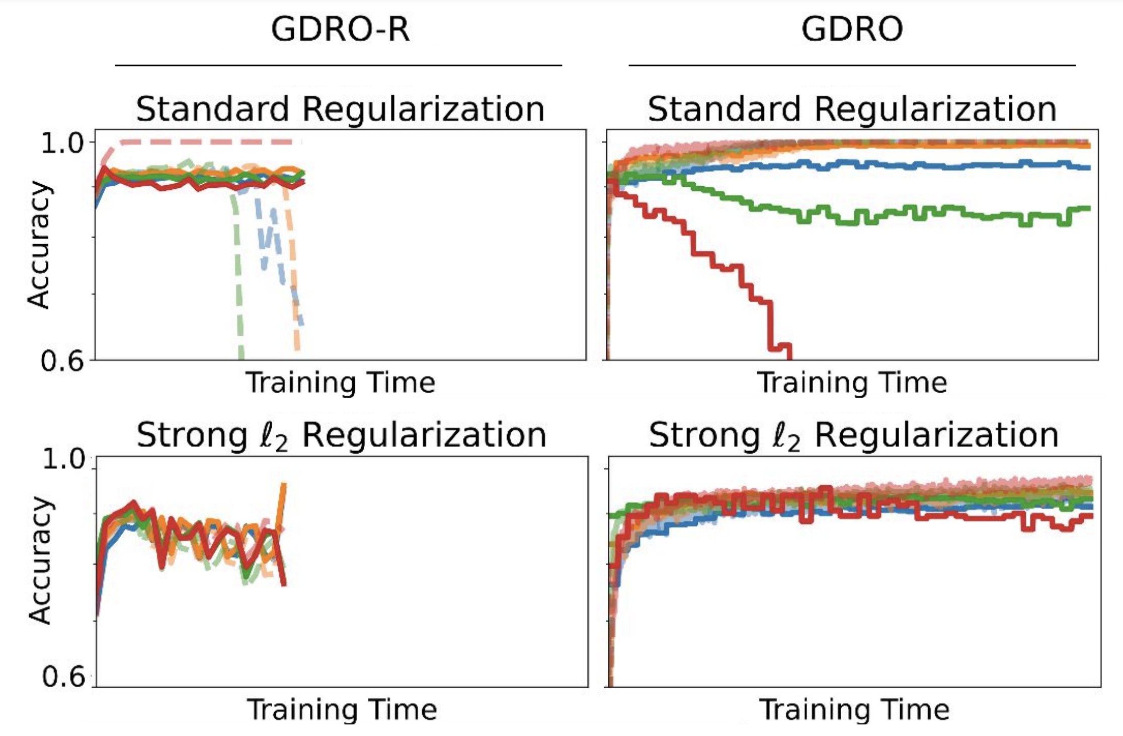
Figure 1: Training (light, dashed) and validation (dark, solid) accuracies for GDRO and R-MDL during training, plotted on a log scale. Note that R-MDL validation accuracy will be noisier than those of GDRO as we constrain R-MDL to limited samples (with replacement) from the validation set. In addition, in the left-most plot, training accuracy for all groups except the blond male group (red) dips to zero due to lack of data—this is because the blond male group (red) is the most challenging so the adversary eventually stops sampling from other groups. Under standard regularization, the red-group accuracy drops off in GDRO while R-MDL maintains a high red-group accuracy by heavily sampling from the red group, as reflected in the near-perfect red-group training error.

Datasets

Our experiments were performed on three datasets: Multi-NLI, CelebA, and Waterbirds [44]. We use identical preprocessing settings and dataset splits as Sagawa et al. [44]. Our experiments, unless otherwise specified, replicate the exact hyperparameter settings adopted by Sagawa et al. [44] for their Table 2 experiments. This includes the choice of random seeds, batch sizes, learning rates, learning schedules, and regularization. We defer readers to Sagawa et al. [44] or to our public source code for replication details.

The Multi-NLI dataset [51] concerns the following natural language inference task: determine if one statement is entailed by, neutral with, or contradicts a given statement. This dataset is challenging because traditional ERM models are prone to spuriously correlating “contradiction” labels with the existence of negation words. The dataset is divided into 6 distributions: the Cartesian product of the label space (entailment, neutral, contradiction) and an indicator of whether the sentence contains a negation word. The label space annotations were annotated by [51] while negation labels were annotated by Sagawa et al. [44]. There are 206,175 datapoints available in the Multi-NLI dataset; the smallest distribution (entailment + negation) is represented by only 1,521 datapoints. We use a randomly shuffled 50-20-30 training-validation-testing split.

The CelebA dataset is a dataset of celebrity face images and a label space of potential physical attributes [30]. This dataset is challenging because traditional ERM models are prone to spuriously correlating attribute labels with demographic information such as race and gender. Following Sagawa et al. [44], we divide the dataset into 4 distributions: the Cartesian product of the blond vs dark hair attribute label (“Blond_Hair”) with the “gender” attribute label (“Male”). Note that the authors of Liu et al. [30] limited the “gender” attribute label to binary options of male and not male. There are 162,770 datapoints available in the CelebA dataset; the smallest distribution (blond-hair + male) is represented by only 1,387 datapoints. We use the official training-testing-validation dataset split.

The Waterbirds dataset is a dataset by Sagawa et al. [44] curated from a larger Caltech-UCSD Birds-200-2011 (CUB) dataset [50]. It concerns the task of predicting whether a bird is of some waterbird (sub)species from an image of said bird. This dataset is challenging because traditional ERM models are prone to spuriously correlating backgrounds with foreground subjects; for instance, a model may often predict that a bird is a waterbird only because the image of the bird was taken at a beach. The dataset has 4 distributions: the Cartesian product of the waterbird vs not waterbird label with whether the background of the picture is over water. There are 4,795 datapoints available in the Waterbirds dataset; the smallest distribution (waterbirds on land) is represented by only 56 examples.

Models

We use two classes of models in our experiments: Resnet-50 [23] and BERT [16]. We use the torchvision [32] implementation of the convolutional neural network Resnet-50, with a default choice of a stochastic gradient descent optimizer with momentum 0.9 and batch size 128. Batch normalization is used; data augmentation and dropout are not used. We use the HuggingFace [52] implementation of the language model BERT, with a default choice of an Adam optimizer with dropout and batch size 32.

Hyperparameters

In the Standard Regularization experiments, we use a Resnet-50 model with an $\ell$-2 regularization parameter of $\lambda=0.0001$ and a fixed learning rate of $\alpha=0.001$ for both Waterbirds and CelebA datasets. The ERM and Group DRO baselines are trained on CelebA for 50 epochs and Waterbirds for 300 epochs. Our multi-distribution learning method is trained on CelebA for only 20 epochs and Waterbirds for 100 epochs; this is due to the faster training error convergence of our method. For the MultiNLI dataset, we use a BERT model with a linearly decaying learning rate starting at $\alpha_{0}=0.00002$ and no $\ell$-2 regularization. The ERM and Group DRO baselines are trained on Multi-NLI for 20 epochs. Our multi-distribution learning method is trained on Multi-NLI for only 10 epochs. Our multi-distribution learning method uses adversary learning rates $\eta_{\text{+}}$ of 1, 1, 0.2 on Waterbirds, CelebA and MultiNLI respectively.

In the Strong Regularization experiments, we follow similar settings to the Standard Regularization experiments. The only change is that an $\ell$-2 regularization parameter of $\lambda=1$ is used for Waterbirds and an $\ell$-2 regularization parameter of $\lambda=0.1$ is used for CelebA. Our multi-distribution learning method uses adversary learning rates $\eta_{\text{+}}$ of 1 and 0.2 on Waterbirds and CelebA respectively.

In the Early Stopping experiments, we follow similar settings to the Standard Regularization experiments. The only change is that all CelebA and Waterbird experiments are run for a single epoch. MultiNLI experiments are run for 3 epochs. Our multi-distribution learning method uses adversary learning rates $\eta_{\text{+}}$ of 1, 1, 1 on Waterbirds, CelebA and MultiNLI respectively.

The only hyperparameters we use that differ from prior literature are the number of training epochs and the adversary learning rates of our method (R-MDL). The choice of epoch was not fine-tuned, and was selected due to our observation of early training error convergence. We selected our adversary learning rate $\eta_{\text{-}}$ by training our method, on each dataset, for both $\eta_{\text{-}}=1$ and $\eta_{\text{-}}=0.2$ and selecting the $\eta_{\text{-}}$ yielding the highest validation-split worst-group accuracy.

Compute

The total amount of compute run for the experiments in this section is approximately 50 GPU hours. A “n1-standard-8” machine was leased from the Cloud computing service Google Cloud; the “n1-standard-8” machine was equipped with 8 Intel Broadwell chips and 1 NVIDIA Tesla V100 GPU. The cost of these computing resources totaled approximately USD $2 per hour, with a total cost of approximately USD $100. All results described in this section, with the exception of existing results cited from other works, were obtained with experiments on said machine. All experiments were implemented in Python and PyTorch.

References

• Alon et al. [2013] N. Alon, N. Cesa-Bianchi, C. Gentile, and Y. Mansour. From bandits to experts: a tale of domination and independence. In C. J. C. Burges, L. Bottou, Z. Ghahramani, and K. Q. Weinberger, editors, Advances in Neural Information Processing Systems 26, pages 1610–1618. Curran Associates, Inc., 2013.
• Alon et al. [2021] N. Alon, O. Ben-Eliezer, Y. Dagan, S. Moran, M. Naor, and E. Yogev. Adversarial laws of large numbers and optimal regret in online classification. In Proceedings of the Annual ACM SIGACT Symposium on Theory of Computing (STOC), volume 53, pages 447–455. ACM, 2021.
• Anthony and Bartlett [2002] M. Anthony and P. L. Bartlett. Neural Network Learning - Theoretical Foundations. Cambridge University Press, 2002. ISBN 978-0-521-57353-5.
• Balcan et al. [2012] M.-F. Balcan, A. Blum, S. Fine, and Y. Mansour. Distributed learning, communication complexity and privacy. In S. Mannor, N. Srebro, and R. C. Williamson, editors, Proceedings of the Conference on Learning Theory (COLT), volume 23 of Proceedings of Machine Learning Research, pages 26.1–26.22. PMLR, 2012.
• Beck and Teboulle [2003] A. Beck and M. Teboulle. Mirror descent and nonlinear projected subgradient methods for convex optimization. Operations Research Letters, 31(3):167–175, 2003.
• Ben-David and Schuller [2003] S. Ben-David and R. Schuller. Exploiting task relatedness for multiple task learning. In B. Schölkopf and M. K. Warmuth, editors, Learning Theory and Kernel Machines, pages 567–580. Springer Berlin Heidelberg, 2003.
• Ben-Tal et al. [2009] A. Ben-Tal, L. El Ghaoui, and A. Nemirovski. Robust Optimization, volume 28 of Princeton Series in Applied Mathematics. Princeton University Press, 2009.
• Blum et al. [2017] A. Blum, N. Haghtalab, A. D. Procaccia, and M. Qiao. Collaborative PAC learning. In I. Guyon, U. V. Luxburg, S. Bengio, H. Wallach, R. Fergus, S. Vishwanathan, and R. Garnett, editors, Advances in Neural Information Processing Systems 30, pages 2392–2401. Curran Associates, Inc., 2017.
• Blum et al. [2021a] A. Blum, N. Haghtalab, R. L. Phillips, and H. Shao. One for one, or all for all: equilibria and optimality of collaboration in federated learning. In M. Meila and T. Zhang, editors, Proceedings of the International Conference on Machine Learning (ICML), volume 139 of Proceedings of Machine Learning Research, pages 1005–1014. PMLR, 2021a.
• Blum et al. [2021b] A. Blum, S. Heinecke, and L. Reyzin. Communication-aware collaborative learning. In Proceedings of the AAAI Conference on Artificial Intelligence (AAAI), volume 35, pages 6786–6793. AAAI Press, 2021b.
• Boyd et al. [2011] S. Boyd, N. Parikh, E. Chu, B. Peleato, and J. Eckstein. Distributed optimization and statistical learning via the alternating direction method of multipliers. Foundations and Trends in Machine Learning, 3(1):1–122, Jan 2011.
• Chen et al. [2018] J. Chen, Q. Zhang, and Y. Zhou. Tight bounds for collaborative PAC learning via multiplicative weights. In S. Bengio, H. Wallach, H. Larochelle, K. Grauman, N. Cesa-Bianchi, and R. Garnett, editors, Advances in Neural Information Processing Systems 31, pages 3602–3611. Curran Associates, Inc., 2018.
• Daskalakis et al. [2011] C. Daskalakis, A. Deckelbaum, and A. Kim. Near-optimal no-regret algorithms for zero-sum games. In Proceedings of the Annual ACM-SIAM Symposium on Discrete Algorithms (SODA), volume 22, pages 235–254. SIAM, 2011.
• Daskalakis et al. [2021] C. Daskalakis, M. Fishelson, and N. Golowich. Near-optimal no-regret learning in general games. In M. Ranzato, A. Beygelzimer, Y. Dauphin, P. Liang, and J. W. Vaughan, editors, Advances in Neural Information Processing Systems 34, pages 27604–27616. Curran Associates, Inc., 2021.
• Daumé et al. [2012] H. Daumé, J. M. Phillips, A. Saha, and S. Venkatasubramanian. Efficient protocols for distributed classification and optimization. In Proceedings of the Algorithmic Learning Theory, volume 7568 of Lecture Notes in Computer Science, pages 154–168. Springer, 2012.
• Devlin et al. [2019] J. Devlin, M.-W. Chang, K. Lee, and K. Toutanova. BERT: pre-training of deep bidirectional transformers for language understanding. In Proceedings of the Conference of the North American Chapter of the Association for Computational Linguistics, pages 4171–4186. Association for Computational Linguistics, 2019.
• Duchi and Namkoong [2021] J. C. Duchi and H. Namkoong. Learning models with uniform performance via distributionally robust optimization. The Annals of Statistics, 49(3):1378 – 1406, 2021.
• Dwork et al. [2021] C. Dwork, M. P. Kim, O. Reingold, G. N. Rothblum, and G. Yona. Outcome indistinguishability. In Proceedings of the Annual ACM SIGACT Symposium on Theory of Computing (STOC), pages 1095–1108. ACM, 2021.
• Ehrenfeucht et al. [1989] A. Ehrenfeucht, D. Haussler, M. Kearns, and L. Valiant. A general lower bound on the number of examples needed for learning. Information and Computation, 82(3):247–261, 1989.
• Freund and Schapire [1997] Y. Freund and R. E. Schapire. A decision-theoretic generalization of on-line learning and an application to boosting. Journal of Computer and System Sciences, 55(1):119–139, 1997.
• Hart and Mas-Colell [2000] S. Hart and A. Mas-Colell. A simple adaptive procedure leading to correlated equilibrium. Econometrica, 68(5):1127–1150, 2000.
• Hashimoto et al. [2018] T. B. Hashimoto, M. Srivastava, H. Namkoong, and P. Liang. Fairness without demographics in repeated loss minimization. In J. Dy and A. Krause, editors, Proceedings of the International Conference on Machine Learning (ICML), volume 80 of Proceedings of Machine Learning Research, pages 1934–1943. PMLR, 2018.
• He et al. [2016] K. He, X. Zhang, S. Ren, and J. Sun. Deep residual learning for image recognition. In Proceedings of the IEEE Conference on Computer Vision and Pattern Recognition, pages 770–778. IEEE Computer Society, 2016.
• Hu et al. [2022] L. Hu, C. Peale, and O. Reingold. Metric entropy duality and the sample complexity of outcome indistinguishability. In Proceedings of the Algorithmic Learning Theory, volume 167 of Proceedings of Machine Learning Research, pages 515–552. PMLR, 2022.
• Kar et al. [2019] A. Kar, A. Prakash, M.-Y. Liu, E. Cameracci, J. Yuan, M. Rusiniak, D. Acuna, A. Torralba, and S. Fidler. Meta-Sim: learning to generate synthetic datasets. In Proceedings of the International Conference on Computer Vision, pages 4550–4559. IEEE, 2019.
• Karp and Kleinberg [2007] R. M. Karp and R. Kleinberg. Noisy binary search and its applications. In Proceedings of the Annual ACM-SIAM Symposium on Discrete Algorithms (SODA), pages 881–890. SIAM, 2007.
• Konečný et al. [2016a] J. Konečný, H. B. McMahan, D. Ramage, and P. Richtárik. Federated optimization: Distributed machine learning for on-device intelligence, 2016a.
• Konečný et al. [2016b] J. Konečný, H. B. McMahan, F. X. Yu, P. Richtárik, A. T. Suresh, and D. Bacon. Federated learning: strategies for improving communication efficiency, 2016b.
• Littlestone [1987] N. Littlestone. Learning quickly when irrelevant attributes abound: a new linear-threshold algorithm. Machine Learning, 2(4):285–318, 1987.
• Liu et al. [2015] Z. Liu, P. Luo, X. Wang, and X. Tang. Deep learning face attributes in the wild. In Proceedings of the International Conference on Computer Vision, pages 3730–3738. IEEE Computer Society, 2015.
• Mansour et al. [2008] Y. Mansour, M. Mohri, and A. Rostamizadeh. Domain Adaptation with Multiple Sources. In D. Koller, D. Schuurmans, Y. Bengio, and L. Bottou, editors, Advances in Neural Information Processing Systems 21, pages 1041–1048. Curran Associates, Inc., 2008.
• Marcel and Rodriguez [2010] S. Marcel and Y. Rodriguez. Torchvision the machine-vision package of torch. In Proceedings of the International Conference on Multimedia, pages 1485–1488. ACM, 2010.
• McMahan et al. [2017] B. McMahan, E. Moore, D. Ramage, S. Hampson, and B. A. y. Arcas. Communication-efficient learning of deep networks from decentralized data. In A. Singh and J. Zhu, editors, Proceedings of the International Conference on Artificial Intelligence and Statistics (AISTATS), volume 54 of Proceedings of Machine Learning Research, pages 1273–1282. PMLR, 2017.
• Mohri et al. [2019] M. Mohri, G. Sivek, and A. T. Suresh. Agnostic federated learning. In K. Chaudhuri and R. Salakhutdinov, editors, Proceedings of the International Conference on Machine Learning (ICML), volume 97 of Proceedings of Machine Learning Research, pages 4615–4625. PMLR, 2019.
• Nemirovskij and Yudin [1983] A. S. Nemirovskij and D. B. Yudin. Problem Complexity and Method Efficiency in Optimization. Wiley-Interscience, 1983.
• Neu [2015] G. Neu. Explore no more: Improved high-probability regret bounds for non-stochastic bandits. In C. Cortes, N. D. Lawrence, D. D. Lee, M. Sugiyama, and R. Garnett, editors, Advances in Neural Information Processing Systems 28, pages 3168–3176, 2015.
• Nguyen and Zakynthinou [2018] H. L. Nguyen and L. Zakynthinou. Improved algorithms for collaborative PAC learning. In S. Bengio, H. Wallach, H. Larochelle, K. Grauman, N. Cesa-Bianchi, and R. Garnett, editors, Advances in Neural Information Processing Systems 31, pages 7642–7650. Curran Associates, Inc., 2018.
• Rabbat and Nowak [2005] M. G. Rabbat and R. D. Nowak. Quantized incremental algorithms for distributed optimization. IEEE Journal on Selected Areas in Communications, 23(4):798–808, 2005.
• Rakhlin and Sridharan [2013] A. Rakhlin and K. Sridharan. Optimization, learning, and games with predictable sequences. In C. Burges, L. Bottou, M. Welling, Z. Ghahramani, and K. Weinberger, editors, Advances in Neural Information Processing Systems 26, pages 3066–3074, 2013.
• Ramaswamy et al. [2021] V. V. Ramaswamy, S. S. Kim, and O. Russakovsky. Fair attribute classification through latent space de-biasing. In Proceedings of the IEEE Conference on Computer Vision and Pattern Recognition, pages 9301–9310, 2021.
• Robbins and Monro [1951] H. Robbins and S. Monro. A stochastic approximation method. The Annals of Mathematical Statistics, pages 400–407, 1951.
• Robinson [1951] J. Robinson. An iterative method of solving a game. Annals of Mathematics, pages 296–301, 1951.
• Rothblum and Yona [2021] G. N. Rothblum and G. Yona. Multi-group agnostic PAC learnability. In M. Meila and T. Zhang, editors, Proceedings of the International Conference on Machine Learning (ICML), volume 139 of Proceedings of Machine Learning Research, pages 9107–9115. PMLR, 2021.
• Sagawa et al. [2020a] S. Sagawa, P. W. Koh, T. B. Hashimoto, and P. Liang. Distributionally robust neural networks. In Proceedings of the International Conference on Learning Representations (ICLR). OpenReview, 2020a.
• Sagawa et al. [2020b] S. Sagawa, A. Raghunathan, P. W. Koh, and P. Liang. An investigation of why overparameterization exacerbates spurious correlations. In H. Daumé III and A. Singh, editors, Proceedings of the International Conference on Machine Learning (ICML), volume 119 of Proceedings of Machine Learning Research, pages 8346–8356. PMLR, 2020b.
• Shamir et al. [2014] O. Shamir, N. Srebro, and T. Zhang. Communication-efficient distributed optimization using an approximate newton-type method. In E. P. Xing and T. Jebara, editors, Proceedings of the International Conference on Machine Learning (ICML), volume 32 of Proceedings of Machine Learning Research, pages 1000–1008. PMLR, 2014.
• Tosh and Hsu [2022] C. J. Tosh and D. Hsu. Simple and near-optimal algorithms for hidden stratification and multi-group learning. In K. Chaudhuri, S. Jegelka, L. Song, C. Szepesvari, G. Niu, and S. Sabato, editors, Proceedings of the International Conference on Machine Learning (ICML), volume 162 of Proceedings of Machine Learning Research, pages 21633–21657. PMLR, 2022.
• Valiant [1984] L. G. Valiant. A theory of the learnable. In Proceedings of the Annual ACM SIGACT Symposium on Theory of Computing (STOC), pages 436–445. ACM, 1984.
• Vishnoi [2021] N. K. Vishnoi. Algorithms for Convex Optimization. Cambridge University Press, 2021.
• Wah et al. [2011] C. Wah, S. Branson, P. Welinder, P. Perona, and S. Belongie. The Caltech-UCSD Birds-200-2011 dataset. Technical report, California Institute of Technology, 2011.
• Williams et al. [2018] A. Williams, N. Nangia, and S. Bowman. A broad-coverage challenge corpus for sentence understanding through inference. In Proceedings of the Conference of the North American Chapter of the Association for Computational Linguistics, pages 1112–1122. Association for Computational Linguistics, 2018.
• Wolf et al. [2019] T. Wolf, L. Debut, V. Sanh, J. Chaumond, C. Delangue, A. Moi, P. Cistac, T. Rault, R. Louf, M. Funtowicz, and others. Huggingface’s transformers: state-of-the-art natural language processing, 2019.
• Zakharov et al. [2019] S. Zakharov, W. Kehl, and S. Ilic. DeceptionNet: network-driven domain randomization. In Proceedings of the International Conference on Computer Vision, pages 532–541. IEEE, 2019.
• Zhang [2019] C. Zhang. Information-theoretic lower bounds of PAC sample complexity, 2019.
• Zhang et al. [2023] L. Zhang, P. Zhao, T. Yang, and Z. Zhou. Stochastic approximation approaches to group distributionally robust optimization, 2023.