H-SAUR: Hypothesize, Simulate, Act, Update, and Repeat
for Understanding Object Articulations from Interactions

Abstract

The world is filled with articulated objects that are difficult to determine how to use from vision alone, e.g., a door might open inwards or outwards. Humans handle these objects with strategic trial-and-error: first pushing a door then pulling if that doesn’t work. We enable these capabilities in autonomous agents by proposing “Hypothesize, Simulate, Act, Update, and Repeat” (H-SAUR), a probabilistic generative framework that simultaneously generates a distribution of hypotheses about how objects articulate given input observations, captures certainty over hypotheses over time, and infer plausible actions for exploration and goal-conditioned manipulation. We compare our model with existing work in manipulating objects after a handful of exploration actions, on the PartNet-Mobility dataset. We further propose a novel PuzzleBoxes benchmark that contains locked boxes that require multiple steps to solve. We show that the proposed model significantly outperforms the current state-of-the-art articulated object manipulation framework, despite using zero training data. We further improve the test-time efficiency of H-SAUR by integrating a learned prior from learning-based vision models.

I Introduction

Every day we are surrounded by a number of articulated objects that require specific interactions to use: our laptops can be opened or shut, windows can be raised or lowered, and drawers can be pulled out or pushed back in. A robot designed to function in real-world contexts should thus be able to understand and interact with these articulated objects.

Recent advances in deep reinforcement learning (RL) have focused on this problem and enabled robots to manipulate articulated objects such as drawers and doors [1, 2, 3, 4]. However, these systems typically produce fixed actions based on observations of a scene, and thus, when the articulated joint is ambiguous (e.g., a door that slides or swings), they cannot adapt their policies in response to failed actions. While some systems attempt to adjust policies during test-time exploration to recover from failure modes [5, 6], they only propose local action adjustments (pull harder or run faster) and so are insufficient in cases where dramatically different strategies need to be applied, e.g., from “sliding the window” to “pushing the window outward from the bottom.”

In contrast, humans and many other animals can quickly figure out how to manipulate complex articulated man-made objects, e.g., puzzle boxes, with very little training [7, 8, 9]. These capabilities are thought to be supported by rapid, strategic trial-and-error learning – interacting with objects in an intelligent way, but learning when actions lead to failures and updating mental representations of the world to reflect this information [10]. We argue that robotic systems that can learn how to manipulate articulated objects should be designed using similar principles.

In this work, we propose “Hypothesize, Simulate, Act, Update, and Repeat” (H-SAUR), an exploration strategy that allows an agent to figure out the underlying articulation mechanism of man-made objects from a handful of actions. At the core of our model is a probabilistic generative model that generates hypotheses of how articulated objects might deform given an action. Given a kinematic object, our model first generates several hypothetical articulation configurations of the object from 3D point clouds segmented by object parts. Our model then evaluates the likelihood of each hypothesis through analysis-by-synthesis – the proposed model simulates objects representative of each hypothetical configuration, using a physics engine to predict likely outcomes given an action. The virtual simulation helps resolve three critical components in this interactive perception setup: (1) deciding real-world exploratory actions that might produce meaningful outcomes, (2) reducing uncertainty over beliefs after observing the action-outcome pairs from real-world interactions, (3) generating actions that will lead to successful execution of a given task after fully figuring out the articulation mechanism. The contributions of this paper can be summarized as follows:

1. We propose a novel exploration algorithm for efficient exploration and manipulation of puzzle boxes and articulated objects, by integrating the power of probabilistic generative models and forward simulation. Our model explicitly captures the uncertainty over articulation hypotheses.

2. We compare H-SAUR against existing state-of-the-art methods, and show it outperforms them in operating unknown articulated object, despite requiring many fewer interactions with the object of interest.

3. We propose a new manipulation benchmark – PuzzleBoxes – which consists of locked boxes that require multi-step sequential actions to unlock and open, in order to test the ability to explore and manipulate complex articulated objects.

II Related Work

Kinematic Structure Estimation. A natural first step to manipulate an object is to predict the articulation mechanism of the object. Li et al. [11] and Wang et al. [12] proposed models to segment object point clouds into independently moving parts and articulated joints. However, this requires part and articulation annotations, and thus does not generalize to unexpected articulation mechanisms. Previous work address this by proposing to visually parse articulated objects under motion [13, 14, 15, 16, 17, 18]. Yet, most work assumes the objects are manually articulated by humans or scripted actions from the robot. In this paper, we study how an agent can jointly infer articulation mechanism and exploratory actions that helps to reveal the articulation of an object, i.e., in an interactive perception setup [19]. Niekum et al. [20] addresses a similar setup, but only handles articulated objects with a single joint and assumes the robot knows where to apply forces. Kulick et al. [21] and Baum et al. [22] handle dependency joints but assume each joint is either locked or unlocked, which is ambiguous for general kinematic objects. H-SAUR takes raw point clouds and part segmentations as inputs, and infers both the joint structure of the object and how to act. This model can handle articulated objects with an arbitrary number of joints and joint dependencies by leveraging off-the-shelf physics simulation for general physical constraint reasoning.

Model-free approaches for manipulating articulated objects. Instead of explicitly inferring the articulation mechanism, recent works in deep RL learn to generate plausible object manipulation actions from pointclouds [23, 3, 5], RGB-(D) images [4, 1, 2], or the full 3D state of the objects and their segments [24, 25, 26]. While most of these RL approaches learn through explicit rewards, recent approaches have learned to manipulate objects in a self-supervised manner, through self-driven goals or imitation learning [27, 28]. However, all of these systems require a large number of interactions during training and cannot discover hidden mechanisms that are only revealed through test-time exploratory behaviors. Furthermore, while they focus on training-time exploration, our work focuses on testing-time exploration where only a small number of interactions is permitted.

III Method

We consider a task of estimating kinematic structure of an unknown articulated object and use the estimation for efficient manipulation. We are particularly interested in manipulating a visually ambiguous object, e.g., a closed door that can be opened by pulling, pushing, sliding, etc. In such a situation, the agent needs to estimate its underlying kinematic configuration, and update its beliefs over different configurations based on the outcome of past failed actions.

We propose “Hypothesize, Simulate, Act, Update, and Repeat” (H-SAUR), a physics-aware generative model that represents an articulated object manipulation scene in terms of 3D shapes of object parts, articulation joint types and positions of each part, actions to apply on the object, and the change to the object after applying the actions. In this work, we assume to have access to a physics engine that can take as input 3D meshes (estimated from a point cloud) of a target unknown object with an estimated kinematic configuration, and produce hypothetical simulated articulations of this object when kinematically acted upon. The method consists of three parts. First, we initiate a number of hypothetical configurations that imitate a target object by sampling articulation structures from a prior distribution. The prior distribution can be uniform or from learned vision models. Second, we sample one of the hypotheses to generate an action that is expected to provide evidence for or against that hypothesis. Finally, we apply the optimal action to the target object and update beliefs about object joints based on the outcome.

III-A Generating Hypothetical Articulated Objects

Given the observed pointcloud $O$ of a target object along with its part segmentation, $m,$ we generate a number of kinematic replicas of the object. Since the true articulation mechanism is initially unknown, we generate these replicas by sampling different kinematic structures from uniform prior distributions over joint types and parameters.

Object Parts. From the observed pointcloud $O$ and segmentation masks, $m_{1},m_{2},\cdots,m_{N_{v}},$ where $N_{v}$ is number of available views, we can break the pointcloud into part-centric pointcloud $O^{1},O^{2},\cdots,O^{N_{p}}$ where $N_{p}$ is the total number of object parts.

Articulation Joints. Each object part is attached to a base of the object with a joint. We consider three most common types of articulation joints: revolute (r), prismatic (p), and fixed (f). For revolute and prismatic joints, we further generate possible joint axes and positions, using the tight bounding boxes fitted to the part-centric pointcloud to obtain a total of ${J}$ possible joints. The $j^{\text{th}}$ joint is denoted as $\theta^{(j)}=(c,d)$ where $c\in\{r,p,f\}$ is the joint type and $d\in\mathbb{R}^{6}$ is the 6-DoF pose of the joint axis. The prior distribution $p(\theta^{(j)})$ for the joint type is assumed to be uniform at $t=0.$ One can also use learned prior from vision models that predict joint types.

In addition, most articulated joints have lower and upper limits of how much the joint can be deformed. We denote the limits as $\theta^{\text{low}}$ and $\theta^{\text{high}}.$ The prior distribution is sampled uniformly from $[-\theta_{\text{MAX}},0]$ and $[0,\theta_{\text{MAX}}],$ respectively. The full state of the joint for object part $O^{i}$ is $s^{i}=(\theta^{(\sigma(i))},\theta^{\text{low}_{i}},\theta^{\text{high}_{i}},\theta^{\text{cur}_{i}})$, where $\sigma(i)\in\{1,2,\cdots,J\}$ is the joint configuration for the $i^{\text{th}}$ object part, and $\theta^{\text{cur}_{i}}$ is the joint position at the current time step. The prior over all the latent variables is:

$$p(s^{1:N_{p}})=\prod_{i=1}^{N_{p}}p(\theta^{(\sigma(i))})p_{\text{unif}[-\theta_{\text{MAX}},0]}(\theta^{\text{low}_{i}})p_{\text{unif}[0,\theta_{\text{MAX}}]}(\theta^{\text{high}_{i}}).$$ (1)

We approximate the distribution by maintaining a particle pool, $\mathcal{S},$ where each particle in the pool represents a particular setup for the articulation configurations.

III-B Simulating and Selecting Informative Action

We utilize virtual simulations to generate an optimal action that reduces the uncertainty of joint configuration hypotheses. Yet, computing the optimal action that maximizes the information gain involves integral over all latent variables, which is intractable. One can approximate this by a sampling-based method [19]. However, the high computational requirements still prohibit the agent from solving the task within a reasonable time. We address this by using only a single particle to make a noisy approximation of the optimal action.

We sample a joint configuration from the set of particles $s^{(k)}\sim\mathcal{S}$ and obtain the optimal action by simulating different actions on the object with the physics simulation. The action $a_{t}=(p,r)\in\mathbb{R}^{6}$ is represented as a 3D point $p_{t}\in\mathbb{R}^{3}$ on the object and the direction $r_{t}\in\mathbb{R}^{3}$ to apply force. The optimal action is defined as the action that can maximally deform the object or a target object part over a single step. For multi-part objects, we maintain a list of parts-of-interest, which we will introduce shortly, and we sample a target part from the list to act on. We measure how much an object part $i$ deforms by $d_{i}=\|\theta_{t+1}^{\text{cur}_{i}}-\theta_{t}^{\text{cur}_{i}}\|.$ Although one can naively sample a huge number of actions and pick the best action through simulation, we found this can be extremely inefficient with large object parts. To improve inference speed, we instead treat the action inference as a particle filtering problem: we initialize a number of action proposals by randomly sampling 3D locations on the target point cloud and assign random directions to apply force, then we use the measured distance $d_{j}$ as the likelihood to update the posterior distribution of the particles. We add noise to the action while reproducing the particles from previous iterations. We continue this process three times and finally sample a particle from the pool to obtain the action $a^{\ast}$. We found the inferred action $a^{\ast}$ is often close to the oracle optimal action that maximizes $d_{i}$.

The probabilistic formulation of an articulation mechanism given past observation and action is

$$\begin{split}p(s_{t}|O_{1:t-1}&,a_{1:t-1})\\ &=\int\underbrace{p(s_{t}|s_{t-1},a_{t-1})}_{\text{forward dynamics}}\underbrace{p(s_{t-1}|O_{1:t-1},a_{1:t-1})}_{\text{obtain through recursion}},\end{split}$$ (2)

where the first term is handled by the physics engine by forward simulation, and the second is initialized with the prior defined in Eq. (1) and can be obtained through recursion.

III-C Updating hypotheses through analysis-by-synthesis

We apply the inferred action $a^{\ast}$ on the target object $O_{t}$ to observe outcome $O_{t+1}$. We then update the probability of each hypothesis through analysis-by-synthesis: we first apply the same action $a^{\ast}$ on all the "imagined" objects, $s\in\mathcal{S}$ in the physics engine. After applying the action, we obtain $\hat{O}^{(k)}_{t+1}$ for each particle $s^{(k)}.$ We define the likelihood of the particle $s^{(k)}$ as $w_{k}=\frac{1}{\text{dist}(O_{t+1},\hat{O}^{(k)}_{t+1})+\epsilon}$, where $\text{dist}(o_{1},o_{2})=\frac{1}{|o_{1}|}\sum_{x\in o_{1}}\min_{y\in o_{2}}\|x-y\|_{2}^{2}$ is the chamfer distance between two point cloud $o_{1}$ and $o_{2}.$ The overall updated posterior is:

$$\begin{split}p(s_{t}|O_{1:t},a_{1:t-1})&\propto p(O_{t}|s_{t})p(s_{t}|O_{1:t-1},a_{1:t-1})\\ &=\sum_{k=1}^{K}w_{k}p(s_{t}|O_{1:t-1},a_{1:t-1}),\end{split}$$ (3)

where the second term can be computed from Eq.(2), and the whole inference is implemented through particle filtering with weighted sampling.

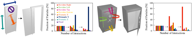
Figure 2: Percentage of particles representing different hypothetical configurations during interactions. The hypotheses start as a uniform distribution, then with an observed action, belief tends to aggregate on the correct joint type.

		Novel instances in training Categories						Testing categories
		Box	Door	Microwave	Fridge	Cabinet	Mean	Safe	Table	Washing	Mean
Closed	PN2	$\mathbf{100.0}$	$43.3$	$97.4$	$72.9$	$69.2$	$76.5$	$55.7$	$56.5$	$45.2$	$54.0$
	Ours	$\mathbf{100.0}$	$\mathbf{85.4}$	$\mathbf{100.0}$	$\mathbf{98.6}$	$96.7$	$\mathbf{96.1}$	$89.7$	$98.7$	$\mathbf{100.0}$	$96.1$
	PN2+Ours	$\mathbf{100.0}$	$80.5$	$90.9$	$\mathbf{98.6}$	$\mathbf{97.7}$	$93.4$	$\mathbf{96.6}$	$\mathbf{99.3}$	$93.8$	$\mathbf{96.5}$
Half-opened	PN2	$\mathbf{100.0}$	$87.5$	$\mathbf{100.0}$	$99.1$	$\mathbf{99.8}$	$\mathbf{97.4}$	$\mathbf{100.0}$	$92.2$	$77.4$	$89.9$
	Ours	$\mathbf{100.0}$	$\mathbf{97.6}$	$81.8$	$\mathbf{100.0}$	$99.0$	$95.7$	$\mathbf{100.0}$	$92.8$	$\mathbf{100.0}$	$\mathbf{97.6}$
	PN2+Ours	$92.3$	$90.2$	$\mathbf{100.0}$	$98.6$	$98.6$	$96.0$	$\mathbf{100.0}$	$\mathbf{93.4}$	$93.8$	$95.7$

TABLE I: Joint type estimation accuracy [%].

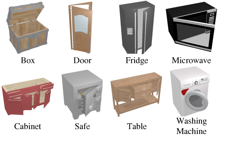
Figure 3: Categories from PartNet-Mobility dataset used for our experiments.

III-D Handling Joints with Dependency in Goal-Conditioned Manipulation

A real puzzle box often consists of joints with dependencies, e.g., a lock needs to be open first in order to operate on another lock. Randomly selecting a part to act on is ineffective and may not be sufficient to solve the problem since (1) the agent can act on a segment that is irrelevant to the task, e.g., a decoration on the box, and (2) the agent can underestimate the joint limit by ignoring the possibility that another part is blocking the current joint. To resolve this issue, we propose to keep track of the relevant parts and gradually grow a dependency tree throughout the exploration process.

Given goals in the form of “moving part X towards Y”, we maintain a parts-of-interest list $q_{\text{POI}}$ to keep track of task-relevant object parts and their desired position. For example, consider a door with a few locks, whose goal is to pull open the door. Thus, we initialize $q_{\text{POI}}$ by adding the “door” part, $O_{0}$, and the desirable moving direction $d_{0}$. When selecting an action (see section III-B), we always act on the most recently added object part. In the first run, we select the door since it is the only part in the list.

Using the physics engine, we not only infer the optimal action that would cause desirable changes to the target part, but also detect object parts, e.g., locks on the PuzzleBoxes we introduce shortly, that will collide with it. We consider these collided parts as having a dependency with target part at hand. We can further infer the desirable change direction $d_{i}$ for each of these collided parts $O_{i}$ that would unblock the current part. Then, we add the part along with the desired changing direction to $q_{\text{POI}}.$ Sometimes multiple directions might lead to a successful unblock, in this case, we randomly select one direction to be put in the list. We expect the pool of particles to keep track of different sampling outcomes. We can keep adding “unsolved” parts with dependencies to the current parts to the list. A part is marked as “solved” and removed from the list if it can be and has been changed to a desired configuration that unblocks its parent node in the dependency tree.

	Novel instances in training categories						Testing categories
Method	Box	Door	Microwave	Fridge	Cabinet	Mean	Safe	Table	Washing	Mean
Binary classification accuracy [%] $\uparrow$
W2A ($10$K)	$68.6$	$59.7$	$70.6$	$70.1$	$69.7$	$67.7$	$68.5$	$63.9$	$60.3$	$64.2$
W2A ($100$K)	$75.9$	$60.2$	$81.1$	$71.3$	$70.0$	$71.7$	$74.1$	$53.5$	$66.1$	$64.6$
Ours ($0.01$K)	$\mathbf{96.4}$	$\mathbf{79.5}$	$\mathbf{97.8}$	$\mathbf{93.0}$	$\mathbf{93.0}$	$\mathbf{91.9}$	$\mathbf{93.3}$	$\mathbf{97.4}$	$\mathbf{91.3}$	$\mathbf{94.0}$
Distance prediction error $\downarrow$
W2A ($10$K)	$0.051$	$0.074$	$0.040$	$0.068$	$0.062$	$0.059$	$0.057$	$0.053$	$0.076$	$0.062$
W2A ($100$K)	$0.049$	$0.072$	$0.032$	$0.063$	$0.057$	$0.055$	$\mathbf{0.051}$	$0.061$	$0.067$	$0.059$
Ours ($0.01$K)	$\mathbf{0.009}$	$\mathbf{0.036}$	$\mathbf{0.013}$	$\mathbf{0.040}$	$\mathbf{0.026}$	$\mathbf{0.025}$	$0.055$	$\mathbf{0.016}$	$\mathbf{0.029}$	$\mathbf{0.033}$

TABLE II: Affordance prediction performance.

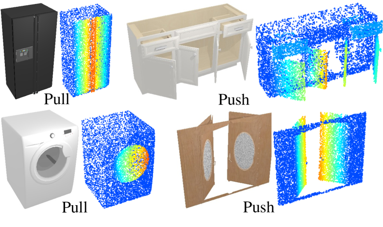
Figure 4: Visualizations of distance prediction. The warmer color shows larger deformations.

IV Experiments

We evaluate H-SAUR on both the PartNet-Mobility dataset and PuzzleBoxes dataset on SAPIEN [29] physics engine.

The PartNet-Mobility dataset provides a wide variety of synthetic articulated objects. We specifically use $8$ different categories as shown in Fig. 3 with two different settings: In the closed setting, all movable joints are shut, which is often the most visually ambiguous setup for an object. In the half-opened setting, all joints are initialized at the midway point between the joint limits.

The PuzzleBoxes dataset has more challenging configurations and joint dependency. Inspired by the puzzle box experiment by Thorndike [7], we manually design PuzzleBoxes with different levels with different number of locks ($N^{\text{locks}}$) and dependency chains ($N^{\text{chain}}$). As shown in Fig. 5, we prepared five different settings: $(N^{\text{chain}},N^{\text{locks}})\sim\{(1,1),(2,1),(3,1),(1,2),(1,3)\}$, where each setting has 10 different configurations (joint type, axis, and position).

In both dataset, the 6-DoF action is implemented in the simulator by simulating a directed force on a 3D point, imitating actions from a suction gripper.

IV-A Joint type estimation

We first evaluate how well H-SAUR can estimate the type, location, and limits of joints on an articulated object.

Settings. We test joint estimation using the PartNet-Mobility dataset with both the closed and half-opened settings. To measure the performance, we cast the problem into an eight-way classification problem where the model classifies the target joint as one of the followings: four different revolute joints attached to the right, left, top, or bottom of the 3D bounding boxes for the object part, three different prismatic joints that moves along each of the X, Y, and Z axes, or a fixed joint (see Fig. 2).

Models. We initialize a uniform prior for H-SAUR  with the eight possible joints, using $110$ particles. The algorithm stops if one of the following conditions is satisfied: (1) the model has good confidence with more than $90\%$ of the particles belong to a single class, or (2) the model interacts with the object $10$ times. We compare our algorithm to a supervised learning baseline PN2 [11], which uses PointNet++ [30] as a feature extraction backbone to predict joint types given an input point cloud and segmentation masks of the object parts connected to the joint. We train the model to classify the link as one of the eight joint types described above. We also test the combination of H-SAUR and PointNet++, which we denote Ours + PN2, where we use the trained PointNet++ model as a prior when initializing particles.

Results and analysis. Table I shows the joint type estimation accuracy. Our model performs comparably with PN2 in the half-opened setting and significantly outperform PN2 on the closed setting where joint type is mostly ambiguous from vision alone. We also show, by integrating visual prior from PN2 with the proposed framework, we can improve in cases where visual prior helps significantly, e.g., in half-opened Microwave. We visualize the posterior over hypotheses in Fig. 2. We can see our model becomes more confident after a few interactions.

IV-B Joint type estimation under stochastic dynamics.

Settings. We further evaluate the performance of H-SAUR under stochastic dynamics by adding noise to action to imitate a stochastic dynamics. The action noise $\epsilon$ is uniformly sampled from $\bm{\epsilon}\sim[-\sigma,\sigma]^{6}$ thus the action on the stochastic dynamics will be $a^{\text{noise}}_{t}=a_{t}+\bm{\epsilon}$. We evaluate H-SAUR with $\sigma\in\{0,0.1,0.2,0.3\}$, where $\sigma=0$ corresponds to Ours in Table I.

Results and analysis. Table III shows the results on different noise levels. At its most extreme, the noise is sampled from a uniform range of width $0.6$ meters, which is the equivalent to the size of the articulated part in many cases, yet adding this noise has little effect on joint estimation performance. This is partly because our method is a probabilistic framework, thus it can handle any uncertainty including stochastic dynamics, part segmentation, action noises, etc.

$\sigma$	Box	Door	Microwave	Fridge	Cabinet	Safe	Table	Washing	Mean
$0.0$	$\mathbf{100.0}$	$85.4$	$\mathbf{100.0}$	$\mathbf{98.6}$	$96.7$	$89.7$	$\mathbf{98.7}$	$\mathbf{100.0}$	$\mathbf{96.1}$
$0.1$	$96.1$	$\mathbf{94.8}$	$\mathbf{100.0}$	$87.8$	$90.9$	$\mathbf{95.9}$	$96.6$	$87.5$	$93.6$
$0.2$	$95.4$	$92.8$	$\mathbf{100.0}$	$82.9$	$\mathbf{100.0}$	$\mathbf{95.9}$	$82.8$	$87.5$	$92.2$
$0.3$	$95.2$	$92.8$	$\mathbf{100.0}$	$85.4$	$\mathbf{100.0}$	$93.2$	$96.6$	$93.8$	$94.6$

TABLE III: Joint type estimation accuracy on noisy dynamics [%].

	Novel instances in training categories						Testing categories
	Box	Door	Microwave	Fridge	Cabinet	Mean	Safe	Table	Washing	Mean
W2A ($100$K)	$65.0$	$47.3$	$49.6$	$50.7$	$54.8$	$53.5$	$42.6$	$43.9$	$70.0$	52.2
W2A+HP ($100$K)	$\mathbf{96.2}$	$51.3$	$91.0$	$\mathbf{98.4}$	$92.9$	$85.9$	$72.8$	$72.0$	$94.3$	79.7
Ours ($0.01$K)	$83.9$	$\mathbf{90.2}$	$99.0$	$94.8$	$95.6$	$92.7$	$82.8$	$98.0$	$93.8$	$91.5$
Ours + PN2	$87.2$	$86.0$	$\mathbf{100.0}$	$94.7$	$\mathbf{97.1}$	$\mathbf{93.0}$	$\mathbf{85.6}$	$\mathbf{99.0}$	$\mathbf{97.7}$	$\mathbf{94.1}$

TABLE IV: The proportion of the part opened [%] with fifteen testing-time interactions.

Setting	1-chain	2-chain	3-chain	1-chain	1-chain
				2-locks	3-locks
Random	$23.3$	$6.7$	$0.0$	$13.3$	$3.3$
Heuristic	$36.7$	$13.3$	$0.0$	$23.3$	$10.0$
CURL	$33.3$	$0.0$	$0.0$	$0.0$	$0.0$
Ours	$\mathbf{96.7}$	$\mathbf{86.7}$	$\mathbf{80.0}$	$\mathbf{93.3}$	$\mathbf{86.7}$

TABLE V: Manipulation performance ($\%$) for solving PuzzleBoxes averaged from 3 runs.

IV-C Action Proposal and Affordance Map

We next measure how well the H-SAUR model can use its estimates of joint properties to estimate whether an action will be effective on the PartNet-Mobility dataset.

Settings. To evaluate all models, we collect $10,000$ interactions on the closed setting by randomly sampling a point belonging on a movable part and applying a force with a uniformly distributed direction on the surface of the 3-d unit sphere. An action is labeled as "success" if it causes the joint to move more than 5% of its full range. We counterbalance "success" and "failure" interactions in the final test set. We use two metrics to evaluate the models: (1) Binary classification Accuracy which is the proportion of actions correctly predicted as success or failure, and (2) Distance Prediction which measure the $\ell_{1}$ distance between the predicted point translation and the ground truth.

Baseline. We compare our model with the state-of-the-art articulated object manipulation algorithm, Where2Act (W2A) [23], which takes the pointcloud of an articulated object as input to predict an effectiveness score for all points. To train the model, we collect $\{10\text{K},100\text{K}\}$ number of counter-balanced interactions using the same procedure as above. For a fair comparison, we collect both the testing and training data from only movable links by applying a segmentation mask when sampling the position to interact as our method assumes segmentation of the parts is given.

Results and analysis. We show the results in Table II. Our method significantly outperforms the baseline, despite being $1000$ times more sample efficient. We show qualitative results of distance prediction by H-SAUR in Fig. 4.

IV-D Manipulation

Next we evaluate the estimated joints for manipulation task on the PartNet-Mobility Dataset.

Settings. The task is to open the movable parts as much as possible from completely closed setting within $N^{\text{max}}=15$ interactions. Our method uses first $N^{\text{int}}=10$ interactions to estimate the joint type, and the rest to manipulate the object while the baseline models use all $N^{\text{max}}$ interactions to open the movable parts. For evaluation, we measure the proportion of the part opened $r=\max_{t\in\{1,...,N^{\text{max}}\}}(\theta_{i}-\theta^{\text{init}})/(\theta^{\text{max}}-\theta^{\text{init}})$, where $r=1$ means fully opened target part.

Baselines. We again use Where2Act as the baseline for this experiment. We also add Where2Act + HP, which employs an additional heuristic that filters out actions that has a larger than 90 deg angle with last-step action as done in [4]. This heuristic helps to avoid sequences of back-and-forth actions.

Results and analysis. Table V shows our method significantly outperforms Where2Act in all categories and performs better than Where2Act+HP in most settings except for boxes and fridge. We found these two categories are simpler in the sense that all boxes open in the same direction (upward), and so do the fridges (to the left), so it is easy for Where2Act to overfit to a single action. We can also see that the performance of our method, when combined with the learned PN2 model, slightly improves. It shows H-SAUR  alone is already robust to skewed prior, and one can easily improve its performance by incorporating good prior from vision models.

IV-E PuzzleBoxes

Finally, we evaluate H-SAUR on a novel benchmark PuzzleBoxes. The task is to open a door outward more than $60^{\circ}$ within $100$ interactions. However, opening this door requires first moving other “locks” that restrict the door’s range of motion as shown in Fig. 5.

Baselines. To the best of our knowledge, none of the prior learning-based approaches can solve this long-term manipulation problem without exhaustively interacting with the objects before deployment time. To show this, we train an RL agent with CURL [31], a state-of-the-art image-based RL algorithm. We feed the model with RGBD images as inputs and train the agent with 10K interactions. We also compare our algorithm to two learning-free baselines: (1) Random: a policy that uniformly sample a movable link and apply randomly sampled action on it at each time step, (2) Heuristic: a policy that selects an action in the same way as Random, but keeps applying the same action if the object moves at the previous step.

Results and analysis. We show the results in Table V. We can see that the RL baseline trained with 10K timesteps, which corresponds to 100x more timesteps than ours, performs poorly on all but the simplest levels. Deep RL algorithms generally needs enormous amount of interactions to learn, and can fail drastically when the agent is allowed to have a limited number of interactions. Aside from poor sample efficiency, most learning-based policies would generate similar actions (drawn from a fixed distribution) given similar observations (as PuzzleBoxes are designed to look similar but have different joint axes), since most policies only take one or a few past observations as inputs and do not update action distributions from past failed interactions. Even baselines that use knowledge of the problem structure (both Random and Heuristic) perform poorly on all levels. In contrast, H-SAUR can solve even the most complex levels far above chance.

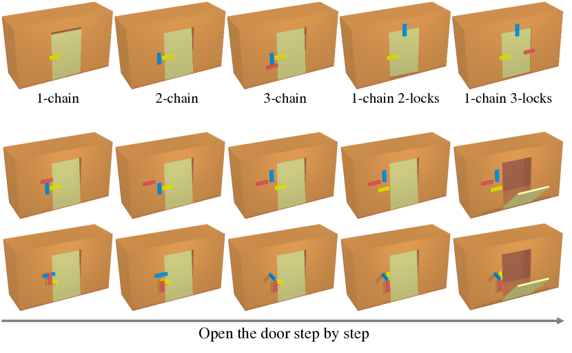
Figure 5: Top Examples from the PuzzleBoxes Benchmark. Bottom Visualizations of how the puzzle boxes will be opened by unlocking keys in 3-chain puzzle boxes.

V Conclusion

In this work, we propose a physics- and uncertainty-aware exploration framework, H-SAUR, that can manipulate diverse articulated objects in circumstances where visual inputs do not uniquely specify the state. We show H-SAUR can open complex puzzle boxes requiring several steps to solve. We also show the proposed model outperforms baselines by a large margin, highlighting the importance of quick behavior adaption through test-time exploration. Our model operates directly on pointcloud segments without the needs of detailed tracking using AR tags or any other tracking system, which increases its chance to transfer to a real-world setup. Current results show the model is robust to mismatch between the object of interest and the reconstructed virtual objects from the pointcloud segments.

We note that more work is needed to extend H-SAUR to manipulate arbitrary real-world articulated objects. First, our current model cannot handle articulated joints with arbitrary joint axis, e.g., a door that rotates with a tilted joint, or joint types that have not been prespecified in its hypothesis space. This problem can potentially be addressed using motion-based kinematic prediction [13] to propose new hypothesis to include in the prior. Second, we assume part segments are given. In ongoing work, we are investigating models that jointly infers object parts and their articulations. Third, we assume a force can be applied to any point on an object from any direction in order to separate reasoning about joints from manipulating them. While this is roughly similar to using a suction gripper as in [4, 32], we plan to explore practical constraints imposed by a real robot’s geometry, gripper, etc. in future work.

Nonetheless, H-SAUR demonstrates a promising avenue for systems that can reason about articulated objects, manipulate them, and update beliefs in real time.

-A Additional Results

-A1 Ablation on different scoring methods to update hypotheses.

In this section, we compare two different scoring functions for updating hypotheses: chamfer distance as used in our method (described in Sec. III-C), and cosine similarity referring [33]. The cosine similarity $\beta_{k}$ measures the cosine of the angle between the displacement of the real object $\bm{d}$ and the displacement of a hypothetical object. The direction $\bm{d}$ is computed by $\bm{d}_{t}=\bm{p}_{t+1}-\bm{p}_{t}$, where $\bm{p}_{t}$ is the center position of the observed point cloud $O^{j}_{t}$ as $\bm{p}_{t}=\frac{1}{\|O_{t}\|}\sum_{\bm{x}\in O^{j}_{t}}\bm{x}$. The cosine similarity is computed by using the direction as $\beta_{k}=\arccos\left(\frac{\bm{d}_{t}\cdot\hat{\bm{d}}^{(k)}_{t}}{|\bm{d}_{t}||\hat{\bm{d}}^{(k)}_{t}|}\right)$. We then use $\beta_{k}$ for the likelihood of the $k$-th particle $s^{(k)}$ as $w_{k}=(\beta_{k}+1)/2$. This formulation results in an increase of the likelihood when a hypothetical object successfully imitates the movement of the real object. Following [33], we assign $w_{k}=1$ when both objects do not move, and $w_{k}=0$ in the case of only one of the two objects moves, where we assume such situation can happen when the hypothetical configuration is wrong. To wrap up, cosine similarity-based likelihood function can be formulated as:

$$w_{k}=\begin{cases}(\beta_{k}+1)/2&\text{if $\bm{d}_{t}\neq\bm{0}$ and $\hat{\bm{d}}^{(k)}_{t}\neq\bm{0}$}\\ 1&\text{if $\bm{d}_{t}=\bm{0}$ and $\hat{\bm{d}}^{(k)}_{t}=\bm{0}$}\\ 0&\text{otherwise}.\end{cases}$$ (4)

Table VI shows the comparison of the two different scoring functions to update hypotheses for joint type estimation experiments. It clearly shows that chamfer distance outperforms the cosine similarity. We found that cosine similarity works poorly especially when the joint state of the real object is close to the upper or lower limit. In such situations, only either hypothetical or real object moves and results in $w_{k}=0$, and filtered out from the particle pool. Chamfer distance, however, is robust to the wrong joint state or joint upper/lower limit, because it still returns a reasonable value even if the estimated state or joint limits is wrong.

		Box	Door	Microwave	Fridge	Cabinet	Safe	Table	Washing	Mean
Closed	Chamfer distance	$\mathbf{100.0}$	$\mathbf{85.4}$	$\mathbf{100.0}$	$\mathbf{98.6}$	$\mathbf{96.7}$	$\mathbf{89.7}$	$\mathbf{98.7}$	$\mathbf{100.0}$	$\mathbf{96.1}$
	Cosine similarity	$78.4$	$83.0$	$69.2$	$73.2$	$72.7$	$73.5$	$74.0$	$82.8$	$76.0$

TABLE VI: Comparison of different scoring methods to update hypotheses for joint type estimation accuracy [%].

-B Implementation Details

-B1 Joint Proposals from Part Segments

Given an object part segment from the point cloud, our method initializes a set of 19 joint proposals from the tight axis-oriented minimum bounding box of the part segment. Figure 6 illustrates the joint proposals from a bounding box. The 19 joint proposals have their joint positions lie either on the surfaces of the tight bounding box or at the center of the box, and have their joint axes aligned to the X, Y, or Z-axis of the box. Specifically, for revolute joints, we assume the joint lies at the center of one of the 6 surfaces on the box, with 3 possible axes directions aligned with the box, result in $15$ different joint positions ($15=3\times 6-3$ as there are $3$ duplicate joint positions for each axis). For prismatic joint, we assume the joint lies at the center of the box and can move along 3 axes direction of the box. We found these joint proposals can cover well most articulated objects in the real world.

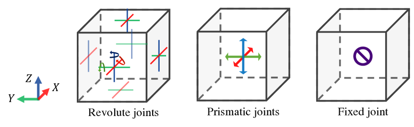
Figure 6: Visualizations of how to define joint positions for the revolute, prismatic, and fixed joints. On the left, you can see X, Y, or Z-axis revolute joints (shown by red, green, and blue colors) are attached to each surface of the axis-aligned bounding box. On the middle, we show the prismatic joints that move the hypothetical object towards X, Y, or Z-axis direction from its observed position. Finally, the fixed joint on the right does not change position or orientation of the hypothetical object.

-B2 Dataset and Simulation Details

PartNet-Mobility Dataset Detailed instance statistics and their joint types for each object category are listed in Table VII.

Training Categories							Test Categories
Category	Instances		Joints		Rev.	Pris.	Category	Instances	Joints	Rev.	Pris.
	Train	Test	Train	Test
Box	10	3	10	3	X	-	Safe	29	29	X	-
Door	26	7	33	8	X	-	Table	62	153	X	X
Microwave	8	3	8	3	X	-	Washing	16	16	X	-
Fridge	34	9	56	17	X	-
Cabinet	269	68	630	157	X	X
All	347	90	737	188	X	X	All	107	198	X	X

TABLE VII: Statistics of the data splits.

For physics simulation setups, we use frame rate $100$ fps, and all the other settings as default in SAPIEN release. When interacting with an object, we apply the same force for $10$ simulation steps, resulting in $10$ fps simulation. To simulate actions from position control, we set the magnitude of the force by multiplying $100\times m$, where $m$ is the mass of the target part. Following Where2Act [23], we disable collision simulation between every pair of two parts connected by an articulated joint. We also set gravity to zero to better simulate articulated objects that have an opener that needs to be opened upwards, e.g., Boxes. Setting gravity to zero prevents the opener to gradually fall back from open to close without any force applied.

For the rendering settings, we use four cameras to get pointcloud of the target object. We set the near plane to $0.1$, far plane to $100$, resolution to $640\times 480$, and field of view to $35^{\circ}$. We obtain a pointcloud from the depth images by back-projecting the depth image into pointclouds, removing the far-away (background) points, and down-sampling the point to get a total of $10$K points.

For the object parts, we remove parts that are either too small or has function irrelevant to physical articulation. For example, some instances in the Washing Machine category have tiny buttons for controlling the machines. We ignore these parts and focus on articulated parts, such as doors.

PuzzleBox We aim to create a more comprehensive version of Thorndike’s puzzle box experiment [7], where a cat needs to escape a cage by exploring a locked door and finally opening it. We design the boxes with different level of difficulties by varying the number of locks and the number of decency. We show boxes with different levels in Fig. 7.

In the 1-chain N-locks setups, the door is blocked by a number of sliding locks and revolving locks. To solve the task, an agent needs to figure out which locks are blocking the door and how to manipulate these locks to resolve the blocking dependency. In these 1-chain setups, we assume the locks can be solved independently. To further test whether an agent can optimally explore by only researching on task decency locks, we also include boxes with dummy locks, e.g., locks that are already open and are not blocking the doors.

In the 2-chain and 3-chain setups, we test whether an agent can solve a chain of locks with dependency, i.e., the locks need to be operated in a specific order to fully unlock the door. In Fig. 8, we show some example design of the locks.

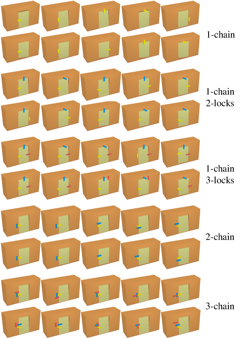
Figure 7: All instances from the PuzzleBoxes Benchmark.

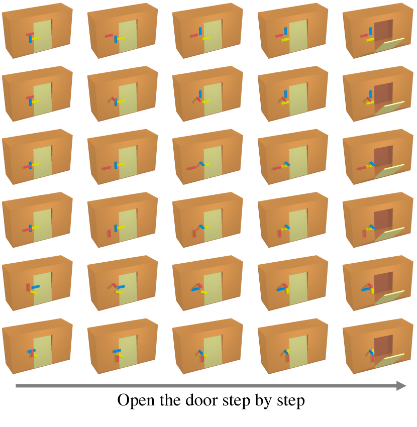
Figure 8: Visualizations of how the puzzle boxes will be opened by unlocking keys in 3-chain puzzle boxes.

-C Implementation Details in the Joint Type Estimation Experiment

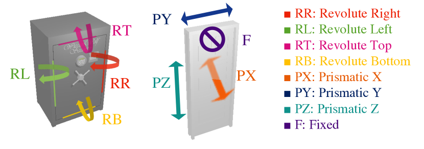
Figure 9: Joint configurations used for PartNet-Mobility dataset.

Types of Joints Considered To measure the performance, we cast the problem into an eight-way classification problem where the model classifies the target joint as one of the followings: (4) revolute joints attached to the right, left, top, or bottom of the 3D bounding boxes for the object part, (3) prismatic joints that moves along each of the X, Y, and Z axes, and a fixed joint. We illustrates the joints in Fig. 9.

PN2 Following [23], we use PointNet++ network [30] and implementation [34] as a backbone feature extractor with four set abstraction layers with single-scale grouping for the encoder and four feature propagation layers for the decoder. We feed the extracted feature into a classification network which consists of two $256$-dim fully connected layers and 8-dim fully connected layer that classifies the input into the 8 possible joints.

PN2+Ours We can initialize the hypothesis distribution of the proposed model with prediction from PN2. However, we found that PN2 can generates almost zero weight on a correct hypothesis when it becomes over-confident about a false configuration. This can cause the proposed model to fail since all the particles are initialized with the over-weighted false configuration. To handle the problem, we impose a minimum weight $1/16$ on all the hypotheses to ensure all hypotheses are covered in the particle pool. We found the heuristic can significantly improve the overall performance (from $80.5\%$ to $96.5\%$ on closed setting with test categories).

-C1 Implementation Details in the RL Experiment for PuzzleBoxes

This section provides more detailed implementation settings about the RL experiment described in Sec. IV-E.

-C2 Environment

State

For a fair comparison to H-SAUR, which requires part segments and 3D information as point cloud, we define the state of the environment is two frames of RGBD image $I^{RGBD}\in\mathbb{R}^{100\times 100\times 8}$. The RGB image corresponds to part segments because all parts in PuzzleBoxes have unique color (see Fig. 7), and the depth image gives the 3D information to an RL agent.

Action

The action of the agent consists of an interaction position and direction. The position is defined by 2D continuous value $a^{\text{pos}}\in[-1,1]^{2}$, and we find the closest pixel in the RGBD image and then find the corresponding 3D position to the pixel. This enables to make the action space smaller, and makes the RL agent easier to solve the task. The interaction direction is defined by 3D continuous values $a^{\text{dir}}\in[-1,1]^{3}$, and normalized so that it will be a unit vector.

Rewards

Since training an RL agent entirely from a sparse reward is too hard to solve, we define a shaped reward to enhance exploration, which consists of changes in position of any joint $r^{\text{shape}}=\|\bm{\theta}_{t+1}-\bm{\theta}_{t}\|$, where $\bm{\theta}$ is a joint state vector that consists of all movable joints.

Terminal conditions

An episode terminates with the same condition with other methods as described in Sec. IV-E: an agent opens the door outward for more than $60^{\circ}$, or the total step of an episode is over $100$.

-C3 Agent

We used CURL [31], which uses contrastive learning to acquire a good image representation, for our RL experiments with the same hyper parameters used in the original paper.

-C4 Training

We used a random policy to collect $1$K transitions to a replay buffer before training an RL agent, and then trained the RL agent for $10$K timesteps. The configurations of PuzzleBoxes for train and test are different: we use $7$ configurations for training and $3$ configurations for testing, and we train RL agents for each PuzzleBoxes type separately.

Appendix A Pseudo Code for H-SAUR

Here we provide pseudo code for the proposed method in Algorithm 1, 2, 3, and 4. Specifically, Algorithm 3, 4 handles joints with dependency, as described in Section 3.4. Since objects in the PartNet-Mobility Dataset do not have such dependency, they can be solved with Algorithm 1, 2 without the dependency check (highlighted in red in Algorithm 1). For objects in the PuzzleBox dataset, including the dependency check is critical to achieve reasonable performance.

Algorithm 1 Interactive Joint Type Estimation

Input Observed point cloud for the current movable part $O^{i}$, hypothetical joint configurations $\bm{\theta}=\{\theta^{(j)}|j\in\{1,2,\cdots,J\}\}$, number of particles $N^{\text{particles}}$, threshold $\delta^{\text{prob}}$ to finish estimation, maximum steps to interact with the real-world object $N^{\text{max}}$
      Output Estimated joint type $j^{\ast}$ and indexes of the collided movable parts $k$

1:Initialize a particle pool $\mathcal{S}^{\text{state}}=\emptyset$

2:for $k\leftarrow 1$ to $N^{\text{particles}}$ do

3:     Sample a joint configuration $\theta^{(\sigma(k))}\sim p_{0}(\bm{\theta})$ $\triangleright$ Can use a learned prior distribution

4:     Sample a joint upper limit $\theta^{\text{high}_{k}}\sim p_{\text{unif}[0,\theta_{\text{MAX}}]}$

5:     Sample a joint lower limit $\theta^{\text{low}_{k}}\sim p_{\text{unif}[-\theta_{\text{MAX}},0]}$

6:     Add the sampled particle $s^{k}=(\theta^{(\sigma(k))},\theta^{\text{low}_{k}},\theta^{\text{high}_{k}},\theta^{\text{cur}_{k}}=0)$ to the particle pool $\mathcal{S}^{\text{state}}\leftarrow\mathcal{S}^{\text{state}}\cup s^{k}$

7:end for

8:for $t\leftarrow 1$ to $N^{\text{max}}$ do

9:     Infer an informative action $a^{\ast}$ using Alg. 2

10:     Apply the inferred action $a^{\ast}$ on the real-world object and observe the pointcloud $O_{t+1}$

11:     // Handling movable parts/joints with dependency

12:     if Detect contacts between the current movable part and other movable parts then

13:         Break the current loop

14:     end if

15:     for all $k\leftarrow 1$ to $N^{\text{particles}}$ do

16:         Apply the inferred action $a^{\ast}$ on $k$-th hypothetical object and observe the pointcloud $\hat{O}_{t+1}^{k}$

17:         Compute importance weight for the particle $w_{k}=\frac{1}{\text{dist}(O_{t+1},\hat{O}^{k}_{t+1})+\epsilon}$

18:     end for

19:     Re-sample particles from $\mathcal{S}^{\text{state}}$ according to the importance weights. Compute updated posterior $p_{t+1}(\bm{\theta})$ from the particles.

20:     if $\max_{j\in\{1,...,J\}}p_{t+1}(\theta^{(j)})>\delta^{\text{prob}}$ then

21:         Break the current loop

22:     end if

23:end for

24:return The most probable joint configuration $j^{\ast}=\mathop{\rm arg~{}max}\limits_{j\in\{1,...,J\}}p(\theta^{(j)})$ and indexes of the collided movable part $k$

Algorithm 2 Informative Action Selection

Input Observed point cloud for the current movable part $O_{i}$, particle pool $\mathcal{S}^{\text{state}}$, number of particles for generating action $N^{\text{particles-action}}$, number of particle updates $N^{\text{update}}$
      Output Informative action $a^{\ast}$

1:Sample a joint configuration $s\sim\mathcal{S}^{\text{state}}$

2:Reproduce a hypothetical object using the joint configuration $s$ in a physics engine

3:Initialize a particle pool $\mathcal{S}^{\text{action}}=\emptyset$

4:for $k\leftarrow 1$ to $N^{\text{particles-action}}$ do

5:     Sample a point to interact $p_{k}\sim O_{i}$

6:     Sample a force direction $r_{k}\sim\text{\{+x,-x, +y, -y, +z, -z\}}$

7:     Add the sampled particle $a_{k}=(p_{k},r_{k})$ to the particle pool $\mathcal{S}^{\text{action}}\leftarrow\mathcal{S}^{\text{action}}\cup a_{k}$

8:end for

9:for $n\leftarrow 1$ to $N^{\text{update}}$ do

10:     for $k\leftarrow 1$ to $N^{\text{particles-action}}$ do

11:         Apply the sampled action $a_{k}$ on the hypothetical object and observe the joint state $\theta_{t+1,k}^{s}$

12:         Compute importance weight for the particle $w_{k}=\|\theta_{t+1,k}^{s}-\theta_{t,k}^{s}\|$

13:     end for

14:     Re-sample particles from $\mathcal{S}^{\text{action}}$ according to the importance weights

15:     Add noise to the position $p_{k}\in\mathcal{S}^{\text{action}}$

16:end for

17:return The most probable particle $a^{\ast}=a_{k^{\ast}}$, where $k^{\ast}=\mathop{\rm arg~{}max}\limits_{k\in\{1,...,N^{\text{particles-action}}\}}w_{k}$

Algorithm 3 Unlock PuzzleBoxes

Input Pointcloud of the target object $O,$ segmentation masks $m_{1},m_{2},\cdots,m_{N_{v}},$ target part ID $t$ to open, desired direction $d^{t}$ to displace the target part
      Output “Success” or “Failure” to solve the task

1:Obtain segmented point clouds $O_{1},O_{2},\cdots,O_{N_{v}}$ from $O$ and $m_{1},m_{2},\cdots,m_{N_{v}}$

2:Initialize the part-of-interest queue with the target part, e.g., the door, and its desired opening direction $q_{\text{POI}}=\{(O^{t},d^{t})\}$

3:while $|q_{\text{POI}}|\geq 0$ do

4:     Get the most recently added object part and its moving direction $(O^{l},d^{l})$ from the queue $q_{\text{POI}}$

5:     Estimate the joint type of the target part $O^{l}$ using Alg. 1

6:     if Detect collided parts during joint type estimation then

7:         Add the collided part $O^{k}$ and its unknown moving direction $d^{k}$ to the last of the part-of-interest list $q_{\text{POI}}\leftarrow q_{\text{POI}}\cup\{(O^{k},d^{k})\}$

8:     else

9:         if The moving direction $d^{l}$ is “unknown” then

10:              Compute the moving direction $d^{l}$ that resolves collision using Alg. 4

11:         end if

12:         Infer an optimal action $a^{\ast}$ on the estimated joint type using Alg. 2 while replacing the cost function $w_{k}=\|\theta_{t+1,k}^{s}-d^{l}\|$ in line.12 in Alg. 2 and apply it on the real-world object

13:         if Goal is achieved (e.g., “door is open”) then

14:              Terminate this experiment with “Success”

15:         else if Number of interactions exceeds $N^{\text{max-int}}$ then

16:              Terminate this experiment with “Failure”

17:         else if part $O^{l}$ has been successfully displaced with $d^{l}$ then

18:              Remove the current part and direction $q_{\text{POI}}\leftarrow q_{\text{POI}}\backslash\{(O^{l},d^{l})\}$

19:         end if

20:     end if

21:end while

22:return “Failure”

Algorithm 4 Compute Action Direction to Resolve Collision

Input Pointcloud of the current part of interest $O^{l}$, pointcloud of the collided object part $O^{\text{c}}$, estimated current part’s joint configuration $s=\{\theta^{\text{low}},\theta^{\text{high}},\theta^{l}\}$, number of samples to search for the desired joint state $N$
      Output Desired joint state $\theta^{\ast}$ for the collided object part

1:Reproduce a hypothetical object using the joint configuration $s$ in a physics engine.

2:Obtain pointclouds $\{O^{l}_{\theta_{1}},...,O^{l}_{\theta_{N}}\}$ of different joint states $\theta\in\{\theta_{1},...,\theta_{N}\}$ by setting the joint configuration $s$ with joint position $\theta$ in a physics engine, where $\theta$ is evenly spaced between $\theta^{\text{low}}$ and $\theta^{\text{high}}$.

3:return The joint state $\theta^{\ast}=\mathop{\rm arg~{}max}\limits_{\theta\in\{\theta_{1},...,\theta_{N}\}}\text{dist}(O^{l}_{\theta}$, $O^{\text{c}})$

References

- [1] S. Gu, E. Holly, T. P. Lillicrap, and S. Levine, “Deep reinforcement learning for robotic manipulation,” CoRR, vol. abs/1610.00633, 2016. [Online]. Available: http://arxiv.org/abs/1610.00633
- [2] Y. Urakami, A. Hodgkinson, C. Carlin, R. Leu, L. Rigazio, and P. Abbeel, “Doorgym: A scalable door opening environment and baseline agent,” CoRR, vol. abs/1908.01887, 2019. [Online]. Available: http://arxiv.org/abs/1908.01887
- [3] R. Wu, Y. Zhao, K. Mo, Z. Guo, Y. Wang, T. Wu, Q. Fan, X. Chen, L. Guibas, and H. Dong, “VAT-Mart: Learning visual action trajectory proposals for manipulating 3d articulated objects,” in International Conference on Learning Representations (ICLR), 2022.
- [4] Z. Xu, Z. He, and S. Song, “Universal manipulation policy network for articulated objects,” IEEE Robotics and Automation Letters, vol. 7, no. 2, pp. 2447–2454, 2022.
- [5] Y. Wang, R. Wu, K. Mo, J. Ke, Q. Fan, L. Guibas, and H. Dong, “AdaAfford: Learning to adapt manipulation affordance for 3d articulated objects via few-shot interactions,” 2021.
- [6] C. Finn, P. Abbeel, and S. Levine, “Model-agnostic meta-learning for fast adaptation of deep networks,” CoRR, vol. abs/1703.03400, 2017. [Online]. Available: http://arxiv.org/abs/1703.03400
- [7] E. L. Thorndike, “Animal intelligence,” Psych Revmonog, vol. 8, no. 2, pp. 207–208, 1911.
- [8] A. M. I. Auersperg, A. Kacelnik, and A. M. P. von Bayern, “Explorative learning and functional inferences on a five-step means-means-end problem in goffin’s cockatoos ( cacatua goffini ),” PLoS ONE, vol. 8, 2013.
- [9] E. S. Bridge, K. Thorup, M. S. Bowlin, P. B. Chilson, R. H. Diehl, R. W. Fléron, P. Hartl, R. Kays, J. F. Kelly, W. D. Robinson, and M. Wikelski, “Technology on the Move: Recent and Forthcoming Innovations for Tracking Migratory Birds,” BioScience, vol. 61, no. 9, pp. 689–698, 09 2011. [Online]. Available: https://doi.org/10.1525/bio.2011.61.9.7
- [10] K. R. Allen, K. A. Smith, and J. B. Tenenbaum, “Rapid trial-and-error learning with simulation supports flexible tool use and physical reasoning,” Proceedings of the National Academy of Sciences, vol. 117, no. 47, pp. 29 302–29 310, 2020.
- [11] X. Li, H. Wang, L. Yi, L. J. Guibas, A. L. Abbott, and S. Song, “Category-level articulated object pose estimation,” CoRR, vol. abs/1912.11913, 2019. [Online]. Available: http://arxiv.org/abs/1912.11913
- [12] X. Wang, B. Zhou, Y. Shi, X. Chen, Q. Zhao, and K. Xu, “Shape2motion: Joint analysis of motion parts and attributes from 3d shapes,” CoRR, vol. abs/1903.03911, 2019. [Online]. Available: http://arxiv.org/abs/1903.03911
- [13] Z. Jiang, C.-C. Hsu, and Y. Zhu, “Ditto: Building digital twins of articulated objects from interaction.” [Online]. Available: https://arxiv.org/abs/2202.08227
- [14] J. Sturm, C. Stachniss, and W. Burgard, “A probabilistic framework for learning kinematic models of articulated objects,” Journal of Artificial Intelligence Research, vol. 41, pp. 477–526, 2011.
- [15] N. Heppert, T. Migimatsu, B. Yi, C. Chen, and J. Bohg, “Category-independent articulated object tracking with factor graphs,” 2022. [Online]. Available: https://arxiv.org/abs/2205.03721
- [16] D. Katz, M. Kazemi, J. A. D. Bagnell, and A. T. Stentz, “Interactive segmentation, tracking, and kinematic modeling of unknown 3d articulated objects,” in Proceedings of (ICRA) International Conference on Robotics and Automation, May 2013, pp. 5003 – 5010.
- [17] T. Zhou and B. E. Shi, “Simultaneous learning of the structure and kinematic model of an articulated body from point clouds,” in 2016 International Joint Conference on Neural Networks (IJCNN), 2016, pp. 5248–5255.
- [18] C. G. Cifuentes, J. Issac, M. Wüthrich, S. Schaal, and J. Bohg, “Probabilistic articulated real-time tracking for robot manipulation,” CoRR, vol. abs/1610.04871, 2016. [Online]. Available: http://arxiv.org/abs/1610.04871
- [19] J. Bohg, K. Hausman, B. Sankaran, O. Brock, D. Kragic, S. Schaal, and G. S. Sukhatme, “Interactive perception: Leveraging action in perception and perception in action,” CoRR, vol. abs/1604.03670, 2016. [Online]. Available: http://arxiv.org/abs/1604.03670
- [20] K. Hausman, S. Niekum, S. Osentoski, and G. Sukhatme, “Active articulation model estimation through interactive perception,” in IEEE International Conference on Robotics and Automation, 2015.
- [21] M. Baum, M. Bernstein, R. Martin-Martin, S. Höfer, J. Kulick, M. Toussaint, A. Kacelnik, and O. Brock, “Opening a lockbox through physical exploration,” 11 2017, pp. 461–467.
- [22] ——, “Opening a lockbox through physical exploration,” in 2017 IEEE-RAS 17th International Conference on Humanoid Robotics (Humanoids), 2017, pp. 461–467.
- [23] K. Mo, L. J. Guibas, M. Mukadam, A. Gupta, and S. Tulsiani, “Where2act: From pixels to actions for articulated 3d objects,” in Proceedings of International Conference on Computer Vision (ICCV), October 2021, pp. 6813–6823.
- [24] T. Yu, D. Quillen, Z. He, R. Julian, K. Hausman, C. Finn, and S. Levine, “Meta-world: A benchmark and evaluation for multi-task and meta reinforcement learning,” CoRR, vol. abs/1910.10897, 2019. [Online]. Available: http://arxiv.org/abs/1910.10897
- [25] A. Ajay, A. Kumar, P. Agrawal, S. Levine, and O. Nachum, “OPAL: offline primitive discovery for accelerating offline reinforcement learning,” CoRR, vol. abs/2010.13611, 2020. [Online]. Available: https://arxiv.org/abs/2010.13611
- [26] K. Pertsch, Y. Lee, Y. Wu, and J. J. Lim, “Demonstration-guided reinforcement learning with learned skills,” 5th Conference on Robot Learning, 2021.
- [27] C. Lynch, M. Khansari, T. Xiao, V. Kumar, J. Tompson, S. Levine, and P. Sermanet, “Learning latent plans from play,” Conference on Robot Learning (CoRL), 2019. [Online]. Available: https://arxiv.org/abs/1903.01973
- [28] R. Dinyari, P. Sermanet, and C. Lynch, “Learning to play by imitating humans,” arXiv preprint arXiv:2006.06874, 2020.
- [29] F. Xiang, Y. Qin, K. Mo, Y. Xia, H. Zhu, F. Liu, M. Liu, H. Jiang, Y. Yuan, H. Wang, L. Yi, A. X. Chang, L. J. Guibas, and H. Su, “Sapien: A simulated part-based interactive environment,” in Proceedings of IEEE Conference on Computer Vision and Pattern Recognition (CVPR), 2020, pp. 11 094–11 104.
- [30] C. R. Qi, L. Yi, H. Su, and L. J. Guibas, “Pointnet++: Deep hierarchical feature learning on point sets in a metric space,” in Advances in Neural Information Processing Systems, 2017, pp. 5099–5108.
- [31] M. Laskin, A. Srinivas, and P. Abbeel, “CURL: Contrastive unsupervised representations for reinforcement learning,” in Proceedings of the 37th International Conference on Machine Learning, ser. Proceedings of Machine Learning Research, H. D. III and A. Singh, Eds., vol. 119. PMLR, 13–18 Jul 2020, pp. 5639–5650. [Online]. Available: https://proceedings.mlr.press/v119/laskin20a.html
- [32] A. Zeng, P. Florence, J. Tompson, S. Welker, J. Chien, M. Attarian, T. Armstrong, I. Krasin, D. Duong, V. Sindhwani, and J. Lee, “Transporter networks: Rearranging the visual world for robotic manipulation,” Conference on Robot Learning (CoRL), 2020.
- [33] K. Hausman, S. Niekum, S. Osentoski, and G. S. Sukhatme, “Active articulation model estimation through interactive perception,” in 2015 IEEE International Conference on Robotics and Automation (ICRA), 2015, pp. 3305–3312.
- [34] E. Wijmans, “Pointnet++ pytorch,” https://github.com/erikwijmans/Pointnet2_PyTorch, 2018.