Probing Transfer in Deep Reinforcement Learning without Task Engineering

Abstract

We evaluate the use of original game curricula supported by the Atari 2600 console as a heterogeneous transfer benchmark for deep reinforcement learning agents. Game designers created curricula using combinations of several discrete modifications to the basic versions of games such as Space Invaders, Breakout and Freeway, making them progressively more challenging for human players. By formally organising these modifications into several factors of variation, we are able to show that Analyses of Variance (ANOVA) are a potent tool for studying the effects of human-relevant domain changes on the learning and transfer performance of a deep reinforcement learning agent. Since no manual task engineering is needed on our part, leveraging the original multi-factorial design avoids the pitfalls of unintentionally biasing the experimental setup. We find that game design factors have a large and statistically significant impact on an agent’s ability to learn, and so do their combinatorial interactions. Furthermore, we show that zero-shot transfer from the basic games to their respective variations is possible, but the variance in performance is also largely explained by interactions between factors. As such, we argue that Atari game curricula offer a challenging benchmark for transfer learning in RL, that can help the community better understand the generalisation capabilities of RL agents along dimensions which meaningfully impact human generalisation performance. As a start, we report that value-function finetuning of regularly trained agents achieves positive transfer in a majority of cases, but significant headroom for algorithmic innovation remains. We conclude with the observation that selective transfer from multiple variants could further improve performance.

1 Introduction

A key open challenge in artificial intelligence is training reinforcement learning (RL) agents which generally achieve high returns when faced with critical changes to their environments (Schaul et al., 2018), motivated by impressive flexibility of animal and human learning. One way to approach the problem is through the prism of generalisation across related but distinct environments, also called transfer learning (Pan & Yang, 2009; Taylor & Stone, 2009) and comprehensively reviewed in the RL setting by Zhu et al. (2020). Many purpose-built benchmarks serve investigations into more specific research questions, e.g. transfer learning in particular cases where additional assumptions hold. While useful for progress, the challenge of transfer learning in the more general case remains.

Motivated by visual observation similarity, Machado et al. (2018) suggest using the newest iteration of the Atari Learning Environment (ALE) (Bellemare et al., 2013) to study the transfer learning between single-player game variants, or “flavours”, found in the curricula of many Atari game titles. We will use the terms default or basic game interchangeably to refer to the environment recommended by respective manuals as the entry point. We call all other distinct games variations or variants of their respective default game. Hence, each Atari game title we consider provides a curriculum consisting of a default and its variants, all designed to teach and challenge human players in novel ways.

Studying transfer within curricula ensures that environments are related, and that meaningful knowledge reuse should be possible and beneficial. Interestingly, differences in game variant dynamics, subtle changes in observations which are crucial for optimal behaviour, novel environment states, as well as new player abilities challenge unified approaches to transfer learning across variations. Farebrother et al. (2018) argue that Deep Q-Network (DQN) agents (Mnih et al., 2015), trained with appropriate regularisation, can be effective in zero-shot and finetuning transfer scenarios. In this work we study the learning and transfer performance of an updated version of the DQN agent, called Rainbow-IQN (Toromanoff et al., 2019). We use ANOVA to quantitatively confirm the suspected link between game design factors and agent performance. While current approaches occasionally achieve meaningful transfer from default games, they have limited success for variations with several modifications. Our analyses reveal this is due to strong interaction effects between factors, not just the isolated effects of the modifications they introduce. This reinforces the case for agents leveraging these systematic curricula, originally designed for human players, through transfer learning.

Contributions: (1) We show that discrete changes to Atari game environments, challenging for human players, also modulate the performance of a popular model-free deep reinforcement learning algorithm starting from scratch (2) Zero-shot transfer of policies trained on one game variation and tested on others can be significant, but performance is far from uniform across respective environments (3) Interestingly, zero-shot transfer variance from default game experts is also well explained by game design factors, especially their interactions (4) We empirically evaluate the performance of value-function finetuning, a general transfer learning technique compatible with model-free deep RL, and confirm that it can lead to positive transfer from basic game experts (5) We point out that more complex challenges of transfer with deep RL are captured by Atari game variations, e.g. appropriate source task selection, fast policy transfer and evaluation using experts, as well as data efficient behaviour adaptation more generally .

2 Background

Reinforcement Learning. A Markov Decision Processes (MDP) (Puterman, 1994) is the classic abstraction used to characterise the sequential interaction loop between an action taking agent and its environment, which responds with observations and rewards (Sutton & Barto, 2018). Formally, a finite MDP is a tuple $\mathcal{M}=\langle\mathcal{X},\mathcal{A},\mathcal{T},\mathcal{R},\gamma\rangle$, where $\mathcal{X}$ is the state space, $\mathcal{A}$ is the action space, both finite sets, $\mathcal{T}:\mathcal{X}\times\mathcal{A}\times\mathcal{X}\mapsto\left[0,1\right]$ is the stochastic transition function which maps each state and action to a probability distribution over possible future states $\mathcal{T}(x,a,x^{\prime})=P(x^{\prime}|x,a)$, $\mathcal{R}:\mathcal{X}\times\mathcal{A}\times\mathcal{X}\mapsto\mathbb{R}$ is the reward distribution function, with $r:\mathcal{X}\times\mathcal{A}\mapsto\mathbb{R}$ the expected immediate reward $r(x,a)=\mathbb{E}_{\mathcal{T}}\left[\mathcal{R}(x,a,x^{\prime})\right]$, and $\gamma\in[0,1]$ is the discount factor (Bellman, 1957). A stochastic policy function is the action selection strategy $\pi:\mathcal{X}\times\mathcal{A}\mapsto\left[0,1\right]$ which maps states to probability distributions over actions $\pi(x)=P(a|x)$. The discounted sum of future rewards is the random variable $Z_{\mathcal{M}}^{\pi}(x,a)=\sum_{t=0}^{\infty}\gamma^{t}r(x_{t},a_{t})$, where $x_{0}=x$, $a_{0}=a$, $x_{t}\sim\mathcal{T}(\cdot|x_{t-1},a_{t-1})$ and $a_{t}\sim\pi(\cdot|x_{t})$. Given an MDP $\mathcal{M}$ and a policy $\pi$, the value function is the expectation over the discounted sum of future rewards, also called the expected return: $V_{\mathcal{M}}^{\pi}(x)=\mathbb{E}\left[Z_{\mathcal{M}}^{\pi}(x,\pi(x))\right]$. The goal of Reinforcement Learning (RL) is to find a policy $\pi_{\mathcal{M}}^{*}:\mathcal{X}\mapsto\mathcal{A}$ which is optimal, in the sense that it maximises expected return in $\mathcal{M}$. The state-action Q-function is defined as $Q_{\mathcal{M}}^{\pi}(x,a)=\mathbb{E}\left[Z_{\mathcal{M}}^{\pi}(x,a)\right]$ and it satisfies the Bellman equation $Q_{\mathcal{M}}^{\pi}(x,a)=\mathbb{E}_{\mathcal{T}}\left[\mathcal{R}(x,a,x^{\prime})\right]+\gamma\mathbb{E}_{\mathcal{T},\pi}\left[Q_{\mathcal{M}}^{\pi}(x^{\prime},a^{\prime})\right]$ for all states $x\in\mathcal{X}$ and actions $a\in\mathcal{A}$. Mnih et al. (2013) adapted a reinforcement learning algorithm called Q-Learning (Watkins, 1989) to train deep neural networks end-to-end, mastering several Atari 2600 games, with inputs consisting of high-dimensional observations, in the form of console screen pixels, and differences in game scores. For more details please consult Appendix A.

Note that value functions depend critically on all aspects of the MDP. For any policy $\pi$, in general $Q_{\mathcal{M}}^{\pi}\neq Q_{\mathcal{M}^{\prime}}^{\pi}$ for MDPs $\mathcal{M}$ and $\mathcal{M}^{\prime}$ defined over the same state and action sets, with $\mathcal{T}\neq\mathcal{T}^{\prime}$ or $\mathcal{R}\neq\mathcal{R}^{\prime}$. Even if differences in dynamics or rewards are isolated to a subset of $\mathcal{X}\times\mathcal{A}$, changes may be induced across the support of $Q_{\mathcal{M}^{\prime}}^{\pi}$, since value functions are expectations over sums of discounted future rewards, issued according to $\mathcal{R}^{\prime}$, along sequences of states decided entirely by the new environment dynamics $\mathcal{T}^{\prime}$ when following a fixed behaviour policy $\pi$. Nevertheless, many particular cases of interest exist, which we discuss below.

Transfer learning. Described and motivated in its general form by Caruana (1997); Thrun & Pratt (1998); Bengio (2012), the goal of transfer learning is to use knowledge acquired from one or more source tasks to improve the learning process, or its outcomes, for one or more target tasks, e.g. by using fewer resources compared to learning from scratch. When this is achieved, we call it positive transfer. We often further qualify transfer learning by the metric used to measure specific effects. Several transfer learning metrics have been defined for the RL setting (Taylor & Stone, 2009), but none capture all aspects of interest on their own. A first metric we use is “jumpstart” or “zero-shot” transfer, which is performance on the target task before gaining access to its data. Another highly relevant metric is “performance with fixed training epochs” (Zhu et al., 2020), defined as returns achieved in the target task after using fixed computation and data budgets under transfer learning conditions.

One way to classify such approaches in RL is by the format of knowledge being transferred (Zhu et al., 2020), commonly: datasets, predictions, and/or parameters of neural networks encoding representations of observations, policies, value-functions or approximate state-transition “world models” acquired using source tasks. Another way to classify transfer learning approaches in RL is by their respective sets of assumptions about source and target tasks, also well illustrated by their associated benchmark domains: (1) Differences are limited to observations, but the underlying MDP is the same, e.g. domain adaptation and randomisation (Tobin et al., 2017), mastered through the generalisation abilities of large models (Cobbe et al., 2019; 2020) (2) MDP states and dynamics are the same, but reward functions are different: successor features and representations (Barreto et al., 2017) (3) Overlapping state spaces with similar dynamics, e.g. multitask training and policy transfer (Rusu et al., 2016a; Schmitt et al., 2018), contextual parametric approaches, e.g. UVFAs (Schaul et al., 2015) and collections of skills/goals/options (Barreto et al., 2019) (4) Suspected but unqualified overlaps between tasks (Parisotto et al., 2016; Rusu et al., 2016b; 2017) (5) Large, curated collections of similar environments designed to facilitate complex transfer and fast adaptation through meta-learning (Yu et al., 2020; Hospedales et al., 2020) . All these works capture important sub-problems of interest, and clever design of specialised benchmarks has greatly aided progress. Atari game variations (Machado et al., 2018) offer the exciting prospect of direct comparisons between generalisations of transfer learning methods originally developed under different sets of assumptions, by measuring their performance along dimensions of variation which are meaningful and challenging for human players, one of many interesting criteria cutting across specialised paradigms.

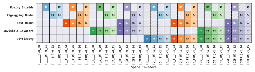
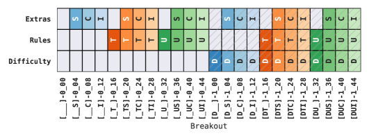
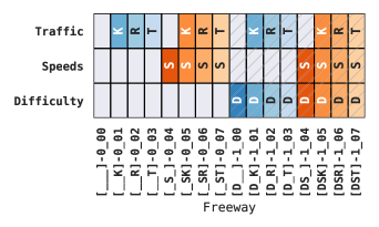
Figure 1: Variant naming convention and factorial design matrices for Space Invaders (top), Breakout (bottom left) and Freeway (bottom right). All factors of variation are categorical and highlighted only when taking different values from default games. Binary factors are abbreviated by their initial, e.g. “Moving Shields” is plotted as ‘M’. Non-binary factors are: Breakout “Rules” with additional values: ‘T’ for “Timed Breakout”, or ‘U’ for “Breakthru”; Breakout “Extras” with additional values: ‘S’ for “Steerable”, ‘C’ for “Catch”, or ‘I’ for “Invisible”; Freeway “Traffic” with levels: ‘K’ for “Thick”, ‘R’ for “Thicker”, or ‘T’ for “Thickest”. Colours indicate the “game mode”, and hatching denotes the “difficulty” switch being activated. Colours and horizontal labels correspond to those used in subsequent figures. Labels include factor abbreviations to supplement the ALE naming conventions.

2.1 ALE Atari as a Transfer Learning Benchmark

With the first version of the Arcade Learning Environment (ALE), Bellemare et al. (2013) gave access to over $50$ different Atari $2600$ game titles through a unified observation and action interface, modelled after the standard reinforcement learning loop. The ALE proved an excellent development test-bed for building general deep RL agents, in no small part due to its diversity and being devoid of experimenter bias, since games were not modified by researchers.

The second and latest version of the ALE (Machado et al., 2018) opens up a wealth of game variations for transfer learning research. This is achieved by emulating functions of “difficulty” and “game select” switches for single-player games. The original cartridges of many game titles came with variations which could be selected and played using these switches. We assign unique identifiers of game variants using the $\mathrm{X}\_\mathrm{YZ}$ notation, with $\mathrm{X}\in\{0,1\}$ denoting the position of the “difficulty” switch, and $\mathrm{YZ}\in\{00,01,02,\dots\}$ indicating the selected “game mode”. Value ranges are game specific and identical to those used by the ALE code-base (Machado et al., 2018). For example, the entry game version of each title is denoted as $0\_00$, which we call the default or basic game. All game variations are different environments that still feature the main concepts of the default. Furthermore, the variants were designed to serve as curricula for human players, hence positive transfer should be possible. Most importantly for our purposes, the ALE remains largely free of experimenter bias. Farebrother et al. (2018) selected a few representative variants from four game titles for experiments. We aim to analyse entire curricula, thus we consider the top three most popular titles from their list, according to sales, and use all their variations, for a total of $72$ distinct environments.

The original designers created game variations using combinations of discrete modifications to a default “entry” game, qualitatively described in accompanying game manuals. We organise these discrete modification into formal factors of variation, following closely the original game design matrices sometimes explicitly plotted in manuals. In Figure 1 we formalise variant naming conventions relative to default games. We briefly explain the meanings of all design factors below, to help build an intuitive understanding of this heterogeneous collection of transfer learning scenarios.

Space Invaders. The player controls an Earth-based laser cannon which can move horizontally along the bottom of the screen. There is a grid of approaching aliens above the player, shooting laser bombs, and the objective of the game is to eliminate all the aliens before they reach the Earth, especially their Command Ships. Three destructible shields above the cannon offer some protection. The game ends once any alien reaches the Earth or the player’s cannon is hit a third time with laser bombs. Game variants are combinations of five binary factors which, when activated, modify the default: (1) The difficulty switch widens the player’s laser cannon, making it an easier target for enemy laser bombs (2) Shields move, and thus are harder to use (3) Enemy laser bombs zigzag, which makes them harder to predict (4) Enemy laser bombs drop faster (5) Invaders are invisible, and only hitting one with the laser briefly illuminates the others . This creates a total of $32$ variants of Space Invader.

Breakout. In order to achieve the best score in any variant, the players need to completely break walls with six layers of coloured bricks by knocking off said bricks with a ball, served and bounced towards the wall with a controllable paddle, which they can move horizontally along the bottom of the screen. The ball will also bounce off of screen edges, except for the bottom edge, where balls either come in contact with the paddle or are lost. Players have a total of five balls at their disposal, and the game ends when all balls are lost. Points are scored when bricks are knocked off the wall, and the ball accelerates on contact with bricks in the top three rows or after twelve consecutive hits. Game variants are created by all combinations of three factors: (1) The binary difficulty switch reduces the paddle’s width by a quarter, making it easier to miss the ball (2) The precise rules which determine how points accumulate: (2-a) with standard “Breakout” rules, e.g. in the default game $(0\_00)$, the player must completely break down two walls of bricks, one after the other, while loosing the fewest balls (2-b) under “Timed Breakout” rules, the player must completely break a single wall as fast as possible, no matter how many of the five balls are used (2-c) with “Breakthru” rules, the player needs to break two walls consecutively, but the ball does not bounce off bricks, unlike in previous variants; the ball keeps going through the wall, quickly picking up speed and accumulating points (3) How the ball is aimed at the wall and “extras”: (3-a) the ball simply bounces off the paddle at a position dependent angle (3-b) the player can also steer the ball in flight (3-c) the player is also able catch the ball and release it at a slower speed (3-d) the wall is invisible and is only briefly illuminated when a brick if knocked off, so the player needs to remember its configuration in order to aim effectively . All factors together define $24$ variants of Breakout.

Freeway. In all variants, the goal of the player is to safely get a chicken across ten lanes of freeway traffic as many times as possible in 2 minutes and $16$ seconds. Variants are constructed as combinations of three design factors: (1) The difficulty switch controls whether the chicken is knocked back one lane, or all the way to the kerb, when hit by incoming vehicles (2) Traffic “thickness”, defined as four levels of traffic density (3) Vehicle speeds across lanes, either constant or randomised . Hence, there are $16$ variants of Freeway.

3 Methodology

Experimental setup. Following the latest ALE benchmark recommendations (Machado et al., 2018), information about player “lives” is not disclosed to agents, and stochasticity is introduced using randomised action replay with probability $25\%$, also known as “sticky actions”. Irrespective of redundancies, agents act using the full set of $18$ actions. Environment observations (Atari screen frames) were pre-processed according to standard practice (Mnih et al., 2015; Hessel et al., 2018). We report agent returns at the end of training, averaged over the last 2 million steps.

Expert Agent Training. We use the Rainbow-IQN model-free deep reinforcement learning algorithm (Hessel et al., 2018; Dabney et al., 2018; Toromanoff et al., 2019) since it is available to the community in several implementations, e.g. Castro et al. (2018), and is effective with widely available commodity hardware and open-source software.

Rainbow (Hessel et al., 2018) collects a number of improvements to DQN (Mnih et al., 2013; 2015), of which we used Double Q-Learning (Van Hasselt et al., 2016), Prioritised Replay (Schaul et al., 2016) and multi-step learning (Sutton & Barto, 2018). Following Castro et al. (2018), we did not use the dueling network architecture (Wang et al., 2016) or noisy networks (Fortunato et al., 2018). We replaced the distributional RL approach C51 (Bellemare et al., 2017) with its more general form (IQN), since it has been shown to be superior (Dabney et al., 2018; Toromanoff et al., 2019).

We used the standard limit on environment interactions of $200$ million steps (Mnih et al., 2015; 2016; Dabney et al., 2018; Machado et al., 2018; Toromanoff et al., 2019). Our study is the first to report Rainbow-IQN results for Atari game variants, hence we use independent hyper-parameter selection for expert training and finetuning experiments.

Expert Agent Finetuning. The experimental setup for finetuning follows closely that for agent training, except for two important differences: (1) We used $10$ million environment steps to adapt to new variants, following Farebrother et al. (2018), which is $20\times$ less data than what variant-experts are trained with. The aim of transfer learning is to reduce resources needed for acquiring new knowledge and behaviours, hence we are interested in improving sample complexity using transfer. (2) The hyper-parameter grid was slightly adapted in order to improve chances of fast learning in this reduced data regime. Further details, including parameter grids, are listed in Appendix B.

Statistical Analyses. A multi-factor Analyses of Variance (ANOVA) (Girden, 1992) is a statistical procedure which investigates the influence that two or more independent variables, or factors, have on a dependent variable. The factors can take two or more categorical values, and experimental designs are often balanced: they use equal numbers of independent observations for all combinations of factor values, no less than three. Other assumptions are normality of deviations from group means, and equal or similar variances, see the discussion in Appendix C. ANOVA can be used to reveal statistically significant evidence against the null-hypothesis that group means are all the same. We study the influence of game design factors, discrete modification to default games, on average returns of learned policies.

Study Limitations. The relationship between hyper-parameters and quality of policies learned with deep RL is complex and poorly understood. Mnih et al. (2015) used task-agnostic DQN hyper-parameters, tuned across a few basic games. Later works introduce several interacting modification, including changes to sets of hyper-parameters (Schaul et al., 2016; Dabney et al., 2018; Toromanoff et al., 2019). With the risk of maximisation bias, we used grid searches per game variant in order to mitigate the greater risks of incorrect inferences about Atari curricula due to poor hyper-parameter settings or divergence. Future works may perform fine-grained sensitivity analyses, using more than two random seeds. Due to computational limitations, we instead report the returns of the top-three agents from our grids.

4 Experiments

We would like to characterise the performance of general transfer learning strategies across heterogeneous scenarios, designed to progressively challenge human players. While the shapes of learning curves are expected to be different between game variants, agent performance is thought to be bounded only by its inductive biases, the learning algorithm and practical limitation on resources, such as computation or interactions (Silver et al., 2021). We say that some game variant is “harder” for a given agent if the average returns of learned policies are lower given equal resource budgets. We aim to explain this in terms of the factors of variation which combinatorially define environments within curricula, knowing that they also impact human player performance. Comparing raw scores across the benchmark is difficult if the underlying tasks are “harder” to learn from scratch, or if variants have different scoring scales, as is sometimes the case here. Hence, we must first establish the performance of our agent learning game variants in isolation. On this basis, we then introduce a relative scoring scheme which enables conclusions to be drawn at the benchmark level.

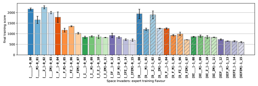
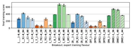
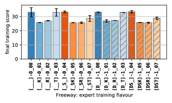
Figure 2: Variant-Expert final raw score distributions, means and standard deviations across the top three experts in their respective hyper-parameter grids, reported for Space Invaders (top), Breakout (bottom left) and Freeway variants (bottom right). In all plots, hatching denotes the “difficulty” switch being activated, and colours indicate the “game mode”. See factorial design matrices for meanings of colour groups (Figure 1).

4.1 Training Variant-Experts

We aim to answer the following questions: (1) Does our agent achieve similar levels of performance when learning variants of the same game from scratch? (2) If not, what explains differences in performance across variants? In Figure 2 we report means and standard deviations of top three variant-experts trained from scratch for 200 million environment steps. Our scores on default games are largely in line with those reported by other implementations of basic IQN agents, e.g. Castro et al. (2018). On remaining variants, we find that Rainbow-IQN performance varies widely for some game titles, less so on Freeway, even with independent hyper-parameter tuning. Overall, our agent’s scores are below variant performance ceilings, suggesting that some game variations may be harder to learn. While this may be at times due to the agent’s inductive biases—in particular, invisible objects—it is unlikely to fully explain observed variation, because such changes to basic games do not always have a detrimental impact on their own. For example, experts achieve significantly different levels of performance on identical variants of Space Invaders, except for visible vs invisible aliens ($0\_00$ vs.$0\_08$). However, experts have virtually equal performance with the same change to environment observations across Breakout variants, visible vs invisible walls of bricks (e.g. $0\_00$ vs. $0\_12$). Rather, we hypothesise that some variants are inherently harder to learn for the chosen agent, and thus a fixed training budget leads to performance differences across variations. This imposes a challenging bottleneck for transfer learning, which places high priority on limiting the resources expended for acquiring behaviours which maximise cumulative returns.

Table 1: Multi-Factor ANOVA (type 3) of Expert Scores vs. design factors.

Space Invaders	$df$	$F$	$PR(>F)$
Difficulty	$1.0$	$115.90$	$5.32e-16$
Invisible Invaders	$1.0$	$1000.59$	$8.67e-41$
Fast Bombs	$1.0$	$314.09$	$2.24e-26$
Zigzagging Bombs	$1.0$	$12.08$	$9.22e-04$
Moving Shields	$1.0$	$125.51$	$9.93e-17$
Interaction	$26.0$	$1341.37$	$5.33e-78$

Breakout	$df$	$F$	$PR(>F)$
Difficulty	$1$	$56.28$	$1.26e-09$
Rules	$2$	$1368.66$	$4.71e-43$
Extras	$3$	$179.84$	$4.22e-26$
Interaction	$17$	$23.04$	$1.91e-17$

Freeway	$df$	$F$	$PR(>F)$
Difficulty	$1$	$1.39$	$2.46e-01$
Speeds	$1$	$91.38$	$6.75e-11$
Traffic	$3$	$453.84$	$2.73e-26$
Interaction	$10$	$274.76$	$4.42e-28$

Statistical Analyses. We verify that variants have meaningful impact on learning by rejecting the null hypothesis that expert performance is the same across all combinations of the design factors which define game variants. We perform multi-factor Analysis of Variance (ANOVA) tests separately for each game title, and report results in Table 1. Interaction effects are statistically significant in all cases, supporting the hypothesis that—although conceptually similar—design factors introduce significant changes to agent learning dynamics, even within the same game. In the post-hoc analyses of differences between groups we found that all factors have a statistically significant effect on agent learning from scratch apart from the “difficulty” factor in Freeway. Further details can be found in Appendix C.

Discussion. Some differences in agent performance across variants were expected due to the qualitative impact of some factors on human play, e.g. changes in the dynamics of state transitions between “Breakout” and “Breakthru” variants, changes in observations such as visible vs. invisible invaders, or the effect of the difficulty switch. It is somewhat surprising that agents learn Freeway variants to similar performance, irrespective of difficulty level. Generally, we find that combinations of factors seem to induce substantially different learning dynamics, each having a significant effect on the final performance of the agent, at least within the standard training budget considered here. Hence, Rainbow-IQN demonstrates different levels of data efficiency across variants, despite their many similarities. A good amount of the variation can be explained by game design factors, which further emphasises the value of this benchmark for systematic and unbiased investigations of transfer with reinforcement learning algorithms.

Considering these empirical findings, as well as the possibility of different asymptotic performance ceilings for different variants, the remainder of the paper reports results relative to variant-expert performance, in order to meaningfully compare transfer learning across variations and curricula on a unified scale. We stress that variant-expert agents are generally not near-optimal. The most surprising results were the comparatively low agent score on “Timed Breakout” variants (orange bars in the bottom left plot of Figure 2), which have identical transition dynamics to regular “Breakout”, but observations differ in that time in seconds is displayed instead of current score. Overall, these findings imply that scores normalised by variant-expert performance can be higher than $100\%$. Nevertheless, a relative scoring scheme accounts for the main effects of factors of variation on our agent’s data efficiency while learning particular game variants. This is essential for meaningful comparisons of transfer learning within and across game curricula.

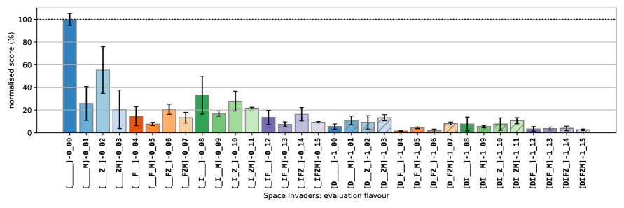
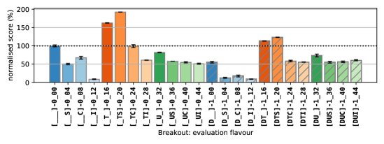
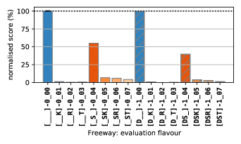
Figure 3: Zero-shot transfer performance of default game experts $(0\_00)$ on all other variants, plotted as normalised scores (percentages) of the final performance of respective variant-experts, reported for Space Invaders (top), Breakout (bottom left) and Freeway variants (bottom right). Hatching denotes the “difficulty” switch being activated, and colours indicate the “game mode”. Colour groups are meaningful with respect to the factorial design matrices of particular game variants (Figure 1).

Table 2: Multi-Factor ANOVA (type 3) of default game expert zero-shot transfer vs. design factors.

Space Invaders	$df$	$F$	$PR(>F)$
Difficulty	$1$	$319.42$	$1.43e-26$
Invisible Invaders	$1$	$208.13$	$8.68e-22$
Fast Bombs	$1$	$250.95$	$7.92e-24$
Zigzagging Bombs	$1$	$6.51$	$1.32e-02$
Moving Shields	$1$	$116.63$	$4.67e-16$
Interaction	$26$	$117.61$	$1.57e-44$

Breakout	$df$	$F$	$PR(>F)$
Difficulty	$1$	$182.22$	$5.83e-18$
Rules	$2$	$476.93$	$2.14e-32$
Extras	$3$	$177.63$	$5.53e-26$
Interaction	$17$	$31.38$	$2.87e-20$

Freeway	$df$	$F$	$PR(>F)$
Difficulty	$1$	$15.87$	$3.66e-04$
Speeds	$1$	$211.61$	$1.17e-15$
Traffic	$3$	$1524.22$	$1.36e-34$
Interaction	$10$	$100.01$	$3.14e-21$

4.2 Zero-shot Transfer using Default Game Experts

Game variants go beyond defaults in ways which are interesting to humans, providing additional challenges by design. Players will often become proficient in the default game, and then attempt to master others; indeed, several game manuals explicitly recommend this approach. Since deep neural networks are known to generalise to similar inputs, and since variants reuse the same visual elements (game sprites), we would like to answer the following questions: (1) How much transfer can be achieved purely through the generalisation power of deep neural networks trained on default games $(0\_00)$? (2) Do factors of variation explain the success of zero-shot transfer (Taylor & Stone, 2009)?

Default game experts are evaluated, without further training, on all remaining variants of their respective games, and normalised scores are reported in Figure 3. Means and standard deviations of zero-shot transfer performance are plotted as percentages of the scores achieved by respective variant-experts, which were trained from scratch using 200 million interaction steps. Rainbow-IQN policies are derived using $\epsilon$-greedy action selection according to value function approximations output by deep neural networks. In the zero-shot transfer case, errors of such predictions are unbounded, but depend on the differences in reward functions and transition dynamics between the source and transfer target MDPs, as well as on the specific function approximation method used. In the case of deep neural networks we have no formal guarantees for the quality of prediction on environment states never encountered in the source task, especially for those which do not exist at all in the source. All things considered, a surprising amount of positive zero-shot transfer is observed in all game domains, due to the sheer generalisation power of deep neural networks. In some cases, e.g. “Timed Breakout” variants, zero-shot transfer results in superior policies to what variant-experts have learned, although data and computational budgets were identical. However, these are exceptions. In the majority of cases, learning on default games results in lower return policies on other variants. That said, the observed zero-shot transfer is not negligible, and it does not appear uniform across game variations, which we investigate next.

Statistical Analyses. In order to answer the second question we check whether zero-shot performance is statistically indistinguishable across game variants, our null hypothesis of interest. We proceed with a multi-factor ANOVA of the dependent variable, here raw zero-shot transfer score, as a function of factors of variation in each game domain. Results reported in Table 2 indicate a statistically significant interactions in all games, meaning that factors play a role in the level of zero-shot transfer observed. In post-hoc analyses we must correct for multiple comparisons, and hence significance at level $\alpha=0.05$ in Space Invaders is achieved for a corrected threshold of $\alpha_{c}=0.0015$ or lower. We find statistically significant effects of all factors except the introduction of “Zigzagging Bombs” in Space Invaders.

Discussion. Zero-shot transfer results provide evidence that the benchmark offers ample challenges for transfer learning approaches. We find the highest levels of zero-shot policy transfer from default Breakout agents to variants, occasionally with higher performance than variant-experts. However, transferred policies are generally far from optimal, which naturally motivates investigations into fast adaptation through transfer learning. Overall, we observe substantial variance in the performance of fixed expert policies trained on defaults, then directly evaluated on all other variations. Although game variants within curricula are related, the statistically significant interaction effects between factors suggest that they are indeed distinct tasks with substantial and diverse “transfer gaps”, necessitating additional learning on top of default game policies. The most significant factors impacting zero-shot transfer were the “difficulty” switch in Space Invaders, the point accumulation “Rules” factor in Breakout, and “Traffic” thickness in Freeway, which we interpret as introducing the broadest differences. It is important to note that such modifications to default games do not easily fit within the more particular sets of assumptions often studied in transfer learning research. It is hard to argue that environment dynamics are precisely the same, or that state spaces are identical in distinct variants. Furthermore, even when observations change in subtle ways, e.g. the “difficulty” switch increases the size of the player’s cannon in Space Invaders, this change has a measurable impact on agent transfer performance, and it is not immediately clear how domain adaptation approaches would mitigate the issue. Hence, we go on to investigate how these diverse “transfer gaps” influence the performance of value-function finetuning, a more general transfer learning algorithm.

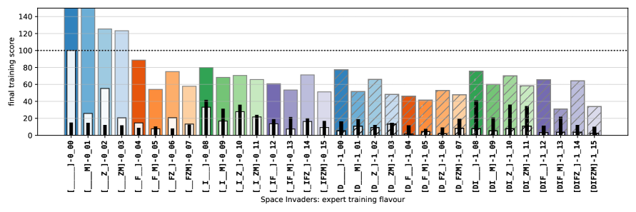
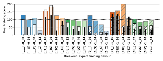
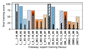
Figure 4: Finetuning performance starting from default game expert $(0\_00)$ on all other variants, plotted as normalised scores (percentages) of the final performance of respective variant-experts, reported for Space Invaders (top), Breakout (bottom left) and Freeway variants (bottom right). Please note that $100\%$ indicates comparable performance with variant-experts, which were trained from scratch with $20\times$ more data than finetuning agents. Black bars show an ablation of finetuning training, starting from scratch rather than from default agent parameters. The delta to is due to transfer learning via agent network parameter initialisation. White bars indicate zero-shot transfer performance of default game agents. The delta to finetuning results represents the net benefit of learning in the transfer target variant. Hatching denotes the “difficulty” switch being on, and colours indicate the “game mode”, see Figure 1 for details.

4.3 Finetuning of Default Game Experts

Zero-shot policy transfer can be substantial, and as such, constitutes an appropriate starting point for fine-tuning on other variants. However, it is not immediately obvious that current RL agents can capitalise on this zero-shot policy transfer to meaningfully speed up learning relative to variant-experts. In order to improve performance on new variants it important that agent representations and predictions are finetuned on data from transfer target tasks. We report results of default game expert finetuning experiments in Figure 4, together with the natural baseline of zero-shot policy transfer from the same experts, and an ablation: learning from scratch for the same amount of environment interaction as used for finetuning. In a majority of cases we find that default expert finetuning outperforms baseline and ablation approaches. Hence, a simple and general algorithm such as Rainbow-IQN finetuning can leverage knowledge acquired in default games to improve performance beyond the zero-shot generalisation offered by its function approximator alone. Note that these gains are significant on the normalised scales induced by variant-expert performance, which account for the different learning dynamics caused by particular game variation, as shown in previous sections.

It is important not to overlook the heterogeneity of these finetuning results within and across curricula. Using a fixed, somewhat generous amount of data to finetune (10 million steps) does allow a substantial amount of performance to be acquired in some cases. Rainbow-IQN agents can also learn to a significant level of performance starting from scratch in this restricted training regime, which we would not have observed without the ablation experiment, e.g. on Freeway variants, but to some extent also on Breakout. Conversely, direct evaluation without training on the transfer target task can confer a competitive level of zero-shot performance, which we necessarily investigated in the previous section. Taken together, we interpret these heterogeneous finetuning results as strong motivation for research on improved general transfer learning algorithms, applicable across many transfer scenarios. But what can help transfer in this very general setting? Intuitively, learning several variants within curricula could offer a solution in the form of transfer using multiple sources, perhaps at the cost of additional complexity.

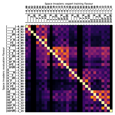
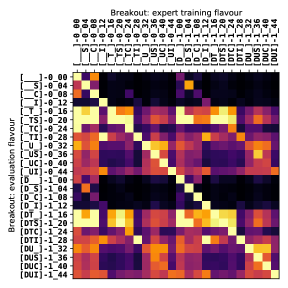
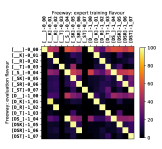
Figure 5: Transfer matrices depicting zero-shot evaluation of Space Invaders (left), Breakout (middle) and Freeway variant-experts (right), plotted as columns, and evaluated on all variants (rows). Values reported as normalised scores (percentages) of respective variant-expert scores.

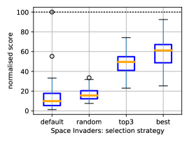
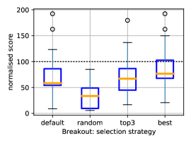
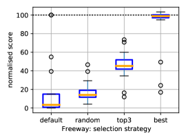
Figure 6: Box-plots of zero-shot normalised score distributions for source task selection strategies on Space Invaders (left), Breakout (middle) and Freeway variants (right): “default” indicates using the default game expert ($0\_00$) policy to act in all variants; the following selection strategies denote ways of choosing policies exclusively from all other variants in their respective domains: “random” means using a randomly chosen expert policy in every evaluation episode; “top3” and “best” strategies require access to some approximation of the transfer matrix to select the top three or best single source policy for each variant, from all other experts.

4.4 Zero-shot Transfer Source Game Selection

In this section, we focus on knowledge in the form of policies learned by experts on other game variants, and we perform an all-to-all zero-shot transfer evaluation, reported as transfer matrices in Figure 5. We observe substantial off-diagonal structure in all games. The default game is not the best single source task in many cases, especially for variants with many factors introducing changes to the basic game. Naturally, we would like to know how well a superior source task selection strategy could perform on average. More precisely, we would like to empirically characterise the average upper bound on zero-shot transfer possible by appropriate selection of a single source policy for any game variant from all the remaining variant-expert policies. We plot the expectation for success of several transfer source task selection strategies in Figure 6, as well as the “best” case selection strategy, which provides an upper bound for what can be achieved by selecting a single variant-expert’s policy. For Freeway we observe strong transfer between policies learned with and without the “difficulty” switch being turned on. Matching the “best” strategy may be costly, e.g. in terms of expert evaluations, so we also report a “top3” selection strategy: zero-shot transfer performance of acting in every episode with one of the “top3” variant-experts at random. This strategy results in over $40\%$ median normalised performance for all curricula. This level of transfer could be achieved at the expense of some target task interactions for ascertaining the quality of all other variant-expert policies on the current game variation. Interestingly, for all game titles, the “top3” strategy is superior to zero-shot transfer from the default games. This cannot be said for the average or “random” choice strategy, which is inferior to zero-shot transfer from default experts in Breakout. These observations motivate further research into automatic selection of variant-expert policies for transfer. The rich off-diagonal structure also recommends the use of Atari game variations as systematic curricula in a continual learning setting, if only for leveraging the potential for policy reuse highlighted by our evaluations.

5 Conclusions

Using Atari curricula, we have demonstrated that general transfer learning approaches, such as zero-shot policy generalisation and single expert model finetuning, lead to significant performance improvements in a large number of diverse transfer learning scenarios that are non-trivial for human players. Our analyses indicate that introducing modifications to basic games in a combinatorial fashion can substantially impact the empirical learning efficiency of a deep RL agent. Furthermore, zero-shot transfer performance from default games alone is also hindered by interactions between modifications. These results highlight the value of learning several variant-experts and reusing their knowledge to quickly find effective policies for new variations. Such strategies have the potential to efficiently match expert performance on transfer target tasks, but require the ability to both accumulate knowledge across game variants, and to appropriately transfer from several source tasks at once. Our study serves as a proof-of-concept that Atari curricula offer an invaluable benchmark of suitable complexity for systematically probing transfer without task engineering.

Appendix A Appendix: Extended Background

Q-learning. Watkins (1989) propose an RL algorithm which iteratively improves a parametric estimate $\hat{Q}_{\theta}~{}=~{}\hat{Q}_{\mathcal{M}}(\cdot,\cdot,\theta)$ of the optimal action-value function $Q_{\mathcal{M}}^{*}$ using the Bellman optimality operator (Bellman, 1957):

$$\hat{Q}_{\theta}(x,a)~{}\leftarrow~{}\mathbb{E}_{\mathcal{T}}\left[\mathcal{R}(x,a,x^{\prime})\right]+\gamma\mathbb{E}_{\mathcal{T}}\left[\max_{a^{\prime}\in\mathcal{A}}\hat{Q}_{\theta}(x^{\prime},a^{\prime})\right].$$

In model-free RL we do not assume explicit knowledge of the transition function $\mathcal{T}$, but the above optimisation can be implemented using samples procured by acting greedily with respect to the estimate $\hat{Q}_{\theta}$ with probability $1-\epsilon$, and choosing actions uniformly at random otherwise. Watkins & Dayan (1992) show that, under certain condition, this procedure converges to $Q^{*}_{\mathcal{M}}$, and an optimal policy can be derived as $\pi^{*}_{\mathcal{M}}(x)=\underset{a\in\mathcal{A}}{\operatorname{arg}\,\operatorname{max}}\;\hat{Q}_{\theta}(x,a)$.

Deep Q-Learning. Mnih et al. (2015) use a convolutional neural network to parameterise $\hat{Q}_{\theta}$, and train the resulting Deep Q-Network (DQN) by iterative minimisation of the squared temporal difference (TD) error:

Samples $(x_{t},a_{t},r_{t},x_{t+1})$ are drawn randomly from a moving-window replay memory, where experience is collected online, and $\theta^{-}$ denotes a slow moving copy of online parameters $\theta$. DQN agents are efficiently trained using RMSProp (Tieleman & Hinton, 2012), a variant of mini-batch stochastic gradient descent (SGD). This approach, with fixed hyper-parameters, was the first to master many classic Atari 2600 games from the Arcade Learning Environment (ALE) (Bellemare et al., 2013) up to a casual human level of performance, using screen pixels as inputs. Several improvements are brought together into the Rainbow agent by Hessel et al. (2018). Dabney et al. (2018) introduce Implicit Quantile Networks (IQN), a principled generalisation of DQN such that the full return distribution $Z_{\mathcal{M}}^{\pi}$ is modelled implicitly through its quantile function, leading to superior performance. Rainbow-IQN was shown to be state-of-the-art at the time for the standard ($200$ million steps) data regime by Toromanoff et al. (2019). This family of algorithms remains the most widely implemented of deep RL approaches.

Deep Reinforcement Learning. Online model-free RL with deep neural networks has been known to suffer from learning instability due to correlations between parameter updates. Stabilisation heuristics proved successful early on, such as off-line, full-batch training (Riedmiller, 2005; Schulman et al., 2015), using a replay memory to decorrelate parameter updates (Mnih et al., 2013; Schaul et al., 2016), and correcting over-estimation errors (Van Hasselt et al., 2016). Mnih et al. (2016) introduced A3C, an online deep RL algorithm which leveraged parallel data generation for stable learning, further improved with auxiliary losses (Jaderberg et al., 2016), and a replay memory (Wang et al., 2016) for better sample efficiency. Deep RL has also been successfully applied to continuous control domains (Lillicrap et al., 2015; Schulman et al., 2015; 2017; Haarnoja et al., 2018). Model-based RL algorithms have proven successful in full information environments which require complex strategy, such as the game of Go (Silver et al., 2016; 2017), several board-games (Schrittwieser et al., 2020) and domains with limited data, such as robotic control (Levine & Koltun, 2013; Levine et al., 2016). Recently, model-based RL approaches with learned models have proven competitive with model-free algorithms on domains with high-dimensional observations, e.g. DreamerV2 (Hafner et al., 2020), and MuZero (Schrittwieser et al., 2020). More complex training strategies have also been successful, such as combining deep RL with supervised learning from human games (Silver et al., 2016), and using self-play, or multi-agent training, leading to human Grandmaster level performance in Starcraft II (Vinyals et al., 2019), and winning against world champions at an e-sports game (Berner et al., 2019). It is important to note that such results are not yet achievable without access to super-computing infrastructure, e.g. thousands of GPUs or TPUs, and complex software stacks for distributed training, with estimated costs in single digit millions of dollars (OpenAI, 2018). Even when such resources are available, agent training can still take many months, so detailed ablations or hyper-parameter tuning become prohibitively expensive (Berner et al., 2019). Hence, improving data and computational efficiency through principled algorithmic innovations is essential for state-of-the-art deep RL.

Appendix B Appendix: Agent Training Details

We tuned relevant hyper-parameters for each game variant in order to avoid sub-optimal performance due to poor settings. Please note that we are the first to report Rainbow-IQN results on Atari variants, and hence we had only the DQN experiments of Farebrother et al. (2018) as a guide, but no results were reported for the standard $200$ million steps training regime, and the two algorithms have many differences which can impact learning dynamics. Farebrother et al. (2018) also used weight decay and dropout to reduce parameter norms and improve the generalisation of trained agents, but final performance was negatively impacted. We share the intuition that models which are closer to a random initialisation have an increased chance to generalise to related tasks, and may even be easier to adapt to new variants during finetuning.

Table 3: Variant-Expert Rainbow-IQN hyper-parameters. When multiple values are specified, the final hyper-parameter was chosen via grid search. Note that each configuration was trained using two different random seeds.

Name	Value(s)	Units/Comments/Attributions
Reward Clipping Bound	$1$	Possible values $\{-1,0,1\}$ (Mnih et al., 2015).
Replay Capacity	$1\,000\,000$	Transitions. (Mnih et al., 2015).
Replay Initial Size	$500\,000$	Transitions. (Hessel et al., 2018).
Initial Policy	$\epsilon=1$	Replay memory initialised using random policy.
Initial Policy $\epsilon$ Annealing Steps	$100\,000$	Linearly annealed to $\epsilon=0.01$ (Mnih et al., 2015).
Behaviour Policy ($\epsilon$-greedy)	$\epsilon=0.01$	The same during training and evaluation.
Action Repeats	$4$	Environment steps. (Mnih et al., 2015).
History Length	$4$	Agent steps. (Mnih et al., 2015).
Discount Factor	$\gamma=0.99$	Mnih et al. (2015).
Multi-step Bootstrap	$n=3$	Hessel et al. (2018).
Double Q-Learning	True	Van Hasselt et al. (2016).
Prioritised Replay	True	Schaul et al. (2016); Hessel et al. (2018).
Prioritisation Exponent	$0.6$	Horgan et al. (2018).
Prioritisation Type	proportional	Hessel et al. (2018).
Prioritisation Importance Sampling	$0.4$	Horgan et al. (2018).
Parallel Environments	$1$	Toromanoff et al. (2019).
Batch size	$\{32,64\}$	Mnih et al. (2015)
Optimiser	Clipped-SGD	Re-scaling gradients with norms larger than $C$.
Gradient Clipping Norm	$C=10$	Largest admissible gradient norm.
Agent Steps per Update	$\{4,8\}$	Agent steps (Mnih et al., 2015).
Learning Rate	$\{${10}^{-6}$,${10}^{-5}$,${10}^{-4}$,${10}^{-3}$\}$	Hessel et al. (2018).
Target Network Update Period	$\{$1000$,$10\,000$\}$	Agent steps (Castro et al., 2018).
Number of $\tau$ Samples	$N=64$	Dabney et al. (2018).
Number of $\tau^{\prime}$ Samples	$N^{\prime}=64$	Dabney et al. (2018).
Number of $\tilde{\tau}$ Samples (Policy)	$K=64$	Dabney et al. (2018).

We replaced RMSProp (Hinton et al., 2006), used by DQN (Mnih et al., 2015), and Adam (Kingma & Ba, 2015), used by Rainbow (Hessel et al., 2018), with Stochastic Gradient Descent (SGD) and gradient norm clipping (Pascanu et al., 2012). Please not that the aforementioned optimisers can provide superior performance, but tend to optimistically increase learning rates when parameter updates are correlated. We used hyper-parameter grid search to choose appropriate learning rates, and we purposefully also including smaller than typical values in the grid; we also allowed larger batch sizes and less frequent parameter updates besides standard values, see Table 3 for details. To further avoid parameter norms increasing due to correlated updates at the start of training, we sampled $500\,000$ transitions in the replay memory before starting learning, using $\epsilon$ decay from fully random behaviour to an $\epsilon$-greedy policy with $\epsilon=0.01$. The intuition behind these choices is that sampling data using a diverse set of behaviours policies will reduce the chances of correlated updates and learning divergence early on in training.

Table 4: Rainbow-IQN expert finetuning hyper-parameters. When multiple values are specified, the final hyper-parameter was chosen via grid search. Note that each configuration was trained using two different random seeds.

Name	Value(s)	Units/Comments/Attributions
Reward Clipping Bound	$1$	Possible values $\{-1,0,1\}$ (Mnih et al., 2015).
Replay Capacity	$1\,000\,000$	Transitions. (Mnih et al., 2015).
Replay Initial Size	$500\,000$	Transitions. (Hessel et al., 2018).
Initial Policy	$\epsilon=1$	Replay memory initialised using random policy.
Initial Policy $\epsilon$ Annealing	$100\,000$	Linearly annealed to $\epsilon=0.01$ (Mnih et al., 2015).
Behaviour Policy ($\epsilon$-greedy)	$\epsilon=0.01$	The same during training and evaluation.
Action Repeats	$4$	Environment steps. (Mnih et al., 2015).
History Length	$4$	Agent steps. (Mnih et al., 2015).
Discount Factor	$\gamma=0.99$	Mnih et al. (2015).
Multi-step Bootstrap	$n=3$	Hessel et al. (2018).
Double Q-Learning	True	Van Hasselt et al. (2016).
Prioritised Replay	True	Schaul et al. (2016); Hessel et al. (2018).
Prioritisation Exponent	$0.6$	Horgan et al. (2018).
Prioritisation Type	proportional	Hessel et al. (2018).
Prioritisation Importance Sampling	$0.4$	Horgan et al. (2018).
Parallel Environments	$1$	Toromanoff et al. (2019).
Batch size	$32$	Mnih et al. (2015)
Optimiser	Clipped-SGD	Re-scaling gradients with norms larger than $C$.
Gradient Clipping Norm	$C\in\{0,10,40\}$	Largest admissible gradient norm. Setting $C=0$ disables gradient clipping.
Agent Steps per Update	$4$	Agent steps (Mnih et al., 2015).
Learning Rate	$\{${10}^{-7}$,${10}^{-6}$,$5\text{\times}{10}^{-6}$$, $${10}^{-5}$,$5\text{\times}{10}^{-5}$,${10}^{-4}$\}$	Hessel et al. (2018).
Target Network Update Period	$10\,000$	Agent steps (Castro et al., 2018).
Number of $\tau$ Samples	$N=64$	Dabney et al. (2018).
Number of $\tau^{\prime}$ Samples	$N^{\prime}=64$	Dabney et al. (2018).
Number of $\tilde{\tau}$ Samples (Policy)	$K=64$	Dabney et al. (2018).

We used a slightly modified hyper-parameter grid for expert finetuning, primarily aimed at finding appropriate learning rates and the optimal levels of gradient clipping, as shown in Table 4. Expert finetuning is performed using a total of $10$ million environment steps, which is $20\times$ less experience and parameter updates compared to expert training from scratch. Hence, we allowed for more lenient gradient clipping, as well as disabling it altogether.

Table 5: Rainbow-IQN Network Architecture.

Name	Value(s)
Convolution Channels	$16,32,32$
Convolution Filter Sizes	$8\times 8,4\times 4,3\times 3$
Convolution Filter Stride	$4\times 4,2\times 2,1\times 1$
Convolution Activations	ReLU, ReLU, Identity
Embedding Hiddens	$1568$
Embedding Activations	ReLU
Latent Dimension	$64$
Combined Hiddens	$256,18$
Combined Activations	ReLU, Identity

Our choice to use hyper-parameter grid searches for both expert training and finetuning has greatly increased the computational costs of this study. We have somewhat offset these costs by reducing the numbers of filters in the convolutional trunk of the agent network, to the same sizes used by Mnih et al. (2013), but we kept the number of convolutional layers at $3$ (Mnih et al., 2015; Dabney et al., 2018). Other network parameters were set according to Dabney et al. (2018), see architecture details in Table 5. These modifications did not significantly impact agent performance, which is largely comparable to results reported by Castro et al. (2018) on default games.

Appendix C Appendix: Statistical Analyses

We used generalised linear models, fit with robust covariance estimates (‘HC3’), to perform multi-factor Analyses of Variance (ANOVA). After rejecting null hypotheses of the omnibus tests, we used Bonferroni corrections for multiple comparisons to perform post-hoc analyses of differences between group means. The desired significance level was $\alpha=0.05$, which we corrected to $\alpha_{c}=0.0015$ for Space Invaders, $\alpha_{c}=0.0020$, for Breakout, $\alpha_{c}=0.0031$ for Freeway, since the numbers of groups are $32$, $24$ and $16$ respectively.

Table 6: Multi-Factor ANOVA (type 3) of Expert Scores vs. design factors, extended tables.

Space Invaders	$sum\_sq$	$df$	$F$	$PR(>F)$
Intercept	$8.18e+07$	$1$	$10862.43$	$3.67e-73$
Difficulty	$8.73e+05$	$1$	$115.90$	$5.32e-16$
Invisible Invaders	$7.54e+06$	$1$	$1000.59$	$8.67e-41$
Fast Bombs	$2.37e+06$	$1$	$314.09$	$2.24e-26$
Zigzagging Bombs	$9.10e+04$	$1$	$12.08$	$9.22e-04$
Moving Shields	$9.46e+05$	$1$	$125.51$	$9.93e-17$
Interaction	$2.63e+08$	$26$	$1341.37$	$5.33e-78$
Residual	$4.82e+05$	$64$
Breakout	$sum\_sq$	$df$	$F$	$PR(>F)$
Intercept	$4.06e+06$	$1$	$7623.13$	$1.49e-54$
Difficulty	$2.99e+04$	$1$	$56.28$	$1.26e-09$
Rules	$1.46e+06$	$2$	$1368.66$	$4.71e-43$
Extras	$2.87e+05$	$3$	$179.84$	$4.22e-26$
Interaction	$2.08e+05$	$17$	$23.04$	$1.91e-17$
Residual	$2.55e+04$	$48$
Freeway	$sum\_sq$	$df$	$F$	$PR(>F)$
Intercept	$27174.26$	$1$	$134697.26$	$1.44e-59$
Difficulty	$0.28$	$1$	$1.39$	$2.46e-01$
Traffic	$274.67$	$3$	$453.84$	$2.73e-26$
Speeds	$18.44$	$1$	$91.38$	$6.75e-11$
Interaction	$554.30$	$10$	$274.76$	$4.42e-28$
Residual	$6.46$	$32$

Table 7: Multi-Factor ANOVA (type 3) of Default game expert zero-shot transfer vs. design factors, extended tables.

Space Invaders	$sum\_sq$	$df$	$F$	$PR(>F)$
Intercept	$3.33e+06$	$1$	$638.21$	$5.35e-35$
Difficulty	$1.66e+06$	$1$	$319.42$	$1.43e-26$
Invisible Invaders	$1.08e+06$	$1$	$208.13$	$8.68e-22$
Fast Bombs	$1.31e+06$	$1$	$250.95$	$7.92e-24$
Zigzagging Bombs	$3.39e+04$	$1$	$6.51$	$1.32e-02$
Moving Shields	$6.08e+05$	$1$	$116.63$	$4.67e-16$
Interaction	$1.59e+07$	$26$	$117.61$	$1.57e-44$
Residual	$3.33e+05$	$64$
Breakout	$sum\_sq$	$df$	$F$	$PR(>F)$
Intercept	$1.36e+06$	$1$	$3436.57$	$2.51e-46$
Difficulty	$7.23e+04$	$1$	$182.22$	$5.83e-18$
Rules	$3.78e+05$	$2$	$476.93$	$2.14e-32$
Extras	$2.11e+05$	$3$	$177.63$	$5.53e-26$
Interaction	$2.12e+05$	$17$	$31.38$	$2.87e-20$
Residual	$1.90e+04$	$48$
Freeway	$sum\_sq$	$df$	$F$	$PR(>F)$
Intercept	$1385.27$	$1$	$2775.16$	$1.14e-32$
Difficulty	$7.92$	$1$	$15.87$	$3.66e-04$
Traffic	$2282.53$	$3$	$1524.22$	$1.36e-34$
Speeds	$105.63$	$1$	$211.61$	$1.17e-15$
Interaction	$499.23$	$10$	$100.01$	$3.14e-21$
Residual	$15.97$	$32$

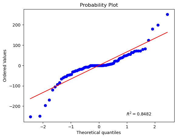
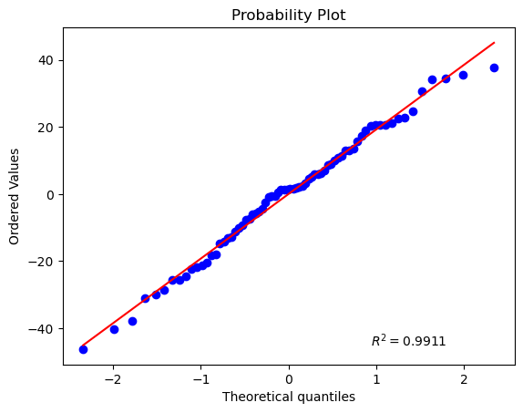
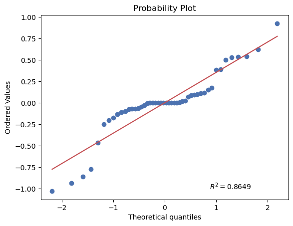
Figure 7: Empirical distribution plots of residuals from Multi-Factor ANOVA of Expert Scores vs. design factors.

C.1 Assumptions:

1. The observations in each group are independent of the observations in every other group. We trained agents independently of each other in all cases, and we selected hyper-parameters for each group (i.e. game variation) independently of others.

2. Normality of measurement errors. For a give game, if we were to re-run the hyper-parameter grid search many times, choose the top 3 agents and average their performance, we assume that such measurements would be normally distributed. We have no reasons to believe that the distribution of the top 3 would be affected by divergence of online learning, one of the likely failure cases. We investigated empirical distribution of residuals from our analyses in Figure 7. We observe some deviation from normality, hence it is best to only draw conclusions based on the strongest significant effects; note that deviations from normality are relevant when effect sizes are very small or when the experimental design is not balanced (Glass & Hopkins, 1996); in our case we use 3 samples per combination of factors (game variation), which is a balanced design.

3. Similar group variances of measurements. We used heteroskedasticity robust variance calculations of type ‘HC3’ (Davidson et al., 1993) to account for observed differences in variance, which we believe are primarily due to sample size.

Appendix D Appendix: Complete Results Tables

In Table 8, Table 9 and Table 10 we provide raw and normalised scores for experts. In Table 11, Table 12, Table 13 we list raw and normalised scores of variant-expert zero-shot transfer.

Table 8: Space Invaders raw and variant-expert normalisation scores in various transfer learning settings and their ablations.

	Raw Scores				Variant-Expert Normalised Scores
Space Invaders (Difficulty & Game Mod)	Variant-Expert $(100\%)$	Finetuning from Scratch	Zero-shot Expert $(0\_00)$	Finetuned Expert $(0\_00)$	Finetuning from Scratch $(\%)$	Zero-shot Expert $(0\_00)$ $(\%)$	Finetuned Expert $(0\_00)$ $(\%)$
$0\_00$	2167.74	326.68	2167.78	33090.00	15.07	100.00	1526.48
$0\_01$	1656.22	244.79	427.31	8949.71	14.78	25.80	540.37
$0\_02$	2250.00	275.85	1243.42	2820.79	12.26	55.26	125.37
$0\_03$	2000.00	235.40	412.60	2465.37	11.77	20.63	123.27
$0\_04$	1783.01	157.97	260.19	1581.55	8.86	14.59	88.70
$0\_05$	1170.38	121.72	89.57	634.09	10.40	7.65	54.18
$0\_06$	1354.09	110.09	280.22	1017.78	8.13	20.69	75.16
$0\_07$	1025.23	128.67	136.02	593.75	12.55	13.27	57.91
$0\_08$	838.10	350.32	278.12	669.79	41.80	33.18	79.92
$0\_09$	875.00	274.31	147.58	597.76	31.35	16.87	68.31
$0\_10$	851.50	307.05	237.02	601.44	36.06	27.84	70.63
$0\_11$	821.58	198.41	178.30	540.59	24.15	21.70	65.80
$0\_12$	921.15	175.94	125.16	559.70	19.10	13.59	60.76
$0\_13$	830.55	179.48	61.88	443.98	21.61	7.45	53.46
$0\_14$	719.11	144.40	117.15	512.50	20.08	16.29	71.27
$0\_15$	697.57	118.31	64.77	357.77	16.96	9.28	51.29
$1\_00$	1938.98	315.28	105.91	1499.32	16.26	5.46	77.33
$1\_01$	1207.91	226.72	131.86	623.19	18.77	10.92	51.59
$1\_02$	1893.35	229.66	174.02	1244.93	12.13	9.19	65.75
$1\_03$	1250.00	183.12	164.62	604.48	14.65	13.17	48.36
$1\_04$	1250.00	145.50	17.18	576.14	11.64	1.37	46.09
$1\_05$	929.55	68.88	40.73	385.40	7.41	4.38	41.46
$1\_06$	993.20	88.99	20.10	524.81	8.96	2.02	52.84
$1\_07$	713.80	135.76	58.13	342.39	19.02	8.14	47.97
$1\_08$	857.34	352.02	65.88	648.87	41.06	7.68	75.68
$1\_09$	886.21	186.99	46.95	530.19	21.10	5.30	59.83
$1\_10$	845.13	304.50	64.59	591.04	36.03	7.64	69.93
$1\_11$	829.79	283.46	87.92	485.00	34.16	10.60	58.45
$1\_12$	729.67	82.16	24.88	476.72	11.26	3.41	65.33
$1\_13$	653.80	141.09	24.23	203.37	21.58	3.71	31.11
$1\_14$	644.76	77.95	24.39	413.87	12.09	3.78	64.19
$1\_15$	600.00	60.90	15.48	204.83	10.15	2.58	34.14

Table 9: Breakout raw and variant-expert normalisation scores in various transfer learning settings and their ablations.

	Raw Scores				Variant-Expert Normalised Scores
Breakout (Difficulty & Game Mode)	Variant-Expert $(100\%)$	Finetuning from Scratch	Zero-shot Expert $(0\_00)$	Finetuned Expert $(0\_00)$	Finetuning from Scratch $(\%)$	Zero-shot Expert $(0\_00)$ $(\%)$	Finetuned Expert $(0\_00)$ $(\%)$
$0\_00$	264.60	6.69	264.60	342.21	2.53	100.00	129.33
$0\_01$	420.10	5.25	212.41	412.43	1.25	50.56	98.17
$0\_02$	298.60	6.51	201.41	325.49	2.18	67.45	109.01
$0\_03$	247.00	6.05	22.02	69.99	2.45	8.92	28.33
$0\_04$	71.90	82.43	116.85	111.95	114.65	162.51	155.70
$0\_05$	55.50	70.97	106.79	101.32	127.87	192.42	182.56
$0\_06$	255.40	72.79	253.50	320.40	28.50	99.26	125.45
$0\_07$	82.40	75.70	50.19	90.10	91.87	60.91	109.35
$0\_08$	386.30	202.85	316.54	385.42	52.51	81.94	99.77
$0\_09$	670.10	251.56	387.64	635.95	37.54	57.85	94.90
$0\_10$	650.20	170.03	357.95	591.00	26.15	55.05	90.90
$0\_11$	385.60	203.56	197.61	356.12	52.79	51.25	92.35
$1\_00$	155.80	14.41	86.12	198.12	9.25	55.28	127.16
$1\_01$	398.00	6.65	50.89	364.01	1.67	12.79	91.46
$1\_02$	335.60	9.46	59.29	223.65	2.82	17.67	66.64
$1\_03$	166.30	14.62	15.19	40.97	8.79	9.14	24.64
$1\_04$	55.50	75.97	62.92	81.70	136.89	113.36	147.20
$1\_05$	51.40	69.62	63.44	80.50	135.44	123.43	156.61
$1\_06$	188.10	92.15	110.40	434.00	48.99	58.69	230.73
$1\_07$	63.20	74.81	35.28	67.71	118.37	55.82	107.13
$1\_08$	353.20	133.44	260.52	362.86	37.78	73.76	102.74
$1\_09$	542.40	217.99	299.91	450.62	40.19	55.29	83.08
$1\_10$	516.90	182.10	293.05	455.30	35.23	56.69	88.08
$1\_11$	361.90	126.34	219.33	343.84	34.91	60.61	95.01

Table 10: Freeway raw and variant-expert normalisation scores in various transfer learning settings and their ablations.

	Raw Scores				Variant-Expert Normalised Scores
Freeway (Difficulty & Game Mode)	Variant-Expert $(100\%)$	Finetuning from Scratch	Zero-shot Expert $(0\_00)$	Finetuned Expert $(0\_00)$	Finetuning from Scratch $(\%)$	Zero-shot Expert $(0\_00)$ $(\%)$	Finetuned Expert $(0\_00)$ $(\%)$
$0\_00$	33.10	23.31	33.14	33.43	70.43	100.12	100.99
$0\_01$	25.83	5.94	0.37	23.55	22.99	1.43	91.18
$0\_02$	27.13	4.98	0.10	11.14	18.35	0.38	41.07
$0\_03$	32.97	11.06	0.24	24.90	33.55	0.73	75.52
$0\_04$	33.30	21.86	18.30	24.55	65.64	54.94	73.73
$0\_05$	25.65	7.96	1.74	9.94	31.03	6.80	38.74
$0\_06$	25.66	7.98	1.53	10.10	31.10	5.98	39.38
$0\_07$	28.74	13.23	1.19	16.49	46.03	4.13	57.38
$1\_00$	33.08	16.94	33.06	33.31	51.20	99.93	100.68
$1\_01$	26.87	5.31	0.23	23.86	19.75	0.86	88.79
$1\_02$	27.34	0.74	0.00	0.00	2.69	0.01	0.00
$1\_03$	32.88	8.16	0.01	23.86	24.83	0.02	72.56
$1\_04$	33.39	17.98	13.16	23.37	53.85	39.41	69.98
$1\_05$	25.85	4.92	1.01	7.94	19.03	3.90	30.71
$1\_06$	25.66	4.67	0.74	7.06	18.21	2.89	27.52
$1\_07$	28.81	7.67	0.42	14.24	26.63	1.48	49.44

Table 11: Space Invaders zero-shot transfer matrix between variant-experts trained from scratch. Top: raw scores, Bottom: Variant-Expert normalised scores (percentages).

$\mathbf{0\_00}$ $\mathbf{0\_01}$ $\mathbf{0\_02}$ $\mathbf{0\_03}$ $\mathbf{0\_04}$ $\mathbf{0\_05}$ $\mathbf{0\_06}$ $\mathbf{0\_07}$ $\mathbf{0\_08}$ $\mathbf{0\_09}$ $\mathbf{0\_10}$ $\mathbf{0\_11}$ $\mathbf{0\_12}$ $\mathbf{0\_13}$ $\mathbf{0\_14}$ $\mathbf{0\_15}$ $\mathbf{1\_00}$ $\mathbf{1\_01}$ $\mathbf{1\_02}$ $\mathbf{1\_03}$ $\mathbf{1\_04}$ $\mathbf{1\_05}$ $\mathbf{1\_06}$ $\mathbf{1\_07}$ $\mathbf{1\_08}$ $\mathbf{1\_09}$ $\mathbf{1\_10}$ $\mathbf{1\_11}$ $\mathbf{1\_12}$ $\mathbf{1\_13}$ $\mathbf{1\_14}$ $\mathbf{1\_15}$ $\mathbf{0\_00}$ $\mathbf{2167.73}$ $1226.64$ n/a n/a $1277.65$ $635.01$ $1142.10$ $814.03$ $652.46$ n/a $493.27$ $559.81$ $611.71$ $433.68$ $487.11$ $435.32$ $319.10$ $261.45$ $431.43$ n/a n/a $255.91$ $415.88$ $433.60$ $347.61$ $288.38$ $342.86$ $318.14$ $351.97$ $320.25$ $381.26$ n/a $\mathbf{0\_01}$ $427.30$ $\mathbf{1656.22}$ n/a n/a $398.31$ $695.62$ $307.10$ $810.83$ $256.30$ n/a $226.23$ $538.11$ $257.92$ $488.21$ $242.52$ $446.40$ $179.16$ $252.14$ $209.43$ n/a n/a $266.06$ $178.37$ $430.60$ $221.26$ $220.32$ $213.98$ $258.34$ $239.40$ $228.53$ $205.37$ n/a $\mathbf{0\_02}$ $1243.41$ $803.94$ $\mathbf{2250.00}$ n/a $1049.00$ $592.73$ $1172.30$ $768.08$ $544.38$ n/a $631.30$ $478.63$ $510.51$ $313.97$ $537.14$ $418.64$ $203.39$ $196.40$ $485.90$ n/a n/a $263.55$ $407.57$ $462.79$ $344.60$ $287.10$ $353.60$ $193.09$ $341.93$ $192.75$ $337.08$ n/a $\mathbf{0\_03}$ $412.60$ $956.95$ n/a $\mathbf{2000.00}$ $421.62$ $638.11$ $381.99$ $962.81$ $261.09$ n/a $285.93$ $626.83$ $221.58$ $444.65$ $220.87$ $445.52$ $134.44$ $160.69$ $280.40$ n/a n/a $279.23$ $191.18$ $461.67$ $200.20$ $238.46$ $230.91$ $210.58$ $262.13$ $263.51$ $193.16$ n/a $\mathbf{0\_04}$ $260.18$ $215.73$ n/a n/a $\mathbf{1783.01}$ $641.93$ $1155.01$ $816.48$ $153.75$ n/a $113.41$ $193.99$ $378.42$ $370.50$ $349.20$ $275.14$ $159.72$ $112.10$ $199.07$ n/a n/a $160.48$ $280.42$ $264.98$ $135.34$ $121.49$ $114.22$ $114.33$ $299.31$ $201.93$ $258.39$ n/a $\mathbf{0\_05}$ $89.57$ $285.14$ n/a n/a $216.40$ $\mathbf{1170.38}$ $162.68$ $1081.71$ $83.82$ n/a $59.62$ $263.71$ $186.22$ $347.12$ $74.30$ $317.68$ $76.42$ $75.42$ $66.74$ n/a n/a $129.81$ $76.79$ $223.49$ $56.11$ $92.51$ $67.66$ $92.65$ $112.65$ $149.86$ $77.24$ n/a $\mathbf{0\_06}$ $280.21$ $233.71$ n/a n/a $857.53$ $393.64$ $\mathbf{1354.09}$ $703.49$ $106.65$ n/a $196.21$ $166.18$ $321.49$ $245.97$ $444.50$ $280.50$ $65.88$ $63.20$ $201.13$ n/a n/a $94.08$ $217.32$ $272.66$ $117.43$ $105.91$ $98.83$ $89.33$ $218.75$ $91.54$ $158.64$ n/a $\mathbf{0\_07}$ $136.01$ $248.04$ n/a n/a $203.98$ $471.63$ $167.28$ $\mathbf{1025.23}$ $92.07$ n/a $90.64$ $198.15$ $131.36$ $369.47$ $118.60$ $345.42$ $69.81$ $71.70$ $79.28$ n/a n/a $130.60$ $84.59$ $264.34$ $70.71$ $76.03$ $60.29$ $85.34$ $114.32$ $113.63$ $95.75$ n/a $\mathbf{0\_08}$ $278.12$ $188.25$ n/a n/a $289.53$ $269.12$ $332.04$ $343.24$ $\mathbf{838.10}$ n/a $562.71$ $499.90$ $546.12$ $465.03$ $409.32$ $457.66$ $284.95$ $256.66$ $348.43$ n/a n/a $141.53$ $322.53$ $279.77$ $321.20$ $283.45$ $335.56$ $285.66$ $439.94$ $377.17$ $389.71$ n/a $\mathbf{0\_09}$ $147.57$ $211.99$ n/a n/a $210.19$ $281.98$ $207.78$ $345.67$ $260.52$ $\mathbf{875.00}$ $250.95$ $743.68$ $315.27$ $618.51$ $249.91$ $584.36$ $193.05$ $278.38$ $234.58$ n/a n/a $152.39$ $143.94$ $321.93$ $273.79$ $339.74$ $226.15$ $253.88$ $281.30$ $403.79$ $257.53$ n/a $\mathbf{0\_10}$ $237.01$ $136.52$ n/a n/a $208.30$ $211.16$ $301.21$ $297.45$ $609.73$ n/a $\mathbf{851.50}$ $524.04$ $493.16$ $399.02$ $582.78$ $472.46$ $271.50$ $269.45$ $359.70$ n/a n/a $118.24$ $341.49$ $277.43$ $325.37$ $263.68$ $305.34$ $237.70$ $437.22$ $333.73$ $381.50$ n/a $\mathbf{0\_11}$ $178.31$ $132.07$ n/a n/a $156.55$ $221.98$ $216.14$ $288.84$ $236.65$ n/a $225.74$ $\mathbf{821.58}$ $213.75$ $462.73$ $249.24$ $522.65$ $170.25$ $229.92$ $213.85$ n/a n/a $134.46$ $115.08$ $299.32$ $180.09$ $242.96$ $164.35$ $216.42$ $254.82$ $355.71$ $221.84$ n/a $\mathbf{0\_12}$ $125.17$ $109.48$ n/a n/a $265.58$ $256.49$ $270.00$ $367.36$ $262.95$ n/a $258.83$ $185.46$ $\mathbf{921.15}$ $545.45$ $527.67$ $430.36$ $138.29$ $129.09$ $156.80$ n/a n/a $87.58$ $190.86$ $231.15$ $155.40$ $134.94$ $129.77$ $107.84$ $359.36$ $267.96$ $269.76$ n/a $\mathbf{0\_13}$ $61.88$ $96.87$ n/a n/a $84.99$ $228.46$ $91.87$ $344.11$ $94.48$ n/a $72.88$ $167.42$ $170.52$ $\mathbf{830.55}$ $121.79$ $420.37$ $73.03$ $72.16$ $65.63$ n/a n/a $74.59$ $66.10$ $141.61$ $105.35$ $76.18$ $58.00$ $61.93$ $100.54$ $242.57$ $79.40$ n/a $\mathbf{0\_14}$ $117.15$ $68.85$ n/a n/a $151.31$ $152.76$ $235.26$ $242.60$ $323.11$ n/a $309.49$ $205.31$ $474.94$ $310.06$ $\mathbf{719.11}$ $419.77$ $120.96$ $113.80$ $149.01$ n/a n/a $73.12$ $207.50$ $201.94$ $123.73$ $123.43$ $132.91$ $128.75$ $318.70$ $224.31$ $253.48$ n/a $\mathbf{0\_15}$ $64.77$ $60.20$ n/a n/a $77.58$ $127.77$ $104.03$ $215.53$ $40.08$ n/a $77.03$ $175.63$ $65.65$ $330.24$ $132.37$ $\mathbf{697.57}$ $51.41$ $53.32$ $69.31$ n/a n/a $31.63$ $56.52$ $120.45$ $59.99$ $75.81$ $45.78$ $71.02$ $98.78$ $151.63$ $73.34$ n/a $\mathbf{1\_00}$ $105.91$ $191.68$ n/a n/a $231.92$ $191.04$ $348.10$ $251.05$ $234.89$ n/a $220.85$ $186.18$ $188.42$ $133.97$ $162.52$ $184.92$ $\mathbf{1938.98}$ $641.59$ $1122.48$ n/a n/a $455.29$ $780.91$ $423.87$ $582.11$ $511.37$ $463.28$ $419.86$ $413.38$ $301.78$ $457.32$ n/a $\mathbf{1\_01}$ $131.85$ $265.95$ n/a n/a $134.62$ $231.63$ $159.69$ $415.00$ $160.05$ n/a $100.67$ $184.05$ $74.81$ $259.57$ $98.16$ $188.38$ $404.39$ $\mathbf{1207.91}$ $333.56$ n/a n/a $528.02$ $225.36$ $569.63$ $199.68$ $573.80$ $188.97$ $358.21$ $190.26$ $368.63$ $191.31$ n/a $\mathbf{1\_02}$ $174.03$ $222.04$ n/a n/a $213.52$ $175.89$ $351.12$ $260.29$ $239.46$ n/a $225.72$ $183.21$ $179.41$ $137.67$ $242.65$ $191.29$ $1198.66$ $601.37$ $\mathbf{1893.35}$ n/a n/a $416.56$ $896.36$ $457.22$ $521.08$ $356.06$ $502.72$ $385.58$ $430.59$ $246.24$ $466.75$ n/a $\mathbf{1\_03}$ $164.62$ $295.00$ n/a n/a $180.85$ $246.92$ $184.79$ $391.08$ $151.69$ n/a $141.87$ $233.03$ $116.81$ $275.91$ $135.91$ $232.86$ $317.77$ $721.90$ $388.63$ $\mathbf{1250.00}$ n/a $613.93$ $278.01$ $687.77$ $213.58$ $468.22$ $228.57$ $434.95$ $206.96$ $353.65$ $198.17$ n/a $\mathbf{1\_04}$ $17.18$ $39.94$ n/a n/a $72.17$ $73.74$ $171.25$ $146.08$ $31.43$ n/a $26.42$ $46.56$ $38.92$ $58.15$ $56.58$ $93.45$ $256.30$ $85.59$ $226.17$ n/a $\mathbf{1250.00}$ $493.51$ $911.02$ $247.24$ $251.53$ $93.45$ $43.39$ $89.31$ $522.87$ $247.59$ $399.91$ n/a $\mathbf{1\_05}$ $40.73$ $78.06$ n/a n/a $32.99$ $111.50$ $43.28$ $152.50$ $49.97$ n/a $19.09$ $46.20$ $49.72$ $123.52$ $32.72$ $44.94$ $56.91$ $63.36$ $71.40$ n/a n/a $\mathbf{929.55}$ $53.66$ $421.89$ $23.55$ $159.70$ $44.02$ $80.09$ $98.63$ $208.80$ $73.11$ n/a $\mathbf{1\_06}$ $20.11$ $64.43$ n/a n/a $79.41$ $57.43$ $181.01$ $150.63$ $29.25$ n/a $37.58$ $47.99$ $77.44$ $62.48$ $85.28$ $103.79$ $142.69$ $77.59$ $218.72$ n/a n/a $349.72$ $\mathbf{993.20}$ $332.18$ $133.77$ $71.14$ $116.36$ $70.96$ $350.63$ $155.18$ $373.39$ n/a $\mathbf{1\_07}$ $58.13$ $80.39$ n/a n/a $62.19$ $106.69$ $43.02$ $176.06$ $59.46$ n/a $26.88$ $49.48$ $51.82$ $111.04$ $55.13$ $79.42$ $65.18$ $166.86$ $87.72$ n/a n/a $369.11$ $96.38$ $\mathbf{713.80}$ $61.86$ $66.56$ $50.73$ $79.51$ $58.93$ $210.63$ $66.20$ n/a $\mathbf{1\_08}$ $65.88$ $39.27$ n/a n/a $75.03$ $54.60$ $125.95$ $171.93$ $227.22$ n/a $164.64$ $160.11$ $164.30$ $138.99$ $227.44$ $228.79$ $325.62$ $112.96$ $243.82$ n/a n/a $132.85$ $252.64$ $255.02$ $\mathbf{857.34}$ $575.49$ $487.97$ $430.12$ $563.76$ $388.33$ $532.14$ n/a $\mathbf{1\_09}$ $46.95$ $20.08$ n/a n/a $79.64$ $55.61$ $112.82$ $136.79$ $138.78$ n/a $114.94$ $289.07$ $109.66$ $255.08$ $125.89$ $314.53$ $192.00$ $168.46$ $141.16$ n/a n/a $172.80$ $110.51$ $232.78$ $185.38$ $\mathbf{886.21}$ $196.16$ $652.13$ $194.37$ $539.33$ $241.20$ n/a $\mathbf{1\_10}$ $64.59$ $44.83$ n/a n/a $82.79$ $59.59$ $141.13$ $175.58$ $196.17$ n/a $278.41$ $180.00$ $195.27$ $181.88$ $179.84$ $231.38$ $288.33$ $96.09$ $262.27$ n/a n/a $131.14$ $238.28$ $273.28$ $667.74$ $466.08$ $\mathbf{845.13}$ $431.91$ $573.51$ $391.16$ $622.36$ n/a $\mathbf{1\_11}$ $87.92$ $33.37$ n/a n/a $81.48$ $45.28$ $106.02$ $112.97$ $111.72$ n/a $127.64$ $248.20$ $107.85$ $246.03$ $143.87$ $271.70$ $165.37$ $110.57$ $157.93$ n/a n/a $148.60$ $155.56$ $209.26$ $140.54$ $551.10$ $192.69$ $\mathbf{829.79}$ $149.51$ $462.69$ $254.89$ n/a $\mathbf{1\_12}$ $24.88$ $19.64$ n/a n/a $43.62$ $25.95$ $76.46$ $119.24$ $33.52$ n/a $24.29$ $45.24$ $79.15$ $89.97$ $58.67$ $112.51$ $95.20$ $28.11$ $66.99$ n/a n/a $138.56$ $181.19$ $138.08$ $183.91$ $92.49$ $115.60$ $80.00$ $\mathbf{729.67}$ $316.37$ $461.11$ n/a $\mathbf{1\_13}$ $24.23$ $17.34$ n/a n/a $26.56$ $32.70$ $31.96$ $81.56$ $28.29$ n/a $35.87$ $68.44$ $29.35$ $97.21$ $37.14$ $157.20$ $38.65$ $38.25$ $36.94$ n/a n/a $129.03$ $50.84$ $99.96$ $33.84$ $165.60$ $46.52$ $91.87$ $60.05$ $\mathbf{653.80}$ $82.48$ n/a $\mathbf{1\_14}$ $24.39$ $19.57$ n/a n/a $39.68$ $30.17$ $69.22$ $91.19$ $33.32$ n/a $32.22$ $51.49$ $64.71$ $71.02$ $71.50$ $139.19$ $93.73$ $28.15$ $86.07$ n/a n/a $91.43$ $203.00$ $159.92$ $279.36$ $108.50$ $189.74$ $114.37$ $479.67$ $228.41$ $\mathbf{644.76}$ n/a $\mathbf{1\_15}$ $15.48$ $13.61$ n/a n/a $33.61$ $11.15$ $30.21$ $37.76$ $37.73$ n/a $29.49$ $88.47$ $35.93$ $80.87$ $65.00$ $146.28$ $43.07$ $27.54$ $31.50$ n/a n/a $109.60$ $42.69$ $142.00$ $39.79$ $116.29$ $47.45$ $181.65$ $54.56$ $256.98$ $64.38$ $\mathbf{600.00}$ $\mathbf{0\_00}$ $\mathbf{0\_01}$ $\mathbf{0\_02}$ $\mathbf{0\_03}$ $\mathbf{0\_04}$ $\mathbf{0\_05}$ $\mathbf{0\_06}$ $\mathbf{0\_07}$ $\mathbf{0\_08}$ $\mathbf{0\_09}$ $\mathbf{0\_10}$ $\mathbf{0\_11}$ $\mathbf{0\_12}$ $\mathbf{0\_13}$ $\mathbf{0\_14}$ $\mathbf{0\_15}$ $\mathbf{1\_00}$ $\mathbf{1\_01}$ $\mathbf{1\_02}$ $\mathbf{1\_03}$ $\mathbf{1\_04}$ $\mathbf{1\_05}$ $\mathbf{1\_06}$ $\mathbf{1\_07}$ $\mathbf{1\_08}$ $\mathbf{1\_09}$ $\mathbf{1\_10}$ $\mathbf{1\_11}$ $\mathbf{1\_12}$ $\mathbf{1\_13}$ $\mathbf{1\_14}$ $\mathbf{1\_15}$ $\mathbf{0\_00}$ $\mathbf{100.00}$ $56.59$ n/a n/a $58.94$ $29.29$ $52.69$ $37.55$ $30.10$ n/a $22.76$ $25.82$ $28.22$ $20.01$ $22.47$ $20.08$ $14.72$ $12.06$ $19.90$ n/a n/a $11.81$ $19.19$ $20.00$ $16.04$ $13.30$ $15.82$ $14.68$ $16.24$ $14.77$ $17.59$ n/a $\mathbf{0\_01}$ $25.80$ $\mathbf{100.00}$ n/a n/a $24.05$ $42.00$ $18.54$ $48.96$ $15.48$ n/a $13.66$ $32.49$ $15.57$ $29.48$ $14.64$ $26.95$ $10.82$ $15.22$ $12.64$ n/a n/a $16.06$ $10.77$ $26.00$ $13.36$ $13.30$ $12.92$ $15.60$ $14.45$ $13.80$ $12.40$ n/a $\mathbf{0\_02}$ $55.26$ $35.73$ $\mathbf{100.00}$ n/a $46.62$ $26.34$ $52.10$ $34.14$ $24.19$ n/a $28.06$ $21.27$ $22.69$ $13.95$ $23.87$ $18.61$ $9.04$ $8.73$ $21.60$ n/a n/a $11.71$ $18.11$ $20.57$ $15.32$ $12.76$ $15.72$ $8.58$ $15.20$ $8.57$ $14.98$ n/a $\mathbf{0\_03}$ $20.63$ $47.85$ n/a $\mathbf{100.00}$ $21.08$ $31.91$ $19.10$ $48.14$ $13.05$ n/a $14.30$ $31.34$ $11.08$ $22.23$ $11.04$ $22.28$ $6.72$ $8.03$ $14.02$ n/a n/a $13.96$ $9.56$ $23.08$ $10.01$ $11.92$ $11.55$ $10.53$ $13.11$ $13.18$ $9.66$ n/a $\mathbf{0\_04}$ $14.59$ $12.10$ n/a n/a $\mathbf{100.00}$ $36.00$ $64.78$ $45.79$ $8.62$ n/a $6.36$ $10.88$ $21.22$ $20.78$ $19.58$ $15.43$ $8.96$ $6.29$ $11.16$ n/a n/a $9.00$ $15.73$ $14.86$ $7.59$ $6.81$ $6.41$ $6.41$ $16.79$ $11.33$ $14.49$ n/a $\mathbf{0\_05}$ $7.65$ $24.36$ n/a n/a $18.49$ $\mathbf{100.00}$ $13.90$ $92.42$ $7.16$ n/a $5.09$ $22.53$ $15.91$ $29.66$ $6.35$ $27.14$ $6.53$ $6.44$ $5.70$ n/a n/a $11.09$ $6.56$ $19.09$ $4.79$ $7.90$ $5.78$ $7.92$ $9.62$ $12.80$ $6.60$ n/a $\mathbf{0\_06}$ $20.69$ $17.26$ n/a n/a $63.33$ $29.07$ $\mathbf{100.00}$ $51.95$ $7.88$ n/a $14.49$ $12.27$ $23.74$ $18.17$ $32.83$ $20.72$ $4.87$ $4.67$ $14.85$ n/a n/a $6.95$ $16.05$ $20.14$ $8.67$ $7.82$ $7.30$ $6.60$ $16.15$ $6.76$ $11.72$ n/a $\mathbf{0\_07}$ $13.27$ $24.19$ n/a n/a $19.90$ $46.00$ $16.32$ $\mathbf{100.00}$ $8.98$ n/a $8.84$ $19.33$ $12.81$ $36.04$ $11.57$ $33.69$ $6.81$ $6.99$ $7.73$ n/a n/a $12.74$ $8.25$ $25.78$ $6.90$ $7.42$ $5.88$ $8.32$ $11.15$ $11.08$ $9.34$ n/a $\mathbf{0\_08}$ $33.18$ $22.46$ n/a n/a $34.55$ $32.11$ $39.62$ $40.95$ $\mathbf{100.00}$ n/a $67.14$ $59.65$ $65.16$ $55.49$ $48.84$ $54.61$ $34.00$ $30.62$ $41.57$ n/a n/a $16.89$ $38.48$ $33.38$ $38.32$ $33.82$ $40.04$ $34.08$ $52.49$ $45.00$ $46.50$ n/a $\mathbf{0\_09}$ $16.87$ $24.23$ n/a n/a $24.02$ $32.23$ $23.75$ $39.51$ $29.77$ $\mathbf{100.00}$ $28.68$ $84.99$ $36.03$ $70.69$ $28.56$ $66.78$ $22.06$ $31.81$ $26.81$ n/a n/a $17.42$ $16.45$ $36.79$ $31.29$ $38.83$ $25.85$ $29.01$ $32.15$ $46.15$ $29.43$ n/a $\mathbf{0\_10}$ $27.83$ $16.03$ n/a n/a $24.46$ $24.80$ $35.37$ $34.93$ $71.61$ n/a $\mathbf{100.00}$ $61.54$ $57.92$ $46.86$ $68.44$ $55.49$ $31.88$ $31.64$ $42.24$ n/a n/a $13.89$ $40.10$ $32.58$ $38.21$ $30.97$ $35.86$ $27.92$ $51.35$ $39.19$ $44.80$ n/a $\mathbf{0\_11}$ $21.70$ $16.07$ n/a n/a $19.05$ $27.02$ $26.31$ $35.16$ $28.80$ n/a $27.48$ $\mathbf{100.00}$ $26.02$ $56.32$ $30.34$ $63.61$ $20.72$ $27.98$ $26.03$ n/a n/a $16.37$ $14.01$ $36.43$ $21.92$ $29.57$ $20.00$ $26.34$ $31.02$ $43.29$ $27.00$ n/a $\mathbf{0\_12}$ $13.59$ $11.88$ n/a n/a $28.83$ $27.84$ $29.31$ $39.88$ $28.54$ n/a $28.10$ $20.13$ $\mathbf{99.99}$ $59.21$ $57.28$ $46.72$ $15.01$ $14.01$ $17.02$ n/a n/a $9.51$ $20.72$ $25.09$ $16.87$ $14.65$ $14.09$ $11.71$ $39.01$ $29.09$ $29.28$ n/a $\mathbf{0\_13}$ $7.45$ $11.66$ n/a n/a $10.23$ $27.51$ $11.06$ $41.43$ $11.37$ n/a $8.77$ $20.16$ $20.53$ $\mathbf{99.99}$ $14.66$ $50.61$ $8.79$ $8.69$ $7.90$ n/a n/a $8.98$ $7.96$ $17.05$ $12.68$ $9.17$ $6.98$ $7.46$ $12.10$ $29.20$ $9.56$ n/a $\mathbf{0\_14}$ $16.29$ $9.57$ n/a n/a $21.04$ $21.24$ $32.72$ $33.74$ $44.93$ n/a $43.04$ $28.55$ $66.05$ $43.12$ $\mathbf{100.00}$ $58.37$ $16.82$ $15.83$ $20.72$ n/a n/a $10.17$ $28.86$ $28.08$ $17.21$ $17.16$ $18.48$ $17.90$ $44.32$ $31.19$ $35.25$ n/a $\mathbf{0\_15}$ $9.29$ $8.63$ n/a n/a $11.12$ $18.32$ $14.91$ $30.90$ $5.75$ n/a $11.04$ $25.18$ $9.41$ $47.34$ $18.98$ $\mathbf{100.00}$ $7.37$ $7.64$ $9.94$ n/a n/a $4.53$ $8.10$ $17.27$ $8.60$ $10.87$ $6.56$ $10.18$ $14.16$ $21.74$ $10.51$ n/a $\mathbf{1\_00}$ $5.46$ $9.89$ n/a n/a $11.96$ $9.85$ $17.95$ $12.95$ $12.11$ n/a $11.39$ $9.60$ $9.72$ $6.91$ $8.38$ $9.54$ $\mathbf{100.00}$ $33.09$ $57.89$ n/a n/a $23.48$ $40.27$ $21.86$ $30.02$ $26.37$ $23.89$ $21.65$ $21.32$ $15.56$ $23.59$ n/a $\mathbf{1\_01}$ $10.92$ $22.02$ n/a n/a $11.15$ $19.18$ $13.22$ $34.36$ $13.25$ n/a $8.33$ $15.24$ $6.19$ $21.49$ $8.13$ $15.60$ $33.48$ $\mathbf{100.00}$ $27.61$ n/a n/a $43.71$ $18.66$ $47.16$ $16.53$ $47.50$ $15.64$ $29.66$ $15.75$ $30.52$ $15.84$ n/a $\mathbf{1\_02}$ $9.19$ $11.73$ n/a n/a $11.28$ $9.29$ $18.54$ $13.75$ $12.65$ n/a $11.92$ $9.68$ $9.48$ $7.27$ $12.82$ $10.10$ $63.31$ $31.76$ $\mathbf{100.00}$ n/a n/a $22.00$ $47.34$ $24.15$ $27.52$ $18.81$ $26.55$ $20.36$ $22.74$ $13.01$ $24.65$ n/a $\mathbf{1\_03}$ $13.17$ $23.60$ n/a n/a $14.47$ $19.75$ $14.78$ $31.29$ $12.14$ n/a $11.35$ $18.64$ $9.34$ $22.07$ $10.87$ $18.63$ $25.42$ $57.75$ $31.09$ $\mathbf{100.00}$ n/a $49.11$ $22.24$ $55.02$ $17.09$ $37.46$ $18.29$ $34.80$ $16.56$ $28.29$ $15.85$ n/a $\mathbf{1\_04}$ $1.37$ $3.19$ n/a n/a $5.77$ $5.90$ $13.70$ $11.69$ $2.51$ n/a $2.11$ $3.72$ $3.11$ $4.65$ $4.53$ $7.48$ $20.50$ $6.85$ $18.09$ n/a $\mathbf{100.00}$ $39.48$ $72.88$ $19.78$ $20.12$ $7.48$ $3.47$ $7.14$ $41.83$ $19.81$ $31.99$ n/a $\mathbf{1\_05}$ $4.38$ $8.40$ n/a n/a $3.55$ $12.00$ $4.66$ $16.41$ $5.38$ n/a $2.05$ $4.97$ $5.35$ $13.29$ $3.52$ $4.84$ $6.12$ $6.82$ $7.68$ n/a n/a $\mathbf{100.01}$ $5.77$ $45.39$ $2.53$ $17.18$ $4.74$ $8.62$ $10.61$ $22.46$ $7.86$ n/a $\mathbf{1\_06}$ $2.02$ $6.49$ n/a n/a $8.00$ $5.78$ $18.23$ $15.17$ $2.94$ n/a $3.78$ $4.83$ $7.80$ $6.29$ $8.59$ $10.45$ $14.37$ $7.81$ $22.02$ n/a n/a $35.21$ $\mathbf{100.00}$ $33.45$ $13.47$ $7.16$ $11.72$ $7.14$ $35.30$ $15.62$ $37.59$ n/a $\mathbf{1\_07}$ $8.14$ $11.26$ n/a n/a $8.71$ $14.95$ $6.03$ $24.67$ $8.33$ n/a $3.77$ $6.93$ $7.26$ $15.56$ $7.72$ $11.13$ $9.13$ $23.38$ $12.29$ n/a n/a $51.71$ $13.50$ $\mathbf{100.00}$ $8.67$ $9.32$ $7.11$ $11.14$ $8.26$ $29.51$ $9.27$ n/a $\mathbf{1\_08}$ $7.68$ $4.58$ n/a n/a $8.75$ $6.37$ $14.69$ $20.05$ $26.50$ n/a $19.20$ $18.68$ $19.16$ $16.21$ $26.53$ $26.69$ $37.98$ $13.18$ $28.44$ n/a n/a $15.50$ $29.47$ $29.75$ $\mathbf{100.00}$ $67.13$ $56.92$ $50.17$ $65.76$ $45.30$ $62.07$ n/a $\mathbf{1\_09}$ $5.30$ $2.27$ n/a n/a $8.99$ $6.27$ $12.73$ $15.44$ $15.66$ n/a $12.97$ $32.62$ $12.37$ $28.78$ $14.21$ $35.49$ $21.67$ $19.01$ $15.93$ n/a n/a $19.50$ $12.47$ $26.27$ $20.92$ $\mathbf{100.00}$ $22.13$ $73.59$ $21.93$ $60.86$ $27.22$ n/a $\mathbf{1\_10}$ $7.64$ $5.30$ n/a n/a $9.80$ $7.05$ $16.70$ $20.78$ $23.21$ n/a $32.94$ $21.30$ $23.11$ $21.52$ $21.28$ $27.38$ $34.12$ $11.37$ $31.03$ n/a n/a $15.52$ $28.20$ $32.34$ $79.01$ $55.15$ $\mathbf{100.00}$ $51.11$ $67.86$ $46.29$ $73.64$ n/a $\mathbf{1\_11}$ $10.60$ $4.02$ n/a n/a $9.82$ $5.46$ $12.78$ $13.61$ $13.46$ n/a $15.38$ $29.91$ $13.00$ $29.65$ $17.34$ $32.74$ $19.93$ $13.33$ $19.03$ n/a n/a $17.91$ $18.75$ $25.22$ $16.94$ $66.41$ $23.22$ $\mathbf{100.00}$ $18.02$ $55.76$ $30.72$ n/a $\mathbf{1\_12}$ $3.41$ $2.69$ n/a n/a $5.98$ $3.56$ $10.48$ $16.34$ $4.59$ n/a $3.33$ $6.20$ $10.85$ $12.33$ $8.04$ $15.42$ $13.05$ $3.85$ $9.18$ n/a n/a $18.99$ $24.83$ $18.92$ $25.20$ $12.67$ $15.84$ $10.96$ $\mathbf{100.00}$ $43.36$ $63.19$ n/a $\mathbf{1\_13}$ $3.71$ $2.65$ n/a n/a $4.06$ $5.00$ $4.89$ $12.47$ $4.33$ n/a $5.49$ $10.47$ $4.49$ $14.87$ $5.68$ $24.04$ $5.91$ $5.85$ $5.65$ n/a n/a $19.74$ $7.78$ $15.29$ $5.18$ $25.33$ $7.12$ $14.05$ $9.18$ $\mathbf{100.00}$ $12.61$ n/a $\mathbf{1\_14}$ $3.78$ $3.04$ n/a n/a $6.15$ $4.68$ $10.74$ $14.14$ $5.17$ n/a $5.00$ $7.99$ $10.03$ $11.01$ $11.09$ $21.59$ $14.54$ $4.37$ $13.35$ n/a n/a $14.18$ $31.48$ $24.80$ $43.32$ $16.83$ $29.43$ $17.74$ $74.39$ $35.42$ $\mathbf{99.99}$ n/a $\mathbf{1\_15}$ $2.58$ $2.27$ n/a n/a $5.60$ $1.86$ $5.04$ $6.29$ $6.29$ n/a $4.91$ $14.74$ $5.99$ $13.48$ $10.83$ $24.38$ $7.18$ $4.59$ $5.25$ n/a n/a $18.27$ $7.12$ $23.67$ $6.63$ $19.38$ $7.91$ $30.28$ $9.09$ $42.83$ $10.73$ $\mathbf{100.00}$

Table 12: Breakout zero-shot transfer matrix between variant-experts trained from scratch. Top: raw scores, Bottom: Variant-Expert normalised scores (percentages).

$\mathbf{0\_00}$ $\mathbf{0\_04}$ $\mathbf{0\_08}$ $\mathbf{0\_12}$ $\mathbf{0\_16}$ $\mathbf{0\_20}$ $\mathbf{0\_24}$ $\mathbf{0\_28}$ $\mathbf{0\_32}$ $\mathbf{0\_36}$ $\mathbf{0\_40}$ $\mathbf{0\_44}$ $\mathbf{1\_00}$ $\mathbf{1\_04}$ $\mathbf{1\_08}$ $\mathbf{1\_12}$ $\mathbf{1\_16}$ $\mathbf{1\_20}$ $\mathbf{1\_24}$ $\mathbf{1\_28}$ $\mathbf{1\_32}$ $\mathbf{1\_36}$ $\mathbf{1\_40}$ $\mathbf{1\_44}$ $\mathbf{0\_00}$ $\mathbf{264.60}$ $49.83$ $197.20$ $3.44$ $19.86$ $10.99$ $9.35$ $2.05$ $6.76$ $12.96$ $11.34$ $3.50$ $84.07$ $15.98$ $28.55$ $2.57$ $15.94$ $18.76$ $9.80$ $2.60$ $7.24$ $13.97$ $9.04$ $3.35$ $\mathbf{0\_04}$ $212.41$ $\mathbf{420.14}$ $149.08$ $3.63$ $17.27$ $15.32$ $9.43$ $1.95$ $6.60$ $13.98$ $10.87$ $3.55$ $60.81$ $336.39$ $17.65$ $2.68$ $16.39$ $22.88$ $8.37$ $2.62$ $7.07$ $15.64$ $9.15$ $3.11$ $\mathbf{0\_08}$ $201.41$ $51.59$ $\mathbf{298.62}$ $4.14$ $12.31$ $10.61$ $59.04$ $1.87$ $6.88$ $13.97$ $11.50$ $3.94$ $64.53$ $20.51$ $68.71$ $2.61$ $14.97$ $14.14$ $13.98$ $2.46$ $8.18$ $14.64$ $8.31$ $3.54$ $\mathbf{0\_12}$ $22.03$ $21.62$ $29.89$ $\mathbf{247.02}$ $9.86$ $5.08$ $8.11$ $27.23$ $5.36$ $23.52$ $10.99$ $4.92$ $16.91$ $10.94$ $14.44$ $83.12$ $8.24$ $10.70$ $4.47$ $12.90$ $5.96$ $12.95$ $11.85$ $7.21$ $\mathbf{0\_16}$ $116.85$ $63.87$ $100.90$ $18.93$ $\mathbf{71.87}$ $51.25$ $54.56$ $12.34$ $22.30$ $32.53$ $30.54$ $19.06$ $70.59$ $35.67$ $41.34$ $39.90$ $54.43$ $68.25$ $55.42$ $13.13$ $23.40$ $34.65$ $26.62$ $15.49$ $\mathbf{0\_20}$ $106.79$ $97.89$ $94.39$ $20.60$ $65.87$ $\mathbf{55.50}$ $54.50$ $11.99$ $21.72$ $33.91$ $29.87$ $20.13$ $66.49$ $73.66$ $38.78$ $39.65$ $62.52$ $75.85$ $52.40$ $13.09$ $23.34$ $37.34$ $26.97$ $17.51$ $\mathbf{0\_24}$ $253.50$ $79.24$ $111.92$ $37.66$ $70.13$ $77.14$ $\mathbf{255.37}$ $33.86$ $44.71$ $71.89$ $30.83$ $34.38$ $73.10$ $48.87$ $49.04$ $42.40$ $62.41$ $85.33$ $185.14$ $26.27$ $60.77$ $59.98$ $26.15$ $23.80$ $\mathbf{0\_28}$ $50.19$ $46.86$ $54.81$ $107.75$ $44.53$ $34.87$ $29.16$ $\mathbf{82.43}$ $18.52$ $44.44$ $29.00$ $18.32$ $38.62$ $29.75$ $35.03$ $67.74$ $44.32$ $36.40$ $28.84$ $60.91$ $25.04$ $32.79$ $30.68$ $21.68$ $\mathbf{0\_32}$ $316.54$ $233.13$ $278.13$ $91.53$ $97.33$ $96.82$ $147.38$ $61.07$ $\mathbf{386.28}$ $334.58$ $317.23$ $155.98$ $239.04$ $197.45$ $162.91$ $62.72$ $106.22$ $116.31$ $101.84$ $114.53$ $238.13$ $279.19$ $261.74$ $112.23$ $\mathbf{0\_36}$ $387.64$ $266.13$ $375.25$ $107.09$ $107.66$ $107.15$ $160.42$ $66.77$ $288.18$ $\mathbf{670.12}$ $389.60$ $150.43$ $321.64$ $236.49$ $249.94$ $93.53$ $106.38$ $107.58$ $135.97$ $113.85$ $272.37$ $590.80$ $335.90$ $127.88$ $\mathbf{0\_40}$ $357.96$ $274.98$ $327.24$ $101.61$ $85.79$ $94.19$ $135.09$ $64.42$ $308.50$ $391.45$ $\mathbf{650.17}$ $139.49$ $298.53$ $224.96$ $188.86$ $70.51$ $100.03$ $98.77$ $121.47$ $91.92$ $254.19$ $343.97$ $364.47$ $114.69$ $\mathbf{0\_44}$ $197.61$ $205.65$ $221.48$ $286.32$ $103.41$ $124.85$ $158.16$ $122.18$ $190.58$ $227.56$ $222.25$ $\mathbf{385.60}$ $215.49$ $169.27$ $194.93$ $242.73$ $98.39$ $105.59$ $113.53$ $150.57$ $200.63$ $201.28$ $204.19$ $262.03$ $\mathbf{1\_00}$ $86.12$ $33.57$ $69.71$ $2.29$ $8.91$ $12.99$ $5.43$ $1.69$ $8.95$ $17.70$ $15.76$ $3.72$ $\mathbf{155.83}$ $28.70$ $59.28$ $3.76$ $18.06$ $9.61$ $9.37$ $2.25$ $6.95$ $18.75$ $11.67$ $3.45$ $\mathbf{1\_04}$ $50.89$ $270.63$ $49.13$ $2.28$ $8.15$ $15.92$ $5.20$ $1.66$ $7.64$ $14.19$ $11.04$ $3.62$ $46.19$ $\mathbf{398.02}$ $16.10$ $3.32$ $14.67$ $9.63$ $8.87$ $2.18$ $6.97$ $16.85$ $9.93$ $3.47$ $\mathbf{1\_08}$ $59.29$ $24.59$ $110.26$ $3.30$ $7.67$ $7.90$ $15.25$ $2.26$ $7.63$ $16.75$ $12.24$ $4.31$ $66.53$ $32.42$ $\mathbf{335.56}$ $3.57$ $11.98$ $7.75$ $13.40$ $2.00$ $7.15$ $16.47$ $9.17$ $3.50$ $\mathbf{1\_12}$ $15.19$ $15.13$ $19.13$ $34.37$ $3.74$ $5.40$ $5.96$ $9.37$ $6.33$ $21.02$ $10.34$ $6.62$ $28.06$ $12.01$ $17.92$ $\mathbf{166.31}$ $8.31$ $6.50$ $5.06$ $18.26$ $7.24$ $13.37$ $17.95$ $10.16$ $\mathbf{1\_16}$ $62.92$ $44.24$ $65.13$ $11.50$ $44.48$ $53.30$ $43.68$ $10.58$ $23.84$ $31.69$ $30.56$ $21.49$ $70.34$ $36.79$ $46.12$ $43.93$ $\mathbf{55.46}$ $50.18$ $49.15$ $11.13$ $19.92$ $32.76$ $26.77$ $14.77$ $\mathbf{1\_20}$ $63.44$ $65.52$ $68.37$ $11.51$ $44.23$ $60.38$ $44.32$ $10.51$ $23.92$ $30.84$ $27.80$ $22.16$ $59.26$ $77.07$ $35.00$ $43.45$ $49.37$ $\mathbf{51.45}$ $47.86$ $11.36$ $20.48$ $34.74$ $25.70$ $15.56$ $\mathbf{1\_24}$ $110.40$ $56.46$ $67.38$ $34.26$ $52.80$ $68.76$ $147.61$ $29.07$ $49.45$ $79.30$ $28.27$ $29.20$ $63.06$ $84.63$ $82.14$ $46.06$ $57.29$ $63.25$ $\mathbf{188.06}$ $20.26$ $51.87$ $53.75$ $25.58$ $19.02$ $\mathbf{1\_28}$ $35.28$ $35.38$ $40.50$ $47.83$ $34.67$ $29.15$ $22.79$ $64.74$ $17.86$ $35.91$ $24.77$ $18.69$ $40.63$ $28.17$ $34.15$ $71.67$ $45.04$ $32.69$ $19.92$ $\mathbf{63.16}$ $24.47$ $28.89$ $33.77$ $24.34$ $\mathbf{1\_32}$ $260.52$ $223.76$ $261.03$ $85.64$ $77.54$ $83.63$ $115.08$ $64.84$ $217.10$ $265.24$ $267.66$ $115.87$ $237.96$ $198.38$ $193.30$ $94.40$ $112.71$ $86.83$ $104.63$ $96.77$ $\mathbf{353.22}$ $302.25$ $303.72$ $137.83$ $\mathbf{1\_36}$ $299.91$ $248.41$ $301.40$ $90.66$ $71.85$ $87.63$ $111.49$ $58.70$ $233.00$ $398.90$ $303.78$ $133.61$ $267.63$ $210.01$ $219.81$ $88.54$ $84.77$ $91.64$ $125.32$ $93.06$ $261.45$ $\mathbf{542.43}$ $338.24$ $125.56$ $\mathbf{1\_40}$ $293.05$ $241.07$ $285.05$ $77.30$ $72.59$ $83.71$ $108.18$ $58.49$ $220.03$ $325.41$ $347.72$ $110.83$ $264.17$ $197.67$ $205.66$ $88.08$ $91.39$ $84.67$ $124.35$ $85.72$ $284.48$ $351.44$ $\mathbf{516.93}$ $128.91$ $\mathbf{1\_44}$ $219.33$ $192.96$ $227.90$ $220.58$ $84.22$ $117.52$ $132.58$ $125.78$ $159.99$ $209.12$ $186.04$ $248.64$ $238.91$ $164.82$ $208.75$ $258.05$ $101.89$ $115.20$ $101.94$ $149.35$ $209.33$ $193.54$ $206.80$ $\mathbf{361.90}$ $\mathbf{0\_00}$ $\mathbf{0\_04}$ $\mathbf{0\_08}$ $\mathbf{0\_12}$ $\mathbf{0\_16}$ $\mathbf{0\_20}$ $\mathbf{0\_24}$ $\mathbf{0\_28}$ $\mathbf{0\_32}$ $\mathbf{0\_36}$ $\mathbf{0\_40}$ $\mathbf{0\_44}$ $\mathbf{1\_00}$ $\mathbf{1\_04}$ $\mathbf{1\_08}$ $\mathbf{1\_12}$ $\mathbf{1\_16}$ $\mathbf{1\_20}$ $\mathbf{1\_24}$ $\mathbf{1\_28}$ $\mathbf{1\_32}$ $\mathbf{1\_36}$ $\mathbf{1\_40}$ $\mathbf{1\_44}$ $\mathbf{0\_00}$ $\mathbf{100.00}$ $18.83$ $74.53$ $1.30$ $7.50$ $4.15$ $3.53$ $0.77$ $2.55$ $4.90$ $4.28$ $1.32$ $31.77$ $6.04$ $10.79$ $0.97$ $6.02$ $7.09$ $3.70$ $0.98$ $2.74$ $5.28$ $3.42$ $1.27$ $\mathbf{0\_04}$ $50.56$ $\mathbf{100.01}$ $35.49$ $0.86$ $4.11$ $3.65$ $2.24$ $0.46$ $1.57$ $3.33$ $2.59$ $0.84$ $14.47$ $80.07$ $4.20$ $0.64$ $3.90$ $5.45$ $1.99$ $0.62$ $1.68$ $3.72$ $2.18$ $0.74$ $\mathbf{0\_08}$ $67.45$ $17.28$ $\mathbf{100.01}$ $1.39$ $4.12$ $3.55$ $19.77$ $0.63$ $2.30$ $4.68$ $3.85$ $1.32$ $21.61$ $6.87$ $23.01$ $0.87$ $5.01$ $4.74$ $4.68$ $0.82$ $2.74$ $4.90$ $2.78$ $1.19$ $\mathbf{0\_12}$ $8.92$ $8.75$ $12.10$ $\mathbf{100.01}$ $3.99$ $2.06$ $3.28$ $11.02$ $2.17$ $9.52$ $4.45$ $1.99$ $6.85$ $4.43$ $5.85$ $33.65$ $3.34$ $4.33$ $1.81$ $5.22$ $2.41$ $5.24$ $4.80$ $2.92$ $\mathbf{0\_16}$ $162.51$ $88.83$ $140.34$ $26.32$ $\mathbf{99.96}$ $71.27$ $75.88$ $17.16$ $31.01$ $45.24$ $42.47$ $26.51$ $98.18$ $49.61$ $57.50$ $55.50$ $75.70$ $94.93$ $77.08$ $18.26$ $32.55$ $48.19$ $37.02$ $21.54$ $\mathbf{0\_20}$ $192.42$ $176.39$ $170.07$ $37.11$ $118.68$ $\mathbf{100.00}$ $98.19$ $21.60$ $39.13$ $61.09$ $53.82$ $36.26$ $119.80$ $132.72$ $69.88$ $71.44$ $112.64$ $136.66$ $94.42$ $23.58$ $42.05$ $67.28$ $48.59$ $31.55$ $\mathbf{0\_24}$ $99.25$ $31.02$ $43.82$ $14.75$ $27.46$ $30.20$ $\mathbf{99.99}$ $13.26$ $17.51$ $28.15$ $12.07$ $13.46$ $28.62$ $19.14$ $19.20$ $16.60$ $24.44$ $33.41$ $72.49$ $10.29$ $23.79$ $23.48$ $10.24$ $9.32$ $\mathbf{0\_28}$ $60.91$ $56.87$ $66.51$ $130.77$ $54.04$ $42.32$ $35.39$ $\mathbf{100.03}$ $22.48$ $53.93$ $35.19$ $22.24$ $46.87$ $36.11$ $42.51$ $82.21$ $53.79$ $44.18$ $35.00$ $73.92$ $30.39$ $39.80$ $37.23$ $26.31$ $\mathbf{0\_32}$ $81.94$ $60.35$ $72.00$ $23.69$ $25.20$ $25.06$ $38.15$ $15.81$ $\mathbf{99.99}$ $86.61$ $82.12$ $40.38$ $61.88$ $51.11$ $42.17$ $16.24$ $27.50$ $30.11$ $26.36$ $29.65$ $61.64$ $72.27$ $67.76$ $29.05$ $\mathbf{0\_36}$ $57.85$ $39.71$ $56.00$ $15.98$ $16.07$ $15.99$ $23.94$ $9.96$ $43.01$ $\mathbf{100.00}$ $58.14$ $22.45$ $48.00$ $35.29$ $37.30$ $13.96$ $15.88$ $16.05$ $20.29$ $16.99$ $40.65$ $88.17$ $50.13$ $19.08$ $\mathbf{0\_40}$ $55.05$ $42.29$ $50.33$ $15.63$ $13.19$ $14.49$ $20.78$ $9.91$ $47.45$ $60.20$ $\mathbf{100.00}$ $21.45$ $45.91$ $34.60$ $29.05$ $10.84$ $15.38$ $15.19$ $18.68$ $14.14$ $39.09$ $52.90$ $56.05$ $17.64$ $\mathbf{0\_44}$ $51.25$ $53.33$ $57.44$ $74.25$ $26.82$ $32.38$ $41.02$ $31.69$ $49.43$ $59.02$ $57.64$ $\mathbf{100.00}$ $55.88$ $43.90$ $50.55$ $62.95$ $25.52$ $27.38$ $29.44$ $39.05$ $52.03$ $52.20$ $52.95$ $67.96$ $\mathbf{1\_00}$ $55.28$ $21.54$ $44.74$ $1.47$ $5.72$ $8.34$ $3.49$ $1.08$ $5.74$ $11.36$ $10.12$ $2.38$ $\mathbf{100.02}$ $18.42$ $38.05$ $2.41$ $11.59$ $6.17$ $6.01$ $1.45$ $4.46$ $12.03$ $7.49$ $2.22$ $\mathbf{1\_04}$ $12.79$ $68.00$ $12.34$ $0.57$ $2.05$ $4.00$ $1.31$ $0.42$ $1.92$ $3.56$ $2.77$ $0.91$ $11.61$ $\mathbf{100.00}$ $4.05$ $0.83$ $3.69$ $2.42$ $2.23$ $0.55$ $1.75$ $4.23$ $2.50$ $0.87$ $\mathbf{1\_08}$ $17.67$ $7.33$ $32.86$ $0.98$ $2.28$ $2.35$ $4.54$ $0.67$ $2.27$ $4.99$ $3.65$ $1.28$ $19.82$ $9.66$ $\mathbf{99.99}$ $1.06$ $3.57$ $2.31$ $3.99$ $0.60$ $2.13$ $4.91$ $2.73$ $1.04$ $\mathbf{1\_12}$ $9.14$ $9.10$ $11.50$ $20.67$ $2.25$ $3.25$ $3.59$ $5.63$ $3.80$ $12.64$ $6.22$ $3.98$ $16.87$ $7.22$ $10.78$ $\mathbf{100.01}$ $5.00$ $3.91$ $3.05$ $10.98$ $4.35$ $8.04$ $10.79$ $6.11$ $\mathbf{1\_16}$ $113.36$ $79.71$ $117.36$ $20.72$ $80.15$ $96.04$ $78.71$ $19.06$ $42.95$ $57.10$ $55.07$ $38.72$ $126.75$ $66.30$ $83.10$ $79.16$ $\mathbf{99.93}$ $90.42$ $88.56$ $20.06$ $35.89$ $59.04$ $48.23$ $26.60$ $\mathbf{1\_20}$ $123.43$ $127.47$ $133.01$ $22.39$ $86.05$ $117.48$ $86.23$ $20.45$ $46.53$ $60.00$ $54.09$ $43.12$ $115.30$ $149.94$ $68.09$ $84.54$ $96.04$ $\mathbf{100.09}$ $93.12$ $22.10$ $39.84$ $67.59$ $50.00$ $30.28$ $\mathbf{1\_24}$ $58.69$ $30.01$ $35.82$ $18.21$ $28.07$ $36.56$ $78.47$ $15.45$ $26.29$ $42.16$ $15.03$ $15.52$ $33.53$ $44.99$ $43.67$ $24.49$ $30.46$ $33.63$ $\mathbf{99.98}$ $10.77$ $27.57$ $28.57$ $13.60$ $10.11$ $\mathbf{1\_28}$ $55.82$ $55.98$ $64.08$ $75.68$ $54.86$ $46.13$ $36.05$ $102.44$ $28.26$ $56.82$ $39.19$ $29.58$ $64.29$ $44.58$ $54.03$ $113.40$ $71.27$ $51.72$ $31.51$ $\mathbf{99.93}$ $38.72$ $45.72$ $53.43$ $38.51$ $\mathbf{1\_32}$ $73.76$ $63.35$ $73.90$ $24.25$ $21.95$ $23.68$ $32.58$ $18.36$ $61.47$ $75.10$ $75.78$ $32.81$ $67.37$ $56.17$ $54.73$ $26.73$ $31.91$ $24.58$ $29.62$ $27.40$ $\mathbf{100.01}$ $85.57$ $85.99$ $39.02$ $\mathbf{1\_36}$ $55.29$ $45.80$ $55.57$ $16.71$ $13.25$ $16.16$ $20.56$ $10.82$ $42.96$ $73.54$ $56.01$ $24.63$ $49.34$ $38.72$ $40.52$ $16.32$ $15.63$ $16.89$ $23.11$ $17.16$ $48.20$ $\mathbf{100.01}$ $62.36$ $23.15$ $\mathbf{1\_40}$ $56.69$ $46.64$ $55.15$ $14.95$ $14.04$ $16.19$ $20.93$ $11.32$ $42.57$ $62.95$ $67.27$ $21.44$ $51.11$ $38.24$ $39.79$ $17.04$ $17.68$ $16.38$ $24.06$ $16.58$ $55.04$ $67.99$ $\mathbf{100.01}$ $24.94$ $\mathbf{1\_44}$ $60.61$ $53.32$ $62.97$ $60.95$ $23.27$ $32.47$ $36.63$ $34.75$ $44.21$ $57.78$ $51.41$ $68.70$ $66.02$ $45.54$ $57.68$ $71.30$ $28.16$ $31.83$ $28.17$ $41.27$ $57.84$ $53.48$ $57.14$ $\mathbf{100.00}$

Table 13: Freeway zero-shot transfer matrix between variant-experts trained from scratch. Top: raw scores, Bottom: Variant-Expert normalised scores (percentages).

	$\mathbf{0\_00}$	$\mathbf{0\_01}$	$\mathbf{0\_02}$	$\mathbf{0\_03}$	$\mathbf{0\_04}$	$\mathbf{0\_05}$	$\mathbf{0\_06}$	$\mathbf{0\_07}$	$\mathbf{1\_00}$	$\mathbf{1\_01}$	$\mathbf{1\_02}$	$\mathbf{1\_03}$	$\mathbf{1\_04}$	$\mathbf{1\_05}$	$\mathbf{1\_06}$	$\mathbf{1\_07}$
$\mathbf{0\_00}$	$\mathbf{33.10}$	$16.24$	$14.70$	n/a	$20.03$	$18.25$	$15.86$	n/a	$33.14$	$11.71$	$8.44$	$17.48$	$19.60$	$19.06$	$17.14$	$19.80$
$\mathbf{0\_01}$	n/a	$\mathbf{25.83}$	$1.95$	n/a	$1.25$	$4.49$	$3.23$	n/a	$0.37$	$26.68$	$2.63$	$1.89$	$0.56$	$4.86$	$1.53$	$2.15$
$\mathbf{0\_02}$	n/a	$2.66$	$\mathbf{27.13}$	n/a	$1.32$	$1.47$	$3.41$	n/a	$0.10$	$1.87$	$27.41$	$2.65$	$0.71$	$1.50$	$2.31$	$3.94$
$\mathbf{0\_03}$	n/a	$2.99$	$0.91$	$\mathbf{32.97}$	$2.28$	$14.01$	$0.73$	n/a	$0.24$	$3.34$	$4.36$	$32.97$	$3.25$	$7.72$	$0.07$	$1.43$
$\mathbf{0\_04}$	n/a	$13.07$	$11.38$	n/a	$\mathbf{33.30}$	$17.76$	$15.65$	n/a	$18.30$	$10.37$	$8.20$	$15.01$	$33.47$	$16.98$	$17.25$	$18.92$
$\mathbf{0\_05}$	n/a	$3.31$	$3.60$	n/a	$3.03$	$\mathbf{25.65}$	$5.07$	n/a	$1.75$	$1.95$	$2.53$	$4.22$	$2.32$	$25.82$	$3.95$	$8.26$
$\mathbf{0\_06}$	n/a	$3.52$	$4.27$	n/a	$3.51$	$5.82$	$\mathbf{25.66}$	n/a	$1.54$	$1.95$	$3.50$	$3.13$	$2.40$	$5.47$	$25.34$	$7.13$
$\mathbf{0\_07}$	n/a	$3.90$	$4.41$	n/a	$1.15$	$4.53$	$0.61$	$\mathbf{28.74}$	$1.19$	$2.55$	$4.01$	$8.34$	$1.05$	$2.96$	$0.58$	$28.74$
$\mathbf{1\_00}$	n/a	$6.90$	$6.54$	n/a	$16.35$	$11.84$	$9.87$	n/a	$\mathbf{33.08}$	$5.63$	$2.87$	$7.51$	$14.04$	$12.37$	$10.61$	$13.04$
$\mathbf{1\_01}$	n/a	$25.50$	$0.79$	n/a	$1.21$	$2.73$	$2.44$	n/a	$0.23$	$\mathbf{26.87}$	$2.13$	$0.32$	$0.47$	$3.18$	$0.78$	$0.67$
$\mathbf{1\_02}$	n/a	$0.26$	$27.00$	n/a	$0.06$	$0.07$	$0.59$	n/a	n/a	$0.75$	$\mathbf{27.34}$	$0.20$	$0.31$	$0.10$	$0.48$	$0.13$
$\mathbf{1\_03}$	n/a	$1.98$	$0.78$	n/a	$0.10$	$6.19$	$0.86$	n/a	$0.01$	$1.01$	$1.28$	$\mathbf{32.88}$	$0.23$	$7.99$	$0.04$	$0.12$
$\mathbf{1\_04}$	n/a	$8.46$	$6.47$	n/a	$32.97$	$13.40$	$11.94$	n/a	$13.16$	$5.86$	$5.28$	$10.39$	$\mathbf{33.39}$	$12.73$	$12.56$	$13.73$
$\mathbf{1\_05}$	n/a	$1.83$	$1.76$	n/a	$1.87$	$25.27$	$4.01$	n/a	$1.01$	$0.90$	$1.04$	$2.13$	$1.60$	$\mathbf{25.85}$	$3.37$	$4.65$
$\mathbf{1\_06}$	n/a	$2.04$	$2.62$	n/a	$2.45$	$2.94$	$25.39$	n/a	$0.74$	$1.01$	$2.42$	$1.45$	$1.70$	$3.41$	$\mathbf{25.66}$	$4.44$
$\mathbf{1\_07}$	n/a	$1.73$	$1.84$	n/a	$0.75$	$3.25$	$0.35$	n/a	$0.42$	$1.18$	$2.17$	$4.87$	$0.45$	$2.14$	$0.37$	$\mathbf{28.81}$
	$\mathbf{0\_00}$	$\mathbf{0\_01}$	$\mathbf{0\_02}$	$\mathbf{0\_03}$	$\mathbf{0\_04}$	$\mathbf{0\_05}$	$\mathbf{0\_06}$	$\mathbf{0\_07}$	$\mathbf{1\_00}$	$\mathbf{1\_01}$	$\mathbf{1\_02}$	$\mathbf{1\_03}$	$\mathbf{1\_04}$	$\mathbf{1\_05}$	$\mathbf{1\_06}$	$\mathbf{1\_07}$
$\mathbf{0\_00}$	$\mathbf{100.00}$	$49.06$	$44.42$	n/a	$60.52$	$55.14$	$47.91$	n/a	$100.13$	$35.38$	$25.49$	$52.80$	$59.22$	$57.57$	$51.78$	$59.81$
$\mathbf{0\_01}$	n/a	$\mathbf{100.12}$	$7.54$	n/a	$4.86$	$17.39$	$12.50$	n/a	$1.43$	$103.40$	$10.18$	$7.34$	$2.16$	$18.82$	$5.93$	$8.34$
$\mathbf{0\_02}$	n/a	$9.82$	$\mathbf{100.10}$	n/a	$4.89$	$5.41$	$12.57$	n/a	$0.38$	$6.92$	$101.14$	$9.76$	$2.63$	$5.55$	$8.51$	$14.56$
$\mathbf{0\_03}$	n/a	$9.05$	$2.77$	$\mathbf{99.91}$	$6.90$	$42.44$	$2.20$	n/a	$0.73$	$10.13$	$13.22$	$99.92$	$9.86$	$23.39$	$0.21$	$4.33$
$\mathbf{0\_04}$	n/a	$39.25$	$34.19$	n/a	$\mathbf{100.00}$	$53.33$	$47.01$	n/a	$54.94$	$31.14$	$24.63$	$45.08$	$100.51$	$51.01$	$51.80$	$56.83$
$\mathbf{0\_05}$	n/a	$12.89$	$14.01$	n/a	$11.79$	$\mathbf{99.81}$	$19.72$	n/a	$6.80$	$7.59$	$9.84$	$16.43$	$9.02$	$100.48$	$15.37$	$32.13$
$\mathbf{0\_06}$	n/a	$13.68$	$16.60$	n/a	$13.64$	$22.64$	$\mathbf{99.84}$	n/a	$5.97$	$7.58$	$13.60$	$12.16$	$9.32$	$21.29$	$98.59$	$27.76$
$\mathbf{0\_07}$	n/a	$13.60$	$15.37$	n/a	$4.00$	$15.80$	$2.12$	$\mathbf{100.14}$	$4.13$	$8.89$	$13.99$	$29.07$	$3.65$	$10.31$	$2.01$	$100.14$
$\mathbf{1\_00}$	n/a	$20.84$	$19.77$	n/a	$49.40$	$35.77$	$29.83$	n/a	$\mathbf{99.93}$	$17.01$	$8.67$	$22.70$	$42.40$	$37.37$	$32.05$	$39.41$
$\mathbf{1\_01}$	n/a	$94.79$	$2.94$	n/a	$4.51$	$10.15$	$9.06$	n/a	$0.86$	$\mathbf{99.90}$	$7.91$	$1.21$	$1.73$	$11.82$	$2.89$	$2.51$
$\mathbf{1\_02}$	n/a	$0.95$	$98.90$	n/a	$0.23$	$0.26$	$2.15$	n/a	$0.01$	$2.73$	$\mathbf{100.16}$	$0.72$	$1.15$	$0.38$	$1.77$	$0.47$
$\mathbf{1\_03}$	n/a	$6.01$	$2.36$	n/a	$0.32$	$18.80$	$2.63$	n/a	$0.02$	$3.07$	$3.88$	$\mathbf{99.92}$	$0.69$	$24.29$	$0.12$	$0.35$
$\mathbf{1\_04}$	n/a	$25.34$	$19.36$	n/a	$98.70$	$40.12$	$35.75$	n/a	$39.41$	$17.54$	$15.82$	$31.11$	$\mathbf{99.96}$	$38.12$	$37.62$	$41.11$
$\mathbf{1\_05}$	n/a	$7.11$	$6.82$	n/a	$7.25$	$97.96$	$15.55$	n/a	$3.91$	$3.49$	$4.04$	$8.25$	$6.21$	$\mathbf{100.19}$	$13.05$	$18.01$
$\mathbf{1\_06}$	n/a	$7.93$	$10.20$	n/a	$9.53$	$11.45$	$98.81$	n/a	$2.89$	$3.94$	$9.40$	$5.65$	$6.63$	$13.27$	$\mathbf{99.85}$	$17.29$
$\mathbf{1\_07}$	n/a	$5.99$	$6.40$	n/a	$2.62$	$11.28$	$1.23$	n/a	$1.48$	$4.08$	$7.54$	$16.92$	$1.57$	$7.42$	$1.30$	$\mathbf{100.03}$

References

- Barreto et al. (2017) Andre Barreto, Will Dabney, Remi Munos, Jonathan J Hunt, Tom Schaul, Hado P van Hasselt, and David Silver. Successor features for transfer in reinforcement learning. In I. Guyon, U. V. Luxburg, S. Bengio, H. Wallach, R. Fergus, S. Vishwanathan, and R. Garnett (eds.), Advances in Neural Information Processing Systems, volume 30. Curran Associates, Inc., 2017. URL https://proceedings.neurips.cc/paper/2017/file/350db081a661525235354dd3e19b8c05-Paper.pdf.
- Barreto et al. (2019) André Barreto, Diana Borsa, Shaobo Hou, Gheorghe Comanici, Eser Aygün, Philippe Hamel, Daniel Toyama, Shibl Mourad, David Silver, Doina Precup, et al. The option keyboard: Combining skills in reinforcement learning. Advances in Neural Information Processing Systems, 32, 2019.
- Bellemare et al. (2013) M. G. Bellemare, Y. Naddaf, J. Veness, and M. Bowling. The arcade learning environment: An evaluation platform for general agents. Journal of Artificial Intelligence Research, 47:253–279, jun 2013.
- Bellemare et al. (2017) Marc G Bellemare, Will Dabney, and Rémi Munos. A distributional perspective on reinforcement learning. In International Conference on Machine Learning, pp. 449–458. PMLR, 2017.
- Bellman (1957) Richard Bellman. A markovian decision process. Journal of mathematics and mechanics, pp. 679–684, 1957.
- Bengio (2012) Yoshua Bengio. Deep learning of representations for unsupervised and transfer learning. In Isabelle Guyon, Gideon Dror, Vincent Lemaire, Graham Taylor, and Daniel Silver (eds.), Proceedings of ICML Workshop on Unsupervised and Transfer Learning, volume 27 of Proceedings of Machine Learning Research, pp. 17–36, Bellevue, Washington, USA, 02 Jul 2012. PMLR. URL https://proceedings.mlr.press/v27/bengio12a.html.
- Berner et al. (2019) Christopher Berner, Greg Brockman, Brooke Chan, Vicki Cheung, Przemysław Debiak, Christy Dennison, David Farhi, Quirin Fischer, Shariq Hashme, Chris Hesse, et al. Dota 2 with large scale deep reinforcement learning. arXiv preprint arXiv:1912.06680, 2019.
- Caruana (1997) Rich Caruana. Multitask learning. Machine learning, 28(1):41–75, 1997.
- Castro et al. (2018) Pablo Samuel Castro, Subhodeep Moitra, Carles Gelada, Saurabh Kumar, and Marc G Bellemare. Dopamine: A research framework for deep reinforcement learning. arXiv preprint arXiv:1812.06110, 2018.
- Cobbe et al. (2019) Karl Cobbe, Oleg Klimov, Chris Hesse, Taehoon Kim, and John Schulman. Quantifying generalization in reinforcement learning. In International Conference on Machine Learning, pp. 1282–1289. PMLR, 2019.
- Cobbe et al. (2020) Karl Cobbe, Chris Hesse, Jacob Hilton, and John Schulman. Leveraging procedural generation to benchmark reinforcement learning. In International conference on machine learning, pp. 2048–2056. PMLR, 2020.
- Dabney et al. (2018) Will Dabney, Georg Ostrovski, David Silver, and Rémi Munos. Implicit quantile networks for distributional reinforcement learning. In International conference on machine learning, pp. 1096–1105. PMLR, 2018.
- Davidson et al. (1993) Russell Davidson, James G MacKinnon, et al. Estimation and inference in econometrics, volume 63. Oxford New York, 1993.
- Farebrother et al. (2018) Jesse Farebrother, Marlos C Machado, and Michael Bowling. Generalization and regularization in dqn. arXiv preprint arXiv:1810.00123, 2018.
- Fortunato et al. (2018) Meire Fortunato, Mohammad Gheshlaghi Azar, Bilal Piot, Jacob Menick, Matteo Hessel, Ian Osband, Alex Graves, Volodymyr Mnih, Remi Munos, Demis Hassabis, et al. Noisy networks for exploration. In International Conference on Learning Representations, 2018.
- Girden (1992) Ellen R Girden. ANOVA: Repeated measures. Number 84. Sage, 1992.
- Glass & Hopkins (1996) Gene V Glass and Kenneth D Hopkins. Statistical methods in education and psychology. 1996.
- Haarnoja et al. (2018) Tuomas Haarnoja, Aurick Zhou, Pieter Abbeel, and Sergey Levine. Soft actor-critic: Off-policy maximum entropy deep reinforcement learning with a stochastic actor. In International conference on machine learning, pp. 1861–1870. PMLR, 2018.
- Hafner et al. (2020) Danijar Hafner, Timothy P Lillicrap, Mohammad Norouzi, and Jimmy Ba. Mastering atari with discrete world models. In International Conference on Learning Representations, 2020.
- Hessel et al. (2018) Matteo Hessel, Joseph Modayil, Hado Van Hasselt, Tom Schaul, Georg Ostrovski, Will Dabney, Dan Horgan, Bilal Piot, Mohammad Azar, and David Silver. Rainbow: Combining improvements in deep reinforcement learning. In Thirty-second AAAI conference on artificial intelligence, 2018.
- Hinton et al. (2006) Geoffrey E. Hinton, Simon Osindero, and Yee Whye Teh. A fast learning algorithm for deep belief nets. Neural Computation, 18:1527–1554, 2006.
- Horgan et al. (2018) Dan Horgan, John Quan, David Budden, Gabriel Barth-Maron, Matteo Hessel, Hado van Hasselt, and David Silver. Distributed prioritized experience replay. In International Conference on Learning Representations, 2018.
- Hospedales et al. (2020) Timothy M. Hospedales, Antreas Antoniou, Paul Micaelli, and Amos J. Storkey. Meta-learning in neural networks: A survey. CoRR, abs/2004.05439, 2020. URL https://arxiv.org/abs/2004.05439.
- Jaderberg et al. (2016) Max Jaderberg, Volodymyr Mnih, Wojciech Marian Czarnecki, Tom Schaul, Joel Z Leibo, David Silver, and Koray Kavukcuoglu. Reinforcement learning with unsupervised auxiliary tasks. arXiv preprint arXiv:1611.05397, 2016.
- Kingma & Ba (2015) Diederik P Kingma and Jimmy Ba. Adam: A method for stochastic optimization. In ICLR (Poster), 2015.
- Levine & Koltun (2013) Sergey Levine and Vladlen Koltun. Guided policy search. In Sanjoy Dasgupta and David McAllester (eds.), Proceedings of the 30th International Conference on Machine Learning, volume 28 of Proceedings of Machine Learning Research, pp. 1–9, Atlanta, Georgia, USA, 17–19 Jun 2013. PMLR. URL https://proceedings.mlr.press/v28/levine13.html.
- Levine et al. (2016) Sergey Levine, Chelsea Finn, Trevor Darrell, and Pieter Abbeel. End-to-end training of deep visuomotor policies. The Journal of Machine Learning Research, 17(1):1334–1373, 2016.
- Lillicrap et al. (2015) Timothy P Lillicrap, Jonathan J Hunt, Alexander Pritzel, Nicolas Heess, Tom Erez, Yuval Tassa, David Silver, and Daan Wierstra. Continuous control with deep reinforcement learning. arXiv preprint arXiv:1509.02971, 2015.
- Machado et al. (2018) Marlos C Machado, Marc G Bellemare, Erik Talvitie, Joel Veness, Matthew Hausknecht, and Michael Bowling. Revisiting the arcade learning environment: Evaluation protocols and open problems for general agents. Journal of Artificial Intelligence Research, 61:523–562, 2018.
- Mnih et al. (2013) Volodymyr Mnih, Koray Kavukcuoglu, David Silver, Alex Graves, Ioannis Antonoglou, Daan Wierstra, and Martin Riedmiller. Playing atari with deep reinforcement learning. arXiv preprint arXiv:1312.5602, 2013.
- Mnih et al. (2015) Volodymyr Mnih, Koray Kavukcuoglu, David Silver, Andrei A Rusu, Joel Veness, Marc G Bellemare, Alex Graves, Martin Riedmiller, Andreas K Fidjeland, Georg Ostrovski, et al. Human-level control through deep reinforcement learning. nature, 518(7540):529–533, 2015.
- Mnih et al. (2016) Volodymyr Mnih, Adria Puigdomenech Badia, Mehdi Mirza, Alex Graves, Timothy Lillicrap, Tim Harley, David Silver, and Koray Kavukcuoglu. Asynchronous methods for deep reinforcement learning. In International conference on machine learning, pp. 1928–1937. PMLR, 2016.
- OpenAI (2018) OpenAI. Ai and compute, 2018. URL https://openai.com/blog/ai-and-compute/.
- Pan & Yang (2009) Sinno Jialin Pan and Qiang Yang. A survey on transfer learning. IEEE Transactions on knowledge and data engineering, 22(10):1345–1359, 2009.
- Parisotto et al. (2016) Emilio Parisotto, Lei Jimmy Ba, and Ruslan Salakhutdinov. Actor-mimic: Deep multitask and transfer reinforcement learning. In ICLR (Poster), 2016.
- Pascanu et al. (2012) Razvan Pascanu, Tomás Mikolov, and Yoshua Bengio. Understanding the exploding gradient problem. CoRR, abs/1211.5063, 2012. URL http://arxiv.org/abs/1211.5063.
- Puterman (1994) Martin L Puterman. Markov decision processes: Discrete stochastic dynamic programming, 1994.
- Riedmiller (2005) Martin Riedmiller. Neural fitted q iteration–first experiences with a data efficient neural reinforcement learning method. In European conference on machine learning, pp. 317–328. Springer, 2005.
- Rusu et al. (2016a) Andrei A Rusu, Sergio Gomez Colmenarejo, Çaglar Gülçehre, Guillaume Desjardins, James Kirkpatrick, Razvan Pascanu, Volodymyr Mnih, Koray Kavukcuoglu, and Raia Hadsell. Policy distillation. In ICLR (Poster), 2016a.
- Rusu et al. (2016b) Andrei A. Rusu, Neil C. Rabinowitz, Guillaume Desjardins, Hubert Soyer, James Kirkpatrick, Koray Kavukcuoglu, Razvan Pascanu, and Raia Hadsell. Progressive neural networks. CoRR, abs/1606.04671, 2016b. URL http://arxiv.org/abs/1606.04671.
- Rusu et al. (2017) Andrei A. Rusu, Matej Večerík, Thomas Rothörl, Nicolas Heess, Razvan Pascanu, and Raia Hadsell. Sim-to-real robot learning from pixels with progressive nets. In Sergey Levine, Vincent Vanhoucke, and Ken Goldberg (eds.), Proceedings of the 1st Annual Conference on Robot Learning, volume 78 of Proceedings of Machine Learning Research, pp. 262–270. PMLR, 13–15 Nov 2017. URL https://proceedings.mlr.press/v78/rusu17a.html.
- Schaul et al. (2015) Tom Schaul, Daniel Horgan, Karol Gregor, and David Silver. Universal value function approximators. In Francis Bach and David Blei (eds.), Proceedings of the 32nd International Conference on Machine Learning, volume 37 of Proceedings of Machine Learning Research, pp. 1312–1320, Lille, France, 07–09 Jul 2015. PMLR. URL https://proceedings.mlr.press/v37/schaul15.html.
- Schaul et al. (2016) Tom Schaul, John Quan, Ioannis Antonoglou, and David Silver. Prioritized experience replay. In ICLR (Poster), 2016.
- Schaul et al. (2018) Tom Schaul, Hado van Hasselt, Joseph Modayil, Martha White, Adam White, Pierre-Luc Bacon, Jean Harb, Shibl Mourad, Marc G. Bellemare, and Doina Precup. The barbados 2018 list of open issues in continual learning. CoRR, abs/1811.07004, 2018. URL http://arxiv.org/abs/1811.07004.
- Schmitt et al. (2018) Simon Schmitt, Jonathan J Hudson, Augustin Zidek, Simon Osindero, Carl Doersch, Wojciech M Czarnecki, Joel Z Leibo, Heinrich Kuttler, Andrew Zisserman, Karen Simonyan, et al. Kickstarting deep reinforcement learning. arXiv preprint arXiv:1803.03835, 2018.
- Schrittwieser et al. (2020) Julian Schrittwieser, Ioannis Antonoglou, Thomas Hubert, Karen Simonyan, Laurent Sifre, Simon Schmitt, Arthur Guez, Edward Lockhart, Demis Hassabis, Thore Graepel, et al. Mastering atari, go, chess and shogi by planning with a learned model. Nature, 588(7839):604–609, 2020.
- Schulman et al. (2015) John Schulman, Sergey Levine, Pieter Abbeel, Michael Jordan, and Philipp Moritz. Trust region policy optimization. In Francis Bach and David Blei (eds.), Proceedings of the 32nd International Conference on Machine Learning, volume 37 of Proceedings of Machine Learning Research, pp. 1889–1897, Lille, France, 07–09 Jul 2015. PMLR. URL https://proceedings.mlr.press/v37/schulman15.html.
- Schulman et al. (2017) John Schulman, Filip Wolski, Prafulla Dhariwal, Alec Radford, and Oleg Klimov. Proximal policy optimization algorithms. arXiv preprint arXiv:1707.06347, 2017.
- Silver et al. (2016) David Silver, Aja Huang, Chris J Maddison, Arthur Guez, Laurent Sifre, George Van Den Driessche, Julian Schrittwieser, Ioannis Antonoglou, Veda Panneershelvam, Marc Lanctot, et al. Mastering the game of go with deep neural networks and tree search. nature, 529(7587):484–489, 2016.
- Silver et al. (2017) David Silver, Julian Schrittwieser, Karen Simonyan, Ioannis Antonoglou, Aja Huang, Arthur Guez, Thomas Hubert, Lucas Baker, Matthew Lai, Adrian Bolton, et al. Mastering the game of go without human knowledge. nature, 550(7676):354–359, 2017.
- Silver et al. (2021) David Silver, Satinder Singh, Doina Precup, and Richard S. Sutton. Reward is enough. Artificial Intelligence, 299:103535, 2021. ISSN 0004-3702. doi: https://doi.org/10.1016/j.artint.2021.103535. URL https://www.sciencedirect.com/science/article/pii/S0004370221000862.
- Sutton & Barto (2018) Richard S Sutton and Andrew G Barto. Reinforcement learning: An introduction. MIT press, 2018.
- Taylor & Stone (2009) Matthew E Taylor and Peter Stone. Transfer learning for reinforcement learning domains: A survey. Journal of Machine Learning Research, 10(7), 2009.
- Thrun & Pratt (1998) Sebastian Thrun and Lorien Pratt. Learning to Learn: Introduction and Overview, pp. 3–17. Springer US, Boston, MA, 1998. ISBN 978-1-4615-5529-2. doi: 10.1007/978-1-4615-5529-2˙1. URL https://doi.org/10.1007/978-1-4615-5529-2_1.
- Tieleman & Hinton (2012) Tijmen Tieleman and Geoffrey Hinton. Rmsprop: Divide the gradient by a running average of its recent magnitude. coursera: Neural networks for machine learning. COURSERA Neural Networks Mach. Learn, 2012.
- Tobin et al. (2017) Joshua Tobin, Rachel Fong, Alex Ray, Jonas Schneider, Wojciech Zaremba, and Pieter Abbeel. Domain randomization for transferring deep neural networks from simulation to the real world. CoRR, abs/1703.06907, 2017. URL http://arxiv.org/abs/1703.06907.
- Toromanoff et al. (2019) Marin Toromanoff, Émilie Wirbel, and Fabien Moutarde. Is deep reinforcement learning really superhuman on atari? CoRR, abs/1908.04683, 2019. URL http://arxiv.org/abs/1908.04683.
- Van Hasselt et al. (2016) Hado Van Hasselt, Arthur Guez, and David Silver. Deep reinforcement learning with double q-learning. In Proceedings of the AAAI conference on artificial intelligence, volume 30, 2016.
- Vinyals et al. (2019) Oriol Vinyals, Igor Babuschkin, Wojciech M Czarnecki, Michaël Mathieu, Andrew Dudzik, Junyoung Chung, David H Choi, Richard Powell, Timo Ewalds, Petko Georgiev, et al. Grandmaster level in starcraft ii using multi-agent reinforcement learning. Nature, 575(7782):350–354, 2019.
- Wang et al. (2016) Ziyu Wang, Victor Bapst, Nicolas Heess, Volodymyr Mnih, Remi Munos, Koray Kavukcuoglu, and Nando de Freitas. Sample efficient actor-critic with experience replay. 2016.
- Watkins & Dayan (1992) Christopher JCH Watkins and Peter Dayan. Q-learning. Machine learning, 8(3):279–292, 1992.
- Watkins (1989) Christopher John Cornish Hellaby Watkins. Learning from delayed rewards. 1989.
- Yu et al. (2020) Tianhe Yu, Deirdre Quillen, Zhanpeng He, Ryan Julian, Karol Hausman, Chelsea Finn, and Sergey Levine. Meta-world: A benchmark and evaluation for multi-task and meta reinforcement learning. In Conference on Robot Learning, pp. 1094–1100. PMLR, 2020.
- Zhu et al. (2020) Zhuangdi Zhu, Kaixiang Lin, and Jiayu Zhou. Transfer learning in deep reinforcement learning: A survey. CoRR, abs/2009.07888, 2020. URL https://arxiv.org/abs/2009.07888.