torchode: A Parallel ODE Solver for PyTorch

Abstract

We introduce an ODE solver for the PyTorch ecosystem that can solve multiple ODEs in parallel independently from each other while achieving significant performance gains. Our implementation tracks each ODE’s progress separately and is carefully optimized for GPUs and compatibility with PyTorch’s JIT compiler. Its design lets researchers easily augment any aspect of the solver and collect and analyze internal solver statistics. In our experiments, our implementation is up to 4.3 times faster per step than other ODE solvers and it is robust against within-batch interactions that lead other solvers to take up to 4 times as many steps.

1 Introduction

ODE are the natural framework to represent continuously evolving systems. They have been applied to the continuous transformation of probability distributions (Chen et al., 2018; Grathwohl et al., 2019), modeling irregularly-sampled time series (De Brouwer et al., 2019; Rubanova et al., 2019), and graph data (Poli et al., 2019) and connected to numerical methods for PDEs (Lienen & Günnemann, 2022). Various extensions (Dupont et al., 2019; Xia et al., 2021; Norcliffe et al., 2021) and regularization techniques (Pal et al., 2021; Ghosh et al., 2020; Finlay et al., 2020) have been proposed and (Gholami et al., 2019; Massaroli et al., 2020; Ott et al., 2021) have analyzed the choice of hyperparameters and model structure. Despite the large interest in these methods, the performance of PyTorch (Paszke et al., 2019) ODE solvers has not been a focus point and benchmarks indicate that solvers for PyTorch lag behind those in other ecosystems.

torchode aims to demonstrate that faster model training and inference with ODE is possible with PyTorch. Furthermore, parallel, independent solving of batched ODE eliminates unintended interactions between batched instances that can dramatically increase the number of solver steps and introduce noise into model outputs and gradients.

2 Related Work

The most well-known ODE solver for PyTorch is torchdiffeq that popularized training with the adjoint equation (Chen et al., 2018). Their implementation comes with many low- to medium-order explicit solvers and has been the basis for a differentiable solver for controlled differential equations (Kidger et al., 2020). Another option in the PyTorch ecosystem is TorchDyn, a collection of tools for implicit models that includes an ODE solver but also utilities to plot and inspect the learned dynamics (Poli et al., 2021). torchode goes beyond their ODE solving capabilities by solving multiple independent problems in parallel with separate initial conditions, integration ranges and solver states such as accept/reject decisions and step sizes, and a particular concern for performance such as compatibility with PyTorch’s jit compiler.

Recently, Kidger has released with diffrax (2022) a collection of solvers for ODE, but also controlled, stochastic, and rough differential equations for the up-and-coming deep learning framework JAX (Bradbury et al., 2018). They exploit the features of JAX to offer many of the same benefits that torchode makes available to the PyTorch community and diffrax’s internal design was an important inspiration for the structure of our own implementation.

Outside of Python, the Julia community has an impressive suite of solvers for all kinds of differential equations with DifferentialEquations.jl (Rackauckas & Nie, 2017). After a first evaluation of different types of sensitivity analysis in 2018 (Ma et al.), they released DiffEqFlux.jl which combines their ODE solvers with a popular deep learning framework (Rackauckas et al., 2019).

3 Design & Features of torchode

We designed torchode to be correct, performant, extensible and introspectable. The former two aspects are, of course, always desirable, while the latter two are especially important to researchers who may want to extend the solver with, for example, learned stepping methods or record solution statistics that the authors did not anticipate.

Table 1: Feature comparison with existing PyTorch ODE solvers.

	torchode	torchdiffeq	TorchDyn
Parallel solving	✓	✗	✗
JIT compilation	✓	✗	✗
Extensible	✓	✗	✓
Solver statistics	✓	✗	✗
Step size controller	PID	I	I

The major architectural difference between torchode and existing ODE solvers for PyTorch is that we treat the batch dimension in batch training explicitly (Table 1). This means that the solver holds a separate state for each instance in a batch, such as initial condition, integration bounds and step size, and is able to accept or reject their steps independently. Batching instances together that need to be solved over different intervals, even of different lengths, requires no special handling in torchode and even parameters such as tolerances could be specified separately for each problem. Most importantly, our parallel integration avoids unintended interactions between problems in a batch that we explore in 4.1.

Two other aspects of torchode’s design that are of particular importance in research are extensibility and introspectability. Every component can be re-configured or easily replaced with a custom implementation. By default, torchode collects solver statistics such as the number of total and accepted steps. This mechanism is extensible as well and lets a custom step size controller, for example, return internal state to the user for further analysis without relying on global state.

The speed of model training and evaluation constrains computational resources as well as researcher productivity. Therefore, performance is a critical concern for ODE solvers and torchode takes various implementation measures to optimize throughput as detailed below and evaluated in 4.2. Another way to save time is the choice of time step. It needs to be small enough to control error accumulation but as large as possible to progress quickly. torchode includes a PID controller that is based on analyzing the step size problem in terms of control theory (Söderlind, 2002, 2003). These controllers generalize the integral (I) controllers used in torchdiffeq and TorchDyn and are included in DifferentialEquations.jl and diffrax. In our evaluation in C these controllers can save up to 5% of steps if the step size changes quickly.

What makes torchode fast?

ODE solving is inherently sequential except for efforts on parallel-in-time solving (Gander, 2015). Taking the evaluation time of the dynamics as fixed, performance of an ODE-based model can therefore only be improved through a more efficient implementation of the solver’s looping code, so as to minimize the time between consecutive dynamics evaluations. In addition to the common FSAL and SSAL optimizations for Runge-Kutta methods to reuse intermediate results, torchode avoids expensive operations such as conditionals evaluated on the host that require a CPU-GPU synchronization as much as possible and seeks to minimize the number of PyTorch kernels launched. We rely extensively on operations that combine multiple instructions in one kernel such as addcmul, in-place operations, pre-allocated buffers, and fast polynomial evaluation via Horner’s rule that saves half of the multiplications over the naive evaluation method. Finally, jit compilation minimizes Python’s CPU overhead and allows us to reach even higher GPU utilization.

What slows torchode down?

The extra cost incurred by tracking a separate solver state for every problem is negligible on a highly parallel computing device such as a GPU. However, because each ODE progresses at a different pace, they might pass a different number of evaluation points at each step. Keeping track of this requires indexing with a Boolean tensor, a relatively expensive operation.

4 Experiments

4.1 Batching ODEs: What could possibly go wrong?

Figure 1: Van der Pol’s oscillator is a cyclic system with nonlinear damping that exhibits a strong variation in step size under explicit methods such as 5th order Dormand-Prince. If multiple oscillators are treated jointly, the stiffest oscillator dominates the common step size, increasing the number of solver steps unnecessarily. torchode solves the instances independently, keeping the steps constant and the efficiency high. Step sizes have been smoothed by removing high-frequency variations.

As is established practice in deep learning, mini-batching of instances is also common in the training of and inference with neural ODE. A mini-batch is constructed by concatenating a set of $n$ initial value problems of size $p$ and then solving it as a single problem of size $np$. Since the learned dynamics still apply to each instance independently, this should have no adverse effects. However, jointly solving the individual problems means that they share step size and error estimate, and solver steps will be either accepted or rejected for all instances at once. In effect, the solver tolerances for a certain initial value problem vary depending on the behavior of the other problems in the batch. To investigate this problem, we will consider a damped oscillator as in vdp[’s] equation

$$\ddot{x}=\mu(1-x^{2})\dot{x}-x.$$ (1)

If the damping $\mu$ is significantly greater than $0$, 1 has time-varying stiffness which means that an explicit solver (as is commonly used with neural ODE) will exhibit a significant variation in step size over the course of a cycle of the oscillator. If we combine multiple instances of the oscillator with varying initial conditions in a batch, the common step size of the batch at any point in time will be roughly the minimum over the step sizes of the individual instances. Therefore, torchdiffeq and TorchDyn need up to four times as many steps to solve a batch of these problems as the parallel solvers of torchode and diffrax. See 1 for a visual explanation of the phenomenon. While the scenario of stacked vdp problems mainly reduces the efficiency of the solver, we believe that one could also construct an “adversarial” example that maximizes the error of a specific instance in a batch by controlling its effective tolerances.

4.2 Benchmarks

We evaluate torchode against torchdiffeq and TorchDyn in three settings: solving the vdp equation and two learning scenarios to measure the impact that a carefully tuned, parallel implementation can have on training and inference of ml models. First, we consider fen, a graph neural network that learns the dynamics of physical systems (Lienen & Günnemann, 2022), which we train via backpropagation through the solver (discretize-then-optimize). Second, we consider a cnf based on the FFJORD method (Grathwohl et al., 2019), which is trained via the adjoint equation (optimize-then-discretize) (Chen et al., 2018). The results in 2 show that torchode’s solver loop is significantly faster than torchdiffeq’s. Additionally, jit compilation roughly doubles torchode’s throughput. See A for the full results, a detailed discussion and a complete description of the setups. The independent solving of batch instances explored in 4.1 seems to have only a small effect on the number of solver steps and achieved loss values (see A) for fen and cnf, most likely because, overall, the learned models exhibit only small variations in stiffness.

Table 2: Loop time (LT) in milliseconds (one solver step excluding model evaluation time) and corresponding speed up (SU) over torchdiffeq on an ODE (vdp), a discretize-then-optimize (fen) and an optimize-then-discretize setup with forward (cnf-Fw.) and backward (cnf-Bw.) solve.

	vdp		fen		cnf-Fw.		cnf-Bw.
	LT	SU	LT	SU	LT	SU	LT	SU
torchdiffeq	3.58	×1.0	3.9	×1.0	3.4	×1.0	7.4	×1.0
TorchDyn	3.54	×1.0	1.49	×2.6	1.63	×2.1	7.6	×1.0
torchode	3.21	×1.1	1.71	×2.3	1.5	×2.3	2.38	×3.1
torchode-jit	1.63	×2.2	0.91	×4.3	-	-	-	-

5 Conclusion

We have shown that significant efficiency gains in the solver loop of continuous-time models such as neural ODE and cnf are possible. torchode solves ODE problems up to 4× faster than existing PyTorch solvers, while at the same time sidestepping any possible performance pitfalls and unintended interactions that can result from naive batching. Because torchode is fully jit-compatible, models can be jit compiled regardless of where in their architecture they rely on ODE and automatically benefit from any future improvements to PyTorch’s jit compiler. Finally, torchode simplifies high-performance deployment of ODE models trained with PyTorch by allowing them to be exported via ONNX (that relies on jit) and run with an optimized inference engine such as onnxruntime.

appendix.0appendix.0AppendixAppendixappendix.0

Appendix A Detailed Benchmark Descriptions and Results

Table 3: vdp-Benchmarks. All times are measured in milliseconds.

	torchode	torchode-JIT	torchdiffeq	TorchDyn	diffrax
loop time	$3.21\pm 0.11$	$1.629\pm 0.010$	$3.58\pm 0.04$	$3.54\pm 0.07$	$0.9014\pm 0.0011$

Table 4: fen-Benchmarks. All times are measured during the forward pass in milliseconds.

	torchode	torchode-JIT	torchdiffeq	TorchDyn
loop time	$1.71\pm 0.05$	$0.91\pm 0.03$	$3.9\pm 0.3$	$1.49\pm 0.06$
total time / step	$11.9\pm 0.3$	$10.92\pm 0.14$	$14.1\pm 0.4$	$11.2\pm 0.4$
model time / step	$10.1\pm 0.3$	$9.92\pm 0.14$	$10.9\pm 0.3$	$9.6\pm 0.3$
steps	$13.2\pm 0.2$	$13.3\pm 0.2$	$13.6\pm 0.2$	$13.3\pm 0.3$
MAE	$0.845\pm 0.003$	$0.847\pm 0.005$	$0.846\pm 0.004$	$0.846\pm 0.004$

Table 5: cnf-Benchmarks. All times are measured in milliseconds.

	torchode	torchode-joint	torchdiffeq	TorchDyn
fw. loop time	$1.33\pm 0.16$	$1.5\pm 0.1$	$3.4\pm 0.2$	$1.63\pm 0.03$
bw. loop time	$58.1\pm 1.1$	$2.38\pm 0.06$	$7.4\pm 0.3$	$7.6\pm 1.3$
fw. time / step	$73\pm 3$	$62.1\pm 1.6$	$66.1\pm 1.6$	$60.9\pm 0.3$
fw. model time / step	$71\pm 3$	$60.5\pm 1.5$	$62.6\pm 1.7$	$59.2\pm 0.2$
bw. time / step	$3100\pm 300$	$555\pm 12$	$563\pm 8$	$540\pm 3$
bw. model time / step	$3100\pm 300$	$553\pm 12$	$556\pm 9$	$532\pm 3$
fw. steps	$13.4\pm 1.6$	$15\pm 1$	$16\pm 3$	$17\pm 3$
bw. steps	$9\pm 1$	$12\pm 1$	$14\pm 4$	$13\pm 5$
bits / dim	$1.38\pm 0.14$	$1.268\pm 0.015$	$1.28\pm 0.02$	$1.28\pm 0.03$

The library versions we used are PyTorch 1.12.1, torchdiffeq 0.2.3 and TorchDyn 1.0.3 with an unreleased bug fix for the error estimate of the dopri5 method. For diffrax we used 0.2.1 and JAX 0.3.16. All experiments used the 5th order Dormand-Prince method usually abbreviated dopri5 (Dormand & Prince, 1980) because it is consistently implemented across all libraries, even though the 5th order Tsitouras method tsit5 (Tsitouras, 2011), also available in torchode, is often recommended over it today. For the same reason, we also opt for an integral controller in all experiments even though diffrax and torchode also implement a PID controller that could enable further performance gains (see C). We ran all benchmarks on an NVIDIA Geforce GTX 1080 Ti GPU with an Intel Xeon E5-2630 v4 CPU, because that is the most relevant configuration for deep learning applications and the situation that torchode is optimized for. In particular, torchode’s evaluation point tracking is implemented in a way that relies on the massive parallelism of a GPU. In general, we measured the total time, the model time and the solver time per step for each setup. The total time measures everything that happens during a forward pass and is computed by measuring the total time for a prediction. Therefore it includes the time spent evaluating the model (learned dynamics), the time spent inside the solver itself as well as any surrounding code. Then we measure separately the time spent evaluating the (learned) model/dynamics and the time spent inside the ODE solver (excluding the model time). The solver time divided by the number of solver steps is our main quantity of interest and we call it loop time. Different solver implementations often take different numbers of steps for the same problem due to differing but equally valid implementation decisions. However, the time that each solver needs to make one step is independent of, for example, how exactly an internal error estimate is computed. Therefore, loop time is a fair and accurate metric to compare implementation efficiency across solvers. All metrics and times are measured over three runs and are specified up to the first significant digit of the standard deviation; except, if that digit is $1$, we give an extra digit. 2 shows the mean loop times without standard deviations. In the first benchmark, we solve a batch of $256$ vdp problems for one cycle with $\mu=2$, absolute and relative tolerances of $10^{-5}$ and $200$ evenly spaced evaluation points. Because evaluating the dynamics is so cheap in this case, we have not measured the model time separately for this setup and included it in the model time. Therefore, the loop time in 3 mostly measures how fast the solver can drive the GPU. torchode is then faster than torchdiffeq and TorchDyn because it uses many combined PyTorch kernels and fewer tensor operations in total, which means that it can schedule the cheap dynamics evaluations faster. jit compilation amplifies this effect by reducing the CPU overhead of the Python interpreter. For the second benchmark, we have trained a fen on the Black Sea dataset as in (Lienen & Günnemann, 2022) with batch size $8$ and measure the times and metrics during the evaluation on the test set. First, we notice in 4 that, again, jit compilation reduces the loop time of torchode significantly. Note that the learned dynamics are jit compiled for all libraries, so this measures only the additional improvement from compiling the solver loop, too. Interestingly, TorchDyn is actually faster than non-compiled torchode in this benchmark, in contrast to the previous benchmark. We suppose that this is because TorchDyn’s minimalistic implementation has less Python overhead than torchode and because of the small number of evaluation points ($10$) and the smaller batch size compared to the vdp benchmark, torchode’s more efficient evaluation implementation carries less weight. As a third benchmark, we repeat an experiment from (Grathwohl et al., 2019) and train a cnf for density estimation on MNIST using the code accompanying their paper. The batch size is $500$ in this case. See 5 for the results. In this case, there is no jit compiled version of torchode in the data, because custom extensions of PyTorch’s automatic differentiation are currently not supported by its jit compiler. Since learning via the adjoint equation (Chen et al., 2018) has to be implemented as a custom gradient propagation method, it is incompatible with jit compilation as of PyTorch 1.12.1. One should notice immediately, that, while torchode has the fastest forward loop time, its backward loop time is the slowest by more than an order of magnitude. The reason is the interaction between the adjoint equation and torchode’s independent parallel solving of ODE. The adjoint equation is an ODE, just like the equation described by the learned model. Therefore, torchode solves a separate adjoint equation for every instance in a batch to eliminate any interference between these separate and independent ODE. However, the adjoint equation is often significantly larger than the original ODE because it has an additional variable for every parameter of the model. Let’s say we are solving an ODE with an initial state $y_{0}\in\mathbb{R}^{b\times f}$ with batch size $b$, $f$ features and a model $f_{\theta},\theta\in\mathbb{R}^{p}$ with $p$ parameters. Then the adjoint equation in TorchDyn and torchdiffeq has size $bf+p$, while torchode will by default solve an equation with $b(f+p)$ variables. The achieved MAE and bits / dim, respectively, in 45 show that this independent solving of ODE has no positive effect on the learning process or the performance metrics achieved. We suppose that the learned dynamics are usually simple enough to not be susceptible to the failure case shown in 4.1. On the contrary, jointly solving the adjoint equation seems to be beneficial for the learning process as evidenced by the higher bits / dim of torchode in 5. For this reason, torchode includes a separate adjoint equation backward pass that solves the adjoint equation jointly on the whole batch, shown in the column torchode-joint in 5. This version has a significantly faster backward loop than torchdiffeq and TorchDyn because at the larger ODE size of $bf+p$ the saved operations from Horner’s rule and combined kernels produce appreciable time savings. Furthermore, torchode avoids any computations related to evaluating the solution at intermediate points if only the final solution is of interest as is the case for cnf.

Appendix B Example Code

Figure 2: A code example solving a batch of vdp problems with torchode.

2 shows a code example that solves a batch of vdp problems with torchode. The recorded solution statistics show how torchode keeps track of separate step sizes, step acceptance and solver status for every instance. The number of function evaluations is the same for all problem instances even though they differ in their number of solver steps, because, in general, the dynamics have to be evaluated on a batch of the same size as the initial condition that got passed into the solver. So the model will continue to be evaluated on a problem instance until all problems in the batch have been solved, though these “overhanging” evaluations do not influence the result anymore.

Appendix C Impact of PID Control

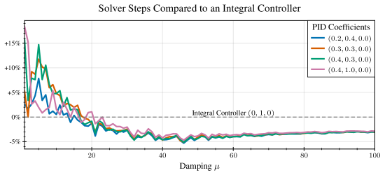
Figure 3: Solver steps required to solve one cycle of Van der Pol’s oscillator (see 1) with various PID coefficients compared to an integral controller.

A proportional-integral-derivative (PID) controller (Söderlind, 2002, 2003) can improve the performance of ODE solvers by avoiding unnecessary solver steps when the stiffness of the problem changes abruptly. Its decision about growing or shrinking the next solver time step is based on the last three error estimates instead of only the current one as in an integral controller. This way it can react more accurately when the stability requirements on the time step change quickly as in 1 and avoid rejected solver steps because of a too large step size as well as unnecessarily small solver steps. To gain some insight into the effect of PID control on the number of solver steps, we solve Van der Pol’s 1 for one cycle with various PID coefficients

and compare the number of solver steps to the steps that the same solver would take with an integral controller. By varying the damping strength $\mu$ and therefore also the stiffness of the problem, we can control how strongly the step size varies across one cycle. See 1 for the step sizes at $\mu=25$. For $\mu=0$, the limit cycle in phase space is a circle with very smooth step size behavior. With growing $\mu$, the limit cycle becomes more and more distorted and the variance in step size grows. The results in 3 show that there is a trade-off. For small variance in step size, i.e. $\mu<15$, the PID controllers even take more steps than an integral controller. Only after $\mu>25$ does PID control actually pay off with $3$ to $5\%$ in step savings over an integral controller. We conclude that PID control is a valuable tool for ODE problems that are difficult in the sense that the step size for an explicit method varies quickly and by at least two orders of magnitude. Given that the step size behavior of learned ODE models is quite benign in our experience, we recommend the simple integral controller by default for deep learning applications and to try a PID controller when the number of solver steps exceeds $100$ or a significant variation in step size has been observed.

References

- Bradbury et al. (2018) James Bradbury, Roy Frostig, Peter Hawkins, Matthew James Johnson, Chris Leary, Dougal Maclaurin, George Necula, Adam Paszke, Jake VanderPlas, Skye Wanderman-Milne, and Qiao Zhang. JAX: Composable transformations of Python+NumPy programs, 2018.
- Chen et al. (2018) Ricky T. Q. Chen, Yulia Rubanova, Jesse Bettencourt, and David K. Duvenaud. Neural Ordinary Differential Equations. In Neural Information Processing Systems, 2018.
- De Brouwer et al. (2019) Edward De Brouwer, Jaak Simm, Adam Arany, and Yves Moreau. GRU-ODE-Bayes: Continuous Modeling of Sporadically-Observed Time Series. In Neural Information Processing Systems, 2019.
- Dormand & Prince (1980) J. R. Dormand and P. J. Prince. A family of embedded Runge-Kutta formulae. Journal of Computational and Applied Mathematics, 6:19–26, 1980.
- Dupont et al. (2019) Emilien Dupont, Arnaud Doucet, and Yee Whye Teh. Augmented Neural ODEs. In Neural Information Processing Systems, 2019.
- Finlay et al. (2020) Chris Finlay, Jörn-Henrik Jacobsen, Levon Nurbekyan, and Adam M. Oberman. How to Train Your Neural ODE: The World of Jacobian and Kinetic Regularization. In International Conference on Machine Learning, 2020.
- Gander (2015) Martin J Gander. 50 Years of Time Parallel Time Integration. In Multiple Shooting and Time Domain Decomposition Methods, pp. 69–113. Springer, 2015.
- Gholami et al. (2019) Amir Gholami, Kurt Keutzer, and George Biros. ANODE: Unconditionally Accurate Memory-Efficient Gradients for Neural ODEs. In International Joint Conferences on Artificial Intelligence, 2019.
- Ghosh et al. (2020) Arnab Ghosh, Harkirat Singh Behl, Emilien Dupont, Philip H. S. Torr, and Vinay Namboodiri. STEER: Simple Temporal Regularization For Neural ODEs. In Neural Information Processing Systems. arXiv, 2020.
- Grathwohl et al. (2019) Will Grathwohl, Ricky T. Q. Chen, Jesse Bettencourt, Ilya Sutskever, and David Duvenaud. FFJORD: Free-Form Continuous Dynamics for Scalable Reversible Generative Models. In International Conference on Learning Representations, 2019.
- Kidger (2022) Patrick Kidger. On Neural Differential Equations. arXiv, 2022.
- Kidger et al. (2020) Patrick Kidger, James Morrill, James Foster, and Terry J. Lyons. Neural Controlled Differential Equations for Irregular Time Series. In Neural Information Processing Systems, 2020.
- Lienen & Günnemann (2022) Marten Lienen and Stephan Günnemann. Learning the Dynamics of Physical Systems from Sparse Observations with Finite Element Networks. In International Conference on Learning Representations, 2022.
- Ma et al. (2018) Yingbo Ma, Vaibhav Dixit, Mike Innes, Xingjian Guo, and Christopher Rackauckas. A Comparison of Automatic Differentiation and Continuous Sensitivity Analysis for Derivatives of Differential Equation Solutions. arXiv, 2018.
- Massaroli et al. (2020) Stefano Massaroli, Michael Poli, Jinkyoo Park, Atsushi Yamashita, and Hajime Asama. Dissecting Neural ODEs. In Neural Information Processing Systems, 2020.
- Norcliffe et al. (2021) Alexander Norcliffe, Cristian Bodnar, Ben Day, Jacob Moss, and Pietro Liò. Neural ODE Processes. In International Conference on Learning Representations, 2021.
- Ott et al. (2021) Katharina Ott, Prateek Katiyar, Philipp Hennig, and Michael Tiemann. ResNet After All: Neural ODEs and Their Numerical Solution. In International Conference on Learning Representations, 2021.
- Pal et al. (2021) Avik Pal, Yingbo Ma, Viral Shah, and Christopher Rackauckas. Opening the Blackbox: Accelerating Neural Differential Equations by Regularizing Internal Solver Heuristics. In International Conference on Machine Learning, 2021.
- Paszke et al. (2019) Adam Paszke, Sam Gross, Francisco Massa, Adam Lerer, James Bradbury, Gregory Chanan, Trevor Killeen, Zeming Lin, Natalia Gimelshein, Luca Antiga, Alban Desmaison, Andreas Köpf, Edward Yang, Zach DeVito, Martin Raison, Alykhan Tejani, Sasank Chilamkurthy, Benoit Steiner, Lu Fang, Junjie Bai, and Soumith Chintala. PyTorch: An Imperative Style, High-Performance Deep Learning Library. In Neural Information Processing Systems, 2019.
- Poli et al. (2019) Michael Poli, Stefano Massaroli, Junyoung Park, Atsushi Yamashita, Hajime Asama, and Jinkyoo Park. Graph Neural Ordinary Differential Equations. In Conference on Artificial Intelligence, Workshop on Deep Learning on Graphs: Methodologies and Applications, 2019.
- Poli et al. (2021) Michael Poli, Stefano Massaroli, Atsushi Yamashita, Hajime Asama, Jinkyoo Park, and Stefano Ermon. TorchDyn: Implicit Models and Neural Numerical Methods in PyTorch. In Neural Information Processing Systems, Workshop on Physical Reasoning and Inductive Biases for the Real World, 2021.
- Rackauckas et al. (2019) Chris Rackauckas, Mike Innes, Yingbo Ma, Jesse Bettencourt, Lyndon White, and Vaibhav Dixit. DiffEqFlux.jl - A Julia Library for Neural Differential Equations. arXiv, 2019.
- Rackauckas & Nie (2017) Christopher Rackauckas and Qing Nie. DifferentialEquations.jl – A Performant and Feature-Rich Ecosystem for Solving Differential Equations in Julia. Journal of Open Research Software, 5, 2017.
- Rubanova et al. (2019) Yulia Rubanova, Ricky T. Q. Chen, and David Duvenaud. Latent Ordinary Differential Equations for Irregularly-Sampled Time Series. In Neural Information Processing Systems, 2019.
- Söderlind (2002) Gustaf Söderlind. Automatic Control and Adaptive Time-Stepping. Numerical Algorithms, 31(1-4):281–310, 2002.
- Söderlind (2003) Gustaf Söderlind. Digital Filters in Adaptive Time-Stepping. ACM Transactions on Mathematical Software, 29:1–26, 2003.
- Tsitouras (2011) Ch Tsitouras. Runge–Kutta pairs of order 5 (4) satisfying only the first column simplifying assumption. Computers & Mathematics with Applications, 62(2):770–775, 2011.
- Xia et al. (2021) Hedi Xia, Vai Suliafu, Hangjie Ji, Tan M. Nguyen, Andrea L. Bertozzi, Stanley J. Osher, and Bao Wang. Heavy Ball Neural Ordinary Differential Equations. In Neural Information Processing Systems, 2021.
appendix.0appendix.0\EdefEscapeHexAppendixAppendix\hyper@anchorstartappendix.0\hyper@anchorend