Systematic KMTNet Planetary Anomaly Search, Paper VII: Complete Sample of $q<10^{-4}$ Planets from the First Four-Year Survey

Abstract

We present the analysis of seven microlensing planetary events with planet/host mass ratios $q<10^{-4}$: KMT-2017-BLG-1194, KMT-2017-BLG-0428, KMT-2019-BLG-1806, KMT-2017-BLG-1003, KMT-2019-BLG-1367, OGLE-2017-BLG-1806, and KMT-2016-BLG-1105. They were identified by applying the Korea Microlensing Telescope Network (KMTNet) AnomalyFinder algorithm to 2016–2019 KMTNet events. A Bayesian analysis indicates that all the lens systems consist of a cold super-Earth orbiting an M or K dwarf. Together with 17 previously published and three that will be published elsewhere, AnomalyFinder has found a total of 27 planets that have solutions with $q<10^{-4}$ from 2016–2019 KMTNet events, which lays the foundation for the first statistical analysis of the planetary mass-ratio function based on KMTNet data. By reviewing the 27 planets, we find that the missing planetary caustics problem in the KMTNet planetary sample has been solved by AnomalyFinder. We also find a desert of high-magnification planetary signals ($A\gtrsim 65$), and a follow-up project for KMTNet high-magnification events could detect at least two more $q<10^{-4}$ planets per year and form an independent statistical sample.

1 Introduction

Among current exoplanet detection methods, a unique capability of the gravitational microlensing technique (Mao & Paczynski, 1991; Gould & Loeb, 1992) is to detect low-mass ($M_{\rm planet}\lesssim 20M_{\oplus}$) cold planets beyond the snow line (Hayashi, 1981; Min et al., 2011), including Neptune-mass cold planets, which are common (Uranus and Neptune) in our Solar System and cold terrestrial planets, which are absent in our Solar System. Because the typical host stars of the microlensing planetary systems are M and K dwarfs, detections of $q<10^{-4}$ planets (where $q$ is the planet/host mass ratio) can reveal the abundance of low-mass cold planets and answer how common the outer solar system is.

However, since the first microlensing planet, which was detected in 2003 (Bond et al., 2004), the first 13 years of microlensing planetary detections only discovered six $q<10^{-4}$ planets and none of them had mass ratios below $4.4\times 10^{-5}$. The paucity of detected $q<10^{-4}$ planets led to important statistical implications for cold planets. Suzuki et al. (2016) analyzed 1474 microlensing events discovered by the Microlensing Observations in Astrophysics (MOA) survey (Sako et al., 2008) and formed a homogeneously selected sample including 22 planets. They found that the mass-ratio function of microlensing planets increases as $q$ decreases until a break at $q\sim 1.7\times 10^{-4}$, below which the planetary occurrence rate likely drops. This break suggests that the Neptune-mass planets are likely to be the most common of cold planets. However, the Suzuki et al. (2016) sample only contains two $q<10^{-4}$ and thus may be affected by small number statistics. To examine the existence of the break, a larger $q<10^{-4}$ sample is needed.

After its commissioning season in 2015, the new-generation microlensing survey, the Korea Microlensing Telescope Network (KMTNet, Kim et al. 2016), has been conducting near-continuous, wide-area, high-cadence surveys for $\sim 96~{}{\rm deg}^{2}$. The fields with cadences of $\Gamma\geq 2~{}{\rm hr}^{-1}$ are the KMTNet prime fields ($\sim 12~{}{\rm deg}^{2}$) and the other fields are the KMTNet sub-prime fields ($\sim 84~{}{\rm deg}^{2}$). Since 2016, the detections of $q<10^{-4}$ planets have been greatly increased in two ways, and the KMTNet data played a major or decisive role in all detections. First, more than ten $q<10^{-4}$ planets have been detected from by-eye searches, including three with $q<2\times 10^{-5}$ (Gould et al., 2020; Yee et al., 2021; Zang et al., 2021a). Second, Zang et al. (2021b, 2022a) developed the KMTNet AnomalyFinder algorithm to systematically search for planetary signals. This algorithm has been applied to the 2018 and 2019 KMTNet prime fields ($\Gamma\geq 2~{}{\rm hr}^{-1}$) and uncovered five new $q<10^{-4}$ planets (Zang et al., 2021b; Hwang et al., 2022; Gould et al., 2022). Moreover, the systematic search opens a window for a homogeneous large-scale KMTNet planetary sample. According to the experience from 2018 and 2019 KMTNet prime fields, we expect to detect $\gtrsim 20$ planets with $q<10^{-4}$ from 2016–2019 seasons. This will be an order of magnitude larger than the Suzuki et al. (2016) sample at $q<10^{-4}$.

To build the first KMTNet $q<10^{-4}$ statistical sample, we applied the KMTNet AnomalyFinder algorithm to the 2016–2019 KMTNet microlensing events. In this paper, we introduce seven new $q<10^{-4}$ events from this search. They are KMT-2017-BLG-1194, KMT-2017-BLG-0428, KMT-2019-BLG-1806/OGLE-2019-BLG-1250, KMT-2017-BLG-1003, KMT-2019-BLG-1367, OGLE-2017-BLG-1806/KMT-2017-BLG-1021, and KMT-2016-BLG-1105. Together with 17 already published and three that will be published elsewhere, the KMTNet AnomalyFinder algorithm found 27 events that can be fit by $q<10^{-4}$ models from 2016–2019 KMTNet data. However, whether a planet can be used for statistical studies requires further investigations, which is beyond the scope of this paper.

The paper is structured as follows. In Section 2, we briefly introduce the KMTNet AnomalyFinder algorithm and the procedure to form the $q<10^{-4}$ sample. In Sections 3, 4 and 5, we present the observations and the analysis of seven $q<10^{-4}$ events. Finally, we discuss the implications from the 2016–2019 KMTNet $q<10^{-4}$ planetary sample in Section 6.

2 The Basic of AnomalyFinder and the Procedure

Section 2 of Zang et al. (2021b) and Section 2 of Zang et al. (2022a) together introduced the KMTNet AnomalyFinder algorithm. The AnomalyFinder uses a Gould (1996) 2-dimensional grid of $(t_{0},t_{\rm eff})$ to search for and fit anomalies from the residuals to a point-source point-lens (PSPL, Paczyński 1986) model. Here $t_{0}$ is the time of maximum magnification, and $t_{\rm eff}$ is the effective timescale. For our search, the shortest $t_{\rm eff}$ is 0.05 days and the longest $t_{\rm eff}$ is 6.65 days. The parameters that evaluate the significance of a candidate anomaly are $\Delta\chi^{2}_{0}$ and $\Delta\chi^{2}_{\rm flat}$. See Equation (4) of Zang et al. (2021b) for their definitions. The criteria of $\Delta\chi^{2}_{0}$ and $\Delta\chi^{2}_{\rm flat}$ are the same as the criteria used in Zang et al. (2022a); Gould et al. (2022); Jung et al. (2022), with $\Delta\chi^{2}_{0}>200$, or $\Delta\chi^{2}_{0}>120$ and $\Delta\chi^{2}_{\rm flat}>60$ for the KMTNet prime-field events and $\Delta\chi^{2}_{0}>100$, or $\Delta\chi^{2}_{0}>60$ and $\Delta\chi^{2}_{\rm flat}>30$ for the KMTNet sub-prime-field events. Future statistical studies should use the same criteria. In addition, an anomaly is required to contain at least three successive points $\geq 2\sigma$ away from a PSPL model.

As a result, we found 464 and 608 candidate anomalies from 2016–2019 KMTNet prime-field and sub-prime-field events, respectively. We checked whether the data from other surveys are consistent with the KMTNet-based anomalies and cross-checked with C. Han’s modeling. We fitted all the $q<10^{-3}$ candidates with online data and found 13 new candidates with $q<2\times 10^{-4}$. Then, we conducted tender-loving care (TLC) re-reductions and re-fitted the 13 events. Of these, eight events unambiguously have $q<10^{-4}$, three events, KMT-2016-BLG-1307, KMT-2017-BLG-0849, and KMT-2017-BLG-1057, have $10^{-4}<q<2\times 10^{-4}$, and two events, KMT-2016-BLG-0625 (Shin et al. in prep) and OGLE-2017-BLG-0448/KMT-2017-BLG-0090 (Zhai et al. in prep), have ambiguous mass ratios at $10^{-5}\lesssim q\lesssim 10^{-3}$ and will be published elsewhere.

Among the eight unambiguous $q<10^{-4}$ events, one event, OGLE-2016-BLG-0007/MOA-2016-BLG-088/KMT-2016-BLG-1991, will be published elsewhere because it has the lowest-$q$ of this sample. We analyze and publish the remaining seven events in this paper. We note that the planetary signals of the seven events are not strong, although they are confirmed by at least two data sets. We thus further check whether the light curves have other similar anomalies, to exclude the possibility of unknown systematic errors. We applied the AnomalyFinder algorithm to the re-reduction data. For all of the seven events, besides the known planetary signals no anomaly with $\Delta\chi^{2}_{0}>20$ was detected. Therefore, the light curves of the seven events are stable and planetary signals are reliable.

3 Observations and Data Reductions

Table 1: Event Names, Alerts, Locations, and Cadences for the six planetary events

Event Name	Alert Date	${\rm RA}_{\rm J2000}$	${\rm Decl.}_{\rm J2000}$	$\ell$	$b$	$\Gamma({\rm hr}^{-1})$
KMT-2017-BLG-1194	Post Season	18:17:17.31	$-$25:19:26.18	+6.63	$-$4.34	0.4
KMT-2017-BLG-0428	Post Season	18:05:32.46	$-$28:29:25.01	+2.59	$-$3.55	4.0
KMT-2019-BLG-1806	26 Jul 2019	18:02:09.01	$-$29:24:53.60	+1.41	$-$3.35	1.0
OGLE-2019-BLG-1250						0.3
KMT-2017-BLG-1003	Post Season	17:41:38.76	$-$24:22:26.18	+3.42	+3.15	1.0
KMT-2019-BLG-1367	27 Jun 2019	18:09:53.12	$-$29:45:43.96	+1.93	$-$4.99	0.4
OGLE-2017-BLG-1806	14 Oct 2017	17:46:29.58	$-$24:16:20.17	+4.09	+2.26	0.3
KMT-2017-BLG-1021						1.0
KMT-2016-BLG-1105	Post Season	17:45:47.34	$-$26:15:58.93	+2.30	+1.16	1.0

Table 1 lists the basic observational information for the seven events, including event names, the first discovery date, the coordinates in the equatorial and galactic systems, and the nominal cadences ($\Gamma$). The seven planetary events were all identified by the KMTNet post-season EventFinder algorithm (Kim et al., 2018a). Of them, KMT-2019-BLG-1806/OGLE-2019-BLG-1250 and OGLE-2017-BLG-1806/KMT-2017-BLG-1021 were discovered by the KMTNet alert-finder system (Kim et al., 2018b) and the Early Warning System (Udalski et al., 1994; Udalski, 2003) of the Optical Gravitational Lensing Experiment (OGLE, Udalski et al. 2015), respectively, during their observational seasons. Hereafter, we designate KMT-2019-BLG-1806/OGLE-2019-BLG-1250 and OGLE-2017-BLG-1806/KMT-2017-BLG-1021 by their first-discovery name, KMT-2019-BLG-1806 and OGLE-2017-BLG-1806. During the 2019 observational season, the KMTNet alert-finder system also discovered KMT-2019-BLG-1367. In addition, OGLE observed the locations of KMT-2019-BLG-1367 and KMT-2016-BLG-1105 but did not alert them. We also include the OGLE data for these two events into the light-curve analysis, for which the OGLE data confirm the planetary signals found by the KMTNet. MOA did not issue alerts for any of the seven events, and there were no follow-up data to the best of our knowledge.

KMTNet conducted observations from three identical 1.6 m telescopes equipped with $4~{}{\rm deg}^{2}$ cameras in Chile (KMTC), South Africa (KMTS), and Australia (KMTA). OGLE took data using an 1.3m telescope with 1.4 ${\rm deg}^{2}$ field of view in Chile. For both surveys, most of the images were taken in the $I$ band, and a fraction of $V$-band images were acquired for source color measurements. Each KMTNet V-band data point was taken one minute before or after one KMTNet I-band data point of the same field.

The KMTNet and OGLE data used in the light-curve analysis were reduced using the custom photometry pipelines based on the difference imaging technique (Tomaney & Crotts, 1996; Alard & Lupton, 1998): pySIS (Albrow et al. 2009, Yang et al. in prep) for the KMTNet data, and Wozniak (2000) for the OGLE data. For each event, the KMTC data were additionally reduced using the pyDIA photometry pipeline (Albrow, 2017) to measure the source color. Except for OGLE-2017-BLG-1806 and KMT-2016-BLG-1105 whose sources are not located in any OGLE star catalog, the $I$-band magnitudes of the other five events reported in this paper have been calibrated to the standard $I$-band magnitude using the OGLE-III star catalog (Szymański et al., 2011).

4 Light-curve Analysis

4.1 Preamble

Because all seven events contain short-lived deviations from a PSPL model, we first introduce the common methods for the light-curve analysis. The PSPL model is described by three parameters, $t_{0}$, $u_{0}$, and $t_{\rm E}$, which respectively represent the time of lens-source closest approach, the closest lens-source projected separation normalized to the angular Einstein radius $\theta_{\rm E}$, and the Einstein timescale,

$$t_{\rm E}=\frac{\theta_{\rm E}}{\mu_{\rm rel}};\qquad\theta_{\rm E}=\sqrt{\kappa M_{\rm L}\pi_{\rm rel}},$$ (1)

where $\kappa\equiv\frac{4G}{c^{2}\mathrm{au}}\simeq 8.144\frac{{\rm mas}}{M_{\odot}}$, $M_{\rm L}$ is the lens mass, and $(\pi_{\rm rel},\mu_{\rm rel})$ are the lens-source relative (parallax, proper motion). In addition, for each data set $i$, we introduce two linear parameters, ($f_{{\rm S},i}$, $f_{{\rm B},i}$), to fit the flux of the source and any blend flux, respectively.

We search for binary-lens single-source (2L1S) models for each event. A 2L1S model requires four parameters in addition to the PSPL parameters, $(s,q,\alpha,\rho)$, which respectively denote the planet-host projected separation in units of $\theta_{\rm E}$, the planet/host mass ratio, the angle between the source trajectory and the binary axis, and the angular source radius $\theta_{*}$ scaled to $\theta_{\rm E}$, i.e., $\rho=\theta_{*}/\theta_{\rm E}$.

Although the final results need detailed numerical analysis, some of the 2L1S parameters can be estimated by heuristic analysis. A PSPL fit excluding the data points around the anomaly can yield the three PSPL parameters, $t_{0}$, $u_{0}$, and $t_{\rm E}$. If an anomaly occurred at $t_{\rm anom}$, the corresponding lens-source offset, $u_{\rm anom}$, and $\alpha$ can be estimated by

$$u_{\rm anom}=\sqrt{u_{0}^{2}+\left(\frac{t_{\rm anom}-t_{0}}{t_{\rm E}}\right)^{2}};\quad\left|\alpha\right|=\left|\sin^{-1}\frac{u_{0}}{u_{\rm anom}}\right|.$$ (2)

Because the planetary caustics are located at the position of $|s-s^{-1}|\sim u_{\rm anom}$, we obtain

$$s_{\pm}\sim\frac{\sqrt{u_{\rm anom}^{2}+4}\pm u_{\rm anom}}{2},$$ (3)

where $s=s_{+}$ and $s=s_{-}$ correspond to the major-image (quadrilateral) and the minor-image (triangular) planetary caustics, respectively. For two degenerate solutions with similar $q$ but different $s$, Ryu et al. (2022) suggested that the geometric mean of two solutions satisfies

$$s_{\rm mean}=s_{\pm}.$$ (4)

In addition, Zhang et al. (2022) suggested a slightly different formalism, and Zhang & Gaudi (2022) provided a theoretical treatment of it. For a dip-type planetary signal, Hwang et al. (2022) pointed out that the mass ratio can be estimated by

$$q=\left(\frac{\Delta t_{\rm dip}}{4t_{\rm E}}\right)^{2}\frac{s}{u_{0}}|\sin^{3}\alpha|,$$ (5)

where $\Delta t_{\rm dip}$ is the duration of the dip, and the accuracy of Equation (5) should be at a factor of $\sim 2$ level.

To find all the possible 2L1S models, we conduct two-phase grid searches for the parameters, ($\log s$, $\log q$, $\alpha$, $\rho$). In the first phase, we conduct a sparse grid, which consists of 21 values equally spaced between $-1.0\leq\log s\leq 1.0$, 20 values equally spaced between $0^{\circ}\leq\alpha<360^{\circ}$, 61 values equally spaced between $-6.0\leq\log q\leq 0.0$ and five values equally spaced between $-3.5\leq\log\rho\leq-1.5$. We use a code based on the advanced contour integration code (Bozza, 2010; Bozza et al., 2018), VBBinaryLensing to compute the 2L1S magnification. For each grid point, we search for the minimum $\chi^{2}$ by Markov chain Monte Carlo (MCMC) $\chi^{2}$ minimization using the emcee ensemble sampler (Foreman-Mackey et al., 2013), with fixed ($\log q$, $\log s$) and free ($t_{0},u_{0},t_{\rm E},\rho,\alpha$). In the second phase, we conduct a denser ($\log s$, $\log q$, $\alpha$, $\rho$) grid search around each local minimum (e.g., Zang et al. 2022b). Finally, we refine the best-fit models by MCMC with all parameters free.

For degenerate solutions, Yang et al. (2022) suggested that the phase-space factors can be used to weight the probability of each solution. We follow the procedures of Yang et al. (2022) and first calculate the covariance matrix, $\bm{C}$, of ($\log s,\log q,\alpha$) from the MCMC chain. Then, the phase-space factor is

$$p=\sqrt{{\rm det}(\bm{C})}.$$ (6)

Because whether a planet and its individual solutions can be used for statistical studies requires further investigations, we provide the phase-space factors for the event with multiple solutions but do not use them to weight or reject solutions.

We also investigate whether the inclusion of two high-order effects can improve the fit. The first is the microlensing parallax effect (Gould, 1992, 2000, 2004), which is due to the Earth’s orbital acceleration around the Sun. We fit it by two parameters, $\pi_{\rm E,N}$ and $\pi_{\rm E,E}$, which are the north and east components of the microlensing parallax vector $\bm{\pi}_{\rm E}$ in equatorial coordinates,

$$\bm{\pi}_{\rm E}\equiv\frac{\pi_{\rm rel}}{\theta_{\rm E}}\frac{\bm{\mu}_{\rm rel}}{\mu_{\rm rel}}.$$ (7)

We also fit the $u_{0}>0$ and $u_{0}<0$ solutions to consider the “ecliptic degeneracy” (Jiang et al., 2004; Poindexter et al., 2005). For four cases in this paper, the parallax contours take the form of elongated ellipses, so we report the constraints on the minor axes of the error ellipse, ($\pi_{\rm E,\parallel}$), which is approximately parallel with the direction of the Earth’s acceleration. For the major axes of the parallax contours, $\pi_{\rm E,\bot}\sim\pi_{\rm E,N}$, we only report it when the constraint is useful.

The second effect is the lens orbital motion effect (Batista et al., 2011; Skowron et al., 2011), and we fit it by the parameter $\vec{\gamma}=\left(\frac{ds/dt}{s},\frac{d\alpha}{dt}\right)$, where $ds/dt$ and $d\alpha/dt$ represent the instantaneous changes in the separation and orientation of the two components defined at $t_{0}$, respectively. To exclude unbound systems, we restrict the MCMC trials to $\beta<1.0$. Here $\beta$ is the absolute value of the ratio of projected kinetic to potential energy (An et al., 2002; Dong et al., 2009),

$$\beta\equiv\left|\frac{{\rm KE}_{\perp}}{{\rm PE}_{\perp}}\right|=\frac{\kappa M_{\odot}{\rm yr}^{2}}{8\pi^{2}}\frac{{\pi}_{\rm E}}{\theta_{\rm E}}\gamma^{2}\left(\frac{s}{{\pi}_{\rm E}+\pi_{\rm S}/\theta_{\rm E}}\right)^{3},$$ (8)

and where $\pi_{\rm S}$ is the source parallax estimated by the mean distance to red clump stars in the direction of each event (Nataf et al., 2013).

4.2 “Dip” Anomalies

4.2.1 KMT-2017-BLG-1194

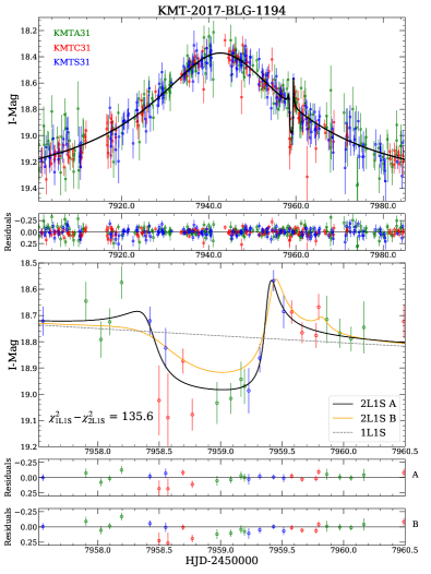
Figure 1: The observed data and the 2L1S (the black and orange solid lines) and 1L1S models (the grey dashed line) for KMT-2017-BLG-1194. The data taken from different data sets are shown with different colors. The bottom panels show a close-up of the dip-type planetary signal and the residuals to the 2L1S models.

Table 2: 2L1S Parameters for KMT-2017-BLG-1194

Parameter	A	B
$\chi^{2}$/dof	928.0/928	950.6/928
$t_{0}$ (${\rm HJD}^{\prime}$)	$7942.66\pm 0.13$	$7942.59\pm 0.13$
$u_{0}$	$0.256\pm 0.018$	$0.246\pm 0.011$
$t_{\rm E}$ (days)	$47.0\pm 2.5$	$47.9\pm 1.7$
$\rho(10^{-3})$	$<2.6$	$<1.4$
$\alpha$ (rad)	$2.505\pm 0.013$	$2.515\pm 0.011$
$s$	$0.8063\pm 0.0103$	$0.8055\pm 0.0065$
$\log q$	$-4.582\pm 0.058$	$-4.585\pm 0.074$
$I_{\rm S,OGLE}$	$20.28\pm 0.08$	$20.34\pm 0.06$

Figure 1 shows the observed data together with the best-fit PSPL and 2L1S models for KMT-2017-BLG-1194. There is a dip centered on ${\rm HJD}^{\prime}\sim 7958.9~{}({\rm HJD}^{\prime}={\rm HJD}-2450000)$ , i.e., $t_{\rm anom}\sim 7958.9$, with a duration of $\Delta t_{\rm dip}\sim 1.05$ days. The dip and the ridge around the dip are covered by three KMTNet sites, so the anomaly is secure. A PSPL fit yields ($t_{0}$, $u_{0}$, $t_{\rm E}$) = (7942.7, 0.26, 46), and using the heuristic formalism of Section 4.1, we obtain

$$\alpha\sim 143.5^{\circ};\quad s=s_{-}\sim 0.807;\quad\log q\sim-4.68.$$ (9)

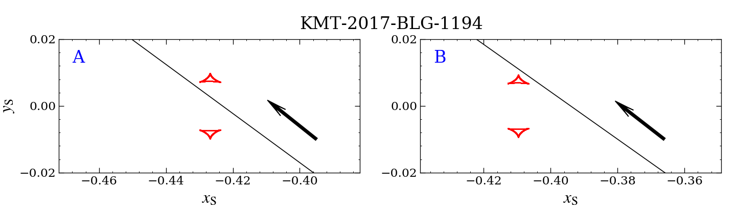
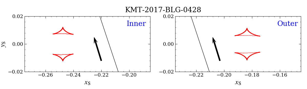
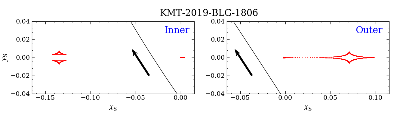
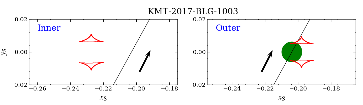
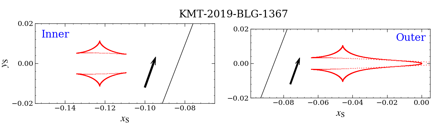
Figure 2: Geometries of the five “dip” planetary events. In each panel, the red lines represent the caustic, the black solid line represents the source trajectory, and the line with an arrow indicates the direction of the source motion. For the outer solution of KMT-2017-BLG-1003, $\rho$ is constrained at the $>3\sigma$ level, so the radius of the green dot represents the source radius. For other solutions, $\rho$ only has weak constraints with $<3\sigma$, so their source radii are not shown.

The grid search yields one solution. Its parameters are presented in Table 2 and are in good agreement with the heuristic estimates. The top left panel of Figure 2 displays the caustic structure and the source trajectory, for which the two minor-image planetary caustics are located on both sides of the source trajectory. We label the solution as the solution “A”. To further investigate the parameter space and check whether the event has the inner/outer solutions (Gaudi & Gould, 1997), for which the source passes inside (the “Inner” solution) the two planetary caustics (closer to the central caustic) or outside (the “Outer” solution), we follow the procedures of Hwang et al. (2018a). First, we conduct a “hotter” MCMC with the error bar inflated by a factor of $\sqrt{3.0}$. Second, we make a scatter plot of $\log q$ versus $\Delta\xi$ from the “hotter” MCMC chain. Here $\Delta\xi$ represents the offset between the source and the planetary caustic as the source crosses the binary axis,

$$\Delta\xi=u_{0}\csc(\alpha)-(s-s^{-1}).$$ (10)

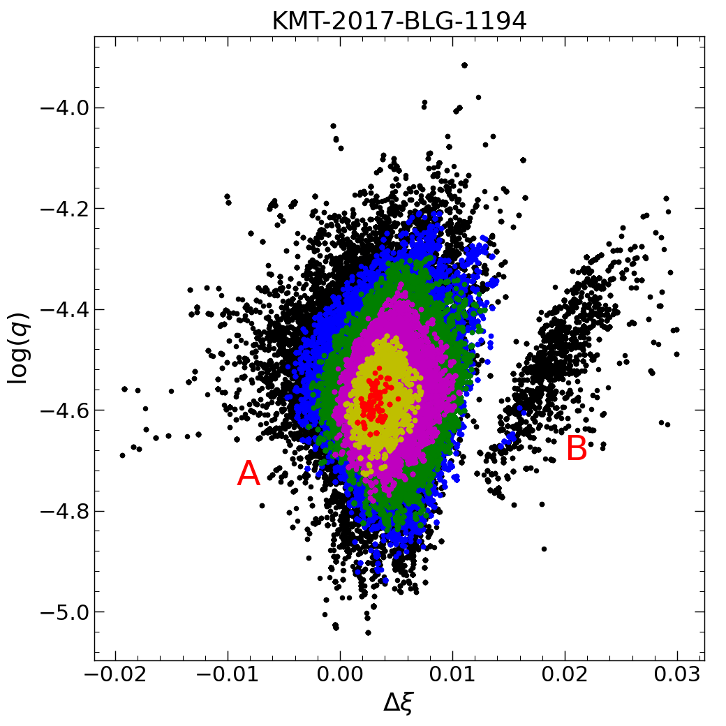
Figure 3: Scatter plot of $\log q$ vs. $\Delta\xi$ for KMT-2017-BLG-1194, where $\Delta\xi=u_{0}\csc(\alpha)-(s-s^{-1})$ represents the offset between the source and the center of the planetary caustic at the moment that the source crosses the binary axis. The distribution is derived by inflating the error bars by a factor of $\sqrt{3}$ and then multiplying the resulting $\chi^{2}$ by 3 for the plot. Red, yellow, magenta, green, blue and black colors represent $\Delta\chi^{2}<2\times(1,4,9,16,25,\infty)$. “A” and “B” represent two local minima and the corresponding parameters are given in Table 2.

The resulting scatter plot is shown in Figure 3, from which we find another local minimum at $\Delta\xi\sim 0.02$. We label this solution as the “B” solution. As shown in the top right panel of Figure 2, the “B” solution corresponds to the “Inner” solution. Its parameters from MCMC are given in Table 2 and it is disfavored by $\Delta\chi^{2}=22.6$ compared to the “A” solution. In Figure 1, the “B” solution cannot fit the anomaly well and all three KMTNet data sets contribute to the $\Delta\chi^{2}$. The ratio of the phase-space factors is $p_{\rm A}:p_{\rm B}=1:0.54$, which also prefers the “A” solution. Thus, we exclude the “B” solution. In addition, the models, which have the geometry of the “Outer” solution, do not form a local minimum and are disfavored by $\Delta\chi^{2}>60$ compared to the “A” solution.

For the “A” solution a point-source model is consistent within $1\sigma$ and the $3\sigma$ upper limit is $\rho<0.0026$. The inclusion of higher-order effects yields a constraint on $\pi_{\rm E,\parallel}$, and with the other 2L1S parameters being almost unchanged. We obtain $\pi_{\rm E,\parallel}=-0.18\pm 0.35$ and adopt the constraints on ${\pi}_{\rm E}$ and $\rho$ in the Bayesian analysis of Section 5. This is a new microlensing planet with $q\sim 2.62\times 10^{-5}$; i.e., about nine times the Earth/Sun mass ratio.

4.2.2 KMT-2017-BLG-0428

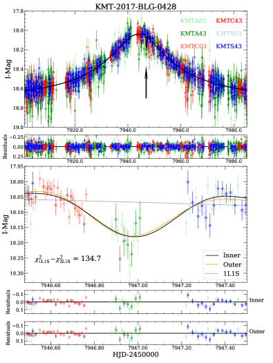
Figure 4: The observed data and models for KMT-2017-BLG-0428. The symbols are similar to those in Figure 1. In the top panel, the black arrow indicates the position of the planetary signal.

Table 3: 2L1S Parameters for KMT-2017-BLG-0428

Parameter	Inner	Outer
$\chi^{2}$/dof	9952.0/9952	9952.1/9952
$t_{0}$ (${\rm HJD}^{\prime}$)	$7943.976\pm 0.030$	$7943.978\pm 0.031$
$u_{0}$	$0.205\pm 0.009$	$0.205\pm 0.009$
$t_{\rm E}$ (days)	$44.4\pm 1.5$	$44.3\pm 1.5$
$\rho(10^{-3})$	$<6.4$	$<6.1$
$\alpha$ (rad)	$1.890\pm 0.005$	$1.889\pm 0.005$
$s$	$0.8819\pm 0.0044$	$0.9146\pm 0.0050$
$\log q$	$-4.295\pm 0.072$	$-4.302\pm 0.075$
$I_{\rm S,OGLE}$	$20.43\pm 0.05$	$20.43\pm 0.05$

Figure 4 shows a $\Delta I\sim 0.12$ mag dip at $t_{\rm anom}\sim 7947.00$, with a duration of $\Delta t_{\rm dip}\sim 0.74$ days. The dip is defined by the KMTA and KMTC data, and the subtle ridges are supported by both the KMTC and KMTS data. These data were taken in good seeing ($1.^{\prime\prime}4$–$2.^{\prime\prime}5$) and the anomaly does not correlate with seeing, sky background or airmass. In addition, Ishitani Silva et al. (2022) found that the KMTA data show systematic errors and excluded them from the analysis. In that case, the KMTA data exhibit similar residuals from one-night data in many places of the light curves. For the present case, the anomaly is mainly covered by the KMTA data, but as presented in Section 2, there is no similar deviation in other places of the light curves. We also carefully checked the KMTA data but did not find any similar residuals. Hence, the anomaly is secure. Applying the heuristic formalism of Section 4.1, we obtain

$$\alpha\sim 108.4^{\circ};\quad s=s_{-}\sim 0.898;\quad\log q\sim-4.19.$$ (11)

The 2L1S modeling yields two degenerate solutions with $\Delta\chi^{2}=0.1$. As shown in Figure 2, the two solutions are subjected to the inner/outer degeneracy. Their parameters are given in Table 3, for which $\alpha$ and $q$ are consistent with Equation (11). For $s$, we note that the geometric mean of the two solutions, $s_{\rm mean}=0.898\pm 0.005$, is in good agreement with Equation (11) and thus the formalism of Ryu et al. (2022). In addition, the observed data only provide a $3\sigma$ upper limit on $\rho$, and a point-source model is consistent within $1\sigma$. The ratio of the phase-space factors is $p_{\rm inner}:p_{\rm outer}=0.78:1$.

With high-order effects, we find that the $\chi^{2}$ improvement is $\sim 3$ and other parameters are almost the same. The constraint of ${\pi}_{\rm E}$, $\pi_{\rm E,\parallel}=-0.35\pm 0.26$, will be used in the Bayesian analysis. This is a microlensing planet with a Neptune/Sun mass ratio.

4.2.3 KMT-2019-BLG-1806

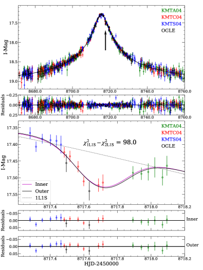
Figure 5: The observed data and models for KMT-2019-BLG-1806. The symbols are similar to those in Figure 1. In the top panel, the black arrow indicates the position of the planetary signal.

Table 4: 2L1S Parameters KMT-2019-BLG-1806

Parameter	Inner		Outer
	$u_{0}>0$	$u_{0}<0$	$u_{0}>0$	$u_{0}<0$
$\chi^{2}$/dof	3132.5/3132	3132.9/3132	3132.2/3132	3131.8/3132
$t_{0}$ (${\rm HJD}^{\prime}$)	$8715.452\pm 0.015$	$8715.451\pm 0.015$	$8715.453\pm 0.014$	$8715.453\pm 0.015$
$u_{0}$	$0.0260\pm 0.0017$	$-0.0251\pm 0.0020$	$0.0257\pm 0.0016$	$-0.0255\pm 0.0015$
$t_{\rm E}$ (days)	$132.8\pm 8.1$	$138.5\pm 10.8$	$134.1\pm 7.9$	$135.6\pm 7.9$
$\rho(10^{-3})$	$<1.8$	$<1.8$	$<1.9$	$<1.7$
$\alpha$ (rad)	$2.150\pm 0.008$	$-2.147\pm 0.008$	$2.151\pm 0.009$	$-2.148\pm 0.008$
$s$	$0.9377\pm 0.0069$	$0.9383\pm 0.0073$	$1.0339\pm 0.0084$	$1.0352\pm 0.0085$
$\log q$	$-4.724\pm 0.117$	$-4.734\pm 0.109$	$-4.717\pm 0.117$	$-4.714\pm 0.116$
$\pi_{\rm E,N}$	$-0.055\pm 0.150$	$-0.066\pm 0.161$	$-0.060\pm 0.156$	$-0.019\pm 0.160$
$\pi_{\rm E,E}$	$-0.058\pm 0.017$	$-0.059\pm 0.014$	$-0.057\pm 0.017$	$-0.060\pm 0.013$
$I_{\rm S}$	$21.33\pm 0.07$	$21.37\pm 0.09$	$21.34\pm 0.07$	$21.35\pm 0.07$

The anomaly of KMT-2019-BLG-1806 is also a dip, as shown in Figure 5. The dip has $\Delta t_{\rm dip}\sim 0.6$ days and centers on $t_{\rm anom}\sim 8717.72$. The dip is defined by the KMTC data and the two contemporaneous OGLE points, which were taken in good seeing ($1.^{\prime\prime}1$–$2.^{\prime\prime}4$) and low sky background. Hence, the anomaly is secure. Applying the heuristic formalism of Section 4.1, we obtain

$$\alpha\sim 123.3^{\circ};\quad s=s_{-}\sim 0.985;\quad\log q\sim-4.56.$$ (12)

In addition, given the Einstein timescale ($t_{\rm E}\sim 135$ days), we expect that ${\pi}_{\rm E}$ should be either measured or strongly constrained.

The 2L1S modeling also finds a pair of inner/outer solutions and combined the $u_{0}>0$ and $u_{0}<0$ degeneracy there are four solutions in total. See Table 4 for their parameters. The inclusion of ${\pi}_{\rm E}$ improves the fits by $\Delta\chi^{2}=31$, and all four data sets contribute to the improvement, so the parallax signal is reliable. The angle of the minor axis of the parallax ellipse (north through east) is $\psi=82.0^{\circ}$ and $\psi=82.5^{\circ}$ for the $u_{0}>0$ and $u_{0}<0$ solutions, respectively. $\pi_{\rm E,\parallel}=0.06\pm 0.01$, and $\pi_{\rm E,\bot}$ is constrained to be $\sigma(\pi_{\rm E,\bot})\sim 0.2$. We obtain $s_{\rm mean}=0.985\pm 0.008$, $\alpha=123.1\pm 0.5$, and $\log q\sim-4.72$, in good agreement with Equation (12). The ratio of the phase-space factors is $p_{\rm inner}:p_{\rm outer}=0.80:1$.

We find that the inclusion of the lens orbital motion effect only improves the fit by $\Delta\chi^{2}<1$ for 2 degree-of-freedom and is not correlated with ${\pi}_{\rm E}$, so we exclude the lens orbital motion effect. With $q\sim 1.9\times 10^{-5}$, this new planet is the fifth robust $q<2\times 10^{-5}$ microlensing planet.

4.2.4 KMT-2017-BLG-1003

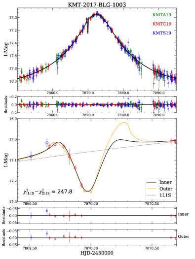
Figure 6: Light curve and models for KMT-2017-BLG-1003. The symbols are similar to those in Figure 1.

Table 5: 2L1S Parameters for KMT-2017-BLG-1003

Parameter	Inner	Outer
$\chi^{2}$/dof	2433.2/2433	2433.0/2433
$t_{0}$ (${\rm HJD}^{\prime}$)	$7872.484\pm 0.020$	$7872.482\pm 0.020$
$u_{0}$	$0.179\pm 0.005$	$0.179\pm 0.005$
$t_{\rm E}$ (days)	$25.65\pm 0.57$	$25.66\pm 0.59$
$\rho(10^{-3})$	$<6.7$	$5.22\pm 1.16$
$\alpha$ (rad)	$1.073\pm 0.006$	$1.072\pm 0.006$
$s$	$0.8889\pm 0.0043$	$0.9096\pm 0.0045$
$\log q$	$-4.260\pm 0.152$	$-4.373\pm 0.144$
$I_{\rm S,OGLE}$	$19.30\pm 0.04$	$19.30\pm 0.04$

Figure 6 shows the light curve and the best-fit models for KMT-2017-BLG-1003. The KMTC data show a sudden dip and the ridge is confirmed by the KMTC and KMTS data. These data were taken in good seeing ($1.^{\prime\prime}2$–$2.^{\prime\prime}2$) and low sky background, so the anomaly is of astrophysical origin. Although the end of the dip is not covered, the KMTC point at ${\rm HJD}^{\prime}=7870.66$ indicates $\Delta t_{\rm dip}<0.85$ days, which yields

$$\alpha\sim 61.3^{\circ};\quad s=s_{-}\sim 0.903;\quad\log q<-3.6.$$ (13)

The numerical analysis yields a pair of inner/outer solutions, and Table 5 lists their parameters. As shown in Figure 2, the “Outer” solution has caustic crossings, so its $\rho$ is measured at the $4.5\sigma$ level. For the “Inner” solution, a point-source model is consistent within $2\sigma$. We note that the geometric mean of $s$, $s_{\rm mean}=0.899\pm 0.004$, which is slightly different from $s_{-}$ by $1\sigma$. This indicates that the prediction of Ryu et al. (2022) might be imperfect for minor-image anomalies with finite-source effects or incomplete coverage. The ratio of the phase-space factors is $p_{\rm inner}:p_{\rm outer}=0.80:1$.

With high-order effects, the $\chi^{2}$ improvement is 1.7. Although this event is shorter than the first two events, ${\pi}_{\rm E}$ is better constrained due to the about one magnitude brighter data, with $\pi_{\rm E,\parallel}=-0.11\pm 0.15$. This is another Neptune/Sun mass-ratio planet.

4.2.5 KMT-2019-BLG-1367

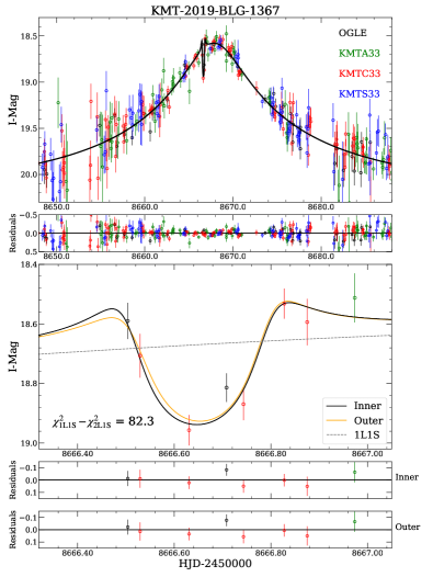
Figure 7: Light curve and models for KMT-2019-BLG-1367. The symbols are similar to those in Figure 1.

Table 6: 2L1S Parameters for KMT-2019-BLG-1367

Parameter	Inner	Outer
$\chi^{2}$/dof	1404.0/1404	1404.2/1404
$t_{0}$ (${\rm HJD}^{\prime}$)	$8667.883\pm 0.051$	$8667.884\pm 0.048$
$u_{0}$	$0.083\pm 0.009$	$0.082\pm 0.009$
$t_{\rm E}$ (days)	$39.3\pm 3.8$	$39.8\pm 4.0$
$\rho(10^{-3})$	$<5.3$	$<5.6$
$\alpha$ (rad)	$1.208\pm 0.016$	$1.207\pm 0.016$
$s$	$0.9389\pm 0.0066$	$0.9763\pm 0.0070$
$\log q$	$-4.303\pm 0.118$	$-4.298\pm 0.103$
$I_{\rm S,OGLE}$	$21.46\pm 0.13$	$21.48\pm 0.13$

Figure 7 shows a dip 1.2 days before the peak of an otherwise normal PSPL event, with a duration of $\Delta t_{\rm dip}\sim 0.35$ days. The dip-type anomaly is covered by the KMTC data and one contemporaneous OGLE point, and these data were taken in good seeing ($<2.^{\prime\prime}0$) and low sky background. Therefore, the anomaly is secure. Applying the heuristic formalism of Section 4.1, we obtain

$$\alpha\sim 69.5^{\circ};\quad s=s_{-}\sim 0.957;\quad\log q\sim-4.33.$$ (14)

The 2L1S modeling also yields a pair of inner/outer solutions, with $\Delta\chi^{2}=0.2$. The resulting solutions are given in Table 6 and Figure 2. A point-source model is consistent within $1\sigma$ and the $3\sigma$ upper limit is $\rho<0.0056$, so we expect that the Ryu et al. (2022) formula is applicable. We obtain $s_{\rm mean}=0.957\pm 0.007$, in good agreement with $s_{-}$. The ratio of the phase-space factors is $p_{\rm inner}:p_{\rm outer}=0.82:1$. We find that the inclusion of higher-order effects only improves the fitting by $\Delta\chi^{2}<1$ and the $1\sigma$ uncertainty of parallax is $>0.9$ at all directions, so the constraint on ${\pi}_{\rm E}$ is not useful for the Bayesian analysis. This is another planet with a Neptune/Sun mass ratio.

4.3 “Bump” Anomalies

For bump-type planetary signals, we also check whether the observed data can be fitted by a single-lens binary-source (1L2S) model (Gaudi, 1998) because it can also produce such anomalies (e.g., Hwang et al. 2013; Jung et al. 2017; Rota et al. 2021). For a 1L2S model, its magnification, $A_{\lambda}$, is the superposition of magnifications for two single-lens single-source (1L1S) models,

$$A_{\lambda}=\frac{A_{1}f_{1,\lambda}+A_{2}f_{2,\lambda}}{f_{1,\lambda}+f_{2,\lambda}}=\frac{A_{1}+q_{f,\lambda}A_{2}}{1+q_{f,\lambda}};\quad q_{f,\lambda}\equiv\frac{f_{2,\lambda}}{f_{1,\lambda}},$$ (15)

where $f_{{\rm i},\lambda}$ is the source flux at wavelength $\lambda$, and $i=1$ and $i=2$ correspond to the primary and the secondary sources, respectively.

4.3.1 OGLE-2017-BLG-1806

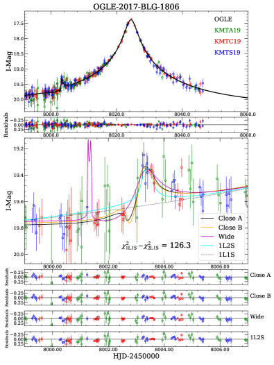
Figure 8: Light curve and models for OGLE-2017-BLG-1806. The symbols are similar to those in Figure 1. Different with the previous four events, the anomaly is bump-type, so the best-fit 1L2S model is provided.

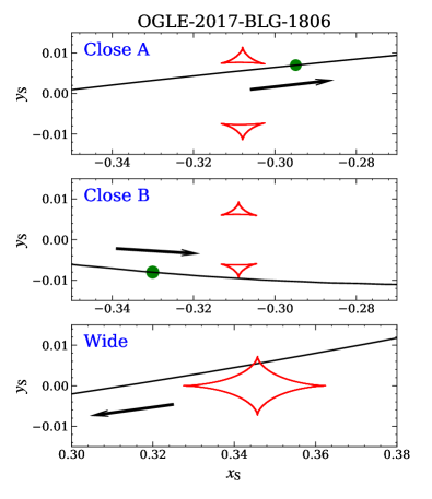
Figure 9: Geometries of OGLE-2017-BLG-1806. The symbols are similar to those in Figure 2. For the two “Close” solutions, $\rho$ is constrained at the $>3\sigma$ level, so the radius of the two green dots represent the source radius. For the “Wide” solution, $\rho$ only has weak constraints with $<3\sigma$, so its source radius is not shown.

Table 7: 2L1S Parameters for OGLE-2017-BLG-1806

Parameter	Close A		Close B		Wide
	$u_{0}>0$	$u_{0}<0$	$u_{0}>0$	$u_{0}<0$	$u_{0}>0$	$u_{0}<0$
$\chi^{2}$/dof	1650.9/1651	1650.7/1651	1664.8/1651	1665.5/1651	1659.1/1651	1659.0/1651
$t_{0}$ (${\rm HJD}^{\prime}$)	$8024.392\pm 0.020$	$8024.393\pm 0.019$	$8024.388\pm 0.020$	$8024.388\pm 0.020$	$8024.388\pm 0.020$	$8024.379\pm 0.020$
$u_{0}$	$0.0249\pm 0.0016$	$-0.0260\pm 0.0016$	$0.0256\pm 0.0020$	$-0.0253\pm 0.0019$	$0.0269\pm 0.0018$	$-0.0257\pm 0.0017$
$t_{\rm E}$ (days)	$69.4\pm 4.0$	$66.8\pm 3.9$	$69.4\pm 4.8$	$69.6\pm 4.6$	$64.5\pm 3.9$	$67.0\pm 3.9$
$\rho(10^{-3})$	$1.74_{-0.44}^{+0.78}$	$1.83_{-0.50}^{+0.80}$	$1.50_{-0.47}^{+0.62}$	$1.65_{-0.50}^{+0.67}$	$<2.8$	$<2.4$
$\alpha$ (rad)	$0.001\pm 0.034$	$-0.002\pm 0.037$	$0.267\pm 0.066$	$-0.263\pm 0.068$	$3.121\pm 0.034$	$-3.121\pm 0.036$
$s$	$0.8609\pm 0.0069$	$0.8566\pm 0.0075$	$0.8592\pm 0.0085$	$0.8601\pm 0.0080$	$1.1900\pm 0.0117$	$1.1806\pm 0.0108$
$\log q$	$-4.392\pm 0.180$	$-4.352\pm 0.171$	$-4.766\pm 0.220$	$-4.768\pm 0.209$	$-4.317\pm 0.126$	$-4.441\pm 0.168$
$\pi_{\rm E,N}$	$-0.278\pm 0.148$	$0.292\pm 0.170$	$0.774\pm 0.315$	$-0.756\pm 0.326$	$-0.535\pm 0.175$	$0.504\pm 0.170$
$\pi_{\rm E,E}$	$0.105\pm 0.056$	$0.144\pm 0.058$	$0.157\pm 0.070$	$0.124\pm 0.059$	$0.120\pm 0.065$	$0.133\pm 0.056$
$I_{\rm S,KMTC}$	$21.12\pm 0.07$	$21.07\pm 0.07$	$21.10\pm 0.08$	$21.10\pm 0.08$	$21.03\pm 0.07$	$21.08\pm 0.07$

Table 8: 1L2S Parameters for OGLE-2017-BLG-1806 and KMT-2016-BLG-1105

Parameters	OGLE-2017-BLG-1806		KMT-2016-BLG-1105
	$u_{0}>0$	$u_{0}<0$
$\chi^{2}$/dof	$1682.0/1651$	$1681.4/1651$	$2298.7/2288$
$t_{0,1}$ (${\rm HJD}^{\prime}$)	$8024.383\pm 0.020$	$8024.381\pm 0.020$	$7555.972\pm 0.094$
$t_{0,2}$ (${\rm HJD}^{\prime}$)	$8003.876\pm 0.274$	$8003.913\pm 0.253$	$7547.890\pm 0.021$
$u_{0,1}$	$0.0288\pm 0.0023$	$-0.0282\pm 0.0019$	$0.143\pm 0.022$
$u_{0,2}$	$0.003\pm 0.025$	$-0.004\pm 0.023$	$0.0001\pm 0.0007$
$t_{\rm E}$ (days)	$61.2\pm 4.3$	$62.2\pm 3.5$	$44.9\pm 5.8$
$\rho_{2}$ ($10^{-3}$)	$<7.3$	$<7.0$	$<3.3$
$q_{f,I}(10^{-3})$	$2.76\pm 0.76$	$2.63\pm 0.74$	$1.98\pm 0.48$
$\pi_{\rm E,N}$	$0.041\pm 0.388$	$0.059\pm 0.355$	…
$\pi_{\rm E,E}$	$0.111\pm 0.072$	$0.117\pm 0.063$	…
$I_{\rm S,KMTC}$	$20.96\pm 0.09$	$20.98\pm 0.07$	$21.31\pm 0.18$

As shown in Figure 8, the light curve of OGLE-2017-BLG-1806 exhibits a bump centered on $t_{\rm anom}\sim 8003.5$, defined by the KMTC and KMTS data. Except for two KMTS points, all the KMTC and KMTS data during $8003<{\rm HJD}^{\prime}<8005$ were taken in good seeing ($<2.^{\prime\prime}2$) and low sky background. In addition, most of the data before the bump ($8000<{\rm HJD}^{\prime}<8003$) are fainter than the 1L1S model. Hence, the signal is secure. Because both the major-image and the two minor-image planetary caustics can produce a bump-type anomaly (e.g., Wang et al. 2022), we obtain

$$\alpha\sim 184.6^{\circ}~{}{\rm for}~{}s_{+}\sim 1.15;\quad\alpha\sim 4.6^{\circ}~{}{\rm for}~{}s_{-}\sim 0.86.$$ (16)

The grid search returns three local minima, and their caustic structures are given in Figure 9. As expected, the three solutions respectively correspond to sources crossing a major-image (quadrilateral) planetary caustic and two minor-image (triangular) planetary caustics. We label the three solutions as “Close A”, “Close B”, and “Wide”, respectively, and their parameters are presented in Table 7.

The “Close A” solution provides the best fit to the observed data, and the “Close B” and “Wide” solutions are disfavored by $\Delta\chi^{2}=14.1$ and 8.3, respectively. We find that the inclusion of the parallax effect improves the fit by $\Delta\chi^{2}=$ 7.8, 20.4, and 11.1 for the “Close A”, “Close B”, and “Wide” solutions, respectively, and during the anomaly region ($7998<{\rm HJD}^{\prime}<8008$), $\Delta\chi^{2}=$2.2, 22.3, and 6.8. With the anomaly removed, fitting the data by a 1L1S model yields a similar constraint on $\pi_{\rm E,\parallel}$ and a weaker constraint on $\pi_{\rm E,\perp}$, with $\sigma(\pi_{\rm E,\bot})\sim 0.5$. Thus, the long planetary signal plays an important role in improving the constraint on $\pi_{\rm E,\bot}$ and reduces the $\chi^{2}$ differences between the three solutions.

The ratio of the phase-space factors is $p_{\rm CloseA}:p_{\rm CloseB}:p_{\rm Wide}=1:0.95:0.61$. For the “Close A”, and “Close B” solutions, the bump was produced by a caustic crossing, so $\rho$ is constrained at the $>3\sigma$ level. For the “Wide” solution, the bump was a result of a cusp approach. Although the “Wide” solution has caustic crossing features, due to the lack of data during the crossing, a point-source model is consistent within $1\sigma$.

The 1L2S model is disfavored by $\Delta\chi^{2}=30.7$ compared to the “Close A” solution, and the 1L2S parameters are shown in Table 8. Although the 1L2S model fits the bump well, it provides a worse fit to the observed data before the bump, during which most of the data from the three KMTNet sites are fainter than the 1L2S model. Hence, the 1L2S model is rejected. We find that the lens orbital motion effect is not detectable ($\Delta\chi^{2}<0.5$), so we adopt the parameters with the microlensing parallax effect as our final results.

4.3.2 KMT-2016-BLG-1105

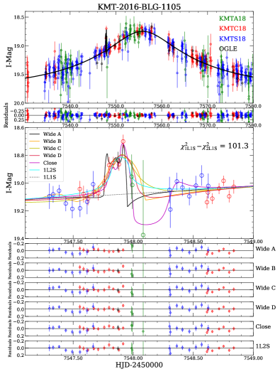
Figure 10: Light curve and models for KMT-2016-BLG-1105. The symbols are similar to those in Figure 1. Because a 1L2S model can produce a short-lived bump, the best-fit 1L2S model is also shown.

Figure 11: Geometries of KMT-2016-BLG-1105. The symbols are similar to those in Figure 2.

Table 9: 2L1S Parameters for KMT-2016-BLG-1105

Parameters	Wide A	Wide B	Wide C	Wide D	Close
$\chi^{2}$/dof	$2286.7/2288$	$2289.0/2288$	$2291.1/2288$	$2289.4/2288$	$2290.2/2288$
$t_{0}$ (${\rm HJD}^{\prime}$)	$7555.834\pm 0.096$	$7555.789\pm 0.102$	$7555.772\pm 0.093$	$7555.781\pm 0.099$	$7555.896\pm 0.093$
$u_{0}$	$0.171\pm 0.012$	$0.153\pm 0.013$	$0.154\pm 0.014$	$0.154\pm 0.014$	$0.148\pm 0.008$
$t_{\rm E}$ (days)	$38.8\pm 2.0$	$42.4\pm 2.9$	$42.5\pm 3.1$	$42.4\pm 3.1$	$43.3\pm 1.8$
$\rho_{1}$ ($10^{-3}$)	$<2.4$	$2.92\pm 0.82$	$<4.6$	$<5.5$	$0.75\pm 0.14$
$\alpha$ (rad)	$3.836\pm 0.014$	$3.830\pm 0.016$	$3.832\pm 0.014$	$3.831\pm 0.014$	$0.691\pm 0.021$
$s$	$1.143\pm 0.009$	$1.136\pm 0.011$	$1.155\pm 0.012$	$1.106\pm 0.013$	$0.888\pm 0.007$
$\log q$	$-5.194\pm 0.248$	$-4.423\pm 0.197$	$-4.069\pm 0.182$	$-4.184\pm 0.206$	$-5.027\pm 0.080$
$I_{\rm S,KMTC}$	$21.09\pm 0.08$	$21.20\pm 0.05$	$21.22\pm 0.11$	$21.22\pm 0.11$	$21.27\pm 0.06$

The anomaly in Figure 10 is a short-lived bump centered on $t_{\rm anom}\sim 7547.85$, which is defined by four KMTC data points and supported by one OGLE data point. These data were taken in good seeing ($<2.^{\prime\prime}0$) and low sky background, so the anomaly is secure. Similar to OGLE-2017-BLG-1806, we expect both the major-image and the minor-image planetary caustics can produce the bump and obtain

$$\alpha\sim 219.3^{\circ}~{}{\rm for}~{}s_{+}\sim 1.13;\quad\alpha\sim 39.3^{\circ}~{}{\rm for}~{}s_{-}\sim 0.89.$$ (17)

The 2L1S modeling yields five solutions, including one with the minor-image planetary caustics and four with the major-image planetary caustics. We label them as “Close”, “Wide A”, “Wide B”, “Wide C” and “Wide D”, respectively, and their parameters are given in Table 9. Figure 11 displays the caustic structures and source trajectories. The “Wide A”, “Wide B” and “Close” solutions exhibit caustic crossings, but only for the “Wide B” and “Close” solutions $\rho$ are constrained at the $>3\sigma$ level. For the “Wide A”, “Wide C” and “Wide D” solutions, a point-source model is consistent within $\Delta\chi^{2}=$ 3, 1, and 1, respectively, and thus we only report their $3\sigma$ upper limit on $\rho$ in Table 9. The ratio of the phase-space factors is $p_{\rm WideA}:p_{\rm WideB}:p_{\rm WideC}:p_{\rm WideD}:p_{\rm Close}=0.82:0.76:0.74:1:0.41$, so the wide solutions are slightly favored in the phase-space factors.

For the “Close” solution, the bump was produced by a cusp approach with the lower triangular planetary caustic, followed by a dip that occurred in the data gap between ${\rm HJD}^{\prime}=7548.0$ and ${\rm HJD}^{\prime}=7548.3$. If the bump were produced by a cusp approach with the upper triangular planetary caustic, there would be a dip before the bump, but the region before the bump is well covered by the KMTS and the KMTC data, which are consistent with the 1L1S model. Thus, the minor-image perturbation only has one solution.

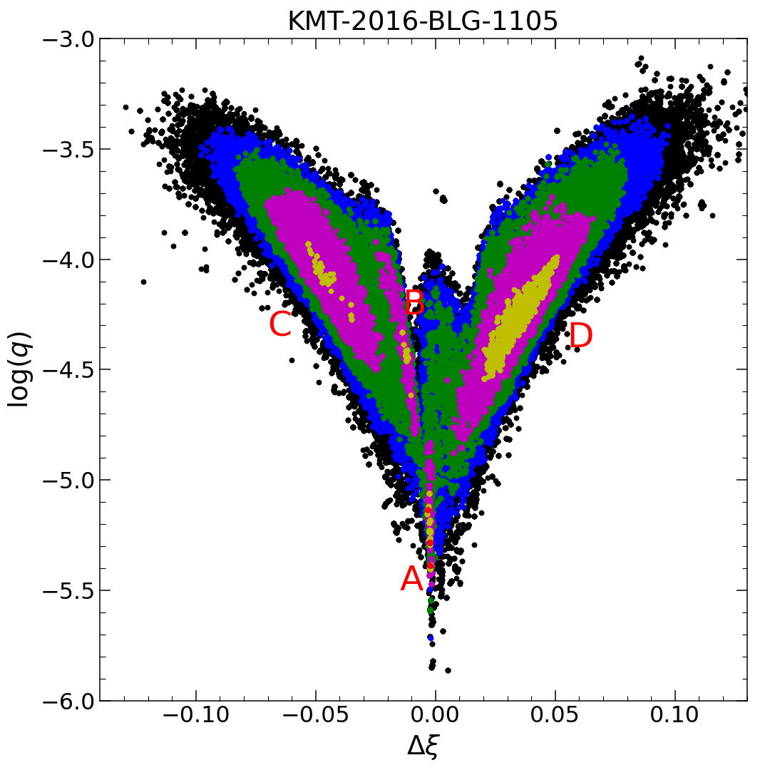
Figure 12: Scatter plot of $\log q$ vs. $\Delta\xi$ for KMT-2016-BLG-1105. The distribution is derived by inflating the error bars by a factor of $\sqrt{2.5}$ and then multiplying the resulting $\chi^{2}$ by 2.5 for the plot. The colors are the same as those in Figure 3. “A”, “B”, “C”, and “D” represent four local minima and the corresponding parameters are given in Table 9.

For the four “Wide” solutions, the “Wide A” and “Wide B” solutions have a source crossing the planetary caustic, and the “Wide C” and “Wide D” solutions that contain a source that passes to one side or the other of the planetary caustic. This topology is qualitatively similar to the topology of OGLE-2017-BLG-0173 (Hwang et al., 2018a). We thus also investigate the parameter space by a “hotter” MCMC with the error bar inflated by a factor of $\sqrt{2.5}$. The resulting scatter plot is shown in Figure 12, from which we find that the topology of KMT-2016-BLG-1105 has differences in three aspects from the topology of OGLE-2017-BLG-0173. First, for the two solutions in which the source passes to one side or the other of the planetary caustic, OGLE-2017-BLG-0173 has caustic crossings and the source is comparable to the size of the planetary caustic, but in the present case, the source does not cross the caustic. Second, for the solution in which the source passes directly over the planetary caustic, the source is much larger than the planetary caustics in the case of OGLE-2017-BLG-0173, while the source of KMT-2016-BLG-1105 is smaller than the caustic. Third, OGLE-2017-BLG-0173 exhibits a bimodal minimum when the source passes directly over the caustic, and the mass-ratio difference between the two local minima is $\Delta\log q<0.1$. The corresponding solutions for KMT-2016-BLG-1105, the “Wide A” and “Wide B” solutions, have $\Delta\log q\sim 1$. We note that the “Wide A” and “Wide B” solutions have $\Delta\xi\sim$ 0.00 and $-$0.01, respectively. Considering the approximate symmetry with respect to $\Delta\xi$, one might expect an additional minimum that has $\Delta\xi\sim 0.01$ and a similar $\log q$ as the $\log q$ of the “Wide B” solution. However, such a potential solution “disappeared” from the numerical analysis. Because the trajectories of the “Wide” B solution and the putative minimum at $\Delta\xi\sim 0.01$ should be almost symmetric with respect to the center of the caustics, their corresponding planetary signals should also be almost symmetric. As shown in Figure 10, the “Wide B” solution drops rapidly during the caustic exit, followed by a dip, so the putative minimum at $\Delta\xi\sim 0.01$ should contain a dip followed by a sudden rise during the caustic entry, which is not supported by the KMTC and KMTS data. Thus, in Figure 12 this topology is absorbed into the MCMC chain of the “Wide D” solution and there is no new discrete solution.

We also check whether the bump-type anomaly can be fitted by a 1L2S model. Table 8 lists the 1L2S parameters. We find that the best-fit 1L2S model is disfavored by $\Delta\chi^{2}=12.0$ compared to the best-fit 2L1S model. The best-fit 1L2S model has $\rho_{2}=0.0018$. We note that the flux ratio is $q_{f,I}\sim 2\times 10^{-3}$, corresponding to a magnitude difference of 6.7 mag. According to Section 5, the primary source lies 4.1 mag below the red giant clump, so the putative source companion would have an absolute magnitude of $M_{I,2}\sim 10.7$ mag, corresponding to an angular source radius of $\theta_{*,2}\sim 0.1~{}\mu$as. This yields the lens-source relative proper motion of $\mu_{\rm rel}=\theta_{*,2}/\rho_{2}/t_{\rm E}\sim 0.5~{}{\rm mas\,yr^{-1}}$, which is lower than the typical $\mu_{\rm rel}$ of bulge microlensing events (See Figure 2 of Zhu et al. (2017) for examples). However, a model with $\rho_{2}=0$ is only disfavored by $\Delta\chi^{2}=1$, so any reasonable $\mu_{\rm rel}$ is only disfavored by $\Delta\chi^{2}<1$. Thus, while the planetary model is strongly favored, there is a possibility that the anomaly is caused by a second source.

With high-order effects, we find that $\Delta\chi^{2}<1$ and the $1\sigma$ uncertainty of parallax is $>0.9$ at all directions, so the constraint on ${\pi}_{\rm E}$ is not useful.

5 Source and Lens Properties

5.1 Preamble

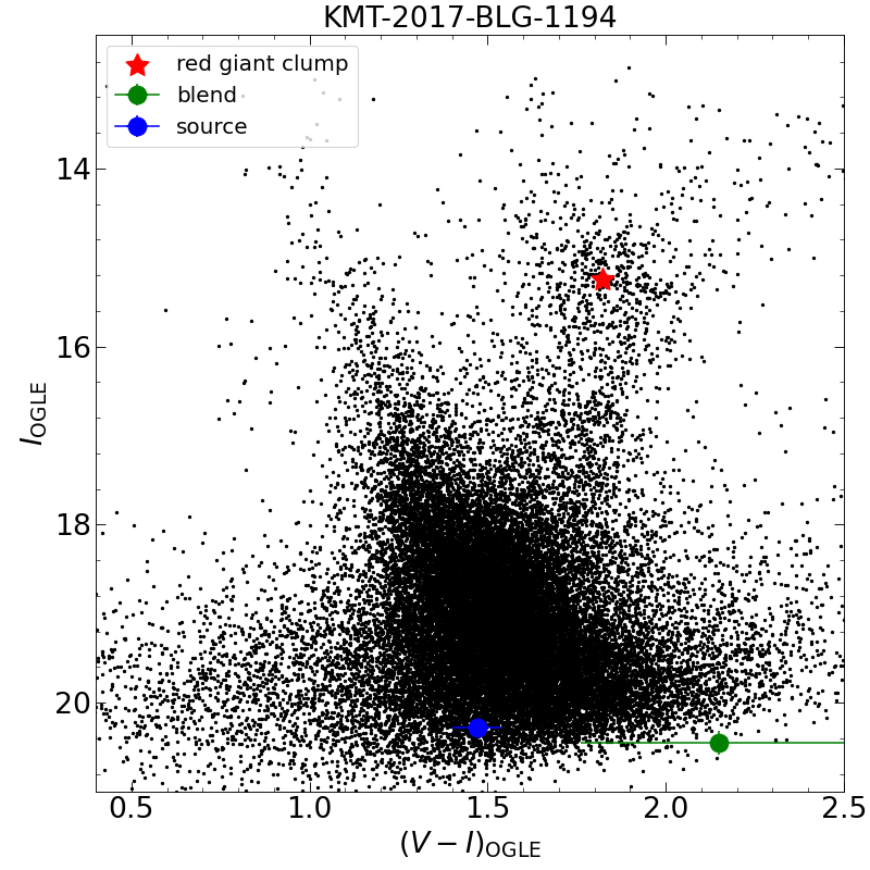
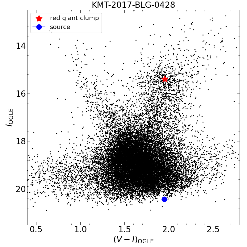
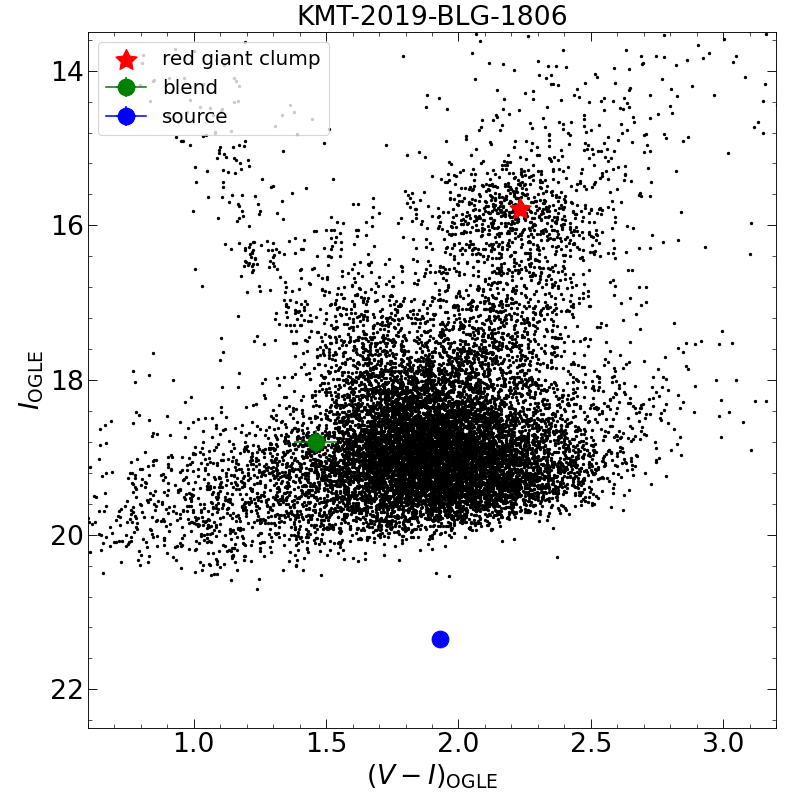
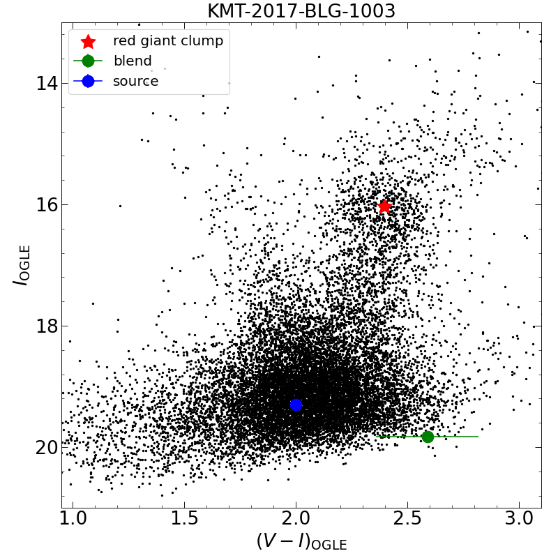
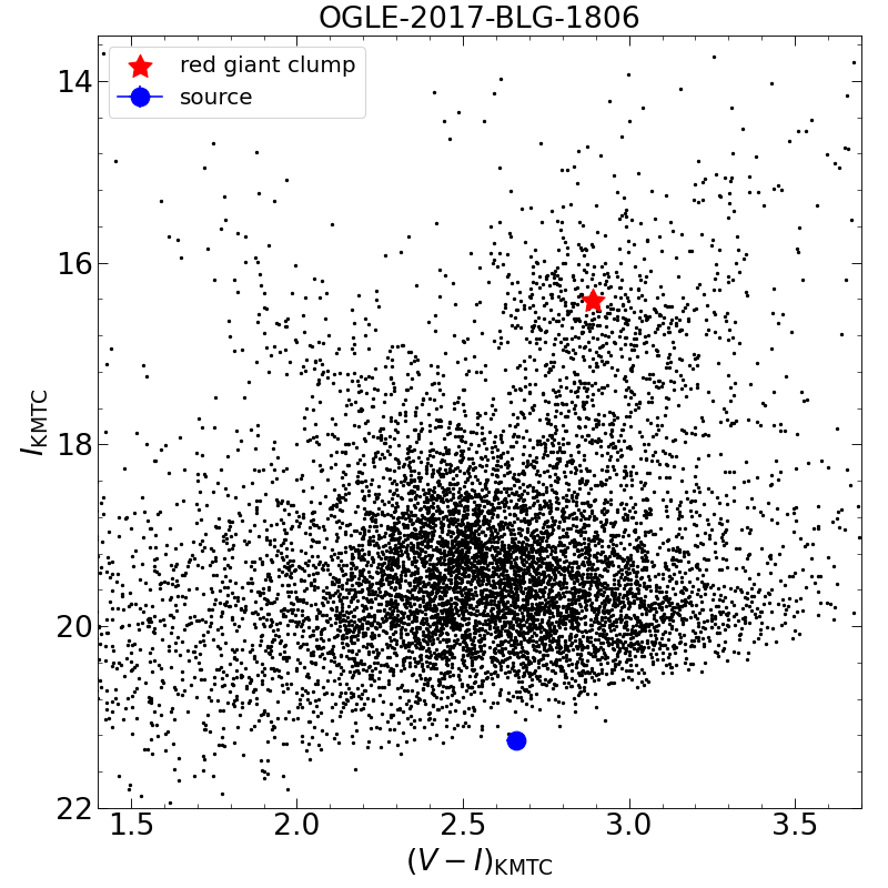
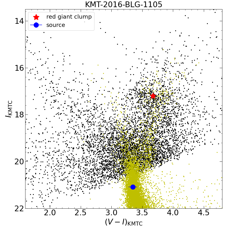
Figure 13: Color magnitude diagrams for the seven planetary events analyzed in this paper. The first five CMDs are constructed using the OGLE-III star catalog (Szymański et al., 2011), and the other two CMDs are constructed using the KMTC pyDIA photometry reduction. For each panel, the red asterisk and the blue dot are shown as the centroid of the red giant clump and the microlensed source star, respectively. The three green dots on the CMDs of KMT-2017-BLG-1194, KMT-2019-BLG-1806, and KMT-2017-BLG-1003 represent the blended light. For the bottom panel, the yellow dots represent the HST CMD of Holtzman et al. (1998) whose red-clump centroid has been matched to that of KMTC using $(V-I,I)_{\rm cl,HST}=(1.62,15.15)$ (Bennett et al., 2008).

Combining Equations (1) and (7), the mass $M_{\rm L}$ and distance $D_{\rm L}$ of a lens system are related to the angular Einstein radius $\theta_{\rm E}$ and the microlensing parallax ${\pi}_{\rm E}$ by (Gould, 1992, 2000)

$$M_{\rm L}=\frac{\theta_{\rm E}}{{\kappa}{\pi}_{\rm E}};\qquad D_{\rm L}=\frac{\mathrm{au}}{{\pi}_{\rm E}\theta_{\rm E}+\pi_{\rm S}},$$ (18)

Table 10: CMD parameters, $\theta_{*}$, $\theta_{\rm E}$ and $\mu_{\rm rel}$ for the five “dip” planetary events

Parameter	KB171194	KB170428	KB191806	KB171003		KB191367
				Inner	Outer
$(V-I)_{\rm cl}$	$1.82\pm 0.01$	$1.95\pm 0.01$	$2.23\pm 0.01$	$2.39\pm 0.01$	$\leftarrow$	$1.70\pm 0.01$
$I_{\rm cl}$	$15.25\pm 0.01$	$15.39\pm 0.01$	$15.79\pm 0.02$	$16.04\pm 0.01$	$\leftarrow$	$15.13\pm 0.01$
$I_{\rm cl,0}$	$14.26\pm 0.04$	$14.36\pm 0.04$	$14.39\pm 0.04$	$14.34\pm 0.04$	$\leftarrow$	$14.37\pm 0.04$
$(V-I)_{\rm S}$	$1.47\pm 0.07$	$1.95\pm 0.04$	$1.93\pm 0.03$	$2.00\pm 0.02$	$\leftarrow$	$1.70\pm 0.03$
$I_{\rm S}$	$20.28\pm 0.08$	$20.43\pm 0.05$	$21.35\pm 0.07$	$19.30\pm 0.04$	$19.30\pm 0.04$	$21.47\pm 0.13$
$(V-I)_{\rm S,0}$	$0.71\pm 0.08$	$1.06\pm 0.05$	$0.76\pm 0.05$	$0.67\pm 0.04$	$\leftarrow$	$1.06\pm 0.04$
$I_{\rm S,0}$	$19.29\pm 0.09$	$19.40\pm 0.07$	$19.95\pm 0.08$	$17.60\pm 0.06$	$17.60\pm 0.06$	$20.71\pm 0.14$
$\theta_{*}$ ($\mu$as)	$0.448\pm 0.038$	$0.578\pm 0.034$	$0.345\pm 0.020$	$0.942\pm 0.046$	$0.942\pm 0.046$	$0.316\pm 0.023$
$\theta_{\rm E}$ (mas)	$>0.17$	$>0.09$	$>0.19$	$>0.14$	$0.180\pm 0.041$	$>0.06$
$\mu_{\rm rel}$ (${\rm mas\,yr^{-1}}$)	$>1.3$	$>0.74$	$>0.51$	$>2.0$	$2.56\pm 0.58$	$>0.53$

Table 11: CMD parameters, $\theta_{*}$, $\theta_{\rm E}$ and $\mu_{\rm rel}$ for OGLE-2017-BLG-1806.

Parameter	Close A		Close B		Wide
	$u_{0}>0$	$u_{0}<0$	$u_{0}>0$	$u_{0}<0$	$u_{0}>0$	$u_{0}<0$
$(V-I)_{\rm cl}$	$2.89\pm 0.01$	$\leftarrow$	$\leftarrow$	$\leftarrow$	$\leftarrow$	$\leftarrow$
$I_{\rm cl}$	$16.42\pm 0.02$	$\leftarrow$	$\leftarrow$	$\leftarrow$	$\leftarrow$	$\leftarrow$
$I_{\rm cl,0}$	$14.33\pm 0.04$	$\leftarrow$	$\leftarrow$	$\leftarrow$	$\leftarrow$	$\leftarrow$
$(V-I)_{\rm S}$	$2.66\pm 0.03$	$\leftarrow$	$\leftarrow$	$\leftarrow$	$\leftarrow$	$\leftarrow$
$I_{\rm S}$	$21.12\pm 0.07$	$21.07\pm 0.07$	$21.10\pm 0.08$	$21.10\pm 0.08$	$21.03\pm 0.07$	$21.08\pm 0.07$
$(V-I)_{\rm S,0}$	$0.83\pm 0.04$	$\leftarrow$	$\leftarrow$	$\leftarrow$	$\leftarrow$	$\leftarrow$
$I_{\rm S,0}$	$19.03\pm 0.08$	$18.98\pm 0.08$	$19.01\pm 0.09$	$19.01\pm 0.09$	$18.94\pm 0.08$	$18.99\pm 0.08$
$\theta_{*}$ ($\mu$as)	$0.561\pm 0.031$	$0.574\pm 0.031$	$0.566\pm 0.033$	$0.566\pm 0.033$	$0.584\pm 0.032$	$0.571\pm 0.032$
$\theta_{\rm E}$ (mas)	$0.322_{-0.145}^{+0.083}$	$0.314_{-0.138}^{+0.087}$	$0.377_{-0.157}^{+0.120}$	$0.343_{-0.141}^{+0.105}$	$>0.21$	$>0.24$
$\mu_{\rm rel}$ (${\rm mas\,yr^{-1}}$)	$1.69^{+0.45}_{-0.77}$	$1.72^{+0.49}_{-0.76}$	$1.98^{+0.64}_{-0.84}$	$2.08^{+0.65}_{-0.87}$	$>1.2$	$>1.3$

Table 12: CMD parameters, $\theta_{*}$, $\theta_{\rm E}$ and $\mu_{\rm rel}$ for KMT-2016-BLG-1105.

	Wide A	Wide B	Wide C	Wide D	Close
$I_{\rm cl}$	$17.20\pm 0.01$	$\leftarrow$	$\leftarrow$	$\leftarrow$	$\leftarrow$
$I_{\rm cl,0}$	$14.39\pm 0.04$	$\leftarrow$	$\leftarrow$	$\leftarrow$	$\leftarrow$
$I_{\rm S}$	$21.09\pm 0.08$	$21.20\pm 0.05$	$21.22\pm 0.11$	$21.22\pm 0.11$	$21.27\pm 0.06$
$(V-I)_{\rm S,0}$	$0.74\pm 0.07$	$0.75\pm 0.07$	$0.75\pm 0.07$	$0.75\pm 0.07$	$0.75\pm 0.07$
$I_{\rm S,0}$	$18.28\pm 0.09$	$18.39\pm 0.07$	$18.41\pm 0.12$	$18.41\pm 0.12$	$18.46\pm 0.07$
$\theta_{*}$ ($\mu$as)	$0.732\pm 0.057$	$0.702\pm 0.051$	$0.696\pm 0.061$	$0.696\pm 0.061$	$0.680\pm 0.050$
$\theta_{\rm E}$ (mas)	$>0.31$	$0.240\pm 0.070$	$>0.15$	$>0.13$	$0.907\pm 0.182$
$\mu_{\rm rel}$ (${\rm mas\,yr^{-1}}$)	$>2.9$	$2.07\pm 0.62$	$>1.3$	$>1.1$	$7.65\pm 1.54$

To obtain the angular Einstein radius through $\theta_{\rm E}=\theta_{*}/\rho$, we first estimate the angular source radius $\theta_{*}$ by locating the source on a color-magnitude diagram (CMD, Yoo et al. 2004). For each event, we construct a $V-I$ versus $I$ CMD using the ambient stars of the OGLE-III catalog (Szymański et al., 2011) or the KMTC images with the pyDIA reductions. See Figure 13 for the CMDs of the seven planetary events. We estimate the centroid of the red giant clump as $(V-I,I)_{\rm cl}$ from CMDs and adopt the de-reddened color and magnitude of the red giant clump, $(V-I,I)_{\rm cl,0}$, from Bensby et al. (2013) and Table 1 of Nataf et al. (2013). We obtain the source apparent magnitude from the light-curve analysis of Section 4, and the source color by a regression of the KMTC $V$ versus $I$ flux with the change of the lensing magnification.

We find that the $V$-band observations of KMT-2016-BLG-1105 have insufficient signal-to-noise ratio to determine the source color, so we estimate the source color by the Hubble Space Telescope (HST) CMD of Holtzman et al. (1998) (see Section 5.7 for details). Finally, using the color/surface-brightness relation of Adams et al. (2018), we obtain the angular source radius $\theta_{*}$. Tables 10, 11 and 12 present the CMD values and ($\theta_{*}$, $\theta_{\rm E}$, $\mu_{\rm rel}$) from the procedures above.

Because the blended light could provide additional constraints on the lens properties (e.g., the upper limits for the lens brightness), we also check the brightness and the astrometric alignment of the baseline object. For KMT-2017-BLG-0428 and KMT-2019-BLG-1806, we adopt the $i^{\prime}$-band baseline images taken by the 3.6m Canada-France-Hawaii Telescope (CFHT) from 2020 to 2022, whose seeing FWHM is $0.^{\prime\prime}55$–$0.^{\prime\prime}70$. For the other five events which do not have any CFHT image, we check the baseline objects from the KMTC pyDIA reduction, whose seeing FWHM is about $1.^{\prime\prime}0$.

Because none of the seven planetary events have simultaneous measurements of ${\pi}_{\rm E}$ and $\theta_{\rm E}$ at the $>3\sigma$ level, the lens masses and distances cannot be directly determined by Equation (18). We conduct a Bayesian analysis using a Galactic model to estimate the lens properties. The Galactic model and the procedures we adopt are the same as described in Zang et al. (2021b). We refer the reader to that work for details. The only exception is that we include upper limits of the lens light, $I_{\rm L,limit}$, from the analysis of the blended light. We adopt the mass-luminosity relation of Wang et al. (2018),

$$M_{I}=4.4-8.5\log{\frac{M_{\rm L}}{M_{\odot}}},$$ (19)

where $M_{I}$ is the absolute magnitude in the $I$ band, and we reject trial events for which the lens properties obey

$$M_{I}+5\log{\frac{D_{\rm L}}{10{\rm pc}}}+A_{I,D_{\rm L}}<I_{\rm L,limit},$$ (20)

where $A_{I,D_{\rm L}}$ is the extinction at $D_{\rm L}$. We adopt an extinction curve with a scale height of 120 pc. For the five events with OGLE CMDs, the total extinction is derived from the CMD analysis, $A_{I}=I_{\rm cl}-I_{\rm cl,0}$. For the other two events with KMTC CMDs, we adopt the extinction in the $K$ band from Gonzalez et al. (2012) and $A_{I}=7.26~{}A_{K}$ from Nataf et al. (2016).

Table 13: Physical parameters of the six planetary events from a Bayesian analysis.

Event	Solution	Physical Properties					Relative Weights
		$M_{\rm host}[M_{\odot}]$	$M_{\rm planet}[M_{\oplus}]$	$D_{\rm L}$[kpc]	$a_{\bot}$[au]	$\mu_{\rm rel}$[${\rm mas\,yr^{-1}}$]	Gal.Mod.	$\chi^{2}$
KB171194		$0.41_{-0.19}^{+0.23}$	$3.54_{-1.63}^{+1.95}$	$4.24_{-1.71}^{+2.16}$	$1.78_{-0.46}^{+0.45}$	$4.29_{-1.66}^{+2.50}$	…	…
KB170428	Inner	$0.34_{-0.17}^{+0.22}$	$5.63_{-2.85}^{+3.59}$	$5.40_{-2.60}^{+1.82}$	$1.78_{-0.58}^{+0.54}$	$3.27_{-1.32}^{+2.26}$	0.99	1.00
	Outer	$0.34_{-0.17}^{+0.22}$	$5.55_{-2.81}^{+3.53}$	$5.40_{-2.60}^{+1.82}$	$1.85_{-0.60}^{+0.55}$	$3.28_{-1.34}^{+2.24}$	1.00	0.95
	Combined	$0.34_{-0.17}^{+0.22}$	$5.59_{-2.83}^{+3.57}$	$5.40_{-2.60}^{+1.82}$	$1.81_{-0.59}^{+0.55}$	$3.27_{-1.32}^{+2.26}$	…	…
KB191806	Inner ($u_{0}>0$)	$0.75_{-0.25}^{+0.24}$	$4.67_{-1.52}^{+1.52}$	$6.62_{-1.93}^{+0.72}$	$2.87_{-0.66}^{+0.64}$	$1.17_{-0.34}^{+0.70}$	1.00	0.70
	Inner ($u_{0}<0$)	$0.74_{-0.26}^{+0.25}$	$4.47_{-1.52}^{+1.56}$	$6.63_{-2.01}^{+0.73}$	$2.85_{-0.70}^{+0.66}$	$1.11_{-0.34}^{+0.74}$	0.84	0.58
	Outer ($u_{0}>0$)	$0.73_{-0.26}^{+0.25}$	$4.63_{-1.64}^{+1.60}$	$6.68_{-1.97}^{+0.72}$	$3.11_{-0.79}^{+0.73}$	$1.13_{-0.36}^{+0.70}$	0.98	0.82
	Outer ($u_{0}<0$)	$0.75_{-0.25}^{+0.24}$	$4.79_{-1.60}^{+1.56}$	$6.62_{-2.09}^{+0.74}$	$3.17_{-0.75}^{+0.70}$	$1.15_{-0.36}^{+0.74}$	0.98	1.00
	Combined	$0.74_{-0.25}^{+0.25}$	$4.67_{-1.60}^{+1.56}$	$6.64_{-2.01}^{+0.72}$	$3.02_{-0.73}^{+0.70}$	$1.13_{-0.34}^{+0.74}$	…	…
KB171003	Inner	$0.37_{-0.19}^{+0.32}$	$6.75_{-3.44}^{+5.79}$	$7.03_{-0.74}^{+0.61}$	$1.54_{-0.37}^{+0.38}$	$3.55_{-0.84}^{+0.88}$	1.00	0.90
	Outer	$0.27_{-0.13}^{+0.26}$	$3.72_{-1.80}^{+3.71}$	$7.16_{-0.65}^{+0.61}$	$1.25_{-0.25}^{+0.27}$	$2.75_{-0.54}^{+0.56}$	0.74	1.00
	Combined	$0.32_{-0.17}^{+0.31}$	$5.19_{-2.80}^{+5.39}$	$7.09_{-0.70}^{+0.61}$	$1.38_{-0.32}^{+0.39}$	$3.11_{-0.72}^{+0.94}$	…	…
KB191367	Inner	$0.25_{-0.13}^{+0.16}$	$4.06_{-2.08}^{+2.56}$	$4.68_{-2.10}^{+2.44}$	$1.67_{-0.55}^{+0.49}$	$3.92_{-1.71}^{+2.57}$	1.00	1.00
	Outer	$0.25_{-0.13}^{+0.16}$	$4.12_{-2.10}^{+2.58}$	$4.67_{-2.10}^{+2.45}$	$1.73_{-0.57}^{+0.51}$	$3.89_{-1.71}^{+2.55}$	0.96	0.90
	Combined	$0.25_{-0.13}^{+0.16}$	$4.08_{-2.08}^{+2.58}$	$4.67_{-2.10}^{+2.45}$	$1.70_{-0.56}^{+0.50}$	$3.91_{-1.71}^{+2.56}$	…	…
OB171806	Close A ($u_{0}>0$)	$0.44_{-0.23}^{+0.33}$	$5.87_{-3.04}^{+4.43}$	$6.60_{-1.06}^{+0.65}$	$1.84_{-0.51}^{+0.44}$	$1.95_{-0.54}^{+0.46}$	0.85	0.90
	Close A ($u_{0}<0$)	$0.33_{-0.16}^{+0.33}$	$4.83_{-2.44}^{+4.83}$	$6.17_{-1.57}^{+0.92}$	$1.69_{-0.43}^{+0.46}$	$2.13_{-0.58}^{+0.56}$	1.00	1.00
	Close B ($u_{0}>0$)	$0.44_{-0.26}^{+0.39}$	$2.40_{-1.48}^{+2.24}$	$5.95_{-2.13}^{+1.11}$	$1.89_{-0.62}^{+0.58}$	$2.39_{-0.70}^{+0.78}$	0.21	$10^{-3.1}$
	Close B ($u_{0}<0$)	$0.48_{-0.26}^{+0.35}$	$2.68_{-1.48}^{+1.96}$	$6.53_{-1.41}^{+0.69}$	$1.91_{-0.58}^{+0.50}$	$2.09_{-0.60}^{+0.58}$	0.16	$10^{-3.2}$
	Wide ($u_{0}>0$)	$0.34_{-0.16}^{+0.31}$	$5.47_{-2.60}^{+4.87}$	$3.01_{-1.09}^{+2.22}$	$2.53_{-0.78}^{+1.06}$	$4.92_{-1.94}^{+1.74}$	$10^{-1.5}$	$10^{-1.8}$
	Wide ($u_{0}<0$)	$0.41_{-0.17}^{+0.23}$	$4.87_{-2.00}^{+2.72}$	$2.87_{-0.86}^{+1.13}$	$2.82_{-0.78}^{+0.85}$	$5.48_{-1.42}^{+1.30}$	0.24	$10^{-1.8}$
	Combined	$0.38_{-0.20}^{+0.34}$	$5.27_{-2.72}^{+4.71}$	$6.40_{-1.51}^{+0.77}$	$1.75_{-0.47}^{+0.46}$	$2.05_{-0.56}^{+0.52}$	…	…
KB161105	Wide A	$0.43_{-0.20}^{+0.22}$	$0.92_{-0.44}^{+0.44}$	$3.79_{-1.44}^{+1.38}$	$2.93_{-0.91}^{+0.69}$	$6.48_{-1.30}^{+2.08}$	0.37	1.00
	Wide B	$0.37_{-0.21}^{+0.31}$	$4.67_{-2.64}^{+3.75}$	$7.12_{-1.10}^{+0.65}$	$2.03_{-0.53}^{+0.52}$	$2.29_{-0.56}^{+0.62}$	1.00	0.32
	Wide C	$0.43_{-0.23}^{+0.27}$	$12.14_{-6.31}^{+7.63}$	$5.42_{-2.33}^{+1.85}$	$2.63_{-0.83}^{+0.79}$	$3.97_{-1.58}^{+2.68}$	0.66	0.11
	Wide D	$0.44_{-0.23}^{+0.27}$	$9.51_{-4.87}^{+5.75}$	$5.28_{-2.23}^{+1.92}$	$2.56_{-0.74}^{+0.73}$	$4.11_{-1.56}^{+2.64}$	0.64	0.26
	Close	$0.43_{-0.18}^{+0.18}$	$1.32_{-0.56}^{+0.56}$	$3.27_{-1.15}^{+1.28}$	$2.26_{-0.69}^{+0.51}$	$6.74_{-1.58}^{+1.74}$	0.29	0.17
	Combined	$0.41_{-0.21}^{+0.25}$	$2.32_{-1.56}^{+7.43}$	$5.08_{-2.18}^{+2.24}$	$2.44_{-0.75}^{+0.88}$	$4.68_{-2.50}^{+2.76}$	…	…

Table 13 presents the resulting Bayesian estimates of the host mass $M_{\rm host}$, the planet mass $M_{\rm planet}$, the lens distance $D_{\rm L}$, the projected planet-host separation $a_{\bot}$ and the lens-source relative proper motion $\mu_{\rm rel}$. For events with multiple solutions, we show the results for each solution and the “combined results” of combining all solutions weighted by their Galactic-model likelihood and ${\rm exp}(-\Delta\chi^{2}/2)$, where $\Delta\chi^{2}$ is the $\chi^{2}$ difference compared to the best-fit solution. Here the Galactic-model likelihood represents the total weight for the simulated events given the error distributions of $t_{\rm E},\theta_{\rm E}$ and ${\pi}_{\rm E}$. See Equation (16) of Zang et al. (2021b) for the weight procedures.

We do not adopt the “combined results” as the final physical parameters but just show them for consideration, because there is no conclusion about how to combine degenerate solutions. We note that the ${\rm exp}(-\Delta\chi^{2}/2)$ probability might be suffered from systematic errors of the observed data. However, the weight from $\Delta\chi^{2}$ only has minor effects on the “combined results”. Except for KMT-2016-BLG-1105 the degenerate solutions have similar physical interpretations and except for OGLE-2017-BLG-1806 the $\Delta\chi^{2}$ is small, but for OGLE-2017-BLG-1806 the “combined results” are already dominated by the “Close A” solutions due to their Galactic-model likelihoods. Due to similar reasons, whether to include the phase-space factors also has a minor impact on the “combined results”.

5.2 KMT-2017-BLG-1194

The corresponding CMD shown in Figure 13 is constructed from the OGLE-III field stars within $240^{\prime\prime}$ centered on the event. The baseline object has $(V,I)_{\rm base}=(21.343\pm 0.085,19.608\pm 0.051)$, yielding a blend of $(V-I,I)_{\rm B}=(2.15\pm 0.39,20.45\pm 0.14)$. We display the blend on the CMD. The source position measured by the difference imaging analysis is displaced from the baseline object by $\Delta\theta(N,E)=(-26,41)$ mas. We estimate the error of the baseline position by the fractional astrometric error being equal to the fractional photometric error (Jung et al., 2020), which yields $\sigma_{\rm ast}=0.39\sigma_{I}{\rm FWHM}=20$ mas. We note that the astrometric error should be underestimated due to the mottled background from unresolved stars and other systematic errors, but the whole astrometric error should be not more than twice our estimate. Thus, the baseline object is astrometrically consistent with the source and the lens within $2\sigma$. The blend does not have a useful color constraint. We adopt the $3\sigma$ upper limit of the blended light, $I_{\rm L,limit}=20.03$, as the upper limit of the lens brightness.

As given in Table 13, the preferred host star is an M dwarf located in the Galactic disk, and the planet is probably a super-Earth beyond the snow line of the lens system (assuming a snow line radius $a_{\rm SL}=2.7(M/M_{\odot})$ au, Kennedy & Kenyon 2008).

5.3 KMT-2017-BLG-0428

The corresponding CMD shown in Figure 13 consists of the OGLE-III field stars within $150^{\prime\prime}$ centered on the event. The baseline object on the CFHT images has $I_{\rm base}=20.056\pm 0.063$, with an astrometric offset of $\Delta\theta(N,E)=(6,-2)$ mas and an astrometric error of $\sigma_{\rm ast}\sim 5$ mas. Thus, the baseline object is astrometrically consistent with the source at about $1\sigma$. Because the CFHT images do not contain color information, we do not display the blend on the CMD. We also adopt the $3\sigma$ upper limit of the blended light, $I_{\rm L,limit}=20.81$, as the upper limit of the lens brightness.

As shown in Table 13, the Bayesian analysis indicates another cold super-Earth orbiting an M dwarf.

5.4 KMT-2019-BLG-1806

The CMD of this event is constructed from the OGLE-III field stars within $150^{\prime\prime}$ centered on the event, shown in Figure 13. The baseline object on the KMTC images has $(V,I)_{\rm base}=(20.155\pm 0.125,18.685\pm 0.076)$. We plot the blend on the CMD and find that the blend probably belongs to the foreground main-sequence branch and thus could be the lens. However, the astrometric offset is $\Delta\theta(N,E)=(433,-76)$ mas and $\Delta\theta(N,E)=(416,-96)$ mas on the CFHT and KMTC images, respectively, so the majority of the blended light is unrelated to the lens. We adopt the median value of the blended light, $I_{\rm L,limit}=18.8$, as the upper limit of the lens brightness.

The results of the Bayesian analysis are given in Table 13. The planet is another cold super-Earth, and the preferred host is a K dwarf.

5.5 KMT-2017-BLG-1003

We use the OGLE-III field stars within $180^{\prime\prime}$ centered on the event to build the CMD. Combining the measured $\rho$ from the light-curve analysis, we obtain $\theta_{\rm E}=0.180\pm 0.041$ mas for the “Outer” solution and $\theta_{\rm E}>0.14$ mas ($3\sigma$) for the “Inner” solution. The KMTNet baseline object has $(V,I)_{\rm base}=(20.968\pm 0.046,18.780\pm 0.028)$, corresponding to a blend of $(V-I,I)_{\rm B}=(2.54\pm 0.20,19.83\pm 0.10)$, and we display the blend on the CMD. The source-baseline astrometric offset is $\Delta\theta(N,E)=(-64,-77)$ mas, with an astrometric error of $\sigma_{\rm ast}\sim 12$ mas, implying that most of the blend light should be unrelated to the event. We adopt the median value of the blended light, $I_{\rm L,limit}=19.83$, as the upper limit of the lens brightness.

The Bayesian analysis shows that the host star is probably an M dwarf located in the Galactic bulge. Again, the preferred planet is a cold super-Earth.

5.6 KMT-2019-BLG-1367

In Figure 13, we display the position of the source on the CMD of stars within $180^{\prime\prime}$ around the source. On the KMTC images, there is no star within $1.^{\prime\prime}4$ around the source position. We thus adopt the detection limit of the KMTC images, $I=21.0$, as the upper limit of the baseline brightness, yielding the $3\sigma$ upper limit of the blended light, $I_{\rm L,limit}=21.6$. Applying Equations (19) and (20) and assuming $D_{\rm L}<8$ kpc, this flux constraint corresponds to an upper limit of the lens mass of $0.6M_{\odot}$.

As shown in Table 13, the Bayesian estimate shows another cold super-Earth orbiting an M dwarf.

5.7 OGLE-2017-BLG-1806

The CMD of this event is constructed from KMTC field stars within a $300^{\prime\prime}$ square centered on the event position. The baseline object, $(V,I)_{\rm base}=(22.300\pm 0.308,20.042\pm 0.128)$, is displaced from the source by 835 mas. Thus, most of the blend light should be unrelated to the event. We do not show the blend on the CMD and adopt the median value of the blended light, $I_{\rm L,limit}=20.5$, as the upper limit of the lens brightness.

The results of the Bayesian analysis are presented in Table 13, and all solutions indicate a cold super-Earth orbiting a low-mass star. The constraints on $\pi_{\rm E,\bot}$ from the light-curve analysis are useful. The “Wide” solution has a relatively large $\theta_{\rm E}$, with a $2\sigma$ lower limit of $0.60$ mas and the best-fit value of $\sim 1.1$ mas, so the corresponding lens system is located in the Galactic disk. Then, the “Wide ($u_{0}>0$)” solution has $\pi_{\rm E,\bot}<0$ and thus a lens velocity in Galactic coordinates of $v_{\ell}\sim 100$ km s^-1, so this solution is strongly disfavored. For the two “Close” solutions, both the $\pi_{\rm E,\bot}<0$ solutions are slightly disfavored and have relatively higher probabilities of a bulge lens system.

For the “Wide” solution, the predicted apparent magnitude of the lens system is fainter than the source by $\sim 0.8$ mag in the $H$ band. In the case of OGLE-2012-BLG-0950, the source and the lens have roughly equal brightness and were resolved by the Keck AO imaging and the HST imaging when they were separated by about 34 mas (Bhattacharya et al., 2018). For OGLE-2017-BLG-1806, we estimate that resolving the lens and source probably requires a separation of 45 mas for the “Wide” solution. We note that the proper motions of the two “Close” solutions are $\sim 2~{}{\rm mas\,yr^{-1}}$. If high-resolution observations resolve the lens and the source and find that $\mu_{\rm rel}$ (e.g., $\sim 5~{}{\rm mas\,yr^{-1}}$) is much higher than that of the “Close” solutions, the three solutions can be distinguished. Such observations can be taken in 2026 or earlier.

5.8 KMT-2016-BLG-1105

To collect enough red-giant stars to determine the centroid of the red giant clump, the CMD of this event shown in Figure 13 contains KMTC field stars within a $280^{\prime\prime}\times 300^{\prime\prime}$ rectangle region. Because the event lies about $80^{\prime\prime}$ from the edge of the CCD chip, it is displaced from the center of the rectangle region by about $70^{\prime\prime}$. The $V$-band data have insufficient signal-to-noise ratio to determine the source color, so we adopt the method of Bennett et al. (2008) to estimate the source color. We first calibrate the CMD of Holtzman et al. (1998) HST observations to the KMTC CMD using the centroids of red giant clumps. We then estimate the source color by taking the color of the HST field stars whose brightness are within the $5\sigma$ of the source star.

The baseline object has $I_{\rm base}=20.729\pm 0.125$ without color information, so we do not plot the blend on the CMD. The source-baseline astrometric offset is $\Delta\theta(N,E)=(73,166)$ mas, at about $3\sigma$. Because the baseline object is marginally detected on the KMTC images, we adopt the median value of the blended light, $I_{\rm L,limit}=21.7$, as the upper limit of the lens brightness.

The Bayesian analysis indicates that the host star is probably an M dwarf. Due to a factor of $\sim 13$ differences within the mass ratios of the five degenerate solutions, there is a wide range for the planetary mass, from sub-Earth-mass to sub-Neptune-mass. Because no solution has a very different proper motion from other solutions, future high-resolution observations cannot break the degeneracy. However, such observations are still important because the measurements of the host brightness can yield the host mass and distance, which could be used for studying the relation between the planetary occurrence rate and the host properties. For the “Wide A” and “Close” solutions, the predicted apparent magnitude of the lens system is fainter than the source by $\sim 2$ mag and $\sim 3$ mag in the $H$ and $I$ bands, respectively. In 2025, the lens and the source will be separated by $\gtrsim 50$ mas and may be resolved.

6 Discussion

In this paper, we have presented the analysis of seven $q<10^{-4}$ planets. Together with 17 already published and three that will be published elsewhere, the KMTNet AnomalyFinder algorithm has found 27 events that can be fit by $q<10^{-4}$ models from 2016–2019 KMTNet data. For the analysis above and in other published papers, all of the local minima are investigated, but here for each planet, we only consider the models with $\Delta\chi^{2}<10$ compared to the best-fit model.

Table LABEL:tab:-4planet presents the event name, $\log q$, $s$, $u_{0}$, discovery method, $\Delta\chi^{2}$ compared to the best-fit models, whether it has a caustic crossing, anomaly type (bump or dip), and the KMTNet fields (prime or sub-prime) of each planet, ranked-ordered by $\log q$ of the best-fit models. Of them, 15 were solely detected using AnomalyFinder, and 12 were first discovered from by-eye searches and then recovered by AnomalyFinder, which illustrates the importance of systematic planetary anomaly searches in finding low mass-ratio microlensing planets. The seasonal distribution, (5, 8, 8, 6) for 2016–2019, is consistent with normal Poisson variations.

Among the 27 planets, four have alternative possible models with $q>10^{-4}$, and 23 are secure $q<10^{-4}$ planets. Because the detection of $q<10^{-4}$ planets is one of the major scientific goals of the ongoing KMTNet survey and future space-based microlensing projects (Penny et al., 2019; Ge et al., 2022; Yan & Zhu, 2022), it is worthwhile to review the properties of the 27 planetary events and study how to detect more such planets.

6.1 The Missing Planetary Caustics Problem

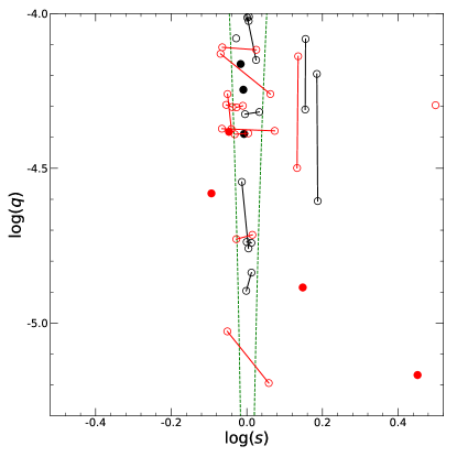
Figure 14: $\log q$ vs. $\log s$ distribution for the 27 planetary events with $q<10^{-4}$ shown in Table LABEL:tab:-4planet, adapted from Figure 11 of Yee et al. (2021). The red points represent planets that were solely detected by AnomalyFinder, and the black points represent planets that were first discovered from by-eye searches and then recovered by AnomalyFinder. Solutions are considered to be “unique” (filled points) if there are no competing solutions within $\Delta\chi^{2}<10$. Otherwise, they are shown by open circles. The event KMT-2016-BLG-1105 has five degenerate solutions, but we only plot the best-fit $s>1$ and $s<1$ solutions for simplicity. For two solutions that are subject to the $u_{0}>0$ and $u_{0}<0$ degeneracy, we show them as one solution and take the average values. The two green dashed lines indicate the boundaries for “near-resonant” caustics (Dominik, 1999).

As illustrated by Zang et al. (2021b), the motivation for building the KMTNet AnomalyFinder algorithm is to exhume the buried signatures of “missing planetary caustics” in the KMTNet data. Zhu et al. (2014) predicted that $\sim 50\%$ of the KMTNet $q<10^{-4}$ planets should be detected by caustics outside of the near-resonant (Dominik, 1999; Yee et al., 2021) range. Below we follow the definitions of Zang et al. (2021b) and refer to caustics inside and outside of the near-resonant range as near-resonant caustics and pure-planetary caustics. Contrary to the prediction of Zhu et al. (2014), before the application of AnomalyFinder only two of ten $q<10^{-4}$ KMTNet planets were detected by pure-planetary caustics. The two cases are OGLE-2017-BLG-0173Lb (Hwang et al., 2018a) and KMT-2016-BLG-0212Lb (Hwang et al., 2018b). Hence, it is necessary to check the caustic types for the planetary sample of AnomalyFinder.

Figure 14 shows the $\log q$ versus $\log s$ plot for the 27 planets. The red and black points represent planets that were first discovered using AnomalyFinder and by-eye searches, respectively. The two green dashed lines indicate the boundaries for the near-resonant range. A striking feature is that in constrast to the locations of the by-eye planets, of the 15 AnomalyFinder planets 11 have pure-planetary caustics, two have both pure-planetary and near-resonant caustics, and only two are fully located inside the near-resonant range. In total, at least 13 planets were detected by pure-planetary caustics. Thus, the caustic types of the AnomalyFinder planetary sample agree with the expectation of Zhu et al. (2014), and the missing planetary caustics problem has been solved by the systematic planetary anomaly search.

6.2 Caustic Crossing and Anomaly Type

Zhu et al. (2014) predicted that about half of the KMTNet planets will be detected by caustic-crossing anomalies. Jung et al. (2022) found that 16/33 of 2018 KMTNet AnomalyFinder planets have caustic-crossing anomalies. As shown in Table LABEL:tab:-4planet, 14/27 of the $q<10^{-4}$ planets have caustic-crossing anomalies, in good agreement with the expectation of Zhu et al. (2014). Thus, the $\sim 50\%$ probability of caustic-crossing anomalies is likely applicable down to $q\sim 10^{-5}$.

Zang et al. (2021b) and Hwang et al. (2022) applied the AnomalyFinder algorithm to 2018–2019 KMTNet prime-field events and found seven newly discovered $q<2\times 10^{-4}$ planets. Among them, only OGLE-2019-BLG-1053Lb has a bump-type anomaly and the other six planets were detected by dip-type anomalies. Thus, it is necessary to check whether dip-type anomalies dominate the detection of low-$q$ planets. As presented in Table LABEL:tab:-4planet, the ratio of bump-type to dip-type anomalies for the $q<10^{-4}$ planets is 15 to 12, so the two types of anomalies play roughly equal roles in the low-$q$ detection. However, of the 12 dip-type anomalies, nine were solely detected by AnomalyFinder, including eight non-caustic-crossing anomalies. KMT-2018-BLG-1988 (Han et al., 2022a) is the only case that the anomaly is a non-caustic-crossing dip and was first discovered from by-eye searches. Unlike the dip-type anomalies, the four non-caustic-crossing bumps were all first noticed from by-eye searches. Hence, by-eye searches have proved to be quite insensitive to non-caustic-crossing dip-type anomalies for low-$q$ planets.

6.3 A Desert of High-magnification Planetary Signals

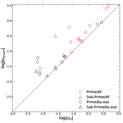
Figure 15: $\log|u_{\rm anom}|$ vs. $\log|u_{0}|$ distribution for the 27 planetary events with $q<10^{-4}$ shown in Table LABEL:tab:-4planet. Colors are the same as the colors of Figure 14. Circles and triangles represent prime-field and sub-prime-field planets, respectively. The grey dashed line indicates $|u_{0}|=|u_{\rm anom}|$.

Zang et al. (2021b) suggested that the missing planetary caustics problem was caused by the way that modelers searched for planetary signatures. Because high-magnification events are intrinsically more sensitive to planets (Griest & Safizadeh, 1998), by-eye searches paid more attention to them, while pure-planetary caustics are mainly detected in low-magnification events. If this hypothesis is correct, we expect that by-eye planets and AnomalyFinder planets will have different $|u_{0}|$ and $|u_{\rm anom}|$ distributions. The $\log|u_{\rm anom}|$ versus $\log|u_{0}|$ distribution of Figure 15 confirms our expectation. Except for the two planets that were detected by pure-planetary caustics, all the other by-eye planets, which are located inside the near-resonant range, were detected with $|u_{0}|\lesssim 0.05$ and $|u_{\rm anom}|\lesssim 0.07$. The roughly one-dex gap of the by-eye planets, at $0.05\lesssim|u_{0}|\lesssim 0.62$ and $0.07\lesssim|u_{\rm anom}|\lesssim 0.78$, is filled by the AnomalyFinder planets.

However, there is no planet located at the left lower corner of Figure 15, with $|u_{0,{\rm limit}}|=0.0060$ and $|u_{\rm anom,limit}|=0.0158$. Although six of the planets were detected in high-magnification events ($|u_{0}|<0.01$), all the planetary signals occurred on the low- and median-magnification regions. This desert of high-magnification planetary signals could be caused by the insufficient observing cadences of the current KMTNet survey. High-magnification planetary signals for $q<10^{-4}$ events are weak and thus require dense observations over the peak. There are three known $q<10^{-4}$ events whose planetary signals occurred on the high-magnification regions ($|u_{\rm anom}|<0.01$). They are OGLE-2005-BLG-169 with $u_{\rm anom}=0.0012$ (Gould et al., 2006), KMT-2021-BLG-0171 with $|u_{\rm anom}|=0.0066$ (Yang et al., 2022), and KMT-2022-BLG-0440 with $|u_{\rm anom}|=0.0041$ (Zhang et al. in prep). The follow-up data played decisive roles in these detections and the combined cadences of survey and follow-up data are higher than $30~{}{\rm hr}^{-1}$, while the highest cadence of the current KMTNet survey is $8~{}{\rm hr}^{-1}$ for about 0.4 deg² from the overlap of two $\Gamma=4~{}{\rm hr}^{-1}$ fields.

However, we note that AnomalyFinder used the KMTNet end-of-year pipeline light curves, for which the photometric quality is not as good as that of TLC re-reductions. For the three follow-up planets, the planetary signals only have $\Delta I<0.05$ mag. Thus, TLC re-reductions may be needed to recover such weak signals in the KMTNet data, and we cannot rule out the possibility that the desert may also be due to the imperfect KMTNet photometric quality. Each year there are about 20 events with $|u_{0}|<0.01$ observed by KMTNet with $\Gamma\geq 4~{}{\rm hr}^{-1}$. The current KMTNet quasi-automated TLC re-reductions pipeline takes $<$1 hr of human effort for each event (H. Yang et al. in prep), so an optimized systematic search for $q<10^{-4}$ planets in the KMTNet high-magnification events can be done very quickly. This search could have important implications for future space-based microlensing projects, because their tentative cadences are similar to or lower than $\Gamma=4~{}{\rm hr}^{-1}$ (Penny et al., 2019; Ge et al., 2022; Yan & Zhu, 2022). If this search demonstrates that high-magnification events need denser observations to capture the weak planetary signals for low-$q$ planets, one could consider conducting (if feasible) ground-based follow-up projects for high-magnification events that are discovered by space-based telescopes. We also note that for the 2018 AnomalyFinder planets (Gould et al., 2022; Jung et al., 2022) and 2019 prime-field AnomalyFinder planets (Zang et al., 2022a), which are complete now, only one $q>10^{-4}$ planet, KMT-2019-BLG-1953Lb, has $|u_{\rm anom}|<|u_{\rm anom,limit}|$. Future analysis of all the 2016–2019 KMTNet should check whether the desert is obvious for more massive planets.

6.4 Prime and sub-Prime Fields

In its 2015 commissioning season, KMTNet observed four fields at a cadence of $\Gamma=6~{}{\rm hr}^{-1}$. To support the 2016–2019 Spitzer microlensing campaign (Gould et al., 2013, 2014a, 2015a, 2015b, 2016, 2018) and find more planets, KMTNet monitored a wider area, with a total of (3, 7, 11, 3) fields at cadences of $\Gamma\sim(4,1,0.4,0.2)~{}{\rm hr}^{-1}$. The three fields with the highest cadence are the KMTNet prime fields and the other 21 are the KMTNet sub-prime fields. See Figure 12 of Kim et al. (2018a) for the field placement. As shown in Table LABEL:tab:-4planet and Figure 15, the prime fields played the main role in the detection of $q<10^{-4}$ planets, as predicted by Henderson et al. (2014), and 17 of 27 planets were detected therein. However, the sub-prime fields are also important and six of the ten lowest-$q$ planets were discovered therein.

For the six planets with $|u_{0}|<0.01$, there is a clear bias in cadences, and only one of them was detected from the sub-prime fields. For the prime and sub-prime fields, the current detection rates are 1.25 and 0.25 per year, respectively. Because $\sim 60\%$ of the KMTNet microlensing events are located in the sub-prime fields, if the sub-prime-field events with $|u_{0}|<0.01$ can had the same cadence as the prime-field events from follow-up observations, each year there would be $(1.25\times(60\%/40\%)-0.25)=1.6$ more $q<10^{-4}$ planets. Because follow-up observations can have higher cadences and capture the high-magnification planetary signals (e.g., Yang et al. 2022), the yield of a follow-up project can be at least two $q<10^{-4}$ planets per year. The reward is not only enlarging the low-$q$ planetary sample, but also an independent check of the statistical results from AnomalyFinder if the follow-up planets can form a homogeneous statistical sample (Gould et al., 2010). However, this reward requires that the KMTNet alert-finder system should alert new events before they reach the high-magnification regions (e.g., $A>20$).

Table 14: Information of 2016–2019 KMTNet AnomalyFinder planetary sample with $q<10^{-4}$ solutions

Event Name	KMTNet Name	$\log q$	$s$	$|u_{0}|$	Method	$\Delta\chi^{2}$	Caustic-Crossing	Anomaly Type	Field
KB1611051	KB161105	$-5.194\pm 0.248$	$1.143\pm 0.009$	0.171	Discovery	0.0	yes	bump	sub-prime
		$-4.423\pm 0.197$	$1.136\pm 0.011$	0.153		2.3	yes
		$-4.184\pm 0.206$	$1.106\pm 0.013$	0.154		2.7	no
		$-5.027\pm 0.080$	$0.888\pm 0.007$	0.148		3.5	no
		$-4.069\pm 0.182$	$0.892\pm 0.005$	0.154		4.4	yes
OB1600072	KB161991	$-5.168\pm 0.131$	$2.829\pm 0.009$	1.253	Discovery		yes	bump	prime
OB1910533	KB191504	$-4.885\pm 0.035$	$1.406\pm 0.011$	0.373	Discovery		yes	bump	prime
OB1909604	KB191591	$-4.830\pm 0.041$	$1.029\pm 0.001$	0.0061	Recovery	0.0	yes	bump	sub-prime
		$-4.896\pm 0.024$	$0.997\pm 0.001$	0.0060		1.0	yes
		$-4.896\pm 0.024$	$0.996\pm 0.001$	0.0059		1.9	yes
		$-4.845\pm 0.043$	$1.028\pm 0.001$	0.0061		2.1	yes
KB1800295	KB180029	$-4.737\pm 0.047$	$0.999\pm 0.002$	0.027	Recovery	0.0	yes	bump	sub-prime
		$-4.746\pm 0.050$	$1.028\pm 0.002$	0.027		0.2	yes
		$-4.740\pm 0.045$	$0.999\pm 0.002$	0.027		2.1	yes
		$-4.736\pm 0.050$	$1.028\pm 0.002$	0.027		2.2	yes
KB1918061	KB191806	$-4.714\pm 0.116$	$1.035\pm 0.009$	0.0255	Discovery	0.0	no	dip	sub-prime
		$-4.717\pm 0.117$	$1.034\pm 0.009$	0.0257		0.4	no
		$-4.724\pm 0.117$	$0.938\pm 0.007$	0.0260		0.7	no
		$-4.734\pm 0.109$	$0.938\pm 0.007$	0.0251		1.1	no
OB1701736	KB171707	$-4.606\pm 0.042$	$1.540\pm 0.031$	0.867	Recovery	0.0	yes	bump	prime
		$-4.195\pm 0.068$	$1.532\pm 0.025$	0.844		3.5	yes
KB1711941	KB171194	$-4.582\pm 0.058$	$0.806\pm 0.010$	0.256	Discovery		no	dip	sub-prime
KB1819887	KB181988	$-4.544_{-0.168}^{+0.300}$	$0.97\pm 0.03$	0.014	Recovery	0.0	no	dip	sub-prime
		$-4.759_{-0.618}^{+0.698}$	$1.01\pm 0.05$	0.014		0.1	no
KB1908428	KB190842	$-4.389\pm 0.031$	$0.983\pm 0.013$	0.0066	Recovery		no	bump	prime
KB1902539	KB190253	$-4.387\pm 0.076$	$1.009\pm 0.009$	0.0559	Discovery	0.0	no	dip	prime
		$-4.390\pm 0.080$	$0.929\pm 0.007$	0.0555		0.3	no
OB1809779	KB180728	$-4.382\pm 0.045$	$0.897\pm 0.007$	0.147	Discovery		yes	dip	prime
KB1710031	KB171003	$-4.373\pm 0.144$	$0.910\pm 0.005$	0.179	Discovery	0.0	no	dip	sub-prime
		$-4.260\pm 0.152$	$0.889\pm 0.004$	0.179		0.2	no
OB1718061	KB171021	$-4.352\pm 0.171$	$0.857\pm 0.008$	0.026	Discovery	0.0	yes	bump	sub-prime
		$-4.392\pm 0.180$	$0.861\pm 0.007$	0.025		0.2	yes
		$-4.441\pm 0.168$	$1.181\pm 0.011$	0.026		8.3	yes
		$-4.317\pm 0.126$	$1.190\pm 0.012$	0.027		8.4	yes
OB16119510	KB160372	$-4.325\pm 0.037$	$0.989\pm 0.004$	0.0526	Recovery	0.0	no	bump	prime
		$-4.318\pm 0.038$	$1.079\pm 0.004$	0.0526		0.1	no
OB1704482	KB170090	$-4.296\pm 0.149$	$3.157\pm 0.022$	1.482	Discovery		yes	bump	prime
		$-2.705\pm 0.045$	$0.431\pm 0.004$	1.486		5.8	yes
		$-3.969\pm 0.086$	$3.593\pm 0.045$	1.611		9.7	yes
KB1913671	KB191367	$-4.303\pm 0.118$	$0.939\pm 0.007$	0.083	Discovery	0.0	no	dip	sub-prime
		$-4.298\pm 0.103$	$0.976\pm 0.007$	0.082		0.2	no
KB1704281	KB170428	$-4.295\pm 0.072$	$0.882\pm 0.004$	0.205	Discovery	0.0	no	dip	prime
		$-4.302\pm 0.075$	$0.915\pm 0.005$	0.205		0.1	no
OB17143411	KB170016	$-4.242\pm 0.011$	$0.979\pm 0.001$	0.043	Recovery	0.0	yes	dip	prime
		$-4.251\pm 0.012$	$0.979\pm 0.001$	0.043		4.0	yes
OB18118512	KB181024	$-4.163\pm 0.014$	$0.963\pm 0.001$	0.0069	Recovery		no	bump	prime
OB18112613	KB182064	$-4.130\pm 0.280$	$0.852\pm 0.040$	0.0083	Discovery	0.0	no	dip	prime
		$-4.260\pm 0.290$	$1.154\pm 0.052$	0.0082		2.1	no
OB1805069	KB180835	$-4.117\pm 0.133$	$1.059\pm 0.021$	0.0884	Discovery	0.0	no	dip	prime
		$-4.109\pm 0.126$	$0.861\pm 0.018$	0.0884		0.4	no
KB18102514	KB181025	$-4.081\pm 0.141$	$0.937\pm 0.021$	0.0071	Recovery	0.0	no	bump	prime
		$-3.789\pm 0.133$	$0.883\pm 0.025$	0.0086		8.4	no
OB17169115	KB170752	$-4.013\pm 0.152$	$1.003\pm 0.014$	0.0495	Recovery	0.0	yes	bump	sub-prime
		$-4.150\pm 0.141$	$1.058\pm 0.011$	0.0483		0.4	yes
OB18053216	KB181161	$-4.011\pm 0.053$	$1.013\pm 0.001$	0.0082	Recovery	0.0	yes	dip	prime
		$-4.033\pm 0.047$	$1.011\pm 0.001$	0.0071		2.0	yes
		$-3.926\pm 0.049$	$1.013\pm 0.001$	0.0089		4.6	yes
		$-4.016\pm 0.076$	$1.011\pm 0.001$	0.0074		5.4	yes
KB1606252	KB160625	$-3.628\pm 0.226$	$0.741\pm 0.009$	0.073	Discovery	0.0	yes	bump	prime
		$-4.138\pm 0.159$	$1.367\pm 0.018$	0.075		1.0	yes
		$-3.746\pm 0.291$	$0.741\pm 0.009$	0.072		1.0	yes
		$-4.499\pm 0.266$	$1.358\pm 0.015$	0.076		3.3	yes
KB16021217	KB160212	$-1.434\pm 0.072$	$0.829\pm 0.007$	0.328	Recovery	0.0	yes	bump	prime
		$-4.310\pm 0.070$	$1.427\pm 0.014$	0.615		6.6	yes
		$-4.315\pm 0.099$	$1.434\pm 0.012$	0.619		8.0	yes
		$-4.082\pm 0.080$	$1.430\pm 0.015$	0.617		8.7	yes
NOTE: For each planet, we only consider the models that have $\Delta\chi^{2}<10$ compared to the best-fit model. “Discovery” represents that the planet was
discovered using AnomlyFinder, and “Recovery” means that the planet was first discovered from by-eye searches and then recovered by AnomlyFinder.
Reference: 1. This work; 2. in prep; 3. Zang et al. (2021b); 4. Yee et al. (2021); 5. Gould et al. (2020), Zhang et al. in prep;
6. Hwang et al. (2018a); 7. Han et al. (2022a); 8. Jung et al. (2020); 9. Hwang et al. (2022); 10. Shvartzvald et al. (2017), Bond et al. (2017),
Zhang et al. in prep; 11. Udalski et al. (2018); 12. Kondo et al. (2021); 13. Gould et al. (2022); 14. Han et al. (2021); 15. Han et al. (2022b);
16. Ryu et al. (2020); 17. Hwang et al. (2018b).

References

- Adams et al. (2018) Adams, A. D., Boyajian, T. S., & von Braun, K. 2018, MNRAS, 473, 3608, doi: 10.1093/mnras/stx2367
- Alard & Lupton (1998) Alard, C., & Lupton, R. H. 1998, ApJ, 503, 325, doi: 10.1086/305984
- Albrow (2017) Albrow, M. D. 2017, Michaeldalbrow/Pydia: Initial Release On Github., v1.0.0, Zenodo, doi: 10.5281/zenodo.268049
- Albrow et al. (2009) Albrow, M. D., Horne, K., Bramich, D. M., et al. 2009, MNRAS, 397, 2099, doi: 10.1111/j.1365-2966.2009.15098.x
- An et al. (2002) An, J. H., Albrow, M. D., Beaulieu, J.-P., et al. 2002, ApJ, 572, 521, doi: 10.1086/340191
- Batista et al. (2011) Batista, V., Gould, A., Dieters, S., et al. 2011, A&A, 529, A102, doi: 10.1051/0004-6361/201016111
- Beaulieu et al. (2006) Beaulieu, J.-P., Bennett, D. P., Fouqué, P., et al. 2006, Nature, 439, 437, doi: 10.1038/nature04441
- Bennett et al. (2008) Bennett, D. P., Bond, I. A., Udalski, A., et al. 2008, ApJ, 684, 663, doi: 10.1086/589940
- Bensby et al. (2013) Bensby, T., Yee, J. C., Feltzing, S., et al. 2013, A&A, 549, A147, doi: 10.1051/0004-6361/201220678
- Bhattacharya et al. (2018) Bhattacharya, A., Beaulieu, J. P., Bennett, D. P., et al. 2018, AJ, 156, 289, doi: 10.3847/1538-3881/aaed46
- Bond et al. (2004) Bond, I. A., Udalski, A., Jaroszyński, M., et al. 2004, ApJ, 606, L155, doi: 10.1086/420928
- Bond et al. (2017) Bond, I. A., Bennett, D. P., Sumi, T., et al. 2017, MNRAS, 469, 2434, doi: 10.1093/mnras/stx1049
- Bozza (2010) Bozza, V. 2010, MNRAS, 408, 2188, doi: 10.1111/j.1365-2966.2010.17265.x
- Bozza et al. (2018) Bozza, V., Bachelet, E., Bartolić, F., et al. 2018, MNRAS, 479, 5157, doi: 10.1093/mnras/sty1791
- Dominik (1999) Dominik, M. 1999, A&A, 349, 108
- Dong et al. (2009) Dong, S., Gould, A., Udalski, A., et al. 2009, ApJ, 695, 970, doi: 10.1088/0004-637X/695/2/970
- Foreman-Mackey et al. (2013) Foreman-Mackey, D., Hogg, D. W., Lang, D., & Goodman, J. 2013, PASP, 125, 306, doi: 10.1086/670067
- Gaudi (1998) Gaudi, B. S. 1998, ApJ, 506, 533, doi: 10.1086/306256
- Gaudi & Gould (1997) Gaudi, B. S., & Gould, A. 1997, ApJ, 486, 85, doi: 10.1086/304491
- Ge et al. (2022) Ge, J., Zhang, H., Zang, W., et al. 2022, arXiv e-prints, arXiv:2206.06693. https://arxiv.org/abs/2206.06693
- Gonzalez et al. (2012) Gonzalez, O. A., Rejkuba, M., Zoccali, M., et al. 2012, A&A, 543, A13, doi: 10.1051/0004-6361/201219222
- Gould (1992) Gould, A. 1992, ApJ, 392, 442, doi: 10.1086/171443
- Gould (1996) —. 1996, ApJ, 470, 201, doi: 10.1086/177861
- Gould (2000) —. 2000, ApJ, 542, 785, doi: 10.1086/317037
- Gould (2004) —. 2004, ApJ, 606, 319, doi: 10.1086/382782
- Gould et al. (2013) Gould, A., Carey, S., & Yee, J. 2013, Spitzer Microlens Planets and Parallaxes, Spitzer Proposal
- Gould et al. (2014a) —. 2014a, Galactic Distribution of Planets from Spitzer Microlens Parallaxes, Spitzer Proposal
- Gould et al. (2016) —. 2016, Galactic Distribution of Planets Spitzer Microlens Parallaxes, Spitzer Proposal
- Gould & Loeb (1992) Gould, A., & Loeb, A. 1992, ApJ, 396, 104, doi: 10.1086/171700
- Gould et al. (2015a) Gould, A., Yee, J., & Carey, S. 2015a, Degeneracy Breaking for K2 Microlens Parallaxes, Spitzer Proposal
- Gould et al. (2015b) —. 2015b, Galactic Distribution of Planets From High-Magnification Microlensing Events, Spitzer Proposal
- Gould et al. (2018) Gould, A., Yee, J., Carey, S., & Shvartzvald, Y. 2018, The Galactic Distribution of Planets via Spitzer Microlensing Parallax, Spitzer Proposal
- Gould et al. (2006) Gould, A., Udalski, A., An, D., et al. 2006, ApJ, 644, L37, doi: 10.1086/505421
- Gould et al. (2010) Gould, A., Dong, S., Gaudi, B. S., et al. 2010, ApJ, 720, 1073, doi: 10.1088/0004-637X/720/2/1073
- Gould et al. (2014b) Gould, A., Udalski, A., Shin, I. G., et al. 2014b, Science, 345, 46, doi: 10.1126/science.1251527
- Gould et al. (2020) Gould, A., Ryu, Y.-H., Calchi Novati, S., et al. 2020, Journal of Korean Astronomical Society, 53, 9. https://arxiv.org/abs/1906.11183
- Gould et al. (2022) Gould, A., Han, C., Zang, W., et al. 2022, A&A, 664, A13, doi: 10.1051/0004-6361/202243744
- Griest & Safizadeh (1998) Griest, K., & Safizadeh, N. 1998, ApJ, 500, 37, doi: 10.1086/305729
- Han et al. (2021) Han, C., Udalski, A., Lee, C.-U., et al. 2021, A&A, 649, A90, doi: 10.1051/0004-6361/202039817
- Han et al. (2022a) Han, C., Gould, A., Albrow, M. D., et al. 2022a, A&A, 658, A62, doi: 10.1051/0004-6361/202142077
- Han et al. (2022b) Han, C., Kim, D., Gould, A., et al. 2022b, A&A, 664, A33, doi: 10.1051/0004-6361/202243484
- Hayashi (1981) Hayashi, C. 1981, in Fundamental Problems in the Theory of Stellar Evolution, ed. D. Sugimoto, D. Q. Lamb, & D. N. Schramm, Vol. 93, 113–126
- Henderson et al. (2014) Henderson, C. B., Gaudi, B. S., Han, C., et al. 2014, ApJ, 794, 52, doi: 10.1088/0004-637X/794/1/52
- Holtzman et al. (1998) Holtzman, J. A., Watson, A. M., Baum, W. A., et al. 1998, AJ, 115, 1946, doi: 10.1086/300336
- Hwang et al. (2013) Hwang, K.-H., Choi, J.-Y., Bond, I. A., et al. 2013, ApJ, 778, 55, doi: 10.1088/0004-637X/778/1/55
- Hwang et al. (2018a) Hwang, K.-H., Udalski, A., Shvartzvald, Y., et al. 2018a, AJ, 155, 20, doi: 10.3847/1538-3881/aa992f
- Hwang et al. (2018b) Hwang, K. H., Kim, H. W., Kim, D. J., et al. 2018b, Journal of Korean Astronomical Society, 51, 197, doi: 10.5303/JKAS.2018.51.6.197
- Hwang et al. (2022) Hwang, K.-H., Zang, W., Gould, A., et al. 2022, AJ, 163, 43, doi: 10.3847/1538-3881/ac38ad
- Ishitani Silva et al. (2022) Ishitani Silva, S., Ranc, C., Bennett, D. P., et al. 2022, AJ, 164, 118, doi: 10.3847/1538-3881/ac82b8
- Jiang et al. (2004) Jiang, G., DePoy, D. L., Gal-Yam, A., et al. 2004, ApJ, 617, 1307, doi: 10.1086/425678
- Jung et al. (2017) Jung, Y. K., Udalski, A., Yee, J. C., et al. 2017, AJ, 153, 129, doi: 10.3847/1538-3881/aa5d07
- Jung et al. (2020) Jung, Y. K., Udalski, A., Zang, W., et al. 2020, AJ, 160, 255, doi: 10.3847/1538-3881/abbe93
- Jung et al. (2022) Jung, Y. K., Zang, W., Han, C., et al. 2022, AJ, 164, 262, doi: 10.3847/1538-3881/ac9c5c
- Kennedy & Kenyon (2008) Kennedy, G. M., & Kenyon, S. J. 2008, ApJ, 673, 502, doi: 10.1086/524130
- Kim et al. (2018a) Kim, D.-J., Kim, H.-W., Hwang, K.-H., et al. 2018a, AJ, 155, 76, doi: 10.3847/1538-3881/aaa47b
- Kim et al. (2018b) Kim, H.-W., Hwang, K.-H., Shvartzvald, Y., et al. 2018b, arXiv e-prints, arXiv:1806.07545. https://arxiv.org/abs/1806.07545
- Kim et al. (2016) Kim, S.-L., Lee, C.-U., Park, B.-G., et al. 2016, Journal of Korean Astronomical Society, 49, 37, doi: 10.5303/JKAS.2016.49.1.037
- Kondo et al. (2021) Kondo, I., Yee, J. C., Bennett, D. P., et al. 2021, AJ, 162, 77, doi: 10.3847/1538-3881/ac00ba
- Mao & Paczynski (1991) Mao, S., & Paczynski, B. 1991, ApJ, 374, L37, doi: 10.1086/186066
- Min et al. (2011) Min, M., Dullemond, C. P., Kama, M., & Dominik, C. 2011, Icarus, 212, 416, doi: 10.1016/j.icarus.2010.12.002
- Muraki et al. (2011) Muraki, Y., Han, C., Bennett, D. P., et al. 2011, ApJ, 741, 22, doi: 10.1088/0004-637X/741/1/22
- Nataf et al. (2013) Nataf, D. M., Gould, A., Fouqué, P., et al. 2013, ApJ, 769, 88, doi: 10.1088/0004-637X/769/2/88
- Nataf et al. (2016) Nataf, D. M., Gonzalez, O. A., Casagrande, L., et al. 2016, MNRAS, 456, 2692, doi: 10.1093/mnras/stv2843
- Paczyński (1986) Paczyński, B. 1986, ApJ, 304, 1, doi: 10.1086/164140
- Penny et al. (2019) Penny, M. T., Gaudi, B. S., Kerins, E., et al. 2019, ApJS, 241, 3, doi: 10.3847/1538-4365/aafb69
- Poindexter et al. (2005) Poindexter, S., Afonso, C., Bennett, D. P., et al. 2005, ApJ, 633, 914, doi: 10.1086/468182
- Ranc et al. (2019) Ranc, C., Bennett, D. P., Hirao, Y., et al. 2019, AJ, 157, 232, doi: 10.3847/1538-3881/ab141b
- Rota et al. (2021) Rota, P., Hirao, Y., Bozza, V., et al. 2021, AJ, 162, 59, doi: 10.3847/1538-3881/ac0155
- Ryu et al. (2020) Ryu, Y.-H., Udalski, A., Yee, J. C., et al. 2020, AJ, 160, 183, doi: 10.3847/1538-3881/abaa3f
- Ryu et al. (2022) Ryu, Y.-H., Kil Jung, Y., Yang, H., et al. 2022, AJ, 164, 180, doi: 10.3847/1538-3881/ac8d6c
- Sako et al. (2008) Sako, T., Sekiguchi, T., Sasaki, M., et al. 2008, Experimental Astronomy, 22, 51, doi: 10.1007/s10686-007-9082-5
- Shvartzvald et al. (2017) Shvartzvald, Y., Yee, J. C., Calchi Novati, S., et al. 2017, ApJ, 840, L3, doi: 10.3847/2041-8213/aa6d09
- Skowron et al. (2011) Skowron, J., Udalski, A., Gould, A., et al. 2011, ApJ, 738, 87, doi: 10.1088/0004-637X/738/1/87
- Sumi et al. (2010) Sumi, T., Bennett, D. P., Bond, I. A., et al. 2010, ApJ, 710, 1641, doi: 10.1088/0004-637X/710/2/1641
- Suzuki et al. (2016) Suzuki, D., Bennett, D. P., Sumi, T., et al. 2016, ApJ, 833, 145, doi: 10.3847/1538-4357/833/2/145
- Szymański et al. (2011) Szymański, M. K., Udalski, A., Soszyński, I., et al. 2011, Acta Astron., 61, 83. https://arxiv.org/abs/1107.4008
- Tomaney & Crotts (1996) Tomaney, A. B., & Crotts, A. P. S. 1996, AJ, 112, 2872, doi: 10.1086/118228
- Udalski (2003) Udalski, A. 2003, Acta Astron., 53, 291
- Udalski et al. (1994) Udalski, A., Szymanski, M., Kaluzny, J., et al. 1994, Acta Astron., 44, 227
- Udalski et al. (2015) Udalski, A., Szymański, M. K., & Szymański, G. 2015, Acta Astron., 65, 1. https://arxiv.org/abs/1504.05966
- Udalski et al. (2018) Udalski, A., Ryu, Y.-H., Sajadian, S., et al. 2018, Acta Astron., 68, 1. https://arxiv.org/abs/1802.02582
- Wang et al. (2022) Wang, H., Zang, W., Zhu, W., et al. 2022, MNRAS, 510, 1778, doi: 10.1093/mnras/stab3581
- Wang et al. (2018) Wang, T., Calchi Novati, S., Udalski, A., et al. 2018, ApJ, 860, 25, doi: 10.3847/1538-4357/aabcd2
- Wozniak (2000) Wozniak, P. R. 2000, Acta Astron., 50, 421
- Yan & Zhu (2022) Yan, S., & Zhu, W. 2022, Research in Astronomy and Astrophysics, 22, 025006, doi: 10.1088/1674-4527/ac3c44
- Yang et al. (2022) Yang, H., Zang, W., Gould, A., et al. 2022, MNRAS, 516, 1894, doi: 10.1093/mnras/stac2023
- Yee et al. (2021) Yee, J. C., Zang, W., Udalski, A., et al. 2021, AJ, 162, 180, doi: 10.3847/1538-3881/ac1582
- Yoo et al. (2004) Yoo, J., DePoy, D. L., Gal-Yam, A., et al. 2004, ApJ, 603, 139, doi: 10.1086/381241
- Zang et al. (2021a) Zang, W., Han, C., Kondo, I., et al. 2021a, Research in Astronomy and Astrophysics, 21, 239, doi: 10.1088/1674-4527/21/9/239
- Zang et al. (2021b) Zang, W., Hwang, K.-H., Udalski, A., et al. 2021b, AJ, 162, 163, doi: 10.3847/1538-3881/ac12d4
- Zang et al. (2022a) Zang, W., Yang, H., Han, C., et al. 2022a, MNRAS, 515, 928, doi: 10.1093/mnras/stac1883
- Zang et al. (2022b) Zang, W., Shvartzvald, Y., Udalski, A., et al. 2022b, MNRAS, 514, 5952, doi: 10.1093/mnras/stac1631
- Zhang & Gaudi (2022) Zhang, K., & Gaudi, B. S. 2022, ApJ, 936, L22, doi: 10.3847/2041-8213/ac8c2b
- Zhang et al. (2022) Zhang, K., Gaudi, B. S., & Bloom, J. S. 2022, Nature Astronomy, 6, 782, doi: 10.1038/s41550-022-01671-6
- Zhu et al. (2014) Zhu, W., Penny, M., Mao, S., Gould, A., & Gendron, R. 2014, ApJ, 788, 73, doi: 10.1088/0004-637X/788/1/73
- Zhu et al. (2017) Zhu, W., Udalski, A., Calchi Novati, S., et al. 2017, AJ, 154, 210, doi: 10.3847/1538-3881/aa8ef1