ALMA Observations of the HD 110058 debris disk

Abstract

We present Atacama Large Millimeter Array (ALMA) observations of the young, gas-rich debris disk around HD110058 at 0.3-0.6″resolution. The disk is detected in the 0.85 and 1.3 mm continuum, as well as in the J=2-1 and J=3-2 transitions of ¹²CO and ¹³CO. The observations resolve the dust and gas distributions and reveal that this is the smallest debris disk around stars of similar luminosity observed by ALMA. The new ALMA data confirm the disk is very close to edge-on, as shown previously in scattered light images. We use radiative transfer modeling to constrain the physical properties of dust and gas disks. The dust density peaks at around 31 au and has a smooth outer edge that extends out to $\sim 70$ au. Interestingly, the dust emission is marginally resolved along the minor axis, which indicates that it is vertically thick if truly close to edge-on with an aspect ratio between 0.13 and 0.28. We also find that the CO gas distribution is more compact than the dust (similarly to the disk around 49 Ceti), which could be due to a low viscosity and a higher gas release rate at small radii. Using simulations of the gas evolution taking into account the CO photodissociation, shielding, and viscous evolution, we find that HD 110058’s CO gas mass and distribution are consistent with a secondary origin scenario. Finally, we find that the gas densities may be high enough to cause the outward drift of small dust grains in the disk.

1 Introduction

The formation and evolution of planetary systems is a central question of modern astrophysics. During the past decade, the Atacama Large Millimeter/submillimeter Array (ALMA) has revolutionized our understanding of the star and planet formation process. ALMA has pierced into all-star/planet formation stages. It has discovered the earliest stages of disk formation, exposed rich details of planet-forming disks, and unveiled the architecture and dynamics of the aftermath of planetary formation: the debris disk stage.

Debris disks are main-sequence stars surrounded by dust. High-resolution observations at different wavelengths show that debris disks are usually composed of one or more rings of dust (Hughes et al., 2018). The dust rings are not remnants of the planet formation process but instead created by collisions between comet-sized or larger bodies (Wyatt, 2008; Wyatt et al., 2015). The dust-to-star luminosity ratio or fractional luminosity is a measure of the amount of dust.

ALMA millimeter and sub-millimeter observations show that debris disks with high fractional luminosities and ages between 10-40 Myr show high levels of cold CO gas (Moór et al., 2017). The origin and evolution of the gas in debris disk is unclear (Hughes et al., 2018; Moór et al., 2020). The main question about the origin is whether the gas is primordial (i.e., leftover from the protoplanetary disk phase) or produced by in-situ by collisions (i.e., second-generation or secondary). Some disks seem to be massive enough to shield the CO from stellar and interstellar UV-photodissociation (Kóspál et al., 2013; Péricaud et al., 2017). These disks support the primordial origin scenario. Other disks (like $\beta$ Pic), have too low amounts of gas to shield CO, and therefore, the gas observed must be released continuously by collisions of ice-rich bodies in the cold planetesimal belts (e.g., Kral et al., 2016; Marino et al., 2016; Matrà et al., 2017a, b). As CO is released from solid bodies, the photodissociation of CO will produce neutral carbon which in turn can prevent the remaining CO from being photodissociated (Kral et al., 2019). This mechanism can also explain the presence of large amount of gas in young systems where the primordial scenario is not the viable explanation (Hales et al., 2019; Cataldi et al., 2020), and provides predictions for the physical and chemical evolution of the gas (Marino et al., 2020). The evolutionary pathways each disk will follow are highly dependent of the properties of each system, such as stellar UV, gas release rate and disk viscosity (Marino et al., 2020).

These models can also provide important clues on the volatile composition of exocomets in the outer regions of planetary systems, in systems undergoing the dynamically active final stages of terrestrial planet formation when volatile delivery events are most likely to happen (e.g. Rubin et al., 2019). Further studies of additional gas-rich debris disks are needed to establish the general case on the origin of the gas.

HD 110058 is a 17 Myr old A0V star that harbors a debris disk (Mannings & Barlow, 1998). It is part of the Lower-Centaurus-Crux (LCC) association and is located at a distance of 129.9${}_{-1.2}^{+1.3}$ pc (Gaia Collaboration et al., 2018; Goldman et al., 2018).

The disk is close to edge-on and detected in scattered light in virtue of its high surface brightness (Kasper et al., 2015; Esposito et al., 2020). The high inclination also enables the detection of atomic gas observed in absorption (Hales et al., 2017; Rebollido et al., 2018). The 1.3mm continuum and ¹²CO(2-1) luminosities reported in previous ALMA data are also similar to those of $\beta$ Pic (Lieman-Sifry et al., 2016; Moór et al., 2020). HD 110058 is the only known young A-star with similar gas and dust emission levels and high inclination as in $\beta$ Pictoris. For instance, the ¹²CO(2-1) emission of HD 110058 is three times more luminous than that of HD 181327 and 30% more luminous than that of Fomalhaut (after correcting their fluxes by $1/d^{2}$); both these debris disks have gas and have evidence of a cometary origin for their gas content.

This work presents new ALMA observations at 0.3-0.6″resolution of the debris disk around HD 110058. The band 6 and 7 data, at 1.32 mm and 0.88 mm, respectively, are presented in Section 2, including the description of the continuum and CO gas observations. We describe the imaging results in Section 3. The modeling we use to fit the continuum, and the spectral line kinematics is shown in Section 4. A discussion conveying our interpretation of the gas and dust observations of HD 110058 is presented in Section 5.

2 Observations and Data Reduction

Table 1: Summary of ALMA Observations

Band	Execution Block	N Ant.	Date	ToS	Avg. Elev.	Mean PWV	Baseline	AR	MRS
				(sec)	(deg)	(mm)	(m)	(″)	(″)
Band 6	uid://A002/Xdb6217/X4488	46	2019-04-27	4024	63.3	1.2	15-740	0.4	5.6
Band 6	uid://A002/Xdb6217/X4b0b	46	2019-04-27	4023	58.4	0.8	15-740	0.4	5.6
Band 6	uid://A002/Xdb7ab7/X1373	46	2019-04-28	3994	47.3	0.8	15-783	0.4	5.7
Band 7	uid://A002/Xdb6217/X55ec	46	2019-04-27	4676	42.3	0.7	15-740	0.3	3.8
Band 7	uid://A002/Xdb7ab7/X58c	46	2019-04-28	4859	59.5	0.8	15-783	0.3	3.6
Band 7	uid://A002/Xdb7ab7/Xa3a	49	2019-04-28	4663	63.4	0.8	15-783	0.3	3.6
Band 7	uid://A002/Xdb7ab7/Xd39	46	2019-04-28	4642	56.6	0.8	15-783	0.3	3.8

Note. — Summary of the new ALMA observations presented in this work. The table shows the total number of antennas, total time on source (ToS), target average elevation, mean precipitable water vapor column (PWV) in the atmosphere, minimum and maximum baseline lengths, expected angular resolution (AR) and maximum recoverable scale (MRS).

ALMA observations of HD 110058 were acquired in the nights of April 27^th and 28^th 2019 using the Band 6 and Band 7 receivers (Project code 2018.1.00500.S). The total number of available 12 meter antennas ranged from 46 to 49, providing baselines between 15.1 m to 783 m. A summary of the observations is presented in Table 1. Standard observations of bandpass, flux and phase calibrators were also included.

The correlator setup for Band 6 observations included two Frequency Division Mode (FDM) spectral windows tuned to cover the ¹²CO and ¹³CO ($J=2-1$) transitions with a spectral resolution of 0.564 MHz ($\sim$0.75  km s^-1) and 937.5 MHz bandwidth. Two Time Division Mode (TDM) spectral windows were dedicated to continuum measurements, each providing a total bandwidth of $1.875$ GHz. The Band 7 observations used a similar strategy. Two FDM spectral windows were tuned to cover the ¹²CO and ¹³CO ($J=3-2$) transitions. The ¹²CO(3-2) spectral window had spectral resolution of 0.564 MHz ($\sim$0.49  km s^-1) and 937.5 MHz bandwidth, while the ¹³CO(3-2) spectral window had spectral resolution of 0.468 MHz ($\sim$0.26  km s^-1) and 468.75 MHz bandwidth.

The data was calibrated using the ALMA Science Pipeline (version 42254M Pipeline-CASA54-P1-B) in CASA 5.4.0 (CASA; McMullin et al., 2007) by ALMA staff. The calibration process includes correction from Water Vapor Radiometer (WVR) data, system temperature, as well as bandpass, phase, and amplitude calibrations of the interferometric data.

Imaging of the continuum was performed using the TCLEAN task in CASA. The two continuum spectral window and the line-free channels of the ¹²CO and ¹³CO spectral window were imaged together to produce a single continuum image in each band. An image centered at 225.75 GHz (1.328 mm) with total aggregate bandwidth of 5.61 GHz was produced using Briggs weighting with a robust parameter of 0.5, which yielded a synthesized beam size of 0.52$\arcsec$ $\times$ 0.45$\arcsec$ at position angle (PA) of 68.1^∘ (Figure 1). Similarly to Band 6, in the Band 7 data all line-free channels were used in TCLEAN to produce an image centered at 338.30 GHz (0.886 mm) with total aggregate band-with of 4.99 GHz (see Fig. 1). Using Briggs weighting with a robust parameter of 0.5 resulted in a synthesized beam size of 0.34$\arcsec$ $\times$ 0.29$\arcsec$ (PA = 73.9^∘). The properties of the 1.32 and 0.88 mm continuum images are summarized in Table 2.

Continuum subtraction in the visibility domain was performed prior to imaging each molecular line, by fitting the continuum in the line-free channels and subtracting it in the uv-space using the task UVCONTSUB. TCLEANing of the line data was done using similar parameters as for the continuum images. The spectral resolution of the final cubes were 0.7 km s^-1 for ¹²CO(2$-$1), 0.8 km s^-1 for ¹³CO(2$-$1), 0.5 km s^-1 for ¹²CO(3$-$2) and 0.3 km s^-1 for ¹³CO(3$-$2). The image properties for each data cube are listed in Table 2. Integrated intensity (moment 0) maps for the ¹²CO and ¹³CO lines were produced with CASA task IMMOMENTS, and are shown in Figures 2 and 3. The moment 0 images were produced by integrating the signal in channels with emission above 3$\sigma$, corresponding to velocities between -5.0 and +17.5 km s^-1 from the stellar velocity (v${}_{sys}\sim 6.4$ km s^-1) for ¹²CO, and between -3.5 and 15.2 km s^-1 for ¹³CO.

3 Results

Table 2: Integrated Fluxes and Gaussian Fit Parameters

Source Properties	Continuum Band 6	Continuum Band 7	12CO (2$-$1)	13CO (2$-$1)	12CO (3$-$2)	13CO(3$-$2)
RA (ICRS)	12:39:46.137	12:39:46.135	$-$0.003	$-$0.004	$+$0.001	$-$0.001
DEC (ICRS)	$-$49.11.55.844	$-$49.11.55.821	$+$0.019	$-$0.026	$-$0.002	$-$0.016
Major axis ($\arcsec$)	0.77$\pm$0.04	0.79$\pm$0.04	$<$0.47	0.35$\pm$0.09	0.49$\pm$0.04	$<$0.46
Minor axis ($\arcsec$)	0.21$\pm$0.07	0.20$\pm$0.03	$<$0.097	0.22$\pm$0.11	0.21$\pm$0.04	$<$0.14
Position Angle (∘)	154$\pm$3	159$\pm$2	-	119$\pm$59	158 $\pm$ 6	-
Peak Intensity	0.24$\pm$0.03	0.42$\pm$0.05	72 $\pm$ 8	55 $\pm$  7	102 $\pm$ 11	87  $\pm$ 11
Integrated Flux	0.51$\pm$0.05	1.39$\pm$0.16	91 $\pm$ 12	72 $\pm$ 11	220 $\pm$ 27	138 $\pm$ 20
Inclination	75$\pm$5	75$\pm$2	-	-	-	-
Beam Properties and image RMS
Major axis (″)	0.52	0.34	0.56	0.59	0.37	0.39
Minor axis (″)	0.45	0.29	0.48	0.51	0.31	0.33
Position Angle(∘) (″)	68.1	73.9	69.9	70.5	73.3	74.3
RMS (mJy beam-1)	0.008	0.017	0.79	0.73	1.11	1.53
RMS Moment 0 (mJy beam-1 km s-1)	-	-	3.6	3.9	4.8	5.6

.

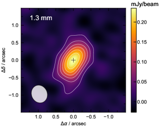
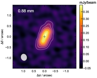
Figure 1: ALMA 1.32 and 0.88 mm continuum images of the HD110058 disk (left and right panels). Contour levels are shown at 3, 7, 14 ,21 times the RMS of each image (8  $\mu$Jy beam^-1 and 17 $\mu$Jy beam^-1 respectively). The position of the star is indicated with a black plus symbol. The integrated fluxes reported in Table 2 were integrated within a circular region centered at the star position of $1.0\arcsec$ in radius. The ellipse in the lower left represents the synthetic beam of the data.

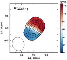
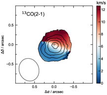
Figure 2: ¹²CO (2$-$1) and ¹³CO(2$-$1) moment 0 and moment 1 maps of HD110058 (left and center panels, respectively). Colored maps show the velocity centroids for each pixel, i.e. moment 1. Contours show integrated intensity of line emission. First contour is 3 times the RMS noise and each subsequent contour level increases with a step of 3$\times$RMS (i.e. contour levels are 3, 6, 9, 12, and so on, times the RMS). The corresponding RMS noise for the zeroth moment are listed in Table 2. Right: Radial distribution of 1.33 mm continuum, ¹²CO (2$-$1) and ¹³CO (2$-$1) obtained from spatially integrating the continuum and moment 0 images along a line perpendicular to the major axis of the disk. The profiles have been normalised to unity for comparison. The blue region shows the projection of the synthesized beam size in the direction of the disk’s major axis.

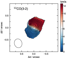
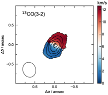
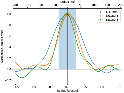
Figure 3: ¹²CO(3$-$2) and ¹³CO(3$-$2) moment 0 and moment 1 maps of HD110058 (left and center panels, respectively).Colored maps show the velocity centroids for each pixel, i.e. moment 1. Contours show integrated intensity of line emission. First contour is 3 times the RMS noise and each subsequent contour level increases with a step of 3$\times$RMS (i.e. contour levels are 3, 6, 9, 12, and so on, times the RMS). The corresponding RMS noise for the zeroth moment of ¹²CO(3$-$2) and ¹³CO(3$-$2) are 3.4, and 4.9 mJy beam^-1 km s^-1, respectively. Right: Radial distribution of 0.88 mm continuum, ¹²CO (3$-$2) and ¹³CO (3$-$2) obtained from spatially integrating the continuum and moment 0 images along a line perpendicular to the major axis of the disk. The profiles have been normalised to unity for comparison. The blue region shows the projection of the synthesized beam size in the direction of the disk’s major axis.

3.1 Continuum and line images

Figure 1 shows the 1.3 and 0.8 mm continuum images of the edge-on disk around HD 110058. The disk is resolved in both images. The radial surface brightness profiles (averaged in the direction perpendicular to the major axis) of the continuum images are shown in the right panels of Figure 2 and Figure 3. The band 7 image shows a 1-dimensional slice along the disk’s major axis. The surface brightness profile suggests the two peaks of an edge-on ring are marginally resolved. The northwest peak appears brighter than the one located towards the southeast, but not at a significant level. The band 6 continuum profile peaks at the star’s position, without any notable features, due to the lower spatial resolution.

The total integrated continuum fluxes at 1.32 and 0.88 mm are 0.51$\pm$0.05 mJy and and 1.39$\pm$0.16 mJy respectively, integrated within a $1.0$″radius centered at the position of the star. The error bars in the derived fluxes include the statistical errors and ALMA’s 10% nominal absolute flux calibration accuracy in bands 6 and 7 (see Table 2). The spectral index between the two frequencies is 2.5 $\pm 0.4$, consistent with the flux reported at 239.0 GHz by Lieman-Sifry et al. (2016) within uncertainties.

We use the CASA task imfit to fit a 2D Gaussian to the continuum data. Table 2 presents the source properties derived from the Gaussian fitting at each frequency. The disk is resolved in both directions in both bands. The deconvolved Gaussian size in the direction of the major axis of the disk is 0.77″($\sim$100 au), while the deconvolved size perpendicular to this is 0.2″ ($\sim$26 au). The inclination of the disk derived from the ratio of the minor and major axis (assuming a flat circular disk/ring) is $\sim$75^∘ in both bands. This inclination is quite different from the near-IR images showing a disk very close to an edge-on orientation. In Section 4.1 we do a more formal derivation of the disk’s inclination, and discuss its implications in Section 5.2.

Figure 2 and Figure 3 show the moment 0 (contours) and moment 1 (colorscale) images for the observed transitions of ¹²CO and ¹³CO. The disk is detected in all lines. The source properties are listed in Table 2. Integrated fluxes are reported in Table 2, and were integrated within a circular region centered at the position of the star of $0.65\arcsec$ in radius. The ¹²CO(2$-$1) integrated flux of 90.6 $\pm$ 12.0 mJy km s^-1 is consistent with the values reported in previous, lower-resolution, ALMA observations (92 $\pm$ 17 mJy km s^-1, Lieman-Sifry et al., 2016). The moment 1 maps show the typical velocity field of a disk in Keplerian rotation, which is also clear in the position-velocity (PV) diagrams (see Appendix A). Similarly to Matrà et al. (2017a), we also computed PV for the line ratios, and also for the consequential optical depth using the (2-1) and (3-2) transitions separately. These are also shown in Appendix A. The integrated spectra for both transitions of both isotopologues, and the derived optical depths per channel, are also shown in the appendix. The resulting optical depths (calculated assuming an interstellar 12C/13C abundance ratio of 76; Wilson & Rood, 1994) indicate that the disk is optically thick in both transitions. This is consistent with the fact that the ¹²CO and ¹³CO fluxes are roughly the same, suggesting the ¹²CO emission is highly optically thick. Also, the ratio of the (3-2) to (2-1) fluxes goes roughly as $\nu^{2}$, which also suggests the emission is optically thick.

The 1-dimensional radial surface brightness profiles of ¹²CO and ¹³CO are shown in Figure 2 and Figure 3. Compared to the dust disk, the gas disk is more compact.

The 2D Gaussian fit of the moment 0 maps from imfit suggests that the gas disk is marginally resolved along the minor axis in ¹³CO(2-1) and ¹²CO(3-2). This would indicate that this disk is not perfectly edge-on, and its inclination is slightly lower than $90^{\circ}$. To verify whether the ¹²CO(3-2) disk is truly resolved in the direction of the disk’s minor axis we computed normalized intensity profiles in the direction of the disk’s minor axis. We compared the FWHM of the profiles to the FWHM of the projected beam size, and conclude that the ¹²CO(3-2) gas disk is only marginally resolved in the direction of the minor axis. We, therefore, refrain from using the moment 0 maps to obtain information on the basic gas disk properties, and instead in Section 4.2 we use full radiative transfer modeling to obtain the disk’s parameters such as inclination and radius.

4 Radiative transfer models

In this section, we use radiative transfer codes to fit the continuum and spectral line visibilities in order to constrain the distribution of dust and gas in this system. To fit the continuum data, we use the python package disc2radmc (Marino et al., 2022) that allows to create disk models and uses RADMC-3D (Dullemond et al., 2012) to compute synthetic images. These images are then used to calculate model visibilities and a $\chi^{2}$ as in Marino et al. (2018). Note that we rescale the visibility weights of each band separately by a factor such that the reduced $\chi^{2}$ of our best fit model is equal to 1 (Marino, 2021). This is to ensure the uncertainty estimates are correct. The line data is modeled using the pdspy code from Sheehan et al. (2019).

4.1 Dust ring model

Table 3: Best fit parameters of the ALMA continuum data using the parametric model in §4.1.

Parameter	Best fit value	description
$M_{\mathrm{dust}}$ [ M⊕]	$0.080_{-0.003}^{+0.002}$	Total dust mass
$r_{c}$ [au]	$31_{-8}^{+10}$	Disk peak radius
$\Delta r_{\rm in}$ [au]	$26_{-18}^{+26}$	Inner FWHM
$\Delta r_{\rm out}$ [au]	$72_{-12}^{+9}$	Outer FWHM
$h$	$0.17^{+0.05}_{-0.09}$	Vertical aspect ratio
$i$ [∘]	$78^{+7}_{-3}$	Disk inclination from face-on
PA [∘ ]	$157\pm 1$	Disk position angle
$\alpha_{\mathrm{mm}}$	$2.45\pm 0.06$	Spectral index

Note. — The values correspond to the median, with uncertainties based on the 16th and 84th percentiles of the marginalized distributions.

The dust disk is modeled as an axisymmetric ring with a surface density following an asymmetric Gaussian distribution

$$\Sigma_{\rm dust}(r)=\Sigma_{c}\begin{cases}\exp[-\frac{(r-r_{c})^{2}}{2\sigma_{\rm in}^{2}}]&\text{if $r\leq r_{c}$},\\ \exp[-\frac{(r-r_{c})^{2}}{2\sigma_{\rm out}^{2}}]&\text{if $r>r_{c}$},\end{cases}$$ (1)

where $\sigma_{\rm in,out}$ are the standard deviations interior and exterior to the surface density peak at $r_{c}$. Vertically, the disk is assumed to have a Gaussian distribution with a standard deviation $H(r)$, which is equivalent to assuming a Rayleigh distribution of inclinations (Matrà et al., 2019). The model free parameters are the total dust mass ($M_{\rm d}$), the peak radius ($r_{c}$), the inner and outer full width half maxima ($\Delta r_{\rm in,out}$), its vertical aspect ratio ($h$, where $h=H/r$ is constant across the disk), the disk inclination ($i$), its position angle (PA), the disk spectral index ($\alpha_{\rm mm}$) and phase centre offsets for both band 6 and 7 observations. We leave $h$ as a free parameter since this disk is highly inclined and the minor axis resolved, and thus these observations could provide good constraints. We use uniform priors for all the free parameters, restricting $h$ to values in the range $0.015-0.4$ for computational reasons. The dust grain properties are the same as in Marino et al. (2018), dust species with a mass weighted opacity assuming a size distribution from 1 $\mu$m to 1 cm, with a power-law index of -3.5, and made of a mix of astrosilicates, amorphous carbon and water ice. This choice only has an effect on the dust opacity and derived mass, but not on the dust distribution. The stellar radius was fixed to 1.6  R_⊙ and the stellar temperature to 8000 K, consistent with the system’s parameters (Saffe et al., 2021). These parameters determine the dust temperature (calculated with RADMC-3D) and stellar flux in bands 6 and 7 (2 $\mu$Jy and 5 $\mu$Jy, respectively, below our observations’ detection limit).

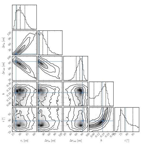
Figure 4: Posterior distribution obtained for the disk peak radius, inner and outer FWHM, vertical aspect ratio, and inclination. The blue lines show the parameter values that give the best fit, whereas the vertical dashed lines show the 16th, 50th and 84th percentiles. The contours represent the 68, 95 and 99.7% confidence levels.

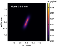
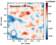
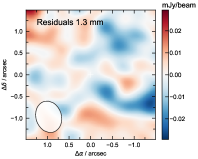
Figure 5: Left: Band 7 best-fit dust ring model image. Center: Band 7 residual image after subtracting the model to the data. Color stretch ranges from -3$\sigma$ to 3$\sigma$, where $\sigma$ = RMS of 1.7$\times 10^{-2}$ mJy beam^-1. Right: Band 6 residual image after subtracting the model to the data. Color stretch ranges from -3$\sigma$ to 3$\sigma$, where $\sigma$ = RMS of 8.6$\times 10^{-3}$ mJy beam^-1.

The parameter space is explored using a Markov Chain Monte Carlo (MCMC) routine. For each set of parameter values, disc2radmc is used to compute the dust density distribution and RADMC-3D to compute a synthetic image at 0.88 mm, which is then used to calculate an image at 1.3 mm based on a uniform disk spectral index $\alpha_{\rm mm}$ that is left as a free parameter These model images are multiplied by the corresponding ALMA primary beam, and finally fourier transformed to produce model visibilities that can then be compared to the data. The Band 6 and Band 7 data were fitted simultaneously using the full aggregate bandwidth from all line-free channels. The posterior distribution is constrained using the Goodman & Weare’s Affine invariant MCMC Ensemble Sampler in the emcee code (Foreman-Mackey et al., 2013). The best-fit parameters for the dust ring model are presented in Table 3 and the posterior distribution of the most relevant parameters in Figure 4.

These results indicate the disk is centered at $31^{+10}_{-8}$ au with an inner edge that is sharper than the outer edge (i.e. $\Delta r_{\rm in}<\Delta r_{\rm out}$). Defining the disk inner edge location as r_c-$\Delta r_{\rm in}$/2, and outer edge location as r_c+$\Delta r_{\rm out}$/2, we find that the disk inner edge is at $18_{-4}^{+3}$ au (smaller than 23 au at 99.7% confidence) and its outer edge is at $67\pm 4$ au (larger than 59 au at a 99.7% confidence). Since the mm-sized dust traces the planetesimal distribution, these observations thus reveal that the planetesimals are distributed in a 49 au wide belt with a fractional width (disk width over its disk centre) of 1.2 or 1.6 depending on the definition of its disk centre. This is anyway much higher than the median fractional width of debris disks observed with ALMA of 0.7 (Matrà et al. in prep). The derived outer radius of ${\sim}70$ au is consistent with the estimate from Lieman-Sifry et al. (2016). The inner radius of the dust ring is inferred for the first time, although its exact value is likely dependent on the assumption of a Gaussian density distribution. Higher resolution observations would be needed to determine this with confidence. Nevertheless, as part of a separate project (Terrill et al. in prep), we explored that when using a non-parametric model we find a radial profile that peaks at around 30 au, with a smooth outer edge. This is consistent with our model choice of a simple Gaussian profile, allowing for the inner and outer regions to have different widths/standard deviations.

Consistent with scattered light observations, the disk is found to be very inclined although the marginalized distribution is still consistent with a wide range of values from $90^{\circ}$ (perfectly edge-on) down to 71^∘ (99.7% lower limit). This behavior is due to the disk being resolved along the minor-axis, thus if the disk is vertically thin (low $h$), the inclination must be below ${\sim}80^{\circ}$ to account for the minor-axis width. This also explains the correlation between $h$ and the inclination in Figure 4, with high values of $h$. Interestingly, scattered light observations and our gas modelling presented below suggest the disk to be very inclined ($i>80^{\circ}$), which would suggest the disk is vertically resolved with $h=0.13-0.28$ (99.7% confidence interval). In §5.2 we discuss this finding and its implications.

4.2 Gas disk model

To provide more formal constraints on the gas disk properties, we use the pdspy code from Sheehan et al. (2019) to fit the ¹²CO and ¹³CO emission. The code generates synthetic line emission maps that can be readily compared to the data. It uses RADMC-3D to produce synthetic line emission maps which are then sampled similarly to the visibility data using the fast sampling code GALARIO (Tazzari et al., 2017). The synthetic model visibilities are compared to the data using a Bayesian approach in which the probability distribution is sampled via Markov Chain Monte Carlo (MCMC) method implemented in the emcee code.

The model assumes a passively irradiated disk in hydrostatic equilibrium rotating with a Keplerian velocity field (the vertical and radial velocities are zero). The radial surface density of the disk is given by the standard Lynden-Bell & Pringle (1974) profile, which corresponds to a power-law disk with an exponentially decaying tail at large radii,

$$\Sigma(r)=\Sigma_{\rm 0}\left(\frac{r}{R_{\rm c}}\right)^{-\gamma}\exp\left[-\left(\frac{r}{R_{\rm c}}\right)^{2-\gamma}\right].$$ (2)

The characteristic radius R_c represents the radius where the exponential tail starts to dominate the density profile, and is a proxy for the outer radius of the disk. The power-law surface density exponent $\gamma$ also controls how sharply the disk is truncated in the exponential tail. The reference surface density $\Sigma_{\rm 0}$ is related to the total disk mass M_disk as

$$M_{\rm disk}=\frac{2\pi R_{c}^{2}\Sigma_{\rm 0}}{2-\gamma}.$$ (3)

We assume that the disk is vertically isothermal, with the radial temperature distribution of the gas is defined by a power-law

$$T(r)=T_{0}\Big{(}\frac{r}{1\ \mathrm{au}}\Big{)}^{-q}.$$ (4)

Solving for hydrostatic equilibrium, the vertical scale height as a function of radius is

$$H(r)=\left[\frac{k_{B}\,r^{3}\,T(r)}{G\,M_{*}\,\mu m_{H}}\right]^{1/2},$$ (5)

where M_∗ is the mass of the central star, $\mu$ is the mean molecular weight of the gas, and k_B and G are Boltzmann’s and gravitational constants, respectively. The code considers local thermodynamic equilibrium (LTE) to generate the images, which is valid if the gas densities are high enough. We assume $\mu=14$, which corresponds to the case where the gas is predominantly composed of carbon and oxygen atoms released by photodissociation of CO (Kral et al., 2016).

The model adopted here includes the following free parameters: total disk mass M_disk, stellar mass M_∗, disk characteristic radius $R_{\rm C}$, disk inner radius $R_{\rm in}$ (inside of that location the density drops to zero), T₀ (the temperature at 1 au), position angle PA, the surface density power law exponent $\gamma$, the system’s radial velocity v_sys (LSRK), and offset from the phase center x₀ and y₀. The dynamical mass of the central object M_∗ is fitted assuming the distance of 129.9 pc (Gaia Collaboration et al., 2018). The radial exponent for the temperature dependence $q$ is fixed to 0.5. The ¹³CO isotopologue ratio with respect to ¹²CO was set to the canonical value of 76 (Wilson & Rood, 1994).

We chose to fit the ¹²CO(3-2), ¹³CO(3-2) and ¹³CO(2-1) data simultaneously to exploit the higher angular resolution of the Band 7 data while still using the (2-1) lines of ¹³CO to solve for the temperature/mass degeneracy. We found that adding the extra ¹²CO(2-1) made the running time of the fit prohibitively large.

The MCMC run started with 100 walkers, which were left to evolve during 1100 steps for the burn-in phase. Following this burn-in phase, the MCMC code ran for another 2000 iterations to sample the posterior probability distribution. The resulting best-fit parameters and uncertainties are presented in Table 4. We report the maximum likelihood model from our fit as the best-fit parameters, and use the range around the best fit parameter values including 95% of the posterior samples to report the uncertainties on these values. We choose to report the 95% confidence intervals here because the posteriors for some parameters from the fit are highly skewed, with the maximum likelihood value falling outside of the 68% confidence interval. The marginalised probability distributions are presented in Figure 6.

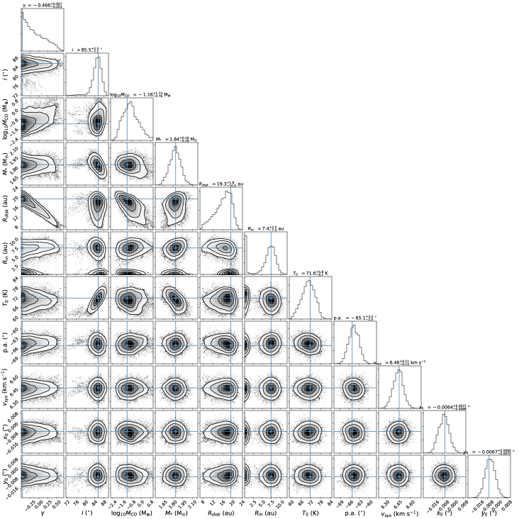
Figure 6: Triangle plots of the posterior probability distribution function for the gas disk model that fits ¹²CO(3-2), ¹³CO(3-2), and ¹³CO(2-1) simultaneously. The blue lines show the point with the highest probability, i.e. the most likely model from the fit. The maximum likelihood values and uncertainties corresponding to the range around these values including 95% of all walkers in the posterior are shown at the top of each column.

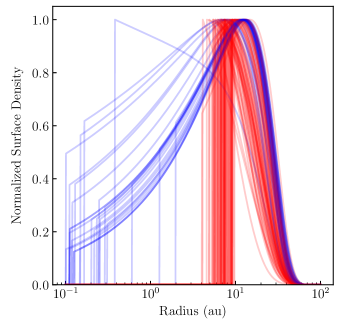
Figure 7: Normalized CO surface density distribution from the MCMC run. Coloring is based on R_in $<$ 3 au (blue) and R${}_{in}>$3 au (red) from the two ’best-fit’ solutions.

The disk inclination of $85.5_{-7.2}^{+2.5}$ determined for the gas disk is compatible with the disk being very close to edge-on. It is also consistent with the inclination derived for the mm dust disk. The stellar mass of 1.84${}_{-0.18}^{+0.16}$ M_⊙ is well constrained, with minimal dispersion, and is in better agreement with the star being late A- dwarf, closer to A6/7. This revised stellar classification seems consistent with recent derivation of the stellar temperature of T$\sim 7839\pm 202$ K from optical spectroscopy (Saffe et al., 2021), which also suggest that HD 110058 is an A6/7V star rather than A0V (Pecaut & Mamajek, 2013). The determined system’s radial velocity of $6.4~{}\pm 0.1$ km s^-1 is consistent with the heliocentric velocity of $\sim$ 12.6 km s^-1 measured in the optical (Hales et al., 2017; Rebollido et al., 2018) after converting to LSRK (5.6 $\pm 2.4$  km s^-1) . The position angle reported by the fit uses the RADMC-3D convention, i.e., the position angle of the angular momentum vector of the disk on the plane of the sky, which is offset by 90 degrees from the position angle defined by the disk’s major axis. (see Czekala et al., 2019). Therefore the result for the gas position angle in the traditional convention is 155.1${}_{-2.5}^{+3.5}$^∘, in agreement with the $157\pm 1$^∘ position angle derived for the mm dust disk (Section 4.1), and the $155\pm 1$^∘ measured in scattered light (Kasper et al., 2015).

The most relevant parameters to constrain the origin of the carbon monoxide present in the disk are the disk’s inner and outer radius, the total CO mass and the resulting surface density distribution. The total CO mass present in the disk as derived from the fitting of the ¹²CO(3-2), ¹³CO(3-2) and ¹²CO(2-1) data is $0.069^{+3.56}_{-0.057}$  M_⊕. Even taking the lower end of the 95% confidence interval, this is more than two orders of magnitude larger than the CO mass estimated by (Kral et al., 2017) using a disk model that accounts for optical thickness and non-LTE, and three orders of magnitude larger than CO mass derivations based on previous ¹²CO(2-1) data that assume optically thin emission (e.g., Moór et al., 2017). We note, however, that this mass is derived under the assumptions of the model that we employ, and this difference could be in part due to systematic effects related to our relatively simplistic choice of model. For example, we assume the disk is vertically isothermal, though this is almost certainly not the case, in LTE, and assumes that the surface density profile can be well approximated by a tapered power law. If any of these assumptions are incorrect, it could have an effect on the mass we derive. Including such additional physics (e.g., Rosenfeld et al., 2013) and alternative surface density distributions in future modeling could potentially alter this picture.

The disk’s characteristic radius R_c derived from the fit is 19.3${}_{-10.5}^{+1.8}$ au, which confirms that the gas disk is more compact than the dust disk that has an outer edge of 70 au. We discuss this difference in §5.3.

We find that $R_{\rm in}$ is not well constrained, showing a bimodal distribution corresponding to two solutions: $R_{\rm in}$ smaller or larger than ${\sim}3$ au. That said, while the inner edge of the disk itself is not well constrained, we do find that these two families of solutions provide a consistent picture of where the CO gas is located. Figure 7 presents the normalized surface density profiles for a random sample of the posterior distribution, colour-coded by $R_{\rm in}$: blue for $R_{\rm in}<3$ au and red otherwise. From this figure, we can see how most solutions with small $R_{\rm in}$ (blue) have surface densities that increase with radius up to $R_{\rm c}$, effectively creating a cavity depleted of CO gas. Solutions with a large $R_{\rm in}$ tend to converge to $R_{\rm in}\sim 7$ au. We also note that though the posterior for R_in is bimodal, this could in part be due to our choice of prior on $\gamma$. $\gamma$ controls the surface density profile, with negative values of $\gamma$ leading to the smoothly increasing surface density profiles for the solution with $R_{\rm in}<3$ au. More negative values of $\gamma$ lead to more sharply increasing surface density profiles that more closely approximate the truncated disk solution, which could in turn plausibly have larger values of $R_{\rm in}$. In our modeling, we place a limit of $\gamma>-0.5$, however lowering this limit could potentially thereby fill in the gap between the two modes of the posterior that we see.

Hence, although we cannot place a strong constraint on where the formal inner edge of the disk is, both solutions suggest that the CO surface density profile peaks near $\sim 10$ au and has a depletion of material within that radius. We further note that gas at radial distances smaller than 10 au should result in gas emission at velocities larger than 10 km s^-1, but such emission is not visible at a significant level in Position-Velocity diagrams of the data nor of the best-fit model (see Appendix A). Higher spatial resolution and sensitivity data is required to determine in more detail the surface density profile of the CO gas.

We note that the temperature at 1 au (T₀) found by the modeling, of $71^{+5.7}_{-9.1}$ K, is seemingly quite small for the proximity to an A0 star. That said, 1 au is well below the limits of our observations, and as Figure 7 shows, we also find a dearth of material at that radius. As such, we suspect that the low temperature is likely the result of the model matching the temperature at larger radii that are probed by our observations, and extrapolating inwards using the fixed temperature power-law exponent ($q=0.5$), rather than a true estimate of the disk temperature at 1 au. We note that the temperature at 1 au ($T_{0}$) corresponds to a temperature of $\sim 16$ K at 20 au where the gas density peaks. This temperature seems low for the proximity to an A-type star. This may, however, once again be due to our relatively simple choice of model (or if the gas is in non-LTE and $T$ different from $T_{\rm ex}$). The temperature controls the height of the disk, and so the low temperature may be required to match the geometric profile of the disk. A more physically motivated model with a cold disk midplane and a warm atmosphere (e.g., Rosenfeld et al., 2013), or a CO vertical distribution skewed towards the midplane due to photodissociation (Marino et al., 2022), may better match the expected temperature of the disk at this radius while also producing the proper height of the gas disk.

Table 4: Best-fit Gas Disk Model Parameters

Parameter	Best fit value	description
$\gamma$	$-0.47_{-0.02}^{+0.95}$	disk CO surface density exponent
Incl [∘]	$85.5_{-7.2}^{+2.5}$	disk inclination from face-on
$\log_{10}$(MCO) [ M⊕]	$-1.16_{-0.77}^{+1.72}$	total CO mass
Mstar [M⊙	$1.84_{-0.18}^{+0.16}$	Stellar Mass
Rdisk [au]	$19.3_{-10.5}^{+1.8}$	Disk Characteristic Radius (RC)
Rin [au]	$7.4_{-7.3}^{+2.2}$	Disk inner Radius
T0 [K]	$71.6_{-9.1}^{+5.7}$	Temperature normalization, at 1 au
PA [∘]	$-65.1_{-2.5}^{+3.5}$	Position angle of the disk’s angular momentum vector
vsys [km s-1]	$6.46_{-0.13}^{+0.11}$	Systemic Velocity in LSRK
x0 [″]	$-0.0064_{-0.0086}^{+0.0071}$	X- Offset
y0 [″]	$-0.0067_{-0.0071}^{+0.0091}$	Y- Offset

Note. — The best-fit values corresponds to points with the highest probability (i.e. the the maximum likelihood model from the fit) and the 95% confidence interval around that point.

5 Discussion

In this section we discuss the results regarding the vertical extent of the disk derived in §4.1, and the CO gas distribution derived in §4.2.

5.1 Dust radial distribution

The new ALMA data resolve the circumstellar dust around HD 110058 and provide better constraints on the disk’s parameters compared to previous observations from Lieman-Sifry et al. (2016) which had resolution of $1.3\arcsec\times 0.8\arcsec$ (a factor of 3-4 lower than our new observations). The analysis of the new data strongly suggests that the dust (and thus planetesimal) disk is very wide with a FWHM of 49 au and a peak radius of 31 au. We note that this disk has a very small peak radius compared to other bright debris disks around stars of similar luminosity observed with ALMA (expected central radius of $110\pm 20$ au; Matrà et al., 2018). The only disk that appears to be similar is HD 121191, with a central radius of 52 au and width smaller than 61 au (Kral et al., 2020). HD 110058’s disk being smaller could be an effect of its short age ($\sim 17$ Myr old), meaning that the inner regions would be less depleted than in older systems due to collisional evolution. However, other young disks around similar luminosity stars like the ones around $\beta$ Pic, HD 131488, HD 131835 are all significantly larger (Matrà et al., 2019; Moór et al., 2017; Kral et al., 2019). Thus it appears that this system is at the tail of the radius distribution for bright debris disks. In scattered light the disk is also seen small with signal detected to only about 65 au (Kasper et al., 2015; Esposito et al., 2020), location that is consistent with our inferred disk outer edge.

The disk inner edge is 18 au ($<23$ au at 99.7% confidence), which is the smallest inferred inner edge inferred for an exoKuiper belt with ALMA (Matrà et al. in prep). This has strong implications for the evolution of gas, since the equilibrium temperature would be higher than 100 K and thus other volatiles apart from CO would readily sublimate (e.g. CO₂ Collings et al., 2004). CO₂ sublimation could trigger an increase in outgassing, and since this molecule quickly photodissociates into CO (Hudson, 1971), this would enhance the CO gas production rate in the inner regions.

5.2 Dust vertical distribution

Our observations strongly suggest that the disk is vertically thick, with an aspect ratio in the range 0.13-0.28 (99.7% confidence) if $i>80^{\circ}$ (i.e. consistent with the gas and scattered light observations). The vertical thickness of debris disks is a key property that traces the inclination dispersion, and thus it contains valuable information about the dynamical history of a system. So far, this has been inferred for two edge-on disks (Matrà et al., 2019; Daley et al., 2019) and a few less inclined disks (Marino et al., 2019; Kennedy et al., 2018). These measurements of $h$ range between $0.02-0.09$, which translate to inclination dispersions ($i_{\rm rms}$) of $2-7^{\circ}$ ($i_{\rm rms}=\sqrt{2}h$, Matrà et al., 2019) that are close to the inclination dispersion of the cold population of the classical Kuiper belt ($\sim 3^{\circ}$, Brown, 2001). $\beta$ Pic is an exception to this as it was found to be best fit with a double population that is analogous to the classical Kuiper belt (Matrà et al., 2019). These populations have inclination dispersions of $1^{\circ}$ and $9^{\circ}$. For HD 110058 we concluded that the inclination dispersion is likely in the range $11-23^{\circ}$, which would make it the thicker disk known to date, but still lower or consistent with the classical Kuiper belt’s hot population and scattered disk ($20-30^{\circ}$ Brown, 2001).

5.2.1 Scattering

This high degree of orbital stirring revealed by the high $i_{\rm rms}$ strongly suggests that this disk has been perturbed by planets. The level of stirring is a combination of the mass and number of stirrers (since stirring is localized), which raise the relative velocities over time. Following a similar procedure to Matrà et al. (2019) we can estimate the minimum planet mass that could cause this stirring through close encounters. We first use their equation 10 to find that the relative velocities are in the range 3-7 km s^-1 at the peak radius. In order to reach these relative velocities, the massive bodies stirring the disk should have escape velocities close or higher to those values, and thus we find the minimum stirrer mass as

$$M_{\rm s}=0.03M_{\oplus}\left(\frac{h}{0.13}\right)^{3}\left(\frac{r}{\rm 31\ au}\right)^{-3/2}\left(\frac{M_{\star}}{1.8\ M_{\odot}}\right)^{3/2}\left(\frac{\rho}{\rm 4\ g\ cm^{-3}}\right)^{-1/2},$$ (6)

where $\rho$ is its bulk density and $r$ the orbital radius. Therefore, the stirrer should at least be as massive as Mercury.

However, using equations 12 and 14 from Matrà et al. (2019), we find that a planet with this minimum mass would be unable to stir the orbits to the observed levels on its own within the age of the system (17 Myr versus $\sim$ 500 Gyr that it would take to stir the system to this level on its own), and thus an unrealistic number of these planets closely packed would be needed to stir the disk. More feasible is that the stirring was caused by multiple widely spaced planets with a larger mass. The intersection of equations 12 and 14 in Matrà et al. (2019) sets the minimum planet mass for which stirring can be achieved by the age of the system and planets are spaced by $\sim 14$ Hill radii, ensuring stability and also stirring in between their orbits. For HD 110058, we find that minimum mass is 15 $M_{\oplus}$. Such planets could be embedded in the disk and have cleared gaps ($>5$ au, Wisdom, 1980) that our observations are unable to resolve yet (Marino et al., 2018, 2019, 2020; MacGregor et al., 2019).

Alternatively, the high inclinations could be due to a single massive planet near the disk inner edge. Such planet could have scattered most of the original population while migrating, in which case the disk would be dominated today by a population similar to the Kuiper belt’s scattered disk, but much more massive (Duncan & Levison, 1997). Our modelling indeed suggests that surface density beyond the peak radius decays smoothly with radius as expected if the disk is highly stirred (Marino, 2021). Higher resolution observations could constrain better the location of the disk inner edge and the surface density profile, and thus constrain better this scenario.

5.2.2 Secular perturbations

A different mechanism that could explain the high $i_{\rm rms}$ is through secular interactions. If the disk was initially misaligned to an inner massive planet, the disk would have been forced to the same orbital plane as the planet (Wyatt et al., 1999). This has been suggested to explain the warp in $\beta$ Pic (Mouillet et al., 1997; Augereau et al., 2001). As the disk particles interact with the planet, their inclinations precess and after one secular timescale they form a thick disk with a vertical height equal to twice the initial mutual inclination between the disk and planet. Thus the derived inclination dispersion of $11-23^{\circ}$ would suggest an initial misalignment of $6-12^{\circ}$. Interestingly, this system shows a tentative warp in its outer regions (Kasper et al., 2015). Warps are expected during this type of evolution. As the secular timescale increases with radius for an internal perturber, beyond a certain radius ($a_{w}$) disk particles will have not precessed enough to be aligned with the orbit of the planets. The location where this happens thus can constrain the mass and semi-major axis of the perturbing planet. Using Equation 4 from Dawson et al. (2011), we find that a warm exo-Jupiter at 3-10 au that was born misaligned or evolved to a misaligned orbit could explain the warp location. If the planet semi-major axis ($a_{p}$) is much smaller than the warp location, their equation 4 can be simplified and the planet mass can be approximated by

$$M_{p}=0.8M_{\rm Jup}\left(\frac{\tau}{\rm 10\ Myr}\right)^{-1}\left(\frac{a_{p}}{\rm 10\ au}\right)^{-2}\left(\frac{a_{w}}{\rm 50\ au}\right)^{7/2}\left(\frac{M_{\star}}{1.8\ M_{\odot}}\right)^{1/2}.$$ (7)

Figure 8 shows the planet mass as a function of semi-major axis to create a warp at 40 (blue) and 60 au (orange) after 10-17 Myr of secular interactions. Since the location of the warp is not well constrained, we use 40 and 60 au as a reasonable range consistent with the tentative warp reported by Kasper et al. (2015). Unfortunately, current limits for this system are poor and only rule out planets more massive than $\sim 8$ $M_{\rm Jup}$ at 50-300 au projected separations (Wahhaj et al., 2013; Meshkat et al., 2015). Similarly, this system does not show a significant proper motion anomaly when comparing Hipparcos and Gaia eDR3 astrometry (Brandt, 2021; Kervella et al., 2022). Since this system is edge-on, these limits do not rule out the presence of a massive companion in the system at 1-20 au semi-major axes.

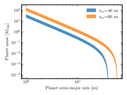
Figure 8: Planet mass and semi-major axis required to produce a warp at 40 (blue) or 60 au (orange). The width of the lines account for a secular evolution during 10-17 Myr.

Finally, it is also interesting to compare the vertical distribution of small dust. Although Kasper et al. (2015) and Esposito et al. (2020) did not constrain the vertical distribution of small dust, the disk appears to be flatter than in the ALMA observations that trace the large dust. Small grains having a smaller inclination dispersion could be a result of damping collisions (Pan & Schlichting, 2012) or even gas drag as the dimensionless stopping time (Stokes number) of $\mu$m-sized grains could be close to 1 (see §5.3). Forward modelling of scattered light observations is needed to constrain the vertical distribution of small dust and confirm this difference in vertical distributions. It is also possible that the distribution of small grains appears flatter due to the reduction methods to subtract the stellar PSF, which can affect the observed morphologies.

5.3 CO gas distribution

The observations confirm the gas detection from Lieman-Sifry et al. (2016), and detect all four targeted carbon monoxide isotopologue transitions. Since gas is released from solid bodies (if secondary), they should be roughly co-located. We find that the CO gas emission is notoriously more compact, spanning between r$\sim 1-10$ au out to 30 au, but with a peak radius at 10-20 au that is still consistent with the dust peak radius ($31_{-8}^{+10}$ au). The different distributions of the CO gas and dust is not unexpected. Models of gas-rich debris disks show that the gas can viscously expand, reaching regions closer in and further out unless the viscosity is very low (Kral et al., 2019; Marino et al., 2020). However, these models also show a sudden drop in the surface density of CO beyond a critical outer radius where the carbon surface density drops to levels in which it does not shield CO effectively from photo-dissociation by interstellar UV. This destroys CO molecules at large radii where column densities are low.

In order to test if the gas and dust distributions can be reconciled in a secondary origin scenario, we use exogas (Marino et al., 2020, 2022) to model the radial evolution of gas released from the planetesimal belt. We consider a star with a mass of 1.8 M_⊙, luminosity of 9 L_⊙, surrounded by a belt of planetesimals with a surface density that peaks at 22 au and with inner and outer FWHM’s of 6 and 82 au. Note that these are the parameters that give the best fit to the continuum data and are slightly different from the medians presented in Table 3. CO gas is input at a rate of $4\times 10^{-3}\$M${}_{\oplus}/$Myr (consistent with its fractional luminosity of $\sim 10^{-3}$ and a CO mass fraction of 10% in planetesimals, Matrà et al., 2017b), and we evolve the gas for 10 Myr (a rough estimate of the period over which CO has been released after the protoplanetary disk dispersal) considering CO photodissociation, shielding by CO and CI, viscous spreading, and radial diffusion. We assume CI and CO are segregated with CI mainly present in a surface layer surrounding the CO gas creating optimal shielding (analogous to assuming negligible vertical diffusion Marino et al., 2022). In addition, we update exogas such that the release rate of CO gas is also inversely proportional to the orbital period ($\dot{\Sigma}_{\rm CO}^{+}\propto\Sigma_{\rm dust}^{2}\Omega_{\rm K}$ with $\Omega_{\rm K}$ with the Keplerian frequency, Wyatt et al., 2007). This enhances the CO release at smaller radii. Finally, we neglect the stellar UV in the CO photodissociation calculations. In reality, the stellar UV flux for this A-type star will be higher than the ISRF at the distances considered. However, we expect that the CO photodissociation at the gas disk inner edge will quickly form an optically thick CI layer in the radial direction that will shield the CO beyond that radius. It is important to note that selective photodissociation could reduce the abundance of ¹³CO during both the protoplanetary disk stage (while CO ices form, e.g. Miotello et al., 2014) and the debris disk stage (while CO is released from solids; Moór et al., 2019; Cataldi et al., 2020). Since the optical depth and mass are mainly constrained by the ¹³CO emission, a lower abundance would mean that the optical depth and mass of ¹²CO are even higher than estimated.

Figure 9 shows the evolution of the CO and CI gas for different viscosities (parametrized through $\alpha$). We find that CO can easily become shielded given the assumed CO released rate at the belt location. In order to fit the CO gas mass derived ($>10^{-2}~{}$M_⊕ at 95% confidence), $\alpha$ needs to be smaller or similar to 1$0^{-3}$. However, in order to explain the radial span of CO (10-30 au as highlighted by the vertical dashed lines) we find $\alpha\lesssim 10^{-4}$. Note that while CO extends out to 60 au, its density drops exponentially beyond its peak near 20 au due to the CO release rate that decreases with radius (represented by the grey shaded area) and the CO lifetime that decreases with radius due to the lower surface density of CO (i.e. lower self-shielding). Therefore, we conclude that the compact nature of the CO emission is consistent with the observed distribution of mm dust in a secondary origin scenario.

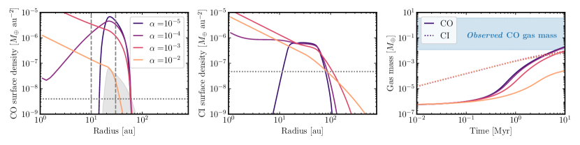
Figure 9: Simulated evolution of CO and CI undergoing viscous spreading and CO photodissociation using exogas. The surface density of CO and CI are shown in the left and middle panels for different viscosities after 10 Myr of evolution, while the right panel shows the temporal evolution of the total CO and CI mass. The vertical dashed lines in the left plot indicate the region where CO is significantly detected (10-30 au). The grey shaded region in the left panel represents the rate at which CO is released per unit area as a function of radius. The horizontal dotted lines in the left and middle panels represent the surface density above which CO starts to become self-shielded and shielded by CI. The blue shaded region in the right panel represents the CO mass derived from observations (95% confidence level).

In addition to the effects considered, there could be other factors that could make the release of CO gas even more enhanced at smaller radii. The higher temperature of solids at smaller radii could increase the release rate of CO (Jewitt et al., 2017), but also the release rate of CO₂, which can quickly photodissociate into CO+O and contribute to the CO gas (Lewis & Carver, 1983). These two effects would make the CO distribution appear even more compact as it would be heavily dominated by the innermost regions of the belt, perhaps matching even better the observations. Considering these effects is beyond the scope of this paper, but could be important when trying closely match the observations.

Finally, although we can fit the inner cavity in the CO gas distribution with a low viscosity, it is possible that the cavity exists due to a massive planet that is accreting most of the inflowing gas (Marino et al., 2020; Kral et al., 2020). Such a planet could be the same that is responsible for the dust large vertical thickness and tentative warp (§5.2).

5.4 Gas and dust interactions

The morphology of the small dust detected by the scattered light images could indirectly provide further information on the system’s total gas densities. If the gas densities are small, small dust is created where the mm dust is and extends further out due to radiation pressure. If the gas densities are high enough, small dust has Stokes numbers close to 1 and can migrate out very quickly due to gas-drag (Takeuchi & Artymowicz, 2001; Olofsson et al., 2022). This effect is the same radial drift that mm-sized dust experiences in protoplanetaty (Class II) disks. In this case, dust migrates out because small dust is even more sub-Keplerian than gas due to the effect of stellar radiation pressure , which is not the case of protoplanetary disks where the stellar radiation is completely blocked below the disk’s surface. If gas densities are even higher, the Stokes number would be $\ll$1, in which case the small dust would be coupled and will follow the gas as in a protoplanetary disk.

In order to quantify if this could be the case in HD 110058, we perform a similar analysis to the one in §5.6 in Marino et al. (2020) to estimate if radial migration could be important for the dynamics of small grains. Figure 10 shows the migration timescale from 20 to 30 au of the small grains at the blow-out limit ($\sim 2\mu$m) relative to their collisional lifetime as a function of the gas surface density. The red section of the line shows the densities that are ruled-out by our observations (at 95% confidence). If CO dominates the surface density over carbon and oxygen (as found in our model in §5.3), we expect that the gas density will be in the range $2\times 10^{-4}-7\times 10^{-2}$ g cm^-2 and thus the radial migration timescale relative to the collisional timescale will be smaller than one (green section). If this is the case, we would expect a pile up of small dust near the outer edge of the gas disk between 20-30 au before the density drops significantly. In this green section the smallest grains will have Stokes numbers close to 1 and thus will tend to settle towards the midplane as recently shown by Olofsson et al. (2022). Therefore, the scale height of small grains could be significantly smaller than the scale height of large grains. If the gas was primordial and thus dominated by other than CO (e.g. H or H₂), then the gas densities would be expected to be a factor $\geq 10^{3}$ higher than derived for CO, leading to densities above $\sim 0.1$ g cm^-2 (blue section). In this case the small dust grains are well coupled to the gas, decreasing its migration rate and settling towards the midplane (as in protoplanetary disks). In this high gas density regime gas drag could reduce the relative velocities of small grains and slow down the removal of unbound sub-blowout grains (Lecavelier Des Etangs, Vidal-Madjar, & Ferlet, 1998). Both effects could increase significantly the overall abundance of small grains and the disk fractional luminosity. The scattered light observations presented in Esposito et al. (2020) suggest that HD110058 may be reproduced by a disk with a moderately small aspect ratio, constant with radius, down to 16 au from the star. Unfortunately, Esposito et al. (2020) did not include HD 110058 in their disk morphology modelling of the scattered light images and we cannot confidently say anything conclusive from the images they provide. New SPHERE data (Stasevic et al. private communication) will provide a detailed analysis of the scattered light emission.

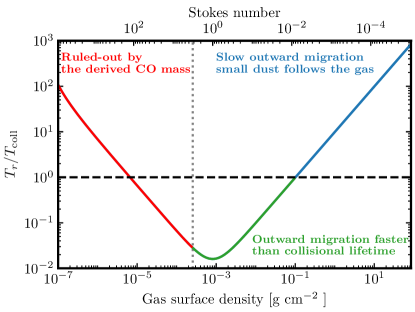
Figure 10: Radial migration timescale relative to the collisional lifetime of small grains as a function of gas surface density (solid line) following Marino et al. (2020) and using the derived parameters for HD 110058. The horizontal dashed lines represents a migration timescale equal to the collisional timescale. The vertical dotted line shows the minimum gas surface density derived from the minimum CO gas mass and radial distribution (95% confidence). The red section of the solid line represents the regime ruled out by our observations. The green section represents the region consistent with the CO observations and where the outward migration would be faster than the collisional timescale. The blue section represents the region where the gas density is high enough (and dominated by other gas species than CO such that the migration is very slow as small dust becomes well coupled to the gas.

6 Conclusion

This work presents ALMA Band 6 and 7 observations of the HD110058 gas-rich debris disk. The observations detect the disk in continuum, ¹²CO and ¹³CO. The disk is among the most compact debris disk around early-type stars observed by ALMA so far. We used radiative transfer model to characterize the distributions of dust and gas, and discuss the results in the context of evolutionary models of debris disks. Our main findings are:

• The dust disk is compact with a peak radius of 31 au, but with a very smooth outer edge that leads to a FWHM of 49 au and a large fractional width of 1.2. The disk’s inner edge of roughly 18 au (smaller than 23 au with 99.7% confidence), is the smallest debris disk’s inner edge inferred with ALMA so far.

• We found the dust disk’s inclination is i=78${}^{+9}_{-12}$ ^∘. If we impose that $i>80^{\circ}$ to be consistent with scattered light observations and the gas modelling, we find that the disk must be vertically resolved with h=0.12-0.28. This would imply an inclination dispersion for the solids of 11-23^∘, consistent with the Kuiper belt’s classical hot population and scattered disk. This is also consistent with the smooth outer edge, which could be due to high eccentricities.

• The total dust and gas masses derived using radiative transfer models are $0.080_{-0.003}^{+0.002}$  M_⊕  and $0.069^{+3.56}_{-0.057}$  M_⊕, respectively. We also find the best fit stellar mass is 1.84${}_{-0.18}^{+0.16}$ M_⊙, suggesting the star is a late A- dwarf (A6/7V) instead of A0V (consistent with recent optical measurements of the stellar temperature).

• The CO gas distribution is more compact than the dust ($\leq$10 to 30 au), but with a peak radius consistent with the dust’s peak radius. The distributions of dust and gas can be explained with models of radial gas evolution released by collisions in the planetesimal belt, thus favoring the secondary origin scenario.

Deeper observations to trace the innermost extension of the gas, or of the micron-sized dust which indirectly traces the gas if the densities are sufficiently high, are required to further constrain the gas densities and the overall history of the system.

Appendix A Position-Velocity Diagrams

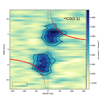
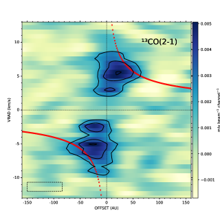
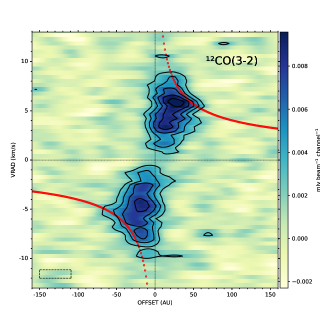
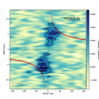
Figure 11: Top: Position-Velocity diagram of ¹²CO (2$-$1) (left) and ¹³CO (2$-$1) (right). The red dots are the maximum keplerian velocities, and the black contours levels at 3, 6, 9, 12 times the RMS (0.79 and 0.73 mJy beam^-1, respectively). Bottom: Same for ¹²CO (3$-$2) and ¹³CO (3$-$2), left and right panel respectively. The RMS for ¹²CO (3$-$2) and ¹³CO (3$-$2) are 1.11 and 1.53 mJy beam^-1.

We produced Position-velocity (PV) diagrams using Astropy and SpectralCube libraries in Python. Position-velocity slices were extracted by integrating $\sim$25 au (0.19″) above and below the midplane disk (in the direction perpendicular to the disk’s major axis). Figure 11 shows the PV diagrams for the different molecular transitions.

Similar to Matrà et al. (2017a) we compute the ratio of the PV diagrams of the different molecules/transitions (the ratios between the (3-2) and (2-1) transitions of each molecule, and the ratios between the two molecules in same transition).

For this we produced new cubes with TCLEAN, in which the angular and spectral resolution of Band 7 data are degraded in order to match the resolution of the Band 6 datasets. The PV diagrams of each molecule were combined in order to compute the different ratios in spaxels with signal higher than 4$\sigma$. Figure 12 shows the ratio between the PV diagrams of ¹²CO(3$-$2) and ¹²CO(2$-$1), and ¹³CO (3$-$2) and ¹³CO(2$-$1). Figure 13 shows the ratio between the PV diagrams of ¹²CO and ¹³CO for each transition. Figure 14 shows the resulting optical depths.

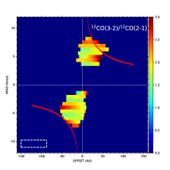
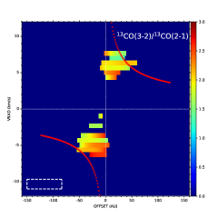
Figure 12: Ratio of the ¹²CO(3$-$2) and ¹²CO(2$-$1) P-V diagrams (left). Ratio of the ¹³CO (3$-$2) and ¹³CO (2$-$1) P-V diagrams (right). The ratios are computed in spaxels where both P-V diagrams have signal higher than 4$\sigma$.

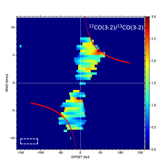
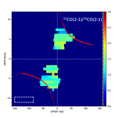
Figure 13: Position-Velocity diagram of ¹²CO(3$-$2)/¹³CO(3$-$2) (left) and ¹²CO(2$-$1)/¹³CO(2$-$1) (right). The ratios are computed in spaxels where both P-V diagrams have signal higher than 4$\sigma$.

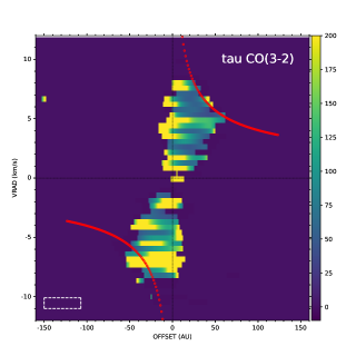
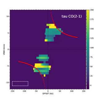
Figure 14: P-V diagram of ¹²CO optical depth from (3$-$2) (left) and CO(2$-$1) (right). The ¹²CO optical depth $\tau$ was obtained by solving $R\times(1-e^{-\tau/76})=1-e^{-\tau}$, where R is the ¹²CO/ ¹³CO line ratio.

Appendix B Channel maps and gas models.

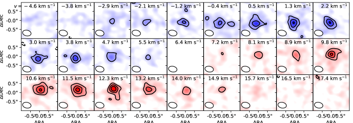
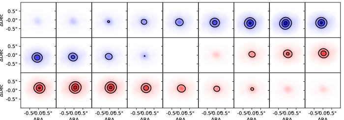
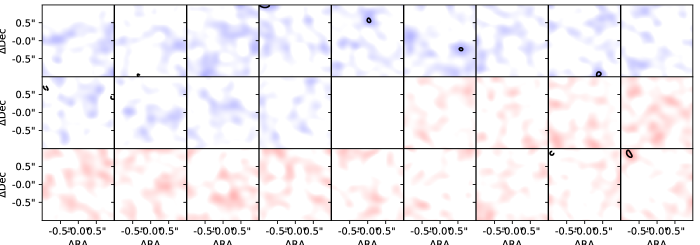
Figure 15: ¹²CO(3-2) channel maps for HD 110058, best-fit disk model (middle) and residuals (bottom). The model image is generated by using GALARIO to Fourier transform the best-fit model image onto the same baselines as the ALMA visibility data, and then imaged using a CLEAN implementation built into pdspy. The residual image is similarly made by subtracting the best-fit model visibilities from the data and then imaging. We show solid contours starting at $3\sigma$, with increments of $3\sigma$ (the RMS per channel is 1.11 mJy beam^-1). Similarly, dashed contours show emission starting at $-3\sigma$ and continuing in increments of $-3\sigma$.

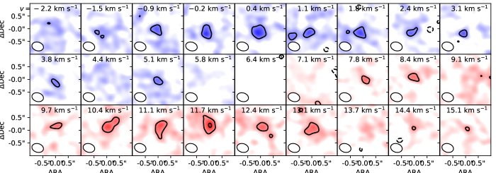
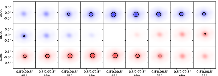
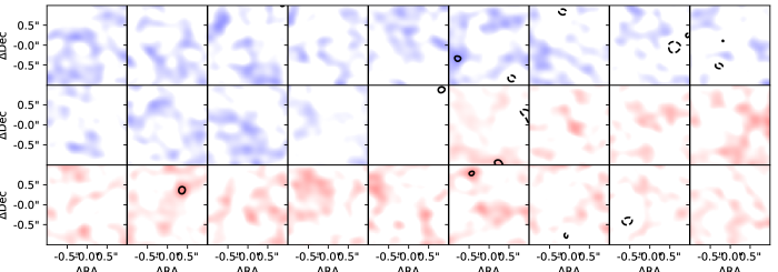
Figure 16: ¹³CO(3-2) channel maps for HD 110058, best-fit disk model (middle) and residuals (bottom). Contour levels are the same as for Figure 15. The RMS per channel is 1.53 mJy beam^-1.

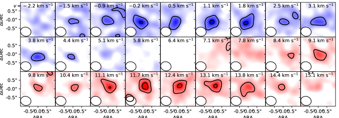
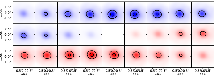
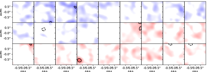
Figure 17: ¹³CO(2-1) channel maps for HD 110058, best-fit disk model (middle) and residuals (bottom). Contour levels are the same as for Figure 15. The RMS per channel is 0.73 mJy beam^-1.

References

- Astropy Collaboration et al. (2013) Astropy Collaboration, Robitaille, T. P., Tollerud, E. J., et al. 2013, A&A, 558, AA33
- Augereau et al. (2001) Augereau, J. C., Nelson, R. P., Lagrange, A. M., et al. 2001, A&A, 370, 447. doi:10.1051/0004-6361:20010199
- Brandt (2021) Brandt, T. D. 2021, ApJS, 254, 42. doi:10.3847/1538-4365/abf93c
- Brown (2001) Brown, M. E. 2001, AJ, 121, 2804. doi:10.1086/320391
- Cataldi et al. (2020) Cataldi, G., Wu, Y., Brandeker, A., et al. 2020, ApJ, 892, 99. doi:10.3847/1538-4357/ab7cc7
- Currie et al. (2014) Currie, M. J., Berry, D. S., Jenness, T., et al. 2014, Astronomical Data Analysis Software and Systems XXIII, 485, 391
- Czekala et al. (2019) Czekala, I., Chiang, E., Andrews, S. M., et al. 2019, ApJ, 883, 22
- Collings et al. (2004) Collings, M. P., Anderson, M. A., Chen, R., et al. 2004, MNRAS, 354, 1133. doi:10.1111/j.1365-2966.2004.08272.x
- Daley et al. (2019) Daley, C., Hughes, A. M., Carter, E. S., et al. 2019, ApJ, 875, 87. doi:10.3847/1538-4357/ab1074
- Dawson et al. (2011) Dawson, R. I., Murray-Clay, R. A., & Fabrycky, D. C. 2011, ApJ, 743, L17. doi:10.1088/2041-8205/743/1/L17
- Duncan & Levison (1997) Duncan M. J., Levison H. F., 1997, Sci, 276, 1670. doi:10.1126/science.276.5319.1670
- Dullemond et al. (2012) Dullemond, C. P., Juhasz, A., Pohl, A., et al. 2012, RADMC-3D: A multi-purpose radiative transfer tool, ascl:1202.015
- Esposito et al. (2020) Esposito, T. M., Kalas, P., Fitzgerald, M. P., et al. 2020, AJ, 160, 24. doi:10.3847/1538-3881/ab9199
- Foreman-Mackey et al. (2013) Foreman-Mackey, D., Hogg, D. W., Lang, D., & Goodman, J. 2013, PASP, 125, 306
- Gaia Collaboration et al. (2018) Gaia Collaboration, Brown, A. G. A., Vallenari, A., et al. 2018, A&A, 616, A1
- Goldman et al. (2018) Goldman, B., Röser, S., Schilbach, E., et al. 2018, ApJ, 868, 32. doi:10.3847/1538-4357/aae64c
- Hales et al. (2017) Hales, A. S., Barlow, M. J., Crawford, I. A., & Casassus, S. 2017, MNRAS, 466, 3582
- Hales et al. (2019) Hales, A. S., Gorti, U., Carpenter, J. M., et al. 2019, ApJ, 878, 113. doi:10.3847/1538-4357/ab211e
- Hudson (1971) Hudson, R. D. 1971, Reviews of Geophysics and Space Physics, 9, 305. doi:10.1029/RG009i002p00305
- Hughes et al. (2017) Hughes, A. M., Lieman-Sifry, J., Flaherty, K. M., et al. 2017, ApJ, 839, 86. doi:10.3847/1538-4357/aa6b04
- Hughes et al. (2018) Hughes, A. M., Duchêne, G., & Matthews, B. C. 2018, ARA&A, 56, 541
- Jewitt et al. (2017) Jewitt, D., Hui, M.-T., Mutchler, M., et al. 2017, ApJ, 847, L19. doi:10.3847/2041-8213/aa88b4
- Kasper et al. (2015) Kasper, M., Apai, D., Wagner, K., et al. 2015, ApJ, 812, L33. doi:10.1088/2041-8205/812/2/L33
- Kennedy et al. (2018) Kennedy, G. M., Marino, S., Matrà, L., et al. 2018, MNRAS, 475, 4924. doi:10.1093/mnras/sty135
- Kervella et al. (2022) Kervella, P., Arenou, F., & Thévenin, F. 2022, A&A, 657, A7. doi:10.1051/0004-6361/202142146
- Kóspál et al. (2013) Kóspál, Á., Moór, A., Juhász, A., et al. 2013, ApJ, 776, 77
- Kral et al. (2016) Kral, Q., Wyatt, M., Carswell, R. F., et al. 2016, MNRAS, 461, 845. doi:10.1093/mnras/stw1361
- Kral et al. (2017) Kral, Q., Matrà, L., Wyatt, M. C., & Kennedy, G. M. 2017, MNRAS, 469, 521
- Kral et al. (2019) Kral, Q., Marino, S., Wyatt, M. C., et al. 2019, MNRAS, 489, 3670. doi:10.1093/mnras/sty2923
- Kral et al. (2020) Kral, Q., Davoult, J., & Charnay, B. 2020, Nature Astronomy, 4, 1009. doi:10.1038/s41550-020-1205-1
- Kral et al. (2020) Kral, Q., Matrà, L., Kennedy, G. M., et al. 2020, MNRAS, 497, 2811. doi:10.1093/mnras/staa2038
- Lecavelier Des Etangs, Vidal-Madjar, & Ferlet (1998) Lecavelier Des Etangs A., Vidal-Madjar A., Ferlet R., 1998, A&A, 339, 477
- Lewis & Carver (1983) Lewis, B. R. & Carver, J. H. 1983, J. Quant. Spec. Radiat. Transf., 30, 297. doi:10.1016/0022-4073(83)90027-4
- Lieman-Sifry et al. (2016) Lieman-Sifry, J., Hughes, A. M., Carpenter, J. M., et al. 2016, ApJ, 828, 25
- Lynden-Bell & Pringle (1974) Lynden-Bell, D. & Pringle, J. E. 1974, MNRAS, 168, 603. doi:10.1093/mnras/168.3.603
- MacGregor et al. (2019) MacGregor, M. A., Weinberger, A. J., Nesvold, E. R., et al. 2019, ApJ, 877, L32. doi:10.3847/2041-8213/ab21c2
- Mannings & Barlow (1998) Mannings, V. & Barlow, M. J. 1998, ApJ, 497, 330. doi:10.1086/305432
- Marino et al. (2016) Marino, S., Matrà, L., Stark, C., et al. 2016, MNRAS, 460, 2933. doi:10.1093/mnras/stw1216
- Marino et al. (2017) Marino, S., Wyatt, M. C., Panić, O., et al. 2017, MNRAS, 465, 2595
- Marino et al. (2018) Marino, S., Carpenter, J., Wyatt, M. C., et al. 2018, MNRAS, 479, 5423. doi:10.1093/mnras/sty1790
- Marino et al. (2019) Marino, S., Yelverton, B., Booth, M., et al. 2019, MNRAS, 484, 1257. doi:10.1093/mnras/stz049
- Marino et al. (2020) Marino, S., Flock, M., Henning, T., et al. 2020, MNRAS, 492, 4409. doi:10.1093/mnras/stz3487
- Marino et al. (2020) Marino, S., Zurlo, A., Faramaz, V., et al. 2020, MNRAS, 498, 1319. doi:10.1093/mnras/staa2386
- Marino (2021) Marino, S. 2021, MNRAS, 503, 5100. doi:10.1093/mnras/stab771
- Marino et al. (2022) Marino S., Cataldi G., Jankovic M. R., Matrà L., Wyatt M. C., 2022, MNRAS.tmp. doi:10.1093/mnras/stac1756
- Matrà et al. (2017a) Matrà, L., Dent, W. R. F., Wyatt, M. C., et al. 2017, MNRAS, 464, 1415
- Matrà et al. (2017b) Matrà, L., MacGregor, M. A., Kalas, P., et al. 2017, ApJ, 842, 9
- Matrà et al. (2018) Matrà, L., Marino, S., Kennedy, G. M., et al. 2018, ApJ, 859, 72. doi:10.3847/1538-4357/aabcc4
- Matrà et al. (2019) Matrà, L., Wyatt, M. C., Wilner, D. J., et al. 2019, AJ, 157, 135. doi:10.3847/1538-3881/ab06c0
- Meshkat et al. (2015) Meshkat, T., Bailey, V. P., Su, K. Y. L., et al. 2015, ApJ, 800, 5. doi:10.1088/0004-637X/800/1/5
- McMullin et al. (2007) McMullin, J. P., Waters, B., Schiebel, D., Young, W., & Golap, K. 2007, Astronomical Data Analysis Software and Systems XVI, 376, 127
- Miotello et al. (2014) Miotello, A., Bruderer, S., & van Dishoeck, E. F. 2014, A&A, 572, A96. doi:10.1051/0004-6361/201424712
- Moór et al. (2017) Moór, A., Curé, M., Kóspál, Á., et al. 2017, ApJ, 849, 123
- Moór et al. (2019) Moór, A., Kral, Q., Ábrahám, P., et al. 2019, ApJ, 884, 108. doi:10.3847/1538-4357/ab4272
- Moór et al. (2020) Moór, A., Kóspál, Á., Ábrahám, P., et al. 2020, Origins: From the Protosun to the First Steps of Life, 345, 349. doi:10.1017/S1743921319001972
- Mouillet et al. (1997) Mouillet, D., Larwood, J. D., Papaloizou, J. C. B., et al. 1997, MNRAS, 292, 896. doi:10.1093/mnras/292.4.896
- Olofsson et al. (2022) Olofsson J., Thébault P., Kral Q., Bayo A., Boccaletti A., Godoy N., Henning T., et al., 2022, MNRAS, 513, 713. doi:10.1093/mnras/stac455
- Pan & Schlichting (2012) Pan, M. & Schlichting, H. E. 2012, ApJ, 747, 113. doi:10.1088/0004-637X/747/2/113
- Pecaut & Mamajek (2013) Pecaut, M. J. & Mamajek, E. E. 2013, ApJS, 208, 9. doi:10.1088/0067-0049/208/1/9
- Péricaud et al. (2017) Péricaud, J., Di Folco, E., Dutrey, A., et al. 2017, A&A, 600, A62. doi:10.1051/0004-6361/201629371
- Rebollido et al. (2018) Rebollido, I., Eiroa, C., Montesinos, B., et al. 2018, A&A, 614, A3
- Rosenfeld et al. (2013) Rosenfeld, K. A., Andrews, S. M., Hughes, A. M., et al. 2013, ApJ, 774, 16. doi:10.1088/0004-637X/774/1/16
- Rubin et al. (2019) Rubin, M., Bekaert, D. V., Broadley, M. W., et al. 2019, ACS Earth and Space Chemistry, 3, 1792. doi:10.1021/acsearthspacechem.9b00096
- Saffe et al. (2021) Saffe, C., Miquelarena, P., Alacoria, J., et al. 2021, A&A, 647, A49. doi:10.1051/0004-6361/202040132
- Sheehan et al. (2019) Sheehan, P. D., Wu, Y.-L., Eisner, J. A., et al. 2019, The Astrophysical Journal, 874, 136
- Takeuchi & Artymowicz (2001) Takeuchi, T. & Artymowicz, P. 2001, ApJ, 557, 990. doi:10.1086/322252
- Tazzari et al. (2017) Tazzari, M., Beaujean, F., & Testi, L. 2017, Astrophysics Source Code Library. ascl:1710.022
- Wahhaj et al. (2013) Wahhaj, Z., Liu, M. C., Nielsen, E. L., et al. 2013, ApJ, 773, 179. doi:10.1088/0004-637X/773/2/179
- Wallace et al. (1997) Wallace, P. T., Clayton, C. A., & Bly, M. J. 1997, Starlink User Note, 78
- Wilson & Rood (1994) Wilson, T. L., & Rood, R. 1994, ARA&A, 32, 191
- Wisdom (1980) Wisdom J., 1980, AJ, 85, 1122. doi:10.1086/112778
- Wyatt et al. (1999) Wyatt, M. C., Dermott, S. F., Telesco, C. M., et al. 1999, ApJ, 527, 918. doi:10.1086/308093
- Wyatt et al. (2007) Wyatt M. C., Smith R., Greaves J. S., Beichman C. A., Bryden G., Lisse C. M., 2007, ApJ, 658, 569. doi:10.1086/510999
- Wyatt (2008) Wyatt, M. C. 2008, ARA&A, 46, 339
- Wyatt et al. (2015) Wyatt, M. C., Panić, O., Kennedy, G. M., & Matrà, L. 2015, Ap&SS, 357, 103