Abstract

One key challenge for multi-task Reinforcement learning (RL) in practice is the absence of task indicators. Robust RL has been applied to deal with task ambiguity, but may result in over-conservative policies. To balance the worst-case (robustness) and average performance, we propose Group Distributionally Robust Markov Decision Process (GDR-MDP), a flexible hierarchical MDP formulation that encodes task groups via a latent mixture model. GDR-MDP identifies the optimal policy that maximizes the expected return under the worst-possible qualified belief over task groups within an ambiguity set. We rigorously show that GDR-MDP’s hierarchical structure improves distributional robustness by adding regularization to the worst possible outcomes. We then develop deep RL algorithms for GDR-MDP for both value-based and policy-based RL methods. Extensive experiments on Box2D control tasks, MuJoCo benchmarks, and Google football platforms show that our algorithms outperform classic robust training algorithms across diverse environments in terms of robustness under belief uncertainties. Demos are available on our project page (https://sites.google.com/view/gdr-rl/home).

1 Introduction

Reinforcement learning (RL) has demonstrated extraordinary capabilities in sequential decision-making, even for handling multiple tasks [1, 2, 3, 4]. With policies conditioned on accurate task-specific contexts, RL agents could perform better than ones without access to context information [5, 6]. However, one key challenge for contextual decision-making is that, in real deployments, RL agents may only have incomplete information about the task to solve. In principle, agents could adaptively infer the latent context with data collected across an episode, and prior knowledge about tasks [7, 8, 9]. However, the context estimates may be inaccurate [10, 11] due to limited interactions, poorly constructed inference models, or intentionally injected adversarial perturbations. Blindly trusting the inferred context and performing context-dependent decision-making may lead to significant performance drops or catastrophic failures in safety-critical situations. Therefore, in this work, we are motivated to study the problem of robust decision-making under the task estimate uncertainty.

Prior works about robust RL involve optimizing over the worst-case qualified elements within one uncertainty set [12, 13]. Such robust criterion assuming the worst possible outcome may lead to overly conservative policies, or even training instabilities [14, 15, 16]. For instance, an autonomous agent trained with robust methods may always assume the human driver is aggressive regardless of recent interactions and wait until the road is clear, consequently blocking the traffic. Therefore, balancing the robustness against task estimate uncertainties and the performance when conditioned on the task estimates is still an open problem. We provide one solution to address the above problem by modeling the commonly existing similarities between tasks under distributionally robust Markov Decision Process (MDP) formulations.

Each task is typically represented by a unique combination of parameters or a multi-dimensional context in multi-task RL. We argue that some parameters are more important than others in terms of affecting the environment dynamics model and thus tasks can be properly clustered into mixtures according to the more crucial parameters as in Figure 1 (a) and (b). However, existing robust MDP formulations [12] lack the capacity to model task groups, or equivalently, task subpopulations. Thus the effect of task subpopulations on the policy’s robustness is unexplored. In this paper, we show that the task subpopulations help balance the worst-case performance (robustness) and average performance under conditions (Section 5.2).

In contrast to prior work [10] that leverages point estimates of latent contexts, we take a probabilistic point of view and represent the task subpopulation estimate with a belief distribution. Holding a belief of the task subpopulation, which is the high-level latent variable, helps leverage the prior distributional information of task similarities. It also naturally copes with distributionally robust optimization by optimizing w.r.t. the worst-possible belief distribution within an ambiguity set. We consider an adaptive setting in line with system identification methods [17], where the belief is initialized as a uniform distribution and then updated during one episode. Our problem formation is related to the ambiguity modeling [18] inspired by human’s bounded rationality to approximate and handle distributions, which has been studied in behavioral economics [19, 20] yet has not been widely acknowledged in RL.

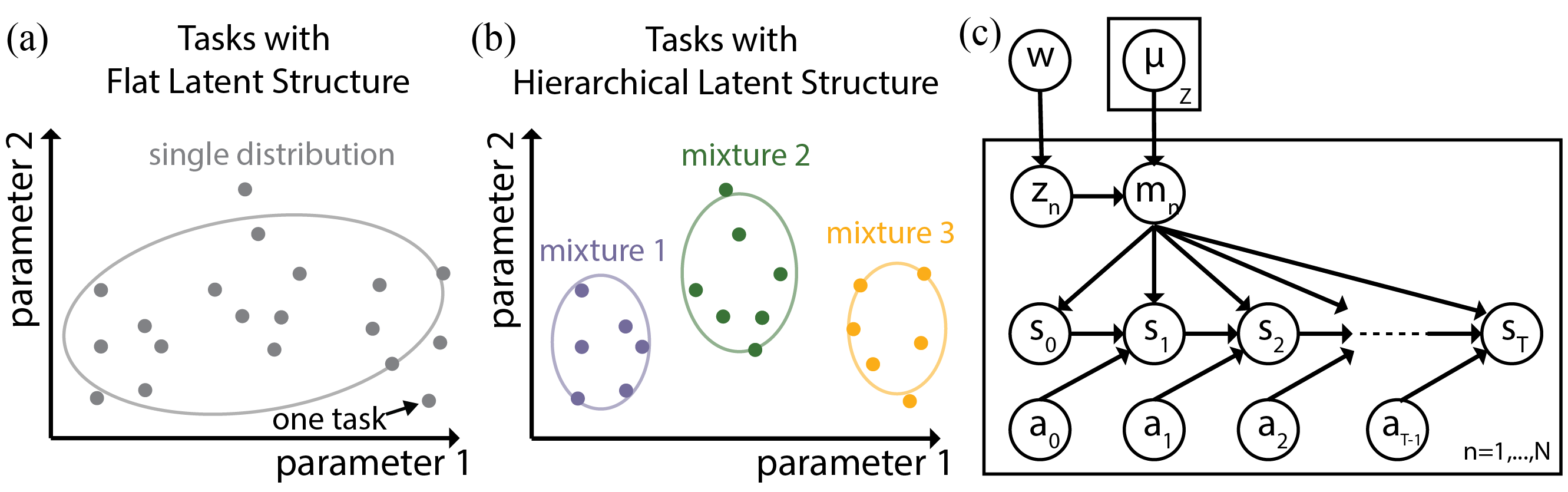
Figure 1: Illustration examples when modeling tasks with a flat latent structure that uses one distribution for all tasks as in (a), and a hierarchical latent structure that clusters tasks to different mixtures as in (b). The graphical model with a hierarchical latent structure for both GDR-MDP and HLMDP is shown in (c). At episode $n$, a mixture $z_{n}$ is first sampled from a prior distribution $w$. An MDP $m$ is then sampled according to $\mu_{z_{n}}(m)$ and controls the dynamics of the $n$’th episode.

We highlight our main contributions as follows:

1. We formulate Hierarchical-Latent MDP (HLMDP) (Section 4), which utilizes a mixture model over MDPs to encode task subpopulations. HLMDP has a high-level latent variable $z$ as the mixture, and a low-level $m$ to represent tasks (Figure 1 (c)).

2. We introduce the Group Distributionally Robust MDP (GDR-MDP) in Section 5 to handle the over-conservative problem, which formulates the robustness w.r.t. the ambiguity of the adaptive belief $b(z)$ over mixtures. GDR-MDP builds on distributionally robust optimization [21, 22] and HLMDP to leverage rich distributional information.

3. We show the convergence property of GDR-MDP in the infinite-horizon case. We find that the hierarchical latent structure helps restrict the worst-possible outcome within the ambiguity set and thus helps generate less conservative policies with higher optimal values.

4. We design robust deep RL training algorithms based on GDR-MDP by injecting perturbations to beliefs stored in the data buffer. We empirically evaluate in three environments, including robotic control tasks and google research football tasks. Our results demonstrate that our proposed algorithms outperform baselines in terms of robustness to belief noise.

2 Related Work

Robust RL and Distributionally Robust RL.

RL’s vulnerability to uncertainties has attracted large efforts to design proper robust MDP formulations accounting for uncertainties in MDP components [12, 13, 23, 24, 25, 26]. Existing robust deep RL algorithms [27, 28, 29, 30, 31, 24] are shown to generate robust policies with promising results in practice. However, it is also known that robust RL that optimizes over the worst-possible elements in the uncertainty set may generate over-conservative policies by trading average performance for robustness and may even lead to training instabilities [16]. In contrast, distributionally robust RL [32, 33, 34, 35, 36, 37, 38, 39] assumes that the distribution of uncertain components (such as transition models) is partially/indirectly observable. It builds on distributionally robust optimization [21, 22] which optimizes over the worst possible distribution within the ambiguity set. Compared with common robust methods, distributionally robust RL embeds prior probabilistic information and generates less conservative policies with carefully calibrated ambiguity sets [32]. We aim to propose distributionally robust RL formulations and training algorithms to handle task estimate uncertainties while maintaining a trade-off between robustness and performance.

One relevant work is the recently proposed distributionally robust POMDP [37] which maintains a belief over states and finds the worst possible transition model distribution within an ambiguity set. We instead hold a belief over task mixtures and find the worst possible belief distribution. [38] also maintains a belief distribution over tasks but models tasks with a flat latent structure. Moreover, [38] achieves robustness by optimizing at test-time, while we aim to design robust training algorithms to save computation during deployment.

RL with Task Estimate Uncertainty.

Inferring the latent task as well as utilizing the estimates in decision-making have been explored under the framework of Bayesian-adaptive MDPs [40, 41, 42, 43, 17]. Our work is similar to Bayesian-adaptive MDPs in terms of updating a belief distribution with Bayesian update rules, but we focus on the robustness against task estimate uncertainties at the same time. The closest work to our research is [10], which optimizes a conditional value-at-risk objective and maintains an uncertainty set centered on a context point estimate. Instead, we maintain an ambiguity set over beliefs and further consider the presence of task subpopulations. [11] also considers the uncertainties in belief estimates but with a flat latent task structure.

Multi-task RL.

Learning a suite of tasks with an RL agent has been studied under different frameworks [3, 44], such as Latent MDP [45], Multi-model MDP [5], Contextual MDP [46], Hidden Parameter MDP [47], and etc [48]. Our proposed HLMDP builds on the Latent MDP [45] which contains a finite number of MDPs, each accompanied by a weight. In contrast to Latent MDP utilizing a flat structure to model each MDP’s probability, HLMDP leverages a rich hierarchical model to cluster MDPs to a finite number of mixtures. In addition, HLMDP is a special yet important subclass of POMDP [49]. It treats the latent task mixture that the current environment belongs to as the unobservable variable. HLMDP resembles the recently proposed Hierarchical Bayesian Bandit [50] model but focuses on more complex MDP settings.

3 Preliminary

This section introduces Latent MDP and the adaptive belief setting, both serving as building blocks for our proposed HLMDP (Section 4) and GDR-MDP (Section 5).

Latent MDP.

An episodic Latent MDP [45] is specified by a tuple $({\mathcal{M}},T,{\mathcal{S}},{\mathcal{A}},\mu)$. ${\mathcal{M}}$ is a set of MDPs with cardinality $|{\mathcal{M}}|=M$. Here $T$, ${\mathcal{S}}$, and ${\mathcal{A}}$ are the shared episode length (planning horizon), state, and action space, respectively. $\mu$ is a categorical distribution over MDPs and $\sum_{m=1}^{M}\mu(m)=1$. Each MDP ${\mathcal{M}}_{m}\in{\mathcal{M}},m\in[M]$ is a tuple $(T,{\mathcal{S}},{\mathcal{A}},{\textnormal{P}}_{m},{\textnormal{R}}_{m},\nu_{m})$ where ${\textnormal{P}}_{m}$ is the transition probability, ${\textnormal{R}}_{m}$ is the reward function and $\nu_{m}$ is the initial state distribution.

Latent MDP assumes that at the beginning of each episode, one MDP from set ${\mathcal{M}}$ is sampled based on $\mu(m)$. It aims to find a policy $\pi$ that maximizes the accumulated expected return solving $\max_{\pi}\sum_{m=1}^{M}\mu(m)\mathbb{E}_{m}^{\pi}\big{[}\sum_{t=1}^{T}r_{t}\big{]}$, where $\mathbb{E}_{m}[\cdot]$ denotes $\mathbb{E}_{{\textnormal{P}}_{m},{\textnormal{R}}_{m}}[\cdot]$.

The Adaptive Belief Setting

In general, a belief distribution contains the probability of each possible MDP that the current environment belongs to. The adaptive belief setting [5] holds a belief distribution that is dynamically updated with streamingly observed interactions and prior knowledge about the MDPs. In practice, prior knowledge may be acquired by rule-based policies or data-driven learning methods. For example, it is possible to pre-train in simulated complete information scenarios or exploit unsupervised learning methods based on online collected data [51]. There also exist multiple choices for updating the belief, such as applying the Bayesian rule as in POMDPs [49] and representing beliefs with deep recurrent neural nets [52].

4 Hierarchical Latent MDP

In realistic settings, tasks share similarities, and task subpopulations are common. Although different MDP formulations are proposed to solve multi-task RL, the task relationships are in general overlooked. To fill in the gap, we first propose Hierarchical Latent MDP (HLMDP), which utilizes a hierarchical mixture model to represent distributions over MDPs. Moreover, we consider the adaptive belief setting to leverage prior information about tasks.

Definition 1 (Hierarchical Latent MDPs).

An episodic HLMDP is defined by a tuple $({\mathcal{Z}},{\mathcal{M}},T,{\mathcal{S}},{\mathcal{A}},w)$. ${\mathcal{Z}}$ denotes a set of Latent MDPs and $|{\mathcal{Z}}|=Z$. ${\mathcal{M}}$ is a set of MDPs with cardinality $|{\mathcal{M}}|=M$ shared by different Latent MDPs. $T$, ${\mathcal{S}}$, and ${\mathcal{A}}$ are the shared episode length (planning horizon), state, and action space, respectively. Each Latent MDP ${\mathcal{Z}}_{z}\in{\mathcal{Z}},z\in[Z]$ consists of a set of joint MDPs $\{{\mathcal{M}}_{m}\}_{m=1}^{M}$ and their weights $\mu_{z}$ satisfying $\sum_{m=1}^{M}\mu_{z}(m)=1$. $w$ is the categorical distribution over Latent MDPs and $\sum_{z=1}^{Z}w(z)=1$.

We provide a graphical model of HLMDP in Figure 1 (c). HLMDP assumes that at the beginning of each episode, the environment first samples a Latent MDP $z\sim w(z)$ and then samples an MDP $m\sim\mu_{z}(m)$. HLMDP encodes task similarity information via the mixture model, and thus contains richer task information than Latent MDP proposed in [45]. For instance, we could always find one Latent MDP for each HLMDP. However, there may exist infinitely many corresponding HLMDPs given one Latent MDP.

HLMDP in Adaptive Belief Setting.

When solving multi-task RL problems, the adaptive setting is shown to help generate a policy with a higher performance [5] than the non-adaptive one since it leverages prior knowledge about the transition model as well as the online collected data tailored to the unseen environment. Hence we are motivated to formulate HLMDP in the adaptive belief setting.

HLMDP maintains a belief distribution $b(z)$ over task groups to model the probability that the current environment belongs to each group $z$. At the beginning of each episode, we initialize the belief distribution with a uniform distribution $b_{0}$. We use the Bayesian rule to update beliefs based on interactions and a prior knowledge base. Note that the knowledge base are not accurate enough and may lead to inaccurate belief updates. At timestep $t$, we get the next belief estimate $b_{t+1}$ with the state estimation function $SE$:

$$SE(b_{t},s_{t})=\frac{b_{t}(j)L(j)}{\sum_{i\in[Z]}b_{t}(i)L(i)},\forall j\in[Z],$$ (1)

wher Under the adaptive belief setting, HLMDP aims to find an optimal policy $\bar{\pi}^{\star}$ within a history-dependent policy class $\Pi$, under which the discounted expected cumulative reward is maximized as in Equation 2. Following general notations in POMDPs, we denote the history at time $t$ as $h_{t}=(s_{0},a_{1},s_{1},\dots,s_{t-1},a_{t-1},s_{t})\in\mathcal{H}_{t}$ containing state-action pairs $(s,a)$. At timestep $t$, we use both the observed state $s_{t}$ and the inferred belief distribution $b_{t}(z)$ as the sufficient statistics for history $h_{t}$.

$$\bar{V}^{\star} =\max_{\pi\in\Pi}\mathbb{E}_{b_{0:T}(z)}\mathbb{E}_{\mu_{z}(m)}\mathbb{E}_{m}^{\pi}\big{[}\sum_{t=1}^{T}\gamma^{t}r_{t}\big{]},$$ (2)

where $r_{t}$ denotes the reward received at step $t$. $b_{0}(z)$ is the initial belief at timestep 0.

5 Group Distributionally Robust MDP

The belief update function in Equation 1 may not be accurate, which motivates robust decision-making under belief estimate errors. In this section, we introduce Group Distributionally Robust MDP (GDR-MDP) which models task groups and considers robustness against the belief ambiguity. We then study the convergence property of GDR-MDP in the infinite-horizon case in Section 5.1. We find that GDR-MDP’s hierarchical structure helps restrict the worst-possible value within the ambiguity set and provide the robustness guarantee in Section 5.2.

Definition 2 (General Ambiguity Sets).

Let $\Delta^{k}$ be a $k$-simplex. Considering a categorical belief distribution $b\in\Delta^{k}$, a general ambiguity set without special structures is defined as ${\mathcal{C}}_{\Delta^{k}}$ containing all possible distributions for $b$.

Definition 3 (Group Distributionally Robust MDP).

An episodic GDR-MDP is defined by a 8-tuple $({\mathcal{C}},{\mathcal{Z}},{\mathcal{M}},T,{\mathcal{S}},{\mathcal{A}},w,SE)$. ${\mathcal{C}}$ is a general belief ambiguity set. $T,{\mathcal{S}},{\mathcal{A}},{\mathcal{M}},{\mathcal{Z}},w$ are elements of an episodic HLMDP as in Definition 1. $SE:\Delta^{Z-1}\times{\mathcal{S}}\rightarrow\Delta^{Z-1}$ is the belief updating rule. GDR-MDP aims to find a policy $\pi^{\star}\in\Pi$ that obtains the following optimal value:

$$V^{\star} =\max_{\pi\in\Pi}\min_{\begin{subarray}{c}\hat{b}_{0:T}\\ \in{\mathcal{C}}_{\Delta^{Z-1}}\end{subarray}}\mathbb{E}_{\hat{b}_{0:T}(z)}\mathbb{E}_{\mu_{z}(m)}\mathbb{E}_{m}^{\pi}\big{[}\sum_{t=1}^{T}\gamma^{t}r_{t}\big{]},$$ (3)

where ${\mathcal{C}}_{\Delta^{Z-1}}$ is a general ambiguity set tailored to beliefs over Latent MDPs in set ${\mathcal{Z}}$.

GDR-MDP naturally balances robustness and performance by leveraging distributionally robust formulation and rich distributional information. In contrast to HLMDP, which maximizes expected return over nominal adaptive belief distribution (Equation 2), GDR-MDP aims to maximize the expected return under the worst-possible beliefs within an ambiguity set ${\mathcal{C}}_{\Delta^{Z-1}}$. Moreover, GDR-MDP optimizes over fewer optimization variables than when directly perturbing MDP model parameters or states. It resembles the group distributionally robust optimization problem in supervised learning [53, 54] but focuses on sequential decision-making in dynamic environments.

5.1 Convergence in Infinite-horizon Case

With general ambiguity sets (as in Definition 2), calculating the optimal policy is intractable [33, 39]. We propose a belief-wise ambiguity set that follows the b-rectangularity to facilitate solving the proposed GDR-MDP.

Assumption 1 (b-rectangularity).

We assume a belief-wise ambiguity set, $\tilde{{\mathcal{C}}}:=\bigotimes_{b\in\Delta^{Z-1}}{\mathcal{C}}_{b}$, where $\bigotimes$ represents Cartesian product. $b$ serves as the nominal distribution of the ambiguity set.

More concretely, the b-rectangularity assumption uncouples the ambiguity set related to different beliefs. When conditioned on beliefs at each timestep, the minimization loop selects the worst-case realization unrelated to other timesteps. The b-rectangularity assumption is motivated by the $s$-rectangularity first introduced in [23], which helps reduce a robust MDP formulation to an MDP formulation and get rid of the time-inconsistency problem [55]. Ambiguity sets beyond rectangularities are recently explored in [56, 57], which we leave for future works.

With b-rectangular ambiguity sets, we derive Bellman equations to solve Equation 3 with dynamic programming. Detailed proofs are in Appendix Section B.1.

Proposition 1 (Group Distributionally Robust Bellman Equation).

Define the distributionally robust value of an arbitrary policy $\pi$ as follows where $b_{t+1}=SE(b_{t},s_{t})$.

$$V_{t}^{\pi}(b_{t},s_{t})\!=\!\min_{\begin{subarray}{c}\hat{b}_{t:T}\in\\ {\mathcal{C}}_{b_{t:T}}\end{subarray}}\mathbb{E}_{\hat{b}_{t:T}(z)}\mathbb{E}_{\mu_{z}(m)}\mathbb{E}_{m}^{\pi_{t:T}}\!\big{[}\sum_{n=t}^{T}\gamma^{n-t}r_{n}|b_{t},s_{t}\big{]}.$$

The Group Distirbutionally Robust Bellman expectation equation is

$$V_{t}^{\pi}(b_{t},s_{t}) =\min_{\hat{b}_{t}\in{\mathcal{C}}_{b_{t}}}\mathbb{E}_{\hat{b}_{t}(z)}\mathbb{E}_{\mu_{z}(m)}\mathbb{E}^{\pi_{t}}\Big{[}\mathbb{E}_{{\textnormal{R}}_{m}}[r_{t}]+$$

$$\gamma\sum_{s_{t+1}}{\textnormal{P}}_{m}(s_{t+1}|s_{t},a_{t})V^{\pi}_{t+1}(b_{t+1},s_{t+1})\Big{]}.$$ (4)

Lemma 1 (Contraction Mapping).

Let $\mathcal{V}$ be a set of real-valued bounded functions on $\Delta^{Z-1}\times\mathcal{S}$. $\mathcal{L}V(b,s):\mathcal{V}\rightarrow\mathcal{V}$ refers to the Bellman operator defined as

$$\mathcal{L}V(b,s) =\max_{\pi\in\Pi}\min_{\hat{b}\in{\mathcal{C}}_{b}}\mathbb{E}_{\hat{b}(z)}\mathbb{E}_{\mu_{z}(m)}\mathbb{E}^{\pi}\Big{[}\mathbb{E}_{{\textnormal{R}}_{m}}[r]+$$

$$\gamma\sum_{s^{\prime}}{\textnormal{P}}_{m}(s^{\prime}|s,a)V^{\pi}(SE(b,s),s)\Big{]}.$$ (5)

$\mathcal{L}V(b,s)$ is a $\gamma$-contraction operator on the complete metric space $(\mathcal{V},\|\cdot\|_{\infty})$. That is, given $\forall\ U,V\in\mathcal{V}$, $\|\mathcal{L}U-\mathcal{L}V\|_{\infty}\leq\gamma\|U-V\|_{\infty}$.

Theorem 1 (Convergence in Infinite-horizon Case).

Define $V_{\infty}(b,s)$ as the infinite horizon value function. For all $b\in\mathcal{B}$ and $s\in\mathcal{S}$, we have $V_{\infty}(b,s)$ is the unique solution to $\mathcal{L}V_{\infty}(b,s)=V_{\infty}(b,s)$, and $\lim_{t\rightarrow\infty}\mathcal{L}V_{t}(b,s)=\mathcal{L}V_{\infty}(b,s)$ uniformly in $\|\cdot\|_{\infty}$.

By repeatedly applying the contraction operator in Lemma 1, the value function will converge to a unique fixed point, which corresponds to the optimal value based on Banach fixed point theorem [58].

5.2 Robustness Guarantee of GDR-MDP

This section shows how GDR-MDP’s hierarchical task structure and the distributionally robust formulation help balance performance and robustness. We compare the optimal value of GDR-MDP denoted as $V_{GDR}(\pi^{\star}_{GDR})$, with three different robust formulations. Group Robust MDP is a robust version of GDR-MDP with its optimal value denoted as $V_{GR}(\pi^{\star}_{GR})$. Distributionally Robust MDP holds a belief over MDPs without the hierarchical task structure whose optimal value denoted as $V_{DR}(\pi^{\star}_{DR})$. Robust MDP is a robust version of Distributionally Robust MDP, denoted as $V_{R}(\pi^{\star}_{R})$. $\pi^{\star}_{\cdot}$ denote optimal policies under different formulations. We achieve the comparison by studying how maintaining beliefs over mixtures affects the worst-possible outcome of the inner minimization problem and the resulting RL policy.

We study the worst-possible value via the relationships between ambiguity sets projected to the space of beliefs over MDPs. We first define a discrepancy-based ambiguity set that is widely used in existing DRO formulations [59, 60, 61].

Definition 4 (Ambiguity set with total variance distance).

Consider a discrepancy-based ambiguity set defined based on total variance distance. Formally, the ambiguity set is

$${\mathcal{C}}_{\nu_{{\mathcal{X}}},d_{TV},\xi}(X)=\{\nu^{\prime}(X):\sup_{X\in{\mathcal{X}}}|\nu^{\prime}(X)-\nu_{{\mathcal{X}}}(X)|\leq\xi\},$$

where $X\in{\mathcal{X}}$ is the support, $\nu_{{\mathcal{X}}}$ is the nominal distribution over ${\mathcal{X}}$ and $\xi$ is the ambiguity set’s size.

To achieve a reasonable comparison, we control the adversary’s budget $\xi$ the same when perturbing the belief over task groups $z$ and tasks $m$, which correspond to different model misspecification forms when there is a hierarchical latent structure about tasks.

Theorem 2 (Values of different robust formulations).

Let $U_{m}(\pi)=\mathbb{E}_{m}^{\pi}\big{[}\sum_{t=1}^{T}\gamma^{t}r_{t}\big{]}$. Let ${\mathcal{C}}_{b(m),d_{TV},\xi}(m)$ and ${\mathcal{C}}_{b(z),d_{TV},\xi}(z)$ denote the ambiguity sets for beliefs over tasks $m$ and groups $z$, respectively. $b(m)$ and $b(z)$ satisfy $b(m)=\sum_{{\mathcal{Z}}}\mu_{z}(m)b(z)$ and are the nominal distributions. For any history-dependent policy $\pi\in\Pi$, its value function under different robust formulations are:

$$V_{GDR}(\pi) =\min_{\hat{b}(z)\in{\mathcal{C}}_{b(z),d_{TV},\xi}(z)}\mathbb{E}_{\hat{b}(z)}\mathbb{E}_{\mu_{z}(m)}[U_{m}(\pi)],$$

$$V_{GR}(\pi) =\min_{z\in[Z]}\mathbb{E}_{\mu_{z}(m)}[U_{m}(\pi)],$$

$$V_{DR}(\pi) =\min_{\hat{b}(m)\in{\mathcal{C}}_{b(m),d_{TV},\xi}(m)}\mathbb{E}_{\hat{b}(m)}[U_{m}(\pi)],$$

$$V_{R}(\pi) =\min_{m\in[M]}[U_{m}(\pi)].$$

We have the following inequalities hold: $V_{GDR}(\pi)\geq V_{GR}(\pi)\geq V_{R}(\pi)$ and $V_{GDR}(\pi)\geq V_{DR}(\pi)$.

Theorem 2 shows that with a nontrivial ambiguity set, the distributionally robust formulation in GDR-MDP helps regularize the worst-possible value when compared with robust ones, including the group robust (GR) and task robust (R) formulations. It also shows that GDR-MDP’s hierarchical structure further helps restrict the effect of the adversary, resulting in higher values than the distributionally robust formulation with a flat latent structure (DR). To get Theorem 2, we first find that when projecting the $\xi$-ambiguity set for $b(z)$ to the space of $b(m)$, the resulting ambiguity set is a subset of the $\xi$-ambiguity set for $b(m)$. Proofs are detailed in Appendix Section B.2. Our setting is different from [62] which states that DRO is a generalization of point-wise attacks. The key difference is that when the adversary perturbs $b(m)$, we omit the expectation over the mixtures under $b(z)$.

Theorem 3 (Optimal values of different robust formulations).

Let $\pi_{\cdot}^{\star}$ denote the converged optimal policy for different robust formulations, we have $V_{GDR}(\pi_{GDR}^{\star})\geq V_{GR}(\pi_{GR}^{\star})\geq V_{R}(\pi_{R}^{\star})$ and $V_{GDR}(\pi_{GDR}^{\star})\geq V_{DR}(\pi_{DR}^{\star})$.

Based on Theorem 2, we can compare the optimal values for different robust formulations. Theorem 3 shows that imposing ambiguity set on beliefs over mixtures helps generate less conservative policies with higher optimal values at convergence compared with other robust formulations.

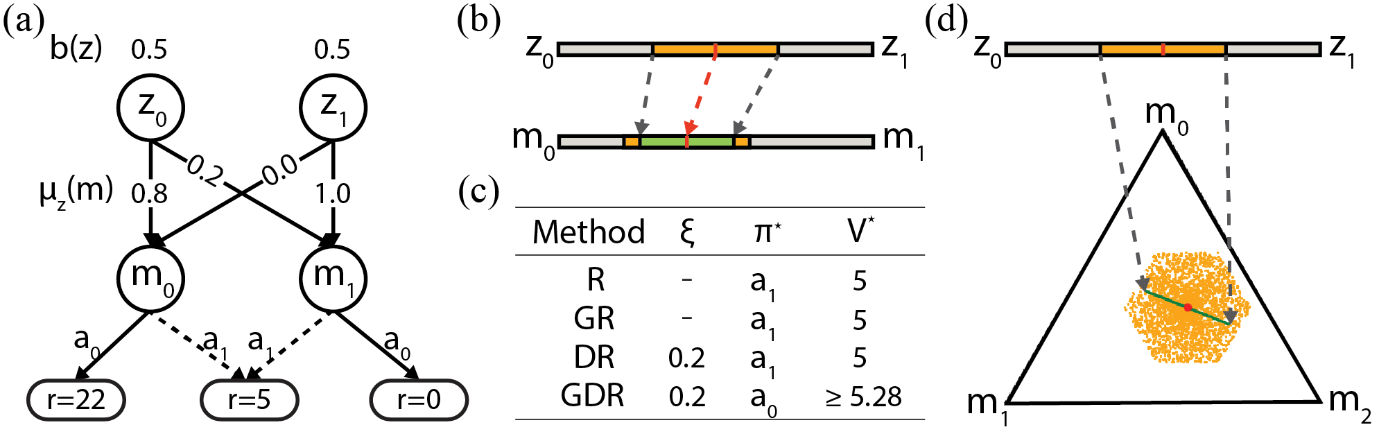
Figure 2: Hierarchical Latent Bandit examples. (a), (b) and (c) show the graphical model, the relationship between ambiguity sets, and different robust formulations’ optimal values for an example with two groups and two unique tasks. (d) shows the relationship between ambiguity sets for an example with two groups and three unique tasks.

Illustration Examples in Figure 2. We provide two hierarchical latent bandit examples in Figure 2. The first example shown in Figure 2 (a) has two latent groups with different weights over two unique MDPs. (b) shows the ambiguity sets of the example in (a). The orange sets denote the $\xi$-ambiguity sets for the beliefs over mixtures and MDPs. The green set denotes the ambiguity set projected from the $\xi$-ambiguity set for belief distributions over mixtures. We show that the mapped set is a subset of the original $\xi$-ambiguity set for the MDP belief distributions. (c) shows the optimal policy and value of different robust formulations for the example in (a). Our proposed GDR has the potential to get a less conservative policy with higher returns than other robust baselines. (d) follows the same notations in (b) but corresponds to an example with three possible MDPs. (b) and (d) together shows that the hierarchical structure helps regularize the adversary’s strength. The detailed procedure for getting the optimal policies is shown in Appendix A.

6 Algorithms

To solve the proposed GDR-MDP, we propose novel robust deep RL algorithms (summarized in Algorithm 2 and Algorithm 3 in appendix), including GDR-DQN based on Deep Q learning [1], GDR-SAC based on soft actor-critic [63], and GDR-PPO based on PPO [64]. We learn robust policies that take the inferred belief distribution over mixtures $b(z)$ and the state $s$ as input. We implement GDR-DQN and GDR-SAC with Tianshou [65] and GDR-PPO with stable-baselines3 [66]. Details are in Appendix Section D.

Input: Mixing weights $w(z)$ and $\mu_{z}(m)$, episode index $n$, episode length $T$, belief update function $SE$, rollout policy $\pi_{\theta}(b(z),s)$, exploration $\epsilon$

Initialize episodic history $h=\{\}$ ;

Sample mixture $z_{n}\sim w(z)$ ;

Sample MDP $m_{n}\sim\mu_{z_{n}}(m)$ ;

Initialize belief $b_{0}(z)$ as a uniform distribution ;

for $t=0$ to $T$ do

       Sample action $a_{t}$ with the $\epsilon$-greedy method and rollout in MDP $m$;

       $b_{t+1}(z)=SE(b_{t}(z),s_{t+1})$ ;

       Append the most recent data pair $d=\{(b_{t},s_{t}),a_{t},r_{t},(b_{t+1},s_{t+1})\}$ to $h$ ;

Return: history $h$, episode return

Algorithm 1 GDR-MDP Trajectory Rollout

GDR-DQN and GDR-SAC.

We update the Q-net in GDR-DQN and the critic net in GDR-SAC toward TD targets with perturbed beliefs. We follow Definition 4 to construct the ambiguity set ${\mathcal{C}}_{b^{\prime}(z),d_{TV},\xi}$ which centers at the originally inferred $b^{\prime}(z)$ and satisfies the b-rectangularity assumption stated in Assumption 1. At each training step, we sample a batch data $\{d=(b(z),s,a,r,b^{\prime}(z),s^{\prime},a^{\prime},r^{\prime})\}^{N}$ from the replay buffer ${\mathcal{D}}$ to estimate the perturbed TD target.

We update Q-functions with gradient descents. For both GDR-DQN and GDR-SAC, we have loss as

$${\mathcal{L}}_{Q_{\theta}}=\sum_{\begin{subarray}{c}d\end{subarray}}\Big{(} r+\min_{\begin{subarray}{c}p(z)\in\\ {\mathcal{C}}_{b^{\prime}(z),d_{TV},\xi}\end{subarray}}\sum_{a\in{\mathcal{A}}}Q_{\theta}(p(z),s^{\prime},a)$$

$$-\sum_{a\in{\mathcal{A}}}Q_{\theta}(b(z),s,a)\Big{)}^{2}.$$

GDR-PPO.

GDR-PPO conducts robust training by decreasing the advantages of trajectories that are vulnerable to belief noises. More concretely, given a trajectory $d$, its advantage for $(b_{t},s_{t})$ is calculated as follows.

$$\hat{A}(b_{t},s_{t}) =\sum_{t^{\prime}=t}^{T-1}r_{t}-R_{drop}-V_{\theta}(b_{t},s_{t}),\text{ where}$$

$$R_{drop} =V(b_{t},s_{t})-\min_{\begin{subarray}{c}p(z)\in{\mathcal{C}}_{b_{t}(z),d_{TV},\xi}\end{subarray}}V_{\theta}(p(z),s_{t}).$$

We measure the performance drop $R_{drop}$ under worst-possible beliefs within the ambiguity set.

Worst-possible Beliefs.

To obtain the worst case distribution $b^{adv}\in{\mathcal{C}}_{b^{\prime}(z),d_{TV},\xi}$, we iteratively apply a stochastic variant of fast gradient sign method (FGSM) [67] to make sure that the perturbed discrete distribution satisfies $\sum_{z}p(z)=1$. For each attack to the belief distribution, we randomly sample an index $i\in Z$, and apply the attack to each element in $p(z)$ as follows $p(z)_{j}=p(z)_{j}+\alpha_{b}\cdot\operatorname{sign}(\nabla_{p(z)_{j}}V(p(z),s^{\prime})),\forall j\not=i$ and $p(z)_{i}=p(z)_{i}-\sum_{j\not=i}p(z)_{j}$. $\alpha_{b}$ is the perturbation step size. To stabilize robust training, we pretrain for a small amount of episodes with exact one-hot beliefs to ensure that the value function could approximate the actual state value to some extent. To achieve a certain level of robustness over noisy inferred belief $b(z)$, we fix the ambiguity set size along with robust training, which is analogous to the adversary budget and the robustness level [36].

Figure 3: The training performance of GDR and baselines. Each curve is averaged over 5 runs and shaded areas represent standard errors. Our results show that GDR has better training stability than DR by implicitly regularizing the adversary’s strength with the hierarchical structure.

Input: Q-net $Q_{\theta}(b(z),s,a)$, ambiguity set ${\mathcal{C}}_{\cdot,d_{TV},\xi}$, training episodes $N$,

Initialize data buffer ${\mathcal{D}}$ ;

for $n=0$ to $N$ do

       Rollout one episode with Algorithm 1 and append data pairs to ${\mathcal{D}}$ ;

       if Update Q-net parameters then

             Sample batch data from ${\mathcal{D}}$ ;

             for Each $d_{i}$ in the batch do

                   Get $b^{adv}\in{\mathcal{C}}_{b^{\prime}(z),d_{TV},\xi}$ with modified FGSM;

                  

            Update Q-net $\theta\leftarrow\theta-\alpha_{\theta}\nabla_{\theta}{\mathcal{L}}_{Q_{\theta}}$;

            

Return: Q-net $Q_{\theta}$

Algorithm 2 Group Distributionally Robust Training for GDR-DQN and GDR-SAC

7 Experiments

We conduct experiments to empirically study (a) the effect of GDR-MDP’s hierarchical structure on the robust training stability and (b) policy’s robustness to belief estimate error.

7.1 Environments

We evaluate GDR-DQN in Lunarlander [68], GDR-SAC in Halfcheetah [69], and GDR-PPO in Google Research Football [70]. Table 1 shows a summary of environment setups. More details are in Appendix Section C. To initialize each episode, we first sample a group $z\sim w(z)$, and then a task $m\sim\mu_{z}(m)$ for the episode. Note that both $z$ and $m$ are unknown to the agent.

Google Research Football (GRF).

This domain presents additional challenges due to its AI randomness, large state-action spaces, and sparse rewards. The RL agent will control one active player on the attacking team at each step and can pass to switch control. The non-active players will be controlled by built-in AI. The dynamics of our designed 3 vs. 2 tasks are determined by the player types including central midfield (CM) and centre back (CB), and player capability levels. The built-in CM player tends to go into the penalty area when attacking and guard the player on the wing (physically left or right) when defending, while the CB player tends to guard the player in the middle when defending, and not directly go into the penalty area when attacking. Different patterns of policies are required to solve the tasks from different groups.

Box2D Control Task: LunarLander.

The Lunarlander’s dynamics are controlled by the engine mode and engine power. In the flipped mode, the action turning on the left (or right) engine in normal mode will turn on the right (or left) engine instead.

Mujoco Control Task: HalfCheetah.

In HalfCheetah, each task’s dynamics are controlled by both the torso mass and the failure joint, to which we cannot apply action. Our setting is similar to the implementation in [10] but with a fixed failure joint within each episode.

7.2 Baselines

Table 1: Environment setups. Both parameters affect the environment dynamics. In GRF, the strongest player has a capability level of 1.0. Our tasks are more challenging than the original 3 vs. 2 task in GRF (1.0 vs. 0.6) in terms of the capability level. For notation simplicity, let $\mathbf{1}^{k}$ be a k-dimensional vectored filled with 1, and $E(k)=\frac{1}{k}\mathbf{1}^{k}$. $E_{i}(k)$ shows the $i$-th matrix block on the diagonal.

Environment	GRF (3 vs. 2)	LunarLander	HalfCheetah
Parameter 1	Player Type	Engine Mode	Failure Joint
(Mixture)	{CM vs. CB, CB vs. CM}	{Normal, Flipped}	{0,1,2,3,4,5}
Parameter 2	Player Capability Level	Engine Power	Torso Mass
	{0.9 vs. 0.6, 1.0 vs. 0.7}	{3.0, 6.0}	{0.9, 1.0, 1.1}
# Mixtures	2	2	6
$w$	[0.5, 0.5]	[0.5, 0.5]	$\frac{1}{6}\mathbf{1}^{6}$
# MDPs	4	4	18
$\mu_{z}(m)$	$\begin{bmatrix}\frac{1}{2}\mathbf{1}^{2}&\mathbf{0}\\ \mathbf{0}&\frac{1}{2}\mathbf{1}^{2}\end{bmatrix}$	$\begin{bmatrix}\frac{1}{2}\mathbf{1}^{2}&\mathbf{0}\\ \mathbf{0}&\frac{1}{2}\mathbf{1}^{2}\end{bmatrix}$	$\begin{bmatrix}E_{0}(6)&\mathbf{0}&\mathbf{0}\\ \mathbf{0}&\cdots&\mathbf{0}\\ \mathbf{0}&\mathbf{0}&E_{5}(6)\\ \end{bmatrix}$

We compare our Group Distributionlly Robust training methods (GDR) with five baselines. In G-Exact, the RL agent is trained with the exact mixture information encoded in a one-hot vector. The agent in DR maintains a belief distribution $b(m)$ and utilizes distributionally robust training over $b(m)$. It uses the same belief updating rule as in GDR to update $b(z)$ at each timestep but projects $b(z)$ to $b(m)$ with $\mu_{z}(m)$. DR utilizes no mixture information and helps ablate the effect of the hierarchical latent structure. The agent in No-Belief has no access to the context information and generates action only based on state $s$. The No-Belief baseline helps show the importance of the adaptive belief setting. In G-Belief, the agent maintains belief $b(z)$ and is trained towards a nominal TD target. Compared with GDR, G-Belief helps reveal the effect of distributionally robust training. The State-R agent takes both the inferred belief $b(z)$ and state $s$ as input. It updates towards a TD target with perturbed states along with training. For baselines with belief modules, we utilize the Bayesian update rule in Equation 1 and leave the detailed likelihood calculation in Appendix Section D.

8 Results and Discussion

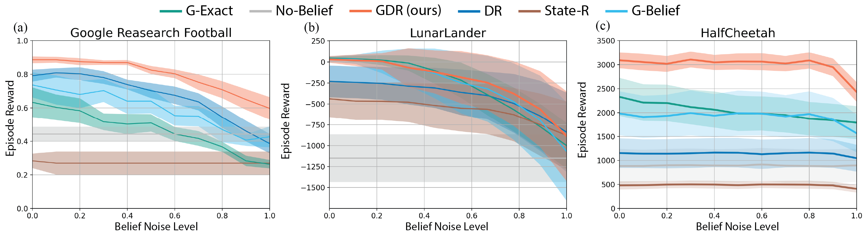
Figure 4: Robustness evaluations when facing belief inference errors. Each plot is averaged over 5 runs and shaded areas represent standard errors. GDR preserves higher robustness to belief inference errors compared with baselines.

8.1 Influence of the GDR-MDP’s Hierarchical Structure on Robust Training

We study the effect of the hierarchical structure on the adversary’s strength based on training performances in Figure 3. We show the importance of mixture information since the No-Belief baseline consistently underperforms G-Exact during training in all three environments. Lunarlander and HalfCheetah have a return much lower than G-Exact since the kinematic observation fed into the neural net does not reveal any mixture information. In GRF, the No-Belief baseline underperforms G-Exact since it could not effectively learn distinct strategies with regard to different types of players as teammates and opponents, while G-Exact could learn group-specific policies.

When compared with other robust training baselines including DR and State-R, GDR achieves a higher average return at convergence in all environments as in Figure 3. In LunarLander and HalfCheetah, DR which maintains a belief $b(m)$ over MDPs induces significant training instability, instead of learning a meaningful conservative policy. In GRF, DR has a worse asymptotic performance than GDR. Those observations empirically validate our theoretical result (Section 5.2) in the regime of deep RL, which is that, with the same ambiguity set size, perturbing $b(m)$ omitting mixture information will lead to larger value perturbations than perturbing $b(z)$ over mixtures. The State-R baseline leads to more considerable training instability than DR and fails to learn in all three environments.

We compare GDR with non-robust training baselines, including G-Exact and G-belief to study the importance of robust training. In LunarLander, GDR has comparable training performance with G-Exact and G-Belief. In GRF, GDR has slightly worse asymptotic performance than G-Exact and better performance than G-Belief. These observations show that GDR successfully extracts task-specific information stored in the noisy beliefs and conditions on the beliefs for action generation. In HalfCheetah, GDR performs better than G-Exact. Although GDR leads to an immediate performance drop after pretraining (100000 steps), the robust training in GDR converges to higher performance. We conjecture that this is due to the perturbed belief helping the algorithm get out of local optima.

8.2 Robustness to Belief Inference Errors

We test the robustness against belief noise of the best policies obtained with GDR and baselines along with training. The results are shown in Figure 4. We define the belief noise level as the inaccuracy of the likelihood when updating belief with the Bayesian rule. During robustness evaluation, G-Exact generate actions conditioned on the same noisy beliefs as GDR and G-Belief.

In GRF and HalfCheetah, GDR is consistently more robust to belief noise than robust and nominal training baselines. In LunarLander, the mean reward of GDR is better than G-Exact when there is a high belief noise level and is better than DR when a low belief noise level. The large variances in LunarLander are due to the large penalty when crashes which are further exaggerated by the fixed episode length. Although GDR has its performance decreasing along with the increase of the belief noise level, its performance is still an upper bound of DR and G-Exact’s performances. These observations show that GDR successfully balances the information between belief distributions and states, and is more robust to belief inference errors.

G-Exact is prone to injected belief noise since it heavily relies on accurate mixture information to achieve high performance. G-Belief does not show significant robustness improvement over G-Exact. It shows that the group distributionally robust training procedure instead of the belief randomness along training helps improve the robustness.

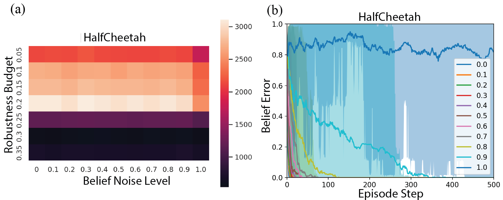
Figure 5: Ablation studies in HalfCheetah.

8.3 Ablation Study

We perform empirical sensitivity analysis to reveal the effect of uncertainty set size on GDR’s policy robustness in HalfCheetah. Figure 5 (a) shows that gradually increasing the ambiguity set size up to 0.2 helps improve the robustness. The ambiguity set whose size is greater or equal to 0.25, easily leads to training instability and thus decreases the robustness. In contrast, even with an ambiguity set of size 0.05 and pretraining for 300000 steps, DR without the mixture information still causes unstable training (see Appendix Section E). Figure 5 (b) provides the average belief errors at each time step corresponding to different belief noise levels. Figure 5 (b) and Figure 4 show that GDR only shows significant performance drops when the belief error is nonzero for a large portion of steps.

9 Conclusion

This paper considers robustness against task estimate uncertainties. We propose the GDR-MDP formulation that can leverage rich distribution information, including adaptive beliefs and prior knowledge about task groups. To the best of our knowledge, GDR-MDP is the first distributionally robust MDP formulation that models ambiguity over belief estimates in an adaptive setting. We theoretically show that GDR-MDP’s hierarchical latent structure helps enhance its distributional robustness compared with a flat task structure. We also empirically show that our proposed group distributionally robust training methods generate more robust policies than baselines when facing belief inference errors in realistic scenarios. We hope this work will inspire future research on how diverse domain knowledge affects robustness and generalization. One exciting future direction is to scale the group distributionally robust training to high-dimensional and continuous latent task distributions for diverse decision-making applications.

Appendix A Toy Example: Hierarchical Latent Bandit

In this section, we show the process of getting the optimal policies for different robust formulations in the Hierarchical Latent Bandit problem as illustrated in Figure 2 (a).

The agent has two possible actions, $a_{0}$ and $a_{1}$. There are two possible mixtures/groups denoted as $z$, and two possible MDPs denoted as $m$. Given the mixture, we have the conditional probability for each MDP as $\mu(m=0|z=0)=0.8$, $\mu(m=1|z=0)=0.2$, $\mu(m=0|z=1)=0.0$, $\mu(m=1|z=1)=1.0$. We assume the same type of ambiguity set measured by the total variance distance as in the analysis. Let the current belief over groups be $b(z)=[0.5,0.5]$ and the ambiguity set size be $\xi=0.2$.

We compare the optimal policies of four robust formulations, including

• our proposed GDR-MDP (shorthanded as GDR) that utilizes both the hierarchical structure and distributionally robust formulation, and optimizes over the worst-possible beliefs over groups,

• group robust MDP (GR), which optimizes over the worst-possible groups,

• distributionally robust MDP (DR), which holds a belief over MDPs without the hierarchical task structure and optimizes over the worst-possible belief distribution,

• robust MDP (R), which is a robust version of distributionally robust MDP and optimizes over the worst-possible MDP.

Optimal policy for R.

R desires robustness over the worst possible MDPs. We can see that the worst possible MDP is $m_{1}$ since the reward when choosing $a_{0}$ or $a_{1}$ in $m_{1}$ is consistently smaller than the rewards when in $m_{0}$. Since the optimal policy for $m_{1}$ is selecting $a_{1}$, the optimal policy for R is $a_{1}$.

Optimal policy for GR.

GR desires robustness over the worst-possible mixtures. The value for selecting $a_{0}$ under mixture $z_{0}$ is $V(a_{0}|z_{0})=22*0.8=17.6$. Similarly, $V(a_{1}|z_{0})=5$, $V(a_{0}|z_{1})=0$ and $V(a_{1}|z_{1})=5$. Assume the agent has a stochastic policy, $\pi(p)=[p,1-p]$, The value of the policy under mixture $z_{0}$ is $V(\pi(p),z_{0})=0.8*(22p+5*(1-p))+0.2*(0*p+5*(1-p))=12.6p+5$. The value of the policy under mixture $z_{1}$ is $V(\pi(p),z_{1})=0.5*(5p+0.0*(1-p))+0.5*(5p+0*(1-p))=5p$. Since $V(\pi(p),z_{1})<V(\pi(p),z_{0}),\forall p\in[0,1]$. The worst possible mixture is thus $z_{1}$ and the optimal policy for GR is $a_{1}$.

Optimal policy for DR.

DR desires robustness over the worst possible belief distribution over MDPs. The nominal $m$-level belief distribution is $b(m)=[0.4,0.6]$, which is mapped from current $z$-level belief $b(z)=[0.5,0.5]$. Considering that there always exists one deterministic policy $\pi$ as the optimal policy for each belief distribution $b^{\prime}(m)$, we directly analyze the value of the two actions with perturbed belief $\hat{b}(m)$. When the deterministic policy puts all mass on action $a_{1}$, perturbing belief doesn’t affect the resulting value estimates since each $m$ has the same reward 5 when selecting $a_{1}$. Therefore the value of $a_{1}$ is always 5. When the deterministic policy puts all mass on action $a_{0}$, the worst possible belief decreases the weight of $m_{0}$ by $\xi$, which is the maximum attack the adversary can apply. In this worst case, the value estimates of $a_{1}$ is $\hat{V}=(0.4-\xi)*22=4.4<5$. Therefore the optimal policy is $a_{1}$.

Similar results can be derived with the value function. Formally, given $\epsilon\in[-\xi,\xi]=[-0.2,0.2]$, $\pi(a_{0})=p,\pi(a_{1})=1-p$, we want to solve the following optimization problem

$$\max_{p}\min_{\epsilon}V(\pi(p),{\mathcal{C}}_{b(m),\xi}) =\max_{p}\min_{\epsilon}(0.4-\epsilon)[22p+5(1-p)]+(0.6+\epsilon)[0p+5(1-p)]$$

$$=\max_{p}\min_{\epsilon}-22p\epsilon+3.8p+5$$

Since $\frac{\partial}{\partial\epsilon}V(\pi(p),{\mathcal{C}}_{b(m),\xi})=-22p,p\in[0,1]$, we have $\operatorname*{arg\,min}_{\epsilon}V(\pi(p),{\mathcal{C}}_{b(m),\xi})=0.2$.

$$\max_{p}\min_{\epsilon}V(\pi(p),{\mathcal{C}}_{b(m),\xi}) =\max_{p}-0.6p+5$$

Therefore when $p=0$, the value is maximized. It shows that the optimal policy is $a_{1}$.

Optimal policy for GDR.

GDR instead desires robustness over the worst possible belief distribution over contexts. Similar to the analysis for DR, the value estimate of $a_{1}$, $\hat{V}(a_{1})$, is always equal to 5 regardless of the perturbed $\hat{b}(z)$. Now we need to investigate the value when selecting deterministic policy as $a_{0}$. The weight on $z_{0}$ in the perturbed belief lies in range $\hat{b}(z_{0})\in[0.5-\xi,0.5+\xi]=[0.3,0.7]$. The value estimate for $a_{0}$ is thus $\hat{V}(a_{0})=\hat{b}(z_{0})*0.8*22=17.6\hat{b}(z_{0})\in[5.28,12.32]$. Since the lower bound is larger than the value of $\hat{V}(a_{1})=5$, the optimal policy for GDR is $a_{0}$.

Similarly, we can also write out the value function and the optimization problem.

$$\max_{p}\min_{\epsilon}V(\pi(p),{\mathcal{C}}_{b(z),\xi})$$

$$= \max_{p}\min_{\epsilon}(0.5-\epsilon)[0.8*(22p+5(1-p))+0.2*(0p+5(1-p))]+(0.5+\epsilon)[0p+5(1-p)]$$

$$= \max_{p}\min_{\epsilon}-17.6p\epsilon+3.8p+5$$

Since $\frac{\partial}{\partial\epsilon}V(\pi(p),{\mathcal{C}}_{b(z),\xi})=-17.6p,p\in[0,1]$, we have $\operatorname*{arg\,min}_{\epsilon}V(\pi(p),{\mathcal{C}}_{b(z),\xi})=0.2$.

$$\max_{p}\min_{\epsilon}V(\pi(p),{\mathcal{C}}_{b(z),\xi}) =\max_{p}0.28p+5$$

Therefore when $p=1$, the value is maximized. It shows that the optimal policy is $a_{0}$.

To sum up, the Hierarchical Latent Bandit example shows that our proposed GDR-MDP has the potential to find a less conservative policy compared with other robust formulations.

Appendix B Proofs

B.1 Proofs for Section 5.1: Convergence of GDR-MDP in Infinite-horizon Case

This section proves the convergence of GDR-MDP in the infinite-horizon case. We first prove the Bellman expectation equation and Bellman optimality equation in Section B.1.1. We then show the contraction operator build on the Bellman optimality equation is a contraction operator in Section B.1.2. Finally, we show the convergence of GDR-MDP in Section B.1.3.

B.1.1 Proofs for Proposition 1

We provide the proof for the Bellman expectation equation as follows. Starting from the definition of $V_{t}^{\pi}(b_{t},s_{t})$, we first separate the elements at time step $t$ from future timesteps. We then find that the elements related to future timesteps starting from step $t+1$ could be aggregated to the group distributionally robust value at step $t+1$.

$$V_{t}^{\pi}(b_{t},s_{t})= \min_{\hat{b}_{t:T}\in{\mathcal{C}}_{b_{t:T}}}\mathbb{E}_{\hat{b}_{t:T}(z)}\mathbb{E}_{\mu_{z}(m)}\mathbb{E}_{m}^{\pi_{t:T}}\big{[}\sum_{n=t}^{T}\gamma^{n-t}r_{n}|b_{t},s_{t}\big{]}$$

$$= \min_{\hat{b}_{t:T}\in{\mathcal{C}}_{b_{t:T}}}\mathbb{E}_{\hat{b}_{t:T}(z)}\mathbb{E}_{\mu_{z}(m)}\mathbb{E}_{m}^{\pi_{t:T}}\big{[}\{r_{t}+\gamma\sum_{n=t+1}^{T}\gamma^{n-t-1}r_{n}\}|b_{t},s_{t}\big{]}$$

$$= \min_{\hat{b}_{t}\in{\mathcal{C}}_{b_{t}}}\mathbb{E}_{\hat{b}_{t}(z)}\mathbb{E}_{\mu_{z}(m)}\mathbb{E}_{m}^{\pi_{t}}\big{[}\{r_{t}+\gamma\cdot$$

$$\min_{\hat{b}_{t+1:T}\in{\mathcal{C}}_{b_{t+1:T}}}\mathbb{E}_{\hat{b}_{t+1:T}(z)}\mathbb{E}_{\mu_{z}(m)}\mathbb{E}_{m}^{\pi_{t+1:T}}\big{[}\sum_{n=t+1}^{T}\gamma^{n-t-1}r_{n}\big{]}\}|b_{t},s_{t}\big{]}$$

$$= \min_{\hat{b}_{t}\in{\mathcal{C}}_{b_{t}}}\mathbb{E}_{\hat{b}_{t}(z)}\mathbb{E}_{\mu_{z}(m)}\mathbb{E}^{\pi_{t}}\big{[}\{\mathbb{E}_{{\textnormal{R}}_{m}}[r_{t}]+\gamma\cdot\sum_{s_{t+1}}{\textnormal{P}}_{m}(s_{t+1}|s_{t},a_{t})\cdot$$

$$\min_{\hat{b}_{t+1:T}\in{\mathcal{C}}_{b_{t+1:T}}}\mathbb{E}_{\hat{b}_{t+1:T}(z)}\mathbb{E}_{\mu_{z}(m)}\mathbb{E}_{m}^{\pi_{t+1:T}}\big{[}\sum_{n=t+1}^{T}\gamma^{n-t-1}r_{n}\big{]}\}|b_{t},s_{t}\big{]}$$

$$= \min_{\hat{b}_{t}\in{\mathcal{C}}_{b_{t}}}\mathbb{E}_{\hat{b}_{t}(z)}\mathbb{E}_{\mu_{z}(m)}\mathbb{E}^{\pi_{t}}\big{[}\mathbb{E}_{{\textnormal{R}}_{m}}[r_{t}]+\gamma\cdot\sum_{s_{t+1}}{\textnormal{P}}_{m}(s_{t+1}|s_{t},a_{t})\cdot$$

$$\min_{\hat{b}_{t+1:T}\in{\mathcal{C}}_{b_{t+1:T}}}\mathbb{E}_{\hat{b}_{t+1:T}(z)}\mathbb{E}_{\mu_{z}(m)}\mathbb{E}_{m}^{\pi_{t+1:T}}\big{[}\sum_{n=t+1}^{T}\gamma^{n-t-1}r_{n}|b_{t+1}=SE(b_{t},s_{t}),s_{t+1}\big{]}\}\big{]}$$

$$= \min_{\hat{b}_{t}\in{\mathcal{C}}_{b_{t}}}\mathbb{E}_{\hat{b}_{t}(z)}\mathbb{E}_{\mu_{z}(m)}\mathbb{E}^{\pi_{t}}\Big{[}\mathbb{E}_{{\textnormal{R}}_{m}}[r_{t}]+\gamma\sum_{s_{t+1}}{\textnormal{P}}_{m}(s_{t+1}|s_{t},a_{t})V^{\pi}_{t+1}(b_{t+1},s_{t+1})\Big{]}.$$

Therefore, the Group Distributionally Robust Bellman expectation equation is

$$V_{t}^{\pi}(b_{t},s_{t}) =\min_{\hat{b}_{t}\in{\mathcal{C}}_{b_{t}}}\mathbb{E}_{\hat{b}_{t}(z)}\mathbb{E}_{\mu_{z}(m)}\mathbb{E}^{\pi_{t}}\Big{[}\mathbb{E}_{{\textnormal{R}}_{m}}[r_{t}]+\gamma\sum_{s_{t+1}}{\textnormal{P}}_{m}(s_{t+1}|s_{t},a_{t})V^{\pi}_{t+1}(b_{t+1},s_{t+1})\Big{]}.$$

Proposition 2.

The Group Distributionally Robust Bellman optimality equation is

$$V_{t}^{\pi^{\star}}(b_{t},s_{t}) =\max_{\pi_{t}}\min_{\hat{b}_{t}\in{\mathcal{C}}_{b_{t}}}\mathbb{E}_{\hat{b}_{t}(z)}\mathbb{E}_{\mu_{z}(m)}\mathbb{E}^{\pi_{t}}\Big{[}\mathbb{E}_{{\textnormal{R}}_{m}}[r_{t}]+\gamma\sum_{s_{t+1}}{\textnormal{P}}_{m}(s_{t+1}|s_{t},a_{t})V^{\pi^{\star}}_{t+1}(b_{t+1},s_{t+1})\Big{]}.$$

Following a similar process, we could also prove the Bellman optimality equation as follows.

$$V_{t}^{\pi^{\star}}(b_{t},s_{t})= \max_{\pi_{t:T}}\min_{\hat{b}_{t:T}\in{\mathcal{C}}_{b_{t:T}}}\mathbb{E}_{\hat{b}_{t:T}(z)}\mathbb{E}_{\mu_{z}(m)}\mathbb{E}_{m}^{\pi_{t:T}}\big{[}\sum_{n=t}^{T}\gamma^{n-t}r_{n}|b_{t},s_{t}\big{]}$$

$$= \max_{\pi_{t:T}}\min_{\hat{b}_{t:T}\in{\mathcal{C}}_{b_{t:T}}}\mathbb{E}_{\hat{b}_{t:T}(z)}\mathbb{E}_{\mu_{z}(m)}\mathbb{E}_{m}^{\pi_{t:T}}\big{[}\{r_{t}+\gamma\sum_{n=t+1}^{T}\gamma^{n-t-1}r_{n}\}|b_{t},s_{t}\big{]}$$

$$= \max_{\pi_{t}}\min_{\hat{b}_{t}\in{\mathcal{C}}_{b_{t}}}\mathbb{E}_{\hat{b}_{t}(z)}\mathbb{E}_{\mu_{z}(m)}\mathbb{E}_{m}^{\pi_{t}}\big{[}\{r_{t}+\gamma\cdot$$

$$\max_{\pi_{t+1:T}}\min_{\hat{b}_{t+1:T}\in{\mathcal{C}}_{b_{t+1:T}}}\mathbb{E}_{\hat{b}_{t+1:T}(z)}\mathbb{E}_{\mu_{z}(m)}\mathbb{E}_{m}^{\pi_{t+1:T}}\big{[}\sum_{n=t+1}^{T}\gamma^{n-t-1}r_{n}\big{]}\}|b_{t},s_{t}\big{]}$$

$$= \max_{\pi_{t}}\min_{\hat{b}_{t}\in{\mathcal{C}}_{b_{t}}}\mathbb{E}_{\hat{b}_{t}(z)}\mathbb{E}_{\mu_{z}(m)}\mathbb{E}^{\pi_{t}}\big{[}\{\mathbb{E}_{{\textnormal{R}}_{m}}[r_{t}]+\gamma\cdot\sum_{s_{t+1}}{\textnormal{P}}_{m}(s_{t+1}|s_{t},a_{t})\cdot$$

$$\max_{\pi_{t+1:T}}\min_{\hat{b}_{t+1:T}\in{\mathcal{C}}_{b_{t+1:T}}}\mathbb{E}_{\hat{b}_{t+1:T}(z)}\mathbb{E}_{\mu_{z}(m)}\mathbb{E}_{m}^{\pi_{t+1:T}}\big{[}\sum_{n=t+1}^{T}\gamma^{n-t-1}r_{n}\big{]}\}|b_{t},s_{t}\big{]}$$

$$= \max_{\pi_{t}}\min_{\hat{b}_{t}\in{\mathcal{C}}_{b_{t}}}\mathbb{E}_{\hat{b}_{t}(z)}\mathbb{E}_{\mu_{z}(m)}\mathbb{E}^{\pi_{t}}\big{[}\mathbb{E}_{{\textnormal{R}}_{m}}[r_{t}]+\gamma\cdot\sum_{s_{t+1}}{\textnormal{P}}_{m}(s_{t+1}|s_{t},a_{t})\cdot$$

$$\max_{\pi_{t+1:T}}\min_{\hat{b}_{t+1:T}\in{\mathcal{C}}_{b_{t+1:T}}}\mathbb{E}_{\hat{b}_{t+1:T}(z)}\mathbb{E}_{\mu_{z}(m)}\mathbb{E}_{m}^{\pi_{t+1:T}}\big{[}\sum_{n=t+1}^{T}\gamma^{n-t-1}r_{n}|b_{t+1}=SE(b_{t},s_{t}),s_{t+1}\big{]}\}\big{]}$$

$$= \max_{\pi_{t}}\min_{\hat{b}_{t}\in{\mathcal{C}}_{b_{t}}}\mathbb{E}_{\hat{b}_{t}(z)}\mathbb{E}_{\mu_{z}(m)}\mathbb{E}^{\pi_{t}}\Big{[}\mathbb{E}_{{\textnormal{R}}_{m}}[r_{t}]+\gamma\sum_{s_{t+1}}{\textnormal{P}}_{m}(s_{t+1}|s_{t},a_{t})V^{\pi^{\star}}_{t+1}(b_{t+1},s_{t+1})\Big{]}.$$

Therefore, the Group Distributionally Robust Bellman optimality equation is

$$V_{t}^{\pi^{\star}}(b_{t},s_{t}) =\max_{\pi_{t}}\min_{\hat{b}_{t}\in{\mathcal{C}}_{b_{t}}}\mathbb{E}_{\hat{b}_{t}(z)}\mathbb{E}_{\mu_{z}(m)}\mathbb{E}^{\pi_{t}}\Big{[}\mathbb{E}_{{\textnormal{R}}_{m}}[r_{t}]+\gamma\sum_{s_{t+1}}{\textnormal{P}}_{m}(s_{t+1}|s_{t},a_{t})V^{\pi^{\star}}_{t+1}(b_{t+1},s_{t+1})\Big{]}.$$

B.1.2 Proof for Lemma 1

Let $\mathcal{V}$ refer to a set of real-valued bounded functions on $\Delta^{Z-1}\times\mathcal{S}$ and $\mathcal{L}V(b,s):\mathcal{V}\rightarrow\mathcal{V}$ refer to the Bellman operator defined as

$$\mathcal{L}V(b,s)=\max_{\pi\in\Pi}\min_{\hat{b}\in{\mathcal{C}}_{b}}\mathbb{E}_{\hat{b}(z)}\mathbb{E}_{\mu_{z}(m)}\mathbb{E}^{\pi}\Big{[}\mathbb{E}_{{\textnormal{R}}_{m}}[r]+\gamma\sum_{s^{\prime}}{\textnormal{P}}_{m}(s^{\prime}|s,a)V^{\pi}(SE(b,s),s)\Big{]}.$$

Now we start the proof to show that the Bellman operator above is a contraction operator. For notation simplicity, let

$$\mathcal{L}_{\hat{b}}^{\pi}=\mathbb{E}_{\hat{b}(z)}\mathbb{E}_{\mu_{z}(m)}\mathbb{E}^{\pi}\Big{[}\mathbb{E}_{{\textnormal{R}}_{m}}[r]+\gamma\sum_{s^{\prime}}{\textnormal{P}}_{m}(s^{\prime}|s,a)V^{\pi}(SE(b,s),s)\Big{]},\text{ and }\mathcal{L}V(b,s)=\max_{\pi\in\Pi}\min_{\hat{b}\in{\mathcal{C}}_{b}}\mathcal{L}_{\hat{b}}^{\pi}.$$

Given arbitrary $U,V\in\mathcal{B}$ and based on the definition of the operator $\mathcal{L}V$ above, $\mathcal{L}U,\mathcal{L}V$ are real-valued and bounded.

Let $(b_{U},\pi_{U})$ and $(b_{V},\pi_{V})$ be the saddle points for $\mathcal{L}U$ and $\mathcal{L}V$, respectively.

Observe that, $\mathcal{L}_{b_{U}}^{\pi_{U}}U(b,s)\leq\mathcal{L}_{b_{V}}^{\pi_{U}}U(b,s)$ and $\mathcal{L}_{b_{V}}^{\pi_{V}}V(b,s)\geq\mathcal{L}_{b_{V}}^{\pi_{U}}V(b,s)$.

$$\ \|\mathcal{L}U(b,s)-\mathcal{L}V(b,s)\|_{\infty}$$

$$= \ \|\mathcal{L}_{b_{U}}^{\pi_{U}}U(b,s)-\mathcal{L}_{b_{V}}^{\pi_{V}}V(b,s)\|_{\infty}$$

$$\leq \ \|\mathcal{L}_{b_{V}}^{\pi_{U}}U(b,s)-\mathcal{L}_{b_{V}}^{\pi_{U}}V(b,s)\|_{\infty}$$

$$= \ \|\mathcal{L}_{b_{V}}^{\pi_{U}}(U(b,s)-V(b,s))\|_{\infty}$$

$$= \ \|\mathbb{E}_{\hat{b}(z)}\mathbb{E}_{\mu_{z}(m)}\mathbb{E}^{\pi}\Big{[}\gamma\sum_{s^{\prime}}{\textnormal{P}}_{m}(s^{\prime}|s,a)\cdot(U(SE(b,s,\mu),s)-V(SE(b,s,\mu),s))\Big{]}\|_{\infty}$$

$$\leq \ \gamma\mathbb{E}_{\hat{b}(z)}\mathbb{E}_{\mu_{z}(m)}\mathbb{E}^{\pi}\Big{[}\sum_{s^{\prime}}{\textnormal{P}}_{m}(s^{\prime}|s,a)\cdot\|U(SE(b,s,\mu),s)-V(SE(b,s,\mu),s)\|_{\infty}\Big{]}$$

$$\leq \ \gamma\|U(SE(b,s,\mu),s)-V(SE(b,s,\mu),s)\|_{\infty}$$

$$= \ \gamma\|U(b^{\prime},s)-V(b^{\prime},s)\|_{\infty}.$$

Considering that $0<\gamma<1$, we conclude that $\mathcal{L}V(b,s)$ is a contraction operator on complete metric space $(\mathcal{V},\|\cdot\|_{\infty})$.

B.1.3 Proof for Theorem 1

Since $\mathcal{L}V(b,s)$ is a contraction operator based on Lemma 1, we directly follow the Banach’s Fixed-Point Theorem [71] to show that (a) there exist a unique solution for $\mathcal{L}V_{\infty}(b,s)=V_{\infty}(b,s)$, and (b) the value function initiating from any value converge uniformly by iterative applying the Bellman update built in finite horizon case.

B.2 Proofs for Section 5.2: Robustness Guarantee for GDR-MDP

In this section, we prove the robustness guarantee of our proposed GDR-MDP. We compare the GDR-MDP’s optimal value with three different robust formulations. We achieve the comparison by studying how maintaining beliefs over mixtures affects the worst-possible outcome of the inner minimization problem and the resulting RL policy. We study the worst-possible value via the relationships between ambiguity sets projected to the space of beliefs over MDPs.

B.2.1 Ambiguity Set Projection and Set Relationships

Recall that we consider a discrepancy-based ambiguity set defined based on total variance distance in Definition 4. Formally, the ambiguity set is

$${\mathcal{C}}_{\nu_{{\mathcal{X}}},d_{TV},\xi}(X)=\{\nu^{\prime}(X):\sup_{X\in{\mathcal{X}}}|\nu^{\prime}(X)-\nu_{{\mathcal{X}}}(X)|\leq\xi\},$$

where $x\in{\mathcal{X}}$ is the support, $\nu_{{\mathcal{X}}}$ is the nominal distribution over ${\mathcal{X}}$, and $\xi$ is the ambiguity set’s size.

Define a column stochastic matrix ${\bm{A}}=((a_{ij}))\in\mathbb{R}^{M\times Z},i\in[M],j\in[Z]$, where $a_{ij}=\mu_{z=j}(m=i)$ represents a conditional probability equal to the $i$-th element of $\mu_{z=j}$ defined in GDR-MDP.

Based on the total probability theorem, the matrix ${\bm{A}}$ maps distributions over ${\mathcal{Z}}$ to distributions over ${\mathcal{M}}$. Formally, $\forall{\mathbf{p}}(z)\in[0,1]^{Z},\sum_{{\mathcal{Z}}}{\mathbf{p}}(z)=1$, there exists ${\mathbf{p}}(m)={\bm{A}}{\mathbf{p}}(z),{\mathbf{p}}(m)\in[0,1]^{M},\sum_{m}{\mathbf{p}}({\mathcal{M}})=1$.

We now define the operator that maps an ambiguity set over distribution for mixtures to an ambiguity set over distributions for MDPs.

Definition 5 (Ambiguity Set Projection).

The operator $T_{{\bm{A}}}$ projects an ambiguity set for distributions over ${\mathcal{Z}}$ to an ambiguity set for distributions over ${\mathcal{M}}$, and

$$T_{{\bm{A}}}({\mathcal{C}}_{b(z),d,\xi}(z))=\{{\mathbf{p}}^{\prime}(m):{\mathbf{p}}^{\prime}(m)={\bm{A}}{\mathbf{p}}(z),\forall{\mathbf{p}}(z)\in{\mathcal{C}}_{b(z),d,\xi}(z)\}.$$

${\mathcal{C}}_{b(m),d,\xi}(m)$ is the ambiguity set for admissible distributions over supports ${\mathcal{M}}$, where $b(m)$ is the nominal distribution. $d$ is the distance metric. $\xi$ is the set size and also the adversary’s perturbation budget around the nominal distribution. Similarly, ${\mathcal{C}}_{b(z),d,\xi}(z)$ is the ambiguity set for admissible distributions over supports $\mathcal{Z}$.

With the set projection operator $T_{{\bm{A}}}$, we can derive the relationships between the projected ambiguity set $T_{{\bm{A}}}({\mathcal{C}}_{b(z),d,\xi}(z))$ and the $\xi$-ambiguity set ${\mathcal{C}}_{b(m),d,\xi}(m)$ which directly represents the model misspecifications over different MDPs. We state the results in Proposision 3.

Proposition 3 (Ambiguity Set Regularization with the Hierarchical Latent Structure).

Consider two adversaries with the same attack budget $\xi$. One adversary perturbs the $z$-level distribution by selecting the worst possible distribution within ${\mathcal{C}}_{b(z),d,\xi}(z)$ and the other perturbs the $m$-level distribution by selecting the worst possible distribution within ${\mathcal{C}}_{b(m),d,\xi}(m)$. Given the nominal distribution for ${\mathcal{Z}}$ as $b(z)$, we have the following statements hold:

1. $b(m)={\bm{A}}b(z)$.

2. $T_{{\bm{A}}}({\mathcal{C}}_{b(z),d,\xi}(z))\subseteq{\mathcal{C}}_{b(m),d,\xi}(m)$. The $m$-level ambiguity set projected from a $z$-level $\xi$-ambiguity set is a subset of the $m$-level $\xi$-ambiguity set when directly perturbing $m$-level distributions. It means the hierarchical structure imposes extra regularization/constraints on the adversary.

The second statement in Proposition 3 shows that the hierarchical structure imposes extra regularization/constraints on the adversary by shrinking the ambiguity set. The actual regularization reflected on the perturbed value of $(b,s)$ is related to the rank of the matrix ${\bm{A}}$ and the loss function of downstream tasks (e.g. the transition models in the group of RL). The hierarchical latent structure in GDR-MDP can be viewed as a mixture model with random variables as $m\in[M]$ such that ${\mathcal{M}}_{m}\in{\mathcal{M}}$, and latent variables as $z\in[Z]$. The results in Proposition 3 are applicable for general mixture models.

We now provide the proof for Proposition 3 as follows.

Proof for Proposition 3.

Item (1) directly follows the definition of operator $T_{{\bm{A}}}$ in Definition 5.

Define the ambiguity sets based on Definition 4, where the cost function is the cost total variance distance.

$${\mathcal{C}}_{b(m),d_{TV},\xi}(m) =\{{\mathbf{p}}(m):\sup_{M\in\mathcal{M}}|{\mathbf{p}}(m)-b(m)|\leq\xi\},$$

$${\mathcal{C}}_{b(z),d_{TV},\xi}(z) =\{{\mathbf{p}}(z):\sup_{Z\in\mathcal{Z}}|{\mathbf{p}}(z)-b(z)|\leq\xi\}$$

Consider an arbitrary ${\mathbf{p}}^{\prime}(m)\in T_{{\bm{A}}}({\mathcal{C}}_{b(z),d,\xi}(z))$, there exists a distribution ${\mathbf{p}}(z)\in{\mathcal{C}}_{b(z),d,\xi}(z)$, such that ${\mathbf{p}}^{\prime}(m)=A{\mathbf{p}}(z)$. Therefore,

$${\mathbf{p}}^{\prime}(m)-b(m)={\bm{A}}{\mathbf{p}}(z)-b(m)={\bm{A}}{\mathbf{p}}(z)-{\bm{A}}b(z)={\bm{A}}({\mathbf{p}}(z)-b(z))$$

Let $g={\mathbf{p}}^{\prime}(m)-b(m)$. Denote the $i$-th element of $g$ as $g_{i},i\in[n]$. Let $a_{i}\in{[0,1]}^{1\times m}$ denote the $i$-th row of $A$.

Considering that elements in $a_{i}$ are non-negative and lie in interval $[0,1]$, we have

$$g_{i} =a_{i}^{T}({\mathbf{p}}(z)-b(z))$$

$$\leq a_{i}^{T}({\mathbf{p}}(z)-b(z))_{+} (\cdot)_{+}$$ ( is an operator that replaces negative elements with 0)

$$\leq\sum({\mathbf{p}}(z)-b(z))_{+} a_{i} [0,1]$$ (each element in is in )

$$=d_{TV}({\mathbf{p}}(z),b(z))$$

$$\leq\xi,\ \forall i\in[n].$$

Similarly, we can prove $-g_{i}\leq\xi,\ \forall i\in[n]$.

$$-g_{i} =-a_{i}^{T}({\mathbf{p}}(z)-b(z))=a_{i}^{T}(b(z)-{\mathbf{p}}(z))\leq a_{i}^{T}(b(z)-{\mathbf{p}}(z))_{+}$$

$$\leq\sum(b(z)-{\mathbf{p}}(z))_{+}=d_{TV}({\mathbf{p}}(z),b(z))$$

$$\leq\xi,\ \forall i\in[n].$$

Therefore, we have elements in $g$ bounded by $\xi$: $|g_{i}|\leq\xi,\ \forall i\in[n]$.

$$|g_{i}|\leq\xi,\ \forall i\in[n]$$

$$\Rightarrow |{\bm{A}}{\mathbf{p}}(z)-b(m)|\leq\xi,\ \forall z\in[Z] g_{i}$$ (because of the definition of )

$$\Rightarrow \sup_{z\in\mathcal{Z}}|{\bm{A}}{\mathbf{p}}(z)-b(m)|\leq\xi$$

$$\Rightarrow T_{{\bm{A}}}({\mathcal{C}}_{\mu_{\mathcal{Z}},d,\xi}(z))\subseteq{\mathcal{C}}_{\mu_{\mathcal{M}},d,\xi}(m).$$

∎

Remark.

${\bm{A}}$ is not a stochastic row matrix, which makes the proof different from the contraction mapping proof in tabular RL settings where the transition matrix is a stochastic row matrix.

B.2.2 Proof for Theorem 2

With the ambiguity set relationships in Proposition 3, we are now ready to prove Theorem 2.

Recall that for notation simplicity, let $U_{m}(\pi)=\mathbb{E}_{m}^{\pi}\big{[}\sum_{t=1}^{T}\gamma^{t}r_{t}\big{]}$. Let ${\mathcal{C}}_{b(m),d_{TV},\xi}(m)$ and ${\mathcal{C}}_{b(z),d_{TV},\xi}(z)$ denote the ambiguity sets for beliefs over MDPs $m$ and mixtures $z$, respectively. $b(m)$ and $b(z)$ satisfy $b(m)=\sum_{{\mathcal{Z}}}\mu_{z}(m)b(z)$ and are the nominal distributions. For any history-dependent policy $\pi\in\Pi$, its value function under different robust formulations are:

$$V_{GDR}(\pi) =\min_{\hat{b}(z)\in{\mathcal{C}}_{b(z),d_{TV},\xi}(z)}\mathbb{E}_{\hat{b}(z)}\mathbb{E}_{\mu_{z}(m)}[U_{m}(\pi)], V_{GR}(\pi) =\min_{z\in[Z]}\mathbb{E}_{\mu_{z}(m)}[U_{m}(\pi)],$$

$$V_{DR}(\pi) =\min_{\hat{b}(m)\in{\mathcal{C}}_{b(m),d_{TV},\xi}(m)}\mathbb{E}_{\hat{b}(m)}[U_{m}(\pi)], V_{R}(\pi) =\min_{m\in[M]}[U_{m}(\pi)].$$

Proof for Theorem 2.

First prove item (1) which is $V_{GDR}(\pi)\geq V_{GR}(\pi)\geq V_{R}(\pi)$:

Given an arbitrary policy $\pi\in\Pi$, we have

$$V_{GDR}(\pi) =\min_{\hat{b}(z)\in{\mathcal{C}}_{b(z),d_{TV},\xi}(z)}\mathbb{E}_{\hat{b}(z)}\mathbb{E}_{\mu_{z}(m)}[U_{m}(\pi)]$$

$$\geq\min_{\hat{b}(z)\in\Delta_{Z}}\mathbb{E}_{\hat{b}(z)}\mathbb{E}_{\mu_{z}(m)}[U_{m}(\pi)]$$

$$=\min_{z\in|Z|}\mathbb{E}_{\mu_{z}(m)}[U_{m}(\pi)]$$

$$=V_{GR}(\pi)$$

It means that with a nontrivial ambiguity set ${\mathcal{C}}_{b(z),d_{TV},\xi}(z)$, the distributionally robust value is more optimistic than the group robust formulation.

$$V_{GR}(\pi) =\min_{z\in|Z|}\mathbb{E}_{\mu_{z}(m)}[U_{m}(\pi)]$$

$$\geq\min_{z\in[Z]}\min_{m\sim\mu_{z}(m)}[U_{m}(\pi)]$$

$$\geq\min_{m\in[M]}[U_{m}(\pi)]$$

$$=V_{R}(\pi_{1})$$

Therefore, we have $V_{GDR}(\pi)\geq V_{GR}(\pi)\geq V_{R}(\pi)$.

Remark

The belief robust method with $V_{GR}$ is compatible with a non-adaptive robust problem, where the policy of the decision maker is a Markov policy that only depends on the current state. In contrast, the belief distributionally robust method with $V_{GDR}$ corresponds to an adaptive robust problem, where the decision maker utilizes a history-dependent policy. In other words, it considers both the current state and the information gathered along with interactions. A similar argument but in a non-robust version is presented as Proposition 1. in [5].

Now prove the inequality relationship in item (2) which is $V_{GDR}(\pi)\geq V_{DR}(\pi)$:

Based on the projection operator in Definition 5, we change the minimization over belief distribution on mixtures to an equivalent expression that has minimization over belief distribution on MDPs instead.

$$V_{GDR}(\pi) =\min_{\hat{b}(z)\in{\mathcal{C}}_{b(z),d_{TV},\xi}(z)}\mathbb{E}_{\hat{b}(z)}\mathbb{E}_{\mu_{z}(m)}[U_{m}(\pi)]$$

$$=\min_{\hat{b}(z)\in{\mathcal{C}}_{b(z),d_{TV},\xi}(z)}\mathbb{E}_{m\sim\sum_{z}\hat{b}(z)\mu_{z}(m)}[U_{m}(\pi)]$$

$$=\min_{\hat{b}(m)\in T_{{\bm{A}}}({\mathcal{C}}_{b(z),d,\xi}(z))}\mathbb{E}_{\hat{b}(m)}[U_{m}(\pi)]$$ (based on Definition 5)

Then with Proposition 3, which shows the set relationships, we have,

$$V_{GDR}(\pi) =\min_{\hat{b}(m)\in T_{{\bm{A}}}({\mathcal{C}}_{b(z),d,\xi}(z))}\mathbb{E}_{\hat{b}(m)}[U_{m}(\pi)]$$

$$\geq\min_{\hat{b}(m)\in{\mathcal{C}}_{b(m),d_{TV},\xi}(m)}\mathbb{E}_{\hat{b}(m)}[U_{m}(\pi)] T_{{\bm{A}}}({\mathcal{C}}_{b(z),d,\xi}(z))\subseteq{\mathcal{C}}_{b(m),d,\xi}(m)$$ (because of )

$$=V_{DR}(\pi).$$

It shows that, in general, distributionally robust over high-level latent variable $z$ is more optimistic than that over low-level latent variable $m$. The hierarchical mixture model structure help regularize the strength of the adversary and generate less conservative policies than the flat model structure.

Therefore, we have the following inequalities hold: $V_{GDR}(\pi)\geq V_{GR}(\pi)\geq V_{R}(\pi)$ and $V_{GDR}(\pi)\geq V_{DR}(\pi)$. ∎

B.2.3 Proof for Theorem 3

Based on Theorem 2, we can derive the relationships between the optimal values for different formulations.

Proof for Theorem 3.

First prove that $V_{GDR}(\pi_{GDR}^{\star})\geq V_{DR}(\pi_{DR}^{\star})$.

Since $\pi_{GDR}^{\star}$ is the optimal policy for GDR-MDP, we have

$$V_{GDR}(\pi_{GDR}^{\star})\geq V_{GDR}(\pi_{DR}^{\star}).$$

Since $V_{GDR}(\pi)\geq V_{DR}(\pi),\forall\pi$, base on Theorem 2, we have

$$V_{GDR}(\pi_{DR}^{\star})\geq V_{DR}(\pi_{DR}^{\star}).$$

Therefore we have

$$V_{GDR}(\pi_{GDR}^{\star})\geq V_{DR}(\pi_{DR}^{\star}).$$

Following similar procedures, we prove that $V_{GDR}(\pi_{GDR}^{\star})\geq V_{GR}(\pi_{GR}^{\star})\geq V_{R}(\pi_{R}^{\star})$.

$$V_{GDR}(\pi_{GDR}^{\star}) \geq V_{GDR}(\pi_{GR}^{\star}) \pi_{GDR}^{\star}$$ (since is the optimal policy for GDR-MDP)

$$\geq V_{GR}(\pi_{GR}^{\star}) V_{GDR}(\pi)\geq V_{GR}(\pi),\forall\pi$$ (since in Theorem 2)

$$\geq V_{GR}(\pi_{R}^{\star}) \pi_{GR}^{\star}$$ (since is the optimal policy for group robust MDP)

$$\geq V_{R}(\pi_{R}^{\star}). V_{GR}(\pi)\geq V_{R}(\pi),\forall\pi$$ (since in Theorem 2)

Therefore, we have shown the following inequalities hold: $V_{GDR}(\pi_{GDR}^{\star})\geq V_{GR}(\pi_{GR}^{\star})\geq V_{R}(\pi_{R}^{\star})$ and $V_{GDR}(\pi_{GDR}^{\star})\geq V_{DR}(\pi_{DR}^{\star})$. ∎

Appendix C Environment Details

C.1 Google Research Football

Google Research Football (GRF) is a physics-based 3D soccer simulator for reinforcement learning. This domain presents additional challenges due to its AI randomness, large state-action spaces, and sparse rewards. The RL agent will control one active player on the attacking team at each step and can pass to switch control. The non-active players will be controlled by built-in AI. In our designed 3 vs. 2 tasks, there are three attacking players of a certain type and two defending players, including one player of a chosen type and a goalkeeper.

The dynamics of the 3 vs. 2 tasks are determined by the player types, including central midfield (CM) and centre back (CB), and player capability levels. The mixture index set ${\mathcal{Z}}$ has a cardinality of two, $z=0$ and $z=1$, corresponding to CM vs. CB (with the goalkeeper) and CB vs. CM (with the goalkeeper), respectively. The built-in CM player tends to go into the penalty area when attacking and guard the player on the wing (physically left or right) when defending, while the CB player tends to guard the player in the middle when defending, and not directly go into the penalty area when attacking. Thus, different patterns of policies are required to solve the tasks from different groups. As shown in Figure 6, in a CM-attacking-CB-defending task, a good solution is to first pass the ball to the player on the wing and then shoot. In a CB-attacking-CM-defending task, a good policy is to directly run into the penalty area and shoot. To further encourage task diversity, we add some noisy actions to a run-into-penalty policy in a CM-attacking-CB-defending task, and to a pass-and-shoot policy in a CB-attacking-CM-defending task, when the controlled player faces high-intensity defense.

For the player capability level, we have two types of settings, players with 1.0 capability attacking while players with 0.7 capability defending (1.0 vs. 0.7), and players with 0.9 capability attacking while players with 0.6 capability defending (0.9 vs. 0.6). The strongest player has a capability level of 1.0. It is worth noting that these settings are more challenging than the original 3 vs. 2 task in GRF (1.0 vs. 0.6) in terms of capability level. Detailed descriptions of the state and action space are shown in Table 2.

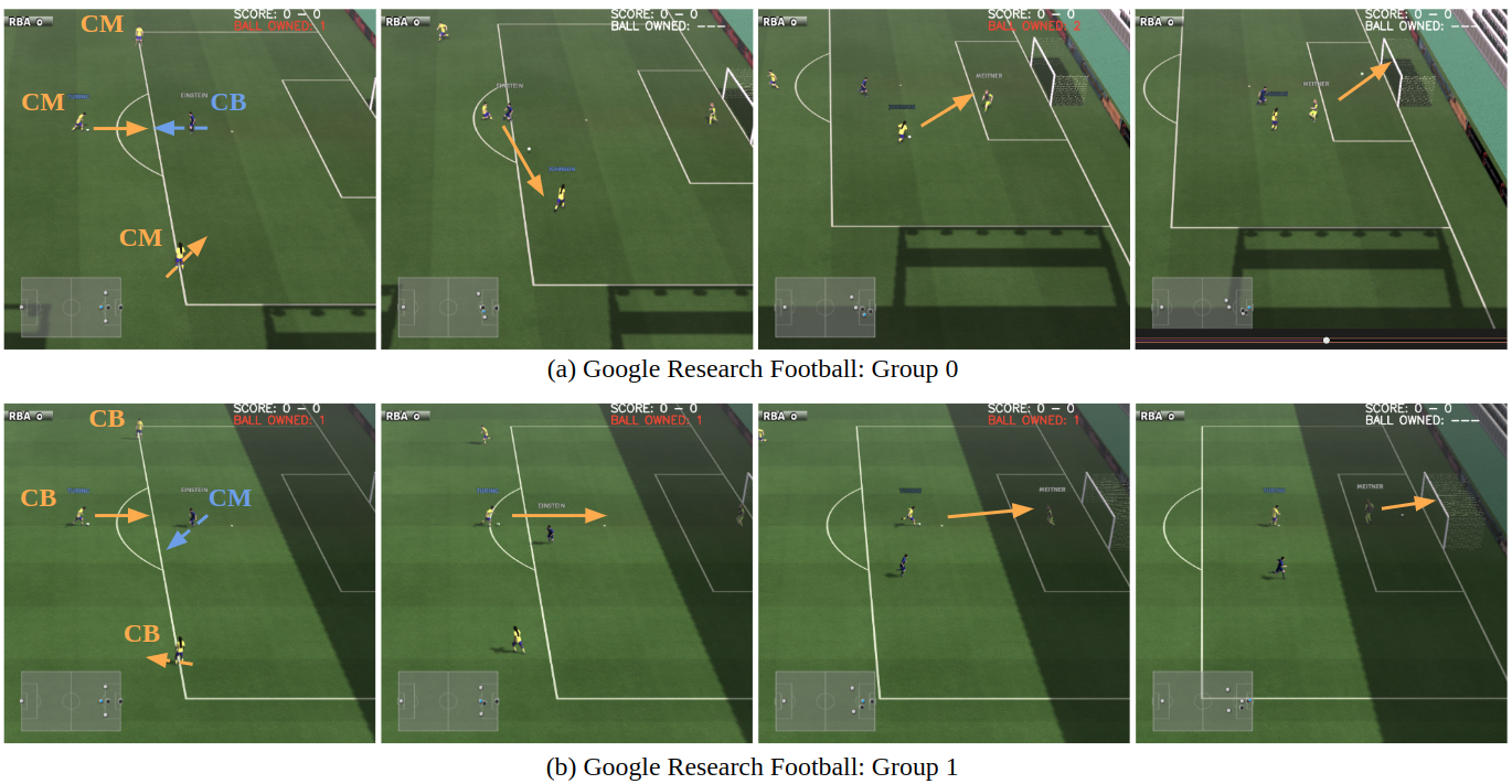
Figure 6: This figure displays good solutions for tasks from two groups in GRF 3 vs. 2. The yellow solid arrow depicts the movement direction of the ball, the yellow dashed arrow depicts the movement direction of the attacking player on the wing, and the blue dashed arrow shows the movement direction of the defending player.

Table 2: Observation and action space in Google Research Football

Dim.	Continuous Observation Space	range
0-7	$x,y$ positions of the attacking players (including the goalkeeper)	$[-1,1]$
8-11	$x,y$ positions of the defending players	$[-1,1]$
12-19	movements of the attacking players along $x,y$ directions	$[-1,1]$
20-23	movements of the defending players along $x,y$ directions	$[-1,1]$
24-26	$x,y,z$ positions of the ball	$[-\inf,\inf]$
27-29	movements of the ball along $x,y,z$ directions	$[-1,1]$
30-32	$x,y,z$ rotation angles of the ball in radians	$[-\pi,\pi]$
33-35	the one-hot encoding denoting the team controlling the ball	$\{0,1\}$
36-40	the one-hot encoding denoting the player controlling the ball	$\{0,1\}$
41-42	scores for each team (an episode terminates when any team scores)	$\{0,1\}$
43-46	the one-hot encoding denoting the active player controlled by RL	$\{0,1\}$
47-56	10-elements vectors of 0s or 1s denoting whether a sticky action is active	$\{0,1\}$
Index	Discrete Action Space
0	idle
1	run to the left, sticky action
2	run to the top-left, sticky action
3	run to the top, sticky action
4	run to the top-right, sticky action
5	run to the right, sticky action
6	run to the bottom-right, sticky action
7	run to the bottom, sticky action
8	run to the bottom-left, sticky action
9	perform a long pass
10	perform a high pass
11	perform a short pass
12	perform a shot
13	start sprinting, sticky action
14	reset current movement direction
15	stop sprinting
16	perform a slide
17	start dribbling, sticky action
18	stop dribbling

Table 3: Detailed task descriptions for Google Research Football

Task Index	Parameter 1	Parameter 2	Group Index	Probability
	Player Type	Player Capability Level
0	CM vs. CB	0.9 vs. 0.6	0	0.5
1	CM vs. CB	1.0 vs. 0.7	0	0.5
2	CB vs. CM	0.9 vs. 0.6	1	0.5
3	CB vs. CM	1.0 vs. 0.7	1	0.5

C.2 LunarLander

We modify the LunarLander environment [68] by changing the engine mode and engine power. The mixture index set ${\mathcal{Z}}$ has a cardinality of two, $z=0$ and $z=1$, corresponding to two different engine operation modes, normal mode and left-right-flip mode, respectively. When in left-right-flip mode, the action turning on the left engine in normal mode will turn on the right engine instead, and the action turning on the right engine in normal mode will turn on the left instead. We visualize the tasks in Figure 7. The engine power has two choices which are 3.0 and 6.0. The MDP set ${\mathcal{M}}$ has carnality four corresponding to four combinations of engine mode and engine power. Detailed descriptions of the state and action space are shown in Table 5.

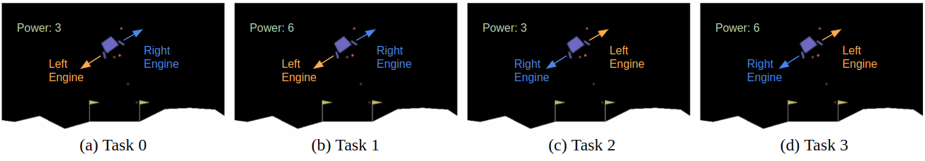
Figure 7: LunarLander task visualization. Task 0 and task 1 belong to group 0 (normal mode). Tasks 2 and task 3 belong to group 1 (flip mode).

Table 4: Detailed task descriptions for LunarLander

Task Index	Parameter 1	Parameter 2	Group Index	Probability
	Engine Mode	Engine Power
0	Normal	3.0	0	0.5
1	Normal	6.0	0	0.5
2	Flipped	3.0	1	0.5
3	Flipped	6.0	1	0.5

Table 5: Observation and action space in LunarLander

Dim.	Continuous Observation Space	range
0	$x$ position	$[-\inf,\inf]$
1	$y$ position	$[-\inf,\inf]$
2	$x$ velocity	$[-\inf,\inf]$
3	$y$ velocity (relative): $x,y,v_{x},v_{y}$	$[-\inf,\inf]$
4	angle	$[-\pi,\pi]$
5	angular velocity	$[-\inf,\inf]$
6	if left leg contact with ground	$\{0,1\}$
7	if right leg contact with ground	$\{0,1\}$
Index	Discrete Action Space
0	idle
1	turn on left engine (normal mode)/Turn on right engine (left-right-flip mode)
2	turn on main engine
3	turn on right engine (normal mode)/Turn on left engine (left-right-flip mode)

C.3 HalfCheetah

We modify the joint failure and torso mass of HalfCheetah and build 18 tasks with different dynamics. The joint failure has six choices which correspond to the 6 joints of HalfCheetah. For instance, when the joint failure index is 0, we cannot apply control torque (action) to joint 0. The torso mass has three choices, which are 0.9, 1.0, and 1.1 times the original torso mass. We visualize the joint indexes in Figure 8. Detailed descriptions of the state and action space are shown in Table 6.

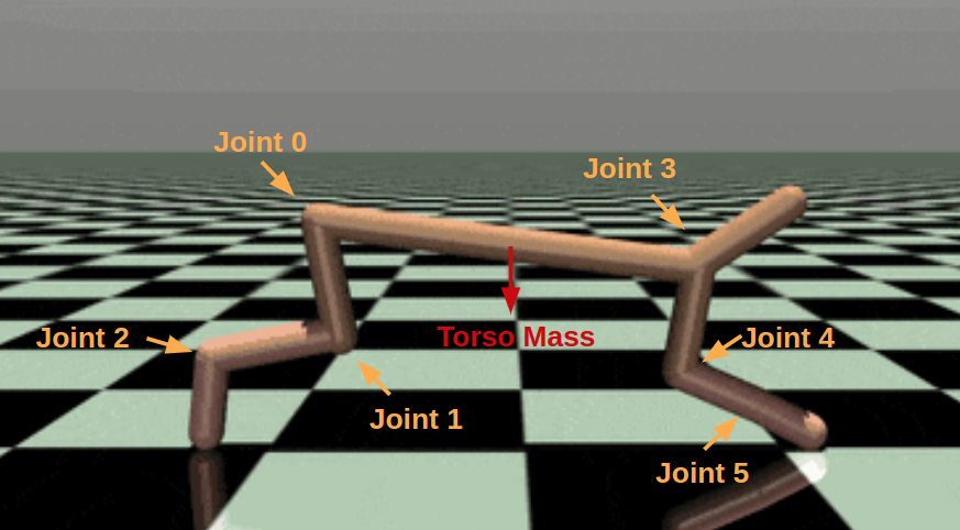
Figure 8: HalfCheetah visualization.

Table 6: Observation and action space in HalfCheetah

Dim.	Continuous Observation Space
0-8	positional information
9-16	velocity information
Dim	Continuous Action Space
0-5	control torque

Table 7: Detailed task descriptions for HalfCheetah

Task Index	Parameter 1	Parameter 2	Group Index	Probability
	Failure Joint	Torso Mass
0	0	0.9	0	$1/3$
1	0	1.0	0	$1/3$
2	0	1.1	0	$1/3$
3	1	0.9	1	$1/3$
4	1	1.0	1	$1/3$
5	1	1.1	1	$1/3$
6	2	0.9	2	$1/3$
7	2	1.0	2	$1/3$
8	2	1.1	2	$1/3$
9	3	0.9	3	$1/3$
10	3	1.0	3	$1/3$
11	3	1.1	3	$1/3$
12	4	0.9	4	$1/3$
13	4	1.0	4	$1/3$
14	4	1.1	4	$1/3$
15	5	0.9	5	$1/3$
16	5	1.0	5	$1/3$
17	5	1.1	5	$1/3$

Appendix D Implementation Details

Trajectory rollout.

In both training and testing, we initialize the environment by sampling first a mixture and then an MDP realization. The sampled mixture and MDP are fixed throughout one episode. In our environments with discrete mixtures and MDPs, we can represent the ground truth mixture index $\hat{z}$ with a one-hot vector $e_{\hat{z}}$, which is used in the pretraining phase of all baselines and in the whole training phase of baseline G-Exact. For baselines with belief module including GDR, G-Belief, DR, State-R, the actual mixture $\hat{z}$ and MDP weights $\mu(m|\hat{z})$ are unknown to the RL agent. Instead, the RL agent is given the number of possible mixtures $Z$ and is able to infer a belief over mixtures $b(z)$ based on a belief update function $SE$. A detailed algorithm for trajectory rollout is Algorithm 1. For baseline No-Belief, we mask out the beliefs in the input by replacing them with zeros.

Belief update mechanism.

In our implementation (Section 7), we use the Bayesian update rule to update beliefs based on the interaction at each timestep. At the beginning of each episode, we initialize a uniform belief distribution $b_{0}(i)=1/(|{\mathcal{Z}}|),\forall i\in[|{\mathcal{Z}}|]$. At timestep $t$, we update the belief as follows

$$b_{t+1}(j)=\frac{b_{t}(j)L(j)}{\sum_{i\in[|{\mathcal{Z}}|]}b_{t}(i)L(i)},\forall j\in[|{\mathcal{Z}}|],$$

where $L$ represents the likelihood. Let $\hat{z}$ denote the true mixture index for the episode. We let the likelihood $L$ vector be a soft version of the actual one-hot mixture encoding $e_{\hat{z}}$.

More concretely, at each time step, we first sample a noisy index $j$ where $j=\hat{z}$ with probability $\epsilon_{l}$ and $j$ is uniformly sampled from $[Z]$ otherwise. The likelihood $L$ is a vector with dimension $|{\mathcal{Z}}|$, and $\forall i\in[|{\mathcal{Z}}|]$, the $i$-th element $L(i)$ is

$$L(i)=\begin{cases}l,&\text{if }i=j\\ (1-l)/(|{\mathcal{Z}}|-1),&\text{if }i\not=j\end{cases}$$

There are lots of literature on accurate belief updates [72]. In this work, we utilize a simple but controllable belief update mechanism above, which is more suitable for robustness evaluations since we could explicitly vary the hyperparameters. We leave a more sophisticated design of belief update mechanism for future work.

Belief noise level

During robustness evaluation in Section 8, we control the belief noise level $\epsilon_{\hat{z}}$ which affects the likelihood $L$. More concretely, we add another layer of randomness on the estimate of $\hat{z}$. Define the noisy mixture index at test-time as $z_{text}$, we have

$$z_{test}=\begin{cases}\hat{z}&\text{with probability }\epsilon_{\hat{z}}\\ \text{a random index uniforms samples from }[|{\mathcal{Z}}|],&\text{otherwise}\end{cases}$$

During the robust evaluation, the likelihood $L_{test}$ is calculated based on $z_{test}$. More concretely, at each time step, we first sample a noisy index $j$ where $j=z_{test}$ with probability $\epsilon_{l}$ and $j$ is uniformly sampled from $[Z]$ otherwise. The likelihood and belief updates are as follows:

$$L_{test}(i)=\begin{cases}l,&\text{if }i=j\\ (1-l)/(|{\mathcal{Z}}|-1),&\text{if }i\not=j\end{cases},\text{ and }b_{t+1}(j)=\frac{b_{t}(j)L_{test}(j)}{\sum_{i\in[|{\mathcal{Z}}|]}b_{t}(i)L_{test}(i)},\forall j\in[|{\mathcal{Z}}|].$$

Distributionally robust training with belief distribution over MDPs (DR)

DR has an agent that takes the belief distribution $b(m)$ and state $s$ as inputs. DR uses the same belief updating rule as in GDR to update $b(z)$ at each timestep and then project $b(z)$ to $b(m)$ with $\mu_{z}(m)$.

This is a variant of our proposed Group Distributionally Robust DQN, which has a perturbed target taking $m$-level belief distribution as part of its input. Note that in DR, we still update $z$-level belief $b(z)$ based on the same belief updating function $SE$ as in GDR. However, in DR, for data pair $d$, the ambiguity set ${\mathcal{C}}_{b^{\prime}(m),d_{TV},\xi}$ is centered at $b^{\prime}(m)=T_{{\bm{A}}}(b^{\prime}(z))$ which is mapped from $b^{\prime}(z)$. We also modify the fast gradient sign attack over $b(m)$ accordingly. We first sample $i\in[M]$ and apply attacks as $p(m)_{j}=p(m)_{j}+\alpha_{b}\cdot\operatorname{sign}(\nabla_{p(m),j}V(p(m),s^{\prime})),\ \forall j\not=i$ and $p(m)_{i}=p(m)_{i}-\sum_{j\not=i}p(m)_{j}$. We iteratively apply the gradient sign attack to find $b^{adv}(m)=\operatorname*{arg\,min}_{\begin{subarray}{c}p(m)\in{\mathcal{C}}_{b^{\prime}(m),d_{TV},\xi}\end{subarray}}\sum_{a\in{\mathcal{A}}}Q_{\theta}(p(m),s^{\prime},a)$.

D.1 GDR-PPO

We represent the pseudo algorithm of GDR-PPO in Algorithm 3. We collect rollouts with un-perturbed beliefs and use the online rollouts to update the value network. To enhance the robustness to belief ambiguity, we tend to down-weight the probability of trajectories that may lead to large performance drops under the worst-possible belief within the ambiguity set. Hence we construct a pseudo-advantage $\hat{A}$ by subtracting the performance drop $R_{drop}$ from the actual accumulated return. The worst-possible belief is calculated by FGSM.

Input: Value-net $V_{\theta}(b(z),s)$, ambiguity set ${\mathcal{C}}_{\cdot,d_{TV},\xi}$, training episodes $N$

Initialize data buffer ${\mathcal{D}}$ ;

for $n=0$ to $N$ do

       Rollout several episode with Algorithm 1 and append data pairs to ${\mathcal{D}}$ ;

       if Update Actor-net parameters then

             Sample batch data from ${\mathcal{D}}$ ;

             for Each trajectory in the batch do

                   Get advantage for the data pair at timestep $t$ $\hat{A}(b_{t},s_{t})=\sum_{t^{\prime}=t}^{T-1}r_{t}-\Big{(}V(b_{t},s_{t})-\min_{\begin{subarray}{c}p(z)\in{\mathcal{C}}_{b_{t}(z),d_{TV},\xi}\end{subarray}}V_{\theta}(p(z),s_{t})\Big{)}-V_{\theta}(b_{t},s_{t})$ ;

                  

            Update Actor-net with PPO ;

            

Return: Actor-net

Algorithm 3 Group Distributionally Robust Training for GDR-PPO

D.2 Hyperparameters

We show the hyperparameters for training Google Research Football, Lunarlander and Halfcheetah in Table 8, Table 9 and Table 10, respectively. We select hyperparameters via grid search.

Table 8: Hyperparameters for the Google Research Football

reward decay	0.997
net hidden structure	$[256,256]$
net activation function	Tanh
learning rate	0.00012
GAE ($\lambda$)	0.95
clipping range	0.115
entropy coefficient	0.00155
value function coefficient	0.5
number of environment steps per update	8192
epoch	10
adv budget	0.2
adv step size	0.1
adv max step	10
batch size	256

Table 9: Hyperparameters for the LunarLander task

reward decay	0.95
net hidden structure	$[128,128]$
net activation function	ReLU
value function learning rate	0.01
value function learning rate decay	0.999
epoch	20
gradient steps per epoch	5000
adv budget	0.4
adv step size	0.02
adv max step	50
batch size	256

Table 10: Hyperparameters for the Halfcheetah

reward decay	0.99
net hidden structure	$[256,256]$
net activation function	ReLU
value function learning rate	0.001
value function learning rate decay	0.999
epoch	200
gradient steps per epoch	5000
adv budget	0.2
adv step size	0.02
adv max step	50
batch size	256

Appendix E Additional Ablation Study

In this section, we show how the ambiguity set size and the pretrain episodes affect the training stability and robustness of DR, which maintains a belief over MDPs. Compared with our proposed GDR, DR omits the hierarchical structure.

E.1 The effect of Ambiguity Set Size

Figure 9 shows the effect of the ambiguity set in HalfCheetah. All curves in Figure 9 are pre-trained in the first 100000 episodes. With ambiguity set size 0.01 and 0.05, the DR does not crash and converge to a non-negative value. Comparing Figure 9 (b) for DR with Figure 3 (c) for GDR, we can conclude that GDR is less sensitive to the ambiguity set size along training since it converge to a non-negative value with a larger range of ambiguity set size. Comparing Figure 5 (a) with Figure 4 (c) for our proposed GDR, we can conclude that the hierarchical structure enhances the robustness to belief noise since the robustness performance for GDR consistently outperforms that of DR for different ambiguity set sizes.

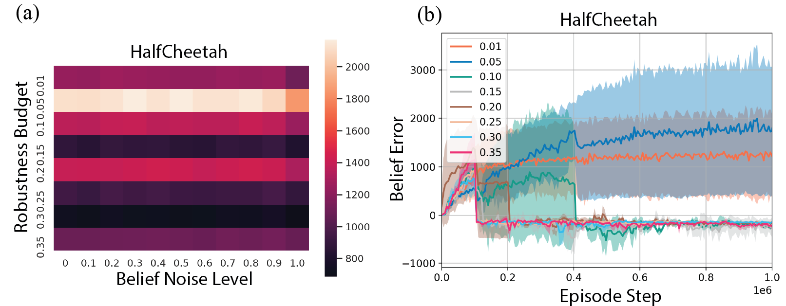
Figure 9: Ablation study about the effect of ambiguity set budget on DR’s robustness and training stability. We choose the ambiguity set size among 0.01, 0.05, 0.1, 0.15, 0.2, 0.25, 0.3, and 0.35.

E.2 The effect of Pretrain Episodes

Figure 10 shows the effect of the pretrain episodes in HalfCheetah. All curves in Figure 10 has an ambiguity set size 0.2. Figure 10 shows that even pretraining for 900000 episodes, DR still will crash after the pretraining phase. It shows that DR is less sensitive to the pretraining episodes compared with the ambiguity set size.

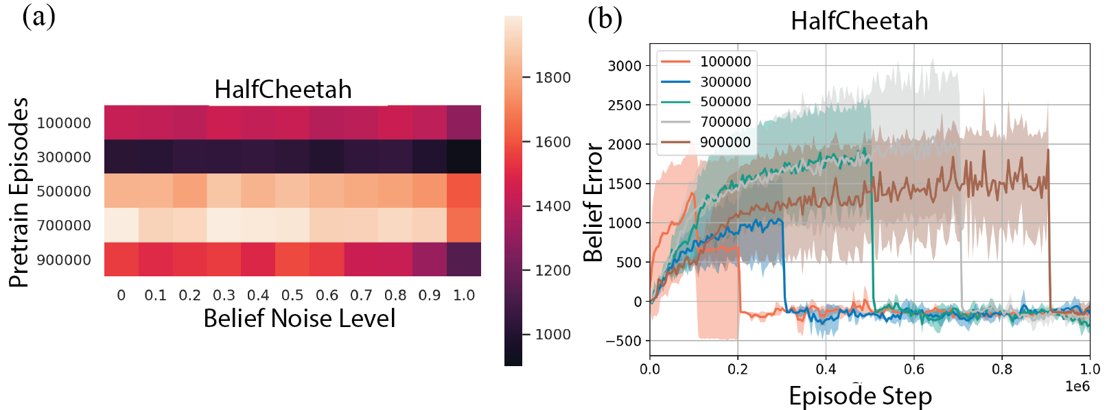
Figure 10: Ablation study about the effect of pretrain episodes on DR’s robustness and training stability. We choose the number of pretrain episodes among 100000, 300000, 500000, 700000, and 900000.

References

- [1] Volodymyr Mnih, Koray Kavukcuoglu, David Silver, Alex Graves, Ioannis Antonoglou, Daan Wierstra, and Martin Riedmiller. Playing atari with deep reinforcement learning. arXiv preprint arXiv:1312.5602, 2013.
- [2] Jens Kober, J Andrew Bagnell, and Jan Peters. Reinforcement learning in robotics: A survey. The International Journal of Robotics Research, 32(11):1238–1274, 2013.
- [3] Robert Kirk, Amy Zhang, Edward Grefenstette, and Tim Rocktäschel. A survey of generalisation in deep reinforcement learning. arXiv preprint arXiv:2111.09794, 2021.
- [4] Chelsea Finn, Pieter Abbeel, and Sergey Levine. Model-agnostic meta-learning for fast adaptation of deep networks. In International conference on machine learning, pages 1126–1135. PMLR, 2017.
- [5] Lauren N Steimle, David L Kaufman, and Brian T Denton. Multi-model markov decision processes. IISE Transactions, pages 1–16, 2021.
- [6] Shagun Sodhani, Amy Zhang, and Joelle Pineau. Multi-task reinforcement learning with context-based representations. In International Conference on Machine Learning, pages 9767–9779. PMLR, 2021.
- [7] Aaron Wilson, Alan Fern, Soumya Ray, and Prasad Tadepalli. Multi-task reinforcement learning: a hierarchical bayesian approach. In Proceedings of the 24th international conference on Machine learning, pages 1015–1022, 2007.
- [8] Kate Rakelly, Aurick Zhou, Chelsea Finn, Sergey Levine, and Deirdre Quillen. Efficient off-policy meta-reinforcement learning via probabilistic context variables. In International conference on machine learning, pages 5331–5340. PMLR, 2019.
- [9] Karol Hausman, Jost Tobias Springenberg, Ziyu Wang, Nicolas Heess, and Martin Riedmiller. Learning an embedding space for transferable robot skills. In International Conference on Learning Representations, 2018.
- [10] Annie Xie, Shagun Sodhani, Chelsea Finn, Joelle Pineau, and Amy Zhang. Robust policy learning over multiple uncertainty sets. arXiv preprint arXiv:2202.07013, 2022.
- [11] Apoorva Sharma, James Harrison, Matthew Tsao, and Marco Pavone. Robust and adaptive planning under model uncertainty. In Proceedings of the International Conference on Automated Planning and Scheduling, volume 29, pages 410–418, 2019.
- [12] Arnab Nilim and Laurent El Ghaoui. Robust control of markov decision processes with uncertain transition matrices. Operations Research, 53(5):780–798, 2005.
- [13] Garud N Iyengar. Robust dynamic programming. Mathematics of Operations Research, 30(2):257–280, 2005.
- [14] Kaiqing Zhang, Bin Hu, and Tamer Basar. On the stability and convergence of robust adversarial reinforcement learning: A case study on linear quadratic systems. Advances in Neural Information Processing Systems, 33, 2020.
- [15] Jing Yu, Clement Gehring, Florian Schäfer, and Animashree Anandkumar. Robust reinforcement learning: A constrained game-theoretic approach. In Learning for Dynamics and Control, pages 1242–1254. PMLR, 2021.
- [16] Peide Huang, Mengdi Xu, Fei Fang, and Ding Zhao. Robust reinforcement learning as a stackelberg game via adaptively-regularized adversarial training. arXiv preprint arXiv:2202.09514, 2022.
- [17] Wenhao Yu, Jie Tan, C Karen Liu, and Greg Turk. Preparing for the unknown: Learning a universal policy with online system identification. arXiv preprint arXiv:1702.02453, 2017.
- [18] Johanna Etner, Meglena Jeleva, and Jean-Marc Tallon. Decision theory under ambiguity. Journal of Economic Surveys, 26(2):234–270, 2012.
- [19] Daniel Ellsberg. Risk, ambiguity, and the savage axioms. The quarterly journal of economics, pages 643–669, 1961.
- [20] Mark J Machina and Marciano Siniscalchi. Ambiguity and ambiguity aversion. In Handbook of the Economics of Risk and Uncertainty, volume 1, pages 729–807. Elsevier, 2014.
- [21] Hamed Rahimian and Sanjay Mehrotra. Distributionally robust optimization: A review. arXiv preprint arXiv:1908.05659, 2019.
- [22] Daniel Kuhn, Peyman Mohajerin Esfahani, Viet Anh Nguyen, and Soroosh Shafieezadeh-Abadeh. Wasserstein distributionally robust optimization: Theory and applications in machine learning. In Operations Research & Management Science in the Age of Analytics, pages 130–166. INFORMS, 2019.
- [23] Wolfram Wiesemann, Daniel Kuhn, and Berç Rustem. Robust markov decision processes. Mathematics of Operations Research, 38(1):153–183, 2013.
- [24] Takayuki Osogami. Robust partially observable markov decision process. In International Conference on Machine Learning, pages 106–115. PMLR, 2015.
- [25] Chen Tessler, Yonathan Efroni, and Shie Mannor. Action robust reinforcement learning and applications in continuous control. In International Conference on Machine Learning, pages 6215–6224. PMLR, 2019.
- [26] Huan Zhang, Hongge Chen, Chaowei Xiao, Bo Li, Mingyan Liu, Duane Boning, and Cho-Jui Hsieh. Robust deep reinforcement learning against adversarial perturbations on state observations. arXiv preprint arXiv:2003.08938, 2020.
- [27] Janosch Moos, Kay Hansel, Hany Abdulsamad, Svenja Stark, Debora Clever, and Jan Peters. Robust reinforcement learning: A review of foundations and recent advances. Machine Learning and Knowledge Extraction, 4(1):276–315, 2022.
- [28] Peter Klibanoff, Massimo Marinacci, and Sujoy Mukerji. A smooth model of decision making under ambiguity. Econometrica, 73(6):1849–1892, 2005.
- [29] Jakob N Foerster, Richard Y Chen, Maruan Al-Shedivat, Shimon Whiteson, Pieter Abbeel, and Igor Mordatch. Learning with opponent-learning awareness. arXiv preprint arXiv:1709.04326, 2017.
- [30] Lerrel Pinto, James Davidson, Rahul Sukthankar, and Abhinav Gupta. Robust adversarial reinforcement learning. In International Conference on Machine Learning, pages 2817–2826. PMLR, 2017.
- [31] Kaiqing Zhang, TAO SUN, Yunzhe Tao, Sahika Genc, Sunil Mallya, and Tamer Basar. Robust multi-agent reinforcement learning with model uncertainty. In H. Larochelle, M. Ranzato, R. Hadsell, M. F. Balcan, and H. Lin, editors, Advances in Neural Information Processing Systems, volume 33, pages 10571–10583. Curran Associates, Inc., 2020.
- [32] Huan Xu and Shie Mannor. Distributionally robust markov decision processes. In NIPS, pages 2505–2513, 2010.
- [33] Pengqian Yu and Huan Xu. Distributionally robust counterpart in markov decision processes. IEEE Transactions on Automatic Control, 61(9):2538–2543, 2015.
- [34] Elena Smirnova, Elvis Dohmatob, and Jérémie Mary. Distributionally robust reinforcement learning. arXiv preprint arXiv:1902.08708, 2019.
- [35] Julien Grand-Clément and Christian Kroer. First-order methods for wasserstein distributionally robust mdp. arXiv preprint arXiv:2009.06790, 2020.
- [36] Zhengqing Zhou, Zhengyuan Zhou, Qinxun Bai, Linhai Qiu, Jose Blanchet, and Peter Glynn. Finite-sample regret bound for distributionally robust offline tabular reinforcement learning. In International Conference on Artificial Intelligence and Statistics, pages 3331–3339. PMLR, 2021.
- [37] Hideaki Nakao, Ruiwei Jiang, and Siqian Shen. Distributionally robust partially observable markov decision process with moment-based ambiguity. SIAM Journal on Optimization, 31(1):461–488, 2021.
- [38] Aman Sinha, Matthew O’Kelly, Hongrui Zheng, Rahul Mangharam, John Duchi, and Russ Tedrake. Formulazero: Distributionally robust online adaptation via offline population synthesis. In International Conference on Machine Learning, pages 8992–9004. PMLR, 2020.
- [39] Erick Delage and Yinyu Ye. Distributionally robust optimization under moment uncertainty with application to data-driven problems. Oper. Res., 58:595–612, 2010.
- [40] Mohammad Ghavamzadeh, Shie Mannor, Joelle Pineau, Aviv Tamar, et al. Bayesian reinforcement learning: A survey. Foundations and Trends® in Machine Learning, 8(5-6):359–483, 2015.
- [41] Emma Brunskill. Bayes-optimal reinforcement learning for discrete uncertainty domains. In Proceedings of the 11th International Conference on Autonomous Agents and Multiagent Systems-Volume 3, pages 1385–1386, 2012.
- [42] Arthur Guez, David Silver, and Peter Dayan. Efficient bayes-adaptive reinforcement learning using sample-based search. Advances in neural information processing systems, 25, 2012.
- [43] Gilwoo Lee, Brian Hou, Aditya Mandalika, Jeongseok Lee, Sanjiban Choudhury, and Siddhartha S Srinivasa. Bayesian policy optimization for model uncertainty. arXiv preprint arXiv:1810.01014, 2018.
- [44] Mengdi Xu, Zuxin Liu, Peide Huang, Wenhao Ding, Zhepeng Cen, Bo Li, and Ding Zhao. Trustworthy reinforcement learning against intrinsic vulnerabilities: Robustness, safety, and generalizability. arXiv preprint arXiv:2209.08025, 2022.
- [45] Jeongyeol Kwon, Yonathan Efroni, Constantine Caramanis, and Shie Mannor. Rl for latent mdps: Regret guarantees and a lower bound. arXiv preprint arXiv:2102.04939, 2021.
- [46] Assaf Hallak, Dotan Di Castro, and Shie Mannor. Contextual markov decision processes. ArXiv, abs/1502.02259, 2015.
- [47] Finale Doshi-Velez and George Konidaris. Hidden parameter markov decision processes: A semiparametric regression approach for discovering latent task parametrizations. In IJCAI: proceedings of the conference, volume 2016, page 1432. NIH Public Access, 2016.
- [48] Emma Brunskill and Lihong Li. Sample complexity of multi-task reinforcement learning. arXiv preprint arXiv:1309.6821, 2013.
- [49] Leslie Pack Kaelbling, Michael L Littman, and Anthony R Cassandra. Planning and acting in partially observable stochastic domains. Artificial intelligence, 101(1-2):99–134, 1998.
- [50] Joey Hong, Branislav Kveton, Manzil Zaheer, and Mohammad Ghavamzadeh. Hierarchical bayesian bandits. arXiv preprint arXiv:2111.06929, 2021.
- [51] Mengdi Xu, Wenhao Ding, Jiacheng Zhu, Zuxin Liu, Baiming Chen, and Ding Zhao. Task-agnostic online reinforcement learning with an infinite mixture of gaussian processes. Advances in Neural Information Processing Systems, 33:6429–6440, 2020.
- [52] Peter Karkus, David Hsu, and Wee Sun Lee. Qmdp-net: Deep learning for planning under partial observability. arXiv preprint arXiv:1703.06692, 2017.
- [53] Shiori Sagawa, Pang Wei Koh, Tatsunori B Hashimoto, and Percy Liang. Distributionally robust neural networks for group shifts: On the importance of regularization for worst-case generalization. arXiv preprint arXiv:1911.08731, 2019.
- [54] Yonatan Oren, Shiori Sagawa, Tatsunori B Hashimoto, and Percy Liang. Distributionally robust language modeling. arXiv preprint arXiv:1909.02060, 2019.
- [55] Linwei Xin and David A Goldberg. Time (in) consistency of multistage distributionally robust inventory models with moment constraints. European Journal of Operational Research, 289(3):1127–1141, 2021.
- [56] Shie Mannor, Ofir Mebel, and Huan Xu. Robust mdps with k-rectangular uncertainty. Mathematics of Operations Research, 41(4):1484–1509, 2016.
- [57] Vineet Goyal and Julien Grand-Clement. Robust markov decision process: Beyond rectangularity. arXiv preprint arXiv:1811.00215, 2018.
- [58] Stefan Banach. Sur les opérations dans les ensembles abstraits et leur application aux équations intégrales. Fund. math, 3(1):133–181, 1922.
- [59] Mohammed Amin Abdullah, Hang Ren, Haitham Bou Ammar, Vladimir Milenkovic, Rui Luo, Mingtian Zhang, and Jun Wang. Wasserstein robust reinforcement learning. arXiv preprint arXiv:1907.13196, 2019.
- [60] Aman Sinha, Hongseok Namkoong, Riccardo Volpi, and John Duchi. Certifying some distributional robustness with principled adversarial training. arXiv preprint arXiv:1710.10571, 2017.
- [61] Erwan Lecarpentier and Emmanuel Rachelson. Non-stationary markov decision processes, a worst-case approach using model-based reinforcement learning, extended version. arXiv preprint arXiv:1904.10090, 2019.
- [62] Matthew Staib and Stefanie Jegelka. Distributionally robust deep learning as a generalization of adversarial training. In NIPS workshop on Machine Learning and Computer Security, 2017.
- [63] Tuomas Haarnoja, Aurick Zhou, Pieter Abbeel, and Sergey Levine. Soft actor-critic: Off-policy maximum entropy deep reinforcement learning with a stochastic actor. In International conference on machine learning, pages 1861–1870. PMLR, 2018.
- [64] John Schulman, Filip Wolski, Prafulla Dhariwal, Alec Radford, and Oleg Klimov. Proximal policy optimization algorithms. arXiv preprint arXiv:1707.06347, 2017.
- [65] Jiayi Weng, Huayu Chen, Dong Yan, Kaichao You, Alexis Duburcq, Minghao Zhang, Hang Su, and Jun Zhu. Tianshou: A highly modularized deep reinforcement learning library. arXiv preprint arXiv:2107.14171, 2021.
- [66] Antonin Raffin, Ashley Hill, Adam Gleave, Anssi Kanervisto, Maximilian Ernestus, and Noah Dormann. Stable-baselines3: Reliable reinforcement learning implementations. Journal of Machine Learning Research, 22(268):1–8, 2021.
- [67] Ian J Goodfellow, Jonathon Shlens, and Christian Szegedy. Explaining and harnessing adversarial examples. arXiv preprint arXiv:1412.6572, 2014.
- [68] Greg Brockman, Vicki Cheung, Ludwig Pettersson, Jonas Schneider, John Schulman, Jie Tang, and Wojciech Zaremba. Openai gym. arXiv preprint arXiv:1606.01540, 2016.
- [69] Emanuel Todorov, Tom Erez, and Yuval Tassa. Mujoco: A physics engine for model-based control. In 2012 IEEE/RSJ international conference on intelligent robots and systems, pages 5026–5033. IEEE, 2012.
- [70] Karol Kurach, Anton Raichuk, Piotr Stańczyk, Michał Zajac, Olivier Bachem, Lasse Espeholt, Carlos Riquelme, Damien Vincent, Marcin Michalski, Olivier Bousquet, et al. Google research football: A novel reinforcement learning environment. In Proceedings of the AAAI Conference on Artificial Intelligence, volume 34, pages 4501–4510, 2020.
- [71] Daniel P Heyman and Matthew J Sobel. Stochastic models in operations research: stochastic optimization, volume 2. Courier Corporation, 2004.
- [72] Samuel Sokota, Hengyuan Hu, David J Wu, J Zico Kolter, Jakob Nicolaus Foerster, and Noam Brown. A fine-tuning approach to belief state modeling. In International Conference on Learning Representations, 2021.