Score-based Denoising Diffusion with
Non-Isotropic Gaussian Noise Models

Abstract

Generative models based on denoising diffusion techniques have led to an unprecedented increase in the quality and diversity of imagery that is now possible to create with neural generative models. However, most contemporary state-of-the-art methods are derived from a standard isotropic Gaussian formulation. In this work we examine the situation where non-isotropic Gaussian distributions are used. We present the key mathematical derivations for creating denoising diffusion models using an underlying non-isotropic Gaussian noise model. We also provide initial experiments with the CIFAR10 dataset to help verify empirically that this more general modelling approach can also yield high-quality samples.

1 Introduction

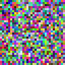
(a) Isotropic

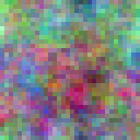
(b) Non-isotropic

Figure 1: Gaussian noise samples.

Score-based denoising diffusion models [16, 6, 18] have seen great success as generative models for images [4, 17], as well as other modes such as video [7, 22, 19], audio [9, 3], etc. The underlying framework relies on a noising "forward" process that adds noise to real images (or other data), and a denoising "reverse" process that iteratively removes noise. In most cases, the noise distribution used is the isotropic Gaussian i.e. noise samples are independently and identically distributed (IID) as the standard normal at each pixel.

In this work, we lay the theoretical foundations and derive the key mathematics for a non-isotropic Gaussian formulation for denoising diffusion models. It is our hope that these insights may open the door to new classes of models. One type of non-isotropic Gaussian noise arises in a family of models known as Gaussian Free Fields (GFFs) [14, 1, 2, 20] (a.k.a. Gaussian Random Fields). GFF noise can be obtained by either convolving isotropic Gaussian noise with a filter, or applying frequency masking of noise. In either case this procedure allows one to model or generate smoother and correlated types of Gaussian noise. In Figures 1 and 2, we compare examples of isotropic Gaussian noise with GFF noise obtained using a frequency space window function consisting of $w(f)=\frac{1}{f}$.

Our contributions here consist of the following: (1) deriving the key mathematics for score-based denoising diffusion models using non-isotropic multivariate Gaussian distributions, (2) examining the special case of a GFF and the corresponding non-Isotropic Gaussian noise model, and (3) showing that diffusion models trained (eg. on the CIFAR-10 dataset [10]) using a GFF noise process are also capable of yielding high-quality samples comparable to models based on isotropic Gaussian noise.

Appendix A and Appendix B contain more detailed derivations of the above equations for DDPM [6] and our NI-DDPM. See Appendix D and Appendix E for the equivalent derivations for Score Matching Langevin Dynamics (SMLD) [16, 17], and our Non-Isotropic SMLD (NI-SMLD).

2 Isotropic Gaussian denoising diffusion models

We perform our analysis below within the Denoising Diffusion Probabilistic Models (DDPM) [6] framework, but our analysis is valid for all other types of score-based denoising diffusion models.

In DDPM, for a fixed sequence of positive scales $0<\beta_{1}<\cdots<\beta_{L}<1$, $\bar{\alpha}_{t}=\prod_{s=1}^{t}(1-\beta_{s})$, and a noise sample ${\bm{\epsilon}}\sim{\mathcal{N}}({\bm{0}},{\mathbf{I}})$, the cumulative “forward” noising process is:

$$q_{t}({\mathbf{x}}_{t}\mid{\mathbf{x}}_{0})={\mathcal{N}}(\sqrt{\bar{\alpha}_{t}}{\mathbf{x}}_{0},(1-\bar{\alpha}_{t}){\mathbf{I}})\implies{\mathbf{x}}_{t}=\sqrt{\bar{\alpha}_{t}}{\mathbf{x}}_{0}+\sqrt{1-\bar{\alpha}_{t}}{\bm{\epsilon}}$$ (1)

The “reverse” process involves iteratively sampling ${\mathbf{x}}_{t-1}$ from ${\mathbf{x}}_{t}$ conditioned on ${\mathbf{x}}_{0}$ i.e. $p_{t-1}({\mathbf{x}}_{t-1}\mid{\mathbf{x}}_{t},{\mathbf{x}}_{0})$, obtained from $q_{t}({\mathbf{x}}_{t}\mid{\mathbf{x}}_{0})$ using Bayes’ rule. For this, first ${\bm{\epsilon}}$ is estimated using a neural network ${\bm{\epsilon}}_{\bm{\theta}}({\mathbf{x}}_{t},t)$. Then, using $\hat{\mathbf{x}}_{0}=\big{(}{\mathbf{x}}_{t}-\sqrt{1-\bar{\alpha}_{t}}{\bm{\epsilon}}_{{\bm{\theta}}}({\mathbf{x}}_{t},t)\big{)}/\sqrt{\bar{\alpha}_{t}}$ from eq. 1, ${\mathbf{x}}_{t-1}$ is sampled:

$$p_{t-1}({\mathbf{x}}_{t-1}\mid{\mathbf{x}}_{t},\hat{{\mathbf{x}}}_{0})={\mathcal{N}}(\ \tilde{\bm{\mu}}_{t}({\mathbf{x}}_{t},\hat{{\mathbf{x}}}_{0}),\tilde{\beta}_{t}{\mathbf{I}}\ )\implies{\mathbf{x}}_{t-1}=\tilde{\bm{\mu}}_{t}({\mathbf{x}}_{t},\hat{{\mathbf{x}}}_{0})+\sqrt{\tilde{\beta}_{t}}{\mathbf{z}}_{t}\quad\text{; where}$$ (2)

$$\tilde{\bm{\mu}}_{t}({\mathbf{x}}_{t},\hat{{\mathbf{x}}}_{0})=\frac{\sqrt{\bar{\alpha}_{t-1}}\beta_{t}}{1-\bar{\alpha}_{t}}\hat{{\mathbf{x}}}_{0}+\frac{\sqrt{1-\beta_{t}}(1-\bar{\alpha}_{t-1})}{1-\bar{\alpha}_{t}}{\mathbf{x}}_{t}\ ;\ \tilde{\beta}_{t}=\frac{1-\bar{\alpha}_{t-1}}{1-\bar{\alpha}_{t}}\beta_{t}\ ;\ {\mathbf{z}}_{t}\sim{\mathcal{N}}({\bm{0}},{\mathbf{I}})\$$ (3)

The objective function to train ${\bm{\epsilon}}_{\bm{\theta}}({\mathbf{x}}_{t},t)$ is simply an expected reconstruction loss with the true ${\bm{\epsilon}}$:

$${\mathcal{L}}_{\bm{\epsilon}}({\bm{\theta}})=\mathbb{E}_{t\sim{\mathcal{U}}({1,\cdots,L}),{\mathbf{x}}_{0}\sim p({\mathbf{x}}_{0}),{\bm{\epsilon}}\sim{\mathcal{N}}({\bm{0}},{\mathbf{I}})}\left[\left\|{\bm{\epsilon}}-{\bm{\epsilon}}_{\bm{\theta}}\big{(}\sqrt{\bar{\alpha}_{t}}{\mathbf{x}}_{0}+\sqrt{1-\bar{\alpha}_{t}}{\bm{\epsilon}},t\big{)}\right\|_{2}^{2}\right]$$ (4)

From the perspective of score matching, the score of the DDPM forward process is:

$$\text{Score }\ {\mathbf{s}}=\ \nabla_{{\mathbf{x}}_{t}}\log q_{t}({\mathbf{x}}_{t}\mid{\mathbf{x}}_{0})=-\frac{1}{(1-\bar{\alpha}_{t})}({\mathbf{x}}_{t}-\sqrt{\bar{\alpha}_{t}}{\mathbf{x}}_{0})=-\frac{1}{\sqrt{1-\bar{\alpha}_{t}}}{\bm{\epsilon}}$$ (5)

Thus, the overall score-matching objective for a score estimation network ${\mathbf{s}}_{\bm{\theta}}({\mathbf{x}}_{t},t)$ is the weighted sum of the loss $\ell_{\mathbf{s}}({\bm{\theta}};t)$ for each $t$, the weight being the inverse of the score variance at $t$ i.e. $(1-\bar{\alpha}_{t})$:

$${\mathcal{L}}_{\mathbf{s}}({\bm{\theta}})=\mathbb{E}_{t}\ (1-\bar{\alpha}_{t})\ \ell_{\mathbf{s}}({\bm{\theta}};t)=\mathbb{E}_{t,{\mathbf{x}}_{0},{\bm{\epsilon}}}\bigg{[}\left\|\sqrt{1-\bar{\alpha}_{t}}{\mathbf{s}}_{\bm{\theta}}({\mathbf{x}}_{t},t)+{\bm{\epsilon}}\right\|_{2}^{2}\bigg{]}$$ (6)

When the score network output is redefined as per the score-noise relationship in eq. 5:

$${\mathbf{s}}_{\bm{\theta}}({\mathbf{x}}_{t},t)=-\frac{1}{\sqrt{1-\bar{\alpha}_{t}}}{\bm{\epsilon}}_{\theta}({\mathbf{x}}_{t},t)\ \implies\ {\mathcal{L}}_{\mathbf{s}}({\bm{\theta}})=\mathbb{E}_{t,{\mathbf{x}}_{0},{\bm{\epsilon}}}\bigg{[}\left\|-{\bm{\epsilon}}_{\bm{\theta}}({\mathbf{x}}_{t},t)+{\bm{\epsilon}}\right\|_{2}^{2}\bigg{]}\quad={\mathcal{L}}_{\bm{\epsilon}}({\bm{\theta}})$$ (7)

Thus, ${\mathcal{L}}_{\mathbf{s}}={\mathcal{L}}_{\bm{\epsilon}}$ i.e. the score-matching and noise reconstruction objectives are equivalent.

From [13], the Expected Denoised Sample (EDS) ${\mathbf{x}}_{0}^{*}({\mathbf{x}}_{t},t)\triangleq\mathbb{E}_{{\mathbf{x}}_{0}\sim p_{t}({\mathbf{x}}_{0}\mid{\mathbf{x}}_{t})}[{\mathbf{x}}_{0}]$ and the score ${\mathbf{s}}$, estimated optimally as ${\mathbf{s}}_{{\bm{\theta}}^{*}}$, are related as:

$${\mathbf{s}}_{{\bm{\theta}}^{*}}({\mathbf{x}}_{t},t)=\mathbb{E}\left[\left\|\nabla_{{\mathbf{x}}_{t}}\log q_{t}({\mathbf{x}}_{t}\mid{\mathbf{x}}_{0})\right\|_{2}^{2}\right]\big{(}{\mathbf{x}}_{0}^{*}({\mathbf{x}}_{t},t)-{\mathbf{x}}_{t}\big{)}=\frac{1}{1-\bar{\alpha}_{t}}\big{(}{\mathbf{x}}_{0}^{*}({\mathbf{x}}_{t},t)-{\mathbf{x}}_{t}\big{)}$$ (8)

$$\implies {\mathbf{x}}_{0}^{*}({\mathbf{x}}_{t},t)={\mathbf{x}}_{t}+(1-\bar{\alpha}_{t})\ {\mathbf{s}}_{{\bm{\theta}}^{*}}({\mathbf{x}}_{t},t)={\mathbf{x}}_{t}-\sqrt{1-\bar{\alpha}_{t}}\ {\bm{\epsilon}}_{{\bm{\theta}}^{*}}({\mathbf{x}}_{t},t)$$ (9)

The EDS is often used to further improve the quality of the final image at $t=0$.

3 Non-isotropic Gaussian denoising diffusion models

We formulate the Non-Isotropic DDPM (NI-DDPM) using a non-isotropic Gaussian noise distribution with a positive semi-definite covariance matrix ${\bm{\Sigma}}$ in the place of ${\mathbf{I}}$. The forward noising process is:

$$q_{t}({\mathbf{x}}_{t}\mid{\mathbf{x}}_{0})={\mathcal{N}}(\sqrt{\bar{\alpha}_{t}}{\mathbf{x}}_{0},(1-\bar{\alpha}_{t}){\bm{\Sigma}})\implies{\mathbf{x}}_{t}=\sqrt{\bar{\alpha}_{t}}{\mathbf{x}}_{0}+\sqrt{1-\bar{\alpha}_{t}}\sqrt{{\bm{\Sigma}}}{\bm{\epsilon}}$$ (10)

Thus, the score of NI-DDPM is (see Section B.1 for derivation):

$$\text{Score }\ {\mathbf{s}}=\nabla_{{\mathbf{x}}_{t}}\log q_{t}({\mathbf{x}}_{t}\mid{\mathbf{x}}_{0})=-{\bm{\Sigma}}^{-1}\frac{{\mathbf{x}}_{t}-\sqrt{\bar{\alpha}_{t}}{\mathbf{x}}_{0}}{1-\bar{\alpha}_{t}}=-\frac{1}{\sqrt{1-\bar{\alpha}_{t}}}\sqrt{{\bm{\Sigma}}^{-1}}{\bm{\epsilon}}$$ (11)

The score-matching objective for a score estimation network ${\mathbf{s}}_{\bm{\theta}}({\mathbf{x}}_{t},t)$ at each noise level $t$ is now:

$$\ell({\bm{\theta}};t)=\mathbb{E}_{{\mathbf{x}}_{0}\sim p({\mathbf{x}}_{0}),{\bm{\epsilon}}\sim{\mathcal{N}}({\bm{0}},{\mathbf{I}})}\bigg{[}\left\|{\mathbf{s}}_{\bm{\theta}}(\sqrt{\bar{\alpha}_{t}}{\mathbf{x}}_{0}+\sqrt{1-\bar{\alpha}_{t}}{\bm{\epsilon}},t)+\frac{1}{\sqrt{1-\bar{\alpha}_{t}}}\sqrt{{\bm{\Sigma}}^{-1}}{\bm{\epsilon}}\right\|_{2}^{2}\bigg{]}$$ (12)

The variance of this score is:

$$\mathbb{E}\left[\left\|\nabla_{{\mathbf{x}}_{t}}\log q_{t}({\mathbf{x}}_{t}\mid{\mathbf{x}}_{0})\right\|_{2}^{2}\right]=\mathbb{E}\left[\left\|-\frac{1}{\sqrt{1-\bar{\alpha}_{t}}}\sqrt{{\bm{\Sigma}}^{-1}}{\bm{\epsilon}}\right\|_{2}^{2}\right]=\frac{1}{1-\bar{\alpha}_{t}}{\bm{\Sigma}}^{-1}\mathbb{E}\left[\left\|{\bm{\epsilon}}\right\|_{2}^{2}\right]$$ (13)

The overall objective is a weighted sum, the weight being the inverse of the score variance $(1-\bar{\alpha}_{t}){\bm{\Sigma}}$:

$${\mathcal{L}}({\bm{\theta}}) =\mathbb{E}_{t\sim{\mathcal{U}}({1,\cdots,L})}\ (1-\bar{\alpha}_{t}){\bm{\Sigma}}\ \ell({\bm{\theta}};t)=\mathbb{E}_{t,{\mathbf{x}}_{0},{\bm{\epsilon}}}\bigg{[}\left\|\sqrt{1-\bar{\alpha}_{t}}\sqrt{{\bm{\Sigma}}}{\mathbf{s}}_{\bm{\theta}}({\mathbf{x}}_{t},t)+{\bm{\epsilon}}\right\|_{2}^{2}\bigg{]}$$ (14)

Following the score-noise relationship in eq. 11:

$${\mathbf{s}}_{\bm{\theta}}({\mathbf{x}}_{t},t)=-\frac{1}{\sqrt{1-\bar{\alpha}_{t}}}\sqrt{{\bm{\Sigma}}^{-1}}{\bm{\epsilon}}_{\bm{\theta}}({\mathbf{x}}_{t},t)$$ (15)

The objective function now becomes (expanding ${\mathbf{s}}_{\bm{\theta}}$ as per eq. 15):

$${\mathcal{L}}({\bm{\theta}})=\mathbb{E}_{t\sim{\mathcal{U}}({1,\cdots,L}),{\mathbf{x}}_{0}\sim p({\mathbf{x}}_{0}),{\bm{\epsilon}}\sim{\mathcal{N}}({\bm{0}},{\mathbf{I}})}\bigg{[}\left\|-{\bm{\epsilon}}_{\bm{\theta}}(\sqrt{\bar{\alpha}_{t}}{\mathbf{x}}_{0}+\sqrt{1-\bar{\alpha}_{t}}\sqrt{{\bm{\Sigma}}}{\bm{\epsilon}},t)+{\bm{\epsilon}}\right\|_{2}^{2}\bigg{]}$$ (16)

This objective function for NI-DDPM seems like ${\mathcal{L}}_{\epsilon}$ of DDPM, but DDPM’s ${\bm{\epsilon}}_{\bm{\theta}}$ network cannot be re-used here since their forward processes are different. DDPM produces ${\mathbf{x}}_{t}$ from ${\mathbf{x}}_{0}$ using eq. 1, while NI-DDPM uses eq. 10. See Section B.4 for alternate formulations of the score network.

Sampling involves computing $p_{t-1}({\mathbf{x}}_{t-1}\mid{\mathbf{x}}_{t},\hat{{\mathbf{x}}}_{0})$ (see Section B.6 for derivation):

$$q_{t}({\mathbf{x}}_{t}\mid{\mathbf{x}}_{0})={\mathcal{N}}(\sqrt{\bar{\alpha}_{t}}{\mathbf{x}}_{0},(1-\bar{\alpha}_{t}){\bm{\Sigma}}) \implies\hat{\mathbf{x}}_{0}=\frac{1}{\sqrt{\bar{\alpha}_{t}}}\big{(}{\mathbf{x}}_{t}-\sqrt{1-\bar{\alpha}_{t}}\sqrt{{\bm{\Sigma}}}{\bm{\epsilon}}_{{\bm{\theta}}}({\mathbf{x}}_{t},t)\big{)}$$ (17)

$$p_{t-1}({\mathbf{x}}_{t-1}\mid{\mathbf{x}}_{t},\hat{{\mathbf{x}}}_{0})={\mathcal{N}}(\tilde{\bm{\mu}}_{t}({\mathbf{x}}_{t},\hat{{\mathbf{x}}}_{0}),\tilde{\beta}_{t}{\bm{\Sigma}}) \implies{\mathbf{x}}_{t-1}=\tilde{\bm{\mu}}_{t}({\mathbf{x}}_{t},\hat{{\mathbf{x}}}_{0})+\sqrt{\tilde{\beta}_{t}}\sqrt{{\bm{\Sigma}}}{\mathbf{z}}_{t}$$ (18)

where $\tilde{\bm{\mu}}_{t}$, $\tilde{\beta}_{t}$ and ${\mathbf{z}}_{t}$ are the same as eq. 3.

Alternatively, [18] mentions using $\beta_{t}$ instead of $\tilde{\beta}_{t}$:

$$p_{t-1}^{\beta_{t}}({\mathbf{x}}_{t-1}\mid{\mathbf{x}}_{t},\hat{{\mathbf{x}}}_{0})={\mathcal{N}}(\tilde{\bm{\mu}}_{t}({\mathbf{x}}_{t},\hat{{\mathbf{x}}}_{0}),\beta_{t}{\bm{\Sigma}}) \implies{\mathbf{x}}_{t-1}=\tilde{\bm{\mu}}_{t}({\mathbf{x}}_{t},\hat{{\mathbf{x}}}_{0})+\sqrt{\beta_{t}}\sqrt{{\bm{\Sigma}}}{\mathbf{z}}_{t}$$ (19)

Alternatively, sampling using DDIM [15] invokes the following distribution for ${\mathbf{x}}_{t-1}$:

$$p_{t-1}^{\text{DDIM}}({\mathbf{x}}_{t-1}\mid{\mathbf{x}}_{t},\hat{\mathbf{x}}_{0})={\mathcal{N}}\left(\sqrt{\bar{\alpha}_{t-1}}\hat{{\mathbf{x}}}_{0}+\sqrt{1-\bar{\alpha}_{t-1}}\frac{{\mathbf{x}}_{t}-\sqrt{\bar{\alpha}_{t}}\hat{{\mathbf{x}}}_{0}}{\sqrt{1-\bar{\alpha}_{t}}},\ \ {\bm{0}}\right)$$ (20)

$$\implies {\mathbf{x}}_{t-1}=\sqrt{\bar{\alpha}_{t-1}}\hat{\mathbf{x}}_{0}+\sqrt{1-\bar{\alpha}_{t-1}}\sqrt{{\bm{\Sigma}}}{\bm{\epsilon}}_{{\bm{\theta}}}({\mathbf{x}}_{t},t)$$ (21)

The Expected Denoised Sample ${\mathbf{x}}_{0}^{*}({\mathbf{x}}_{t},t)$ and the optimal score ${\mathbf{s}}_{{\bm{\theta}}^{*}}$ are now related as:

$${\mathbf{s}}_{{\bm{\theta}}^{*}}({\mathbf{x}}_{t},t)=\mathbb{E}\left[\left\|\nabla_{{\mathbf{x}}_{t}}\log q_{t}({\mathbf{x}}_{t}\mid{\mathbf{x}}_{0})\right\|_{2}^{2}\right]\big{(}{\mathbf{x}}_{0}^{*}({\mathbf{x}}_{t},t)-{\mathbf{x}}_{t}\big{)}=\frac{1}{1-\bar{\alpha}_{t}}{\bm{\Sigma}}^{-1}\big{(}{\mathbf{x}}_{0}^{*}({\mathbf{x}}_{t},t)-{\mathbf{x}}_{t}\big{)}$$ (22)

$$\implies{\mathbf{x}}_{0}^{*}({\mathbf{x}}_{t},t)={\mathbf{x}}_{t}+(1-\bar{\alpha}_{t})\ {\bm{\Sigma}}{\mathbf{s}}_{{\bm{\theta}}^{*}}({\mathbf{x}}_{t},t)={\mathbf{x}}_{t}-\sqrt{1-\bar{\alpha}_{t}}\ \sqrt{{\bm{\Sigma}}}{\bm{\epsilon}}_{{\bm{\theta}}^{*}}({\mathbf{x}}_{t},t)$$ (23)

SDE formulation: Score-based diffusion models have also been analyzed as stochastic differential equations (SDEs) [18]. The SDE version of NI-DDPM, which we call Non-Isotropic Variance Preserving (NIVP) SDE, is (see Section B.9 for derivation):

$${\mathrm{d}}{\mathbf{x}}=-\frac{1}{2}\beta(t){\mathbf{x}}\ {\mathrm{d}}t+\sqrt{\beta(t)}\sqrt{{\bm{\Sigma}}}\ {\mathrm{d}}{\mathbf{w}}$$ (24)

$$\implies p_{0t}\big{(}{\mathbf{x}}(t)\mid{\mathbf{x}}(0)\big{)}={\mathcal{N}}\left({\mathbf{x}}(0)\ e^{-\frac{1}{2}\int_{0}^{t}\beta(s){\mathrm{d}}s},\ {\bm{\Sigma}}({\mathbf{I}}-{\mathbf{I}}e^{-\int_{0}^{t}\beta(s){\mathrm{d}}s})\right)$$ (25)

Finally, Appendix A and Appendix B contain more detailed derivations of the above equations for DDPM [6] and our NI-DDPM. See Appendix D and Appendix E for the equivalent derivations for Score Matching Langevin Dynamics (SMLD) [16, 17], and our Non-Isotropic SMLD (NI-SMLD).

4 Gaussian Free Field (GFF) images

A GFF image ${\mathbf{g}}$ can be obtained from a normal noise image ${\mathbf{z}}$ as follows [14] (see Appendix C for more details):

1. First, sample an $n{\mkern-2.0mu\times\mkern-2.0mu}n$ noise image ${\mathbf{z}}$ from the standard complex normal distribution with covariance matrix $\Gamma={\mathbf{I}}_{N}$ where $N=n^{2}$ is the total number of pixels, and pseudo-covariance matrix $C={\bm{0}}$ : ${\mathbf{z}}\sim{\mathcal{C}}{\mathcal{N}}({\bm{0}},{\mathbf{I}}_{N},{\bm{0}})$. (In principle, real noise could be used.)

2. Apply the Discrete Fourier Transform using its $N{\mkern-2.0mu\times\mkern-2.0mu}N$ weights matrix ${\mathbf{W}}_{N}$: ${\mathbf{W}}_{N}{\mathbf{z}}$.

3. Consider a diagonal $N{\mkern-2.0mu\times\mkern-2.0mu}N$ matrix of the reciprocal of an index value $|k_{ij}|$ per pixel $(i,j)$ in Fourier space : ${\mathbf{K}}^{-1}=[1/|k_{ij}|]_{(i,j)}$, and multiply this with the above: ${\mathbf{K}}^{-1}{\mathbf{W}}_{N}{\mathbf{z}}$.

4. Take its Inverse Discrete Fourier Transform (${\mathbf{W}}_{N}^{-1}$) to make the raw GFF image: ${\mathbf{W}}_{N}^{-1}{\mathbf{K}}^{-1}{\mathbf{W}}_{N}{\mathbf{z}}$. However, this results in a GFF image with a small non-unit variance.

5. Normalize the above GFF image with the standard deviation $\sigma_{N}$ at its resolution $N$, so that it has unit variance (see Section C.1 for derivation of $\sigma_{N}$): ${\mathbf{g}}_{\text{complex}}=\frac{1}{\sigma_{N}}{\mathbf{W}}_{N}^{-1}{\mathbf{K}}^{-1}{\mathbf{W}}_{N}{\mathbf{z}}$

6. Extract only the real part of ${\mathbf{g}}_{\text{complex}}$, and normalize (see Section C.2 for derivation):

   $${\mathbf{g}} =\frac{1}{\sqrt{2N}\sigma_{N}}\text{Real}\left({\mathbf{W}}_{N}^{-1}{\mathbf{K}}^{-1}{\mathbf{W}}_{N}{\mathbf{z}}\right)$$ (26)

See Figures 1 and 2 for examples of GFF images. Effectively, this procedure prioritizes lower frequencies over higher frequencies, thereby making the noise smoother, and hence correlated. The probability distribution of GFF images ${\mathbf{g}}$ can be seen as a non-isotropic multivariate Gaussian with mean ${\bm{0}}$, and a non-diagonal covariance matrix ${\bm{\Sigma}}$ (see Sections C.1 and C.2 for derivation):

$$p({\mathbf{g}})={\mathcal{N}}({\bm{0}},{\bm{\Sigma}});{\bm{\Sigma}}=\sqrt{{\bm{\Sigma}}}\sqrt{{\bm{\Sigma}}}^{T};\sqrt{{\bm{\Sigma}}} =\frac{1}{\sqrt{2N}\sigma_{N}}\text{Real}\left({\mathbf{W}}_{N}^{-1}{\mathbf{K}}^{-1}{\mathbf{W}}_{N}\right)\implies{\mathbf{g}}=\sqrt{{\bm{\Sigma}}}{\mathbf{z}}$$ (27)

5 Results

Table 1: Image generation metrics FID, Precision (P), and Recall (R) for CIFAR10 using DDPM and NI-DDPM, with different generation steps.

CIFAR10	steps	FID $\downarrow$	P $\uparrow$	R $\uparrow$
DDPM	1000	6.05	0.66	0.54
	100	12.25	0.62	0.48
	50	16.61	0.60	0.43
	20	26.35	0.56	0.24
	10	44.95	0.49	0.24
NI-DDPM	1000	6.95	0.62	0.53
	100	12.68	0.60	0.49
	50	16.91	0.57	0.45
	20	30.41	0.52	0.35
	10	60.32	0.43	0.23

We train two models on CIFAR10, one using DDPM and the other using NI-DDPM with the exact same hyperparameters (batch size, learning rate, etc.) for 300,000 iterations. We then sample 50,000 images from each, and calculate the image generation metrics of Fréchet Inception Distance (FID) [5], Precision (P), and Recall (R). Although the models were trained on 1000 steps between data and noise, we report these metrics while sampling images using 1000, and smaller steps: 100, 50, 20, 10.

As can be seen from Table 1, our non-isotropic variant performs comparable to the isotropic baseline. The difference between them increases with decreasing number of steps between noise and data. This provides a reasonable proof-of-concept that non-isotropic Gaussian noise works just as well as isotropic noise when used in denoising diffusion models for image generation.

6 Conclusion

We have presented the key mathematics behind non-isotropic Gaussian DDPMs, as well as a complete example using a GFF. We then noted quantitative comparison of using GFF noise vs. regular noise on the CIFAR-10 dataset. In the appendix, we also include further derivations for non-isotropic SMLD models. GFFs are just one example of a well known class of models that are a subset of non-isotropic Gaussian distributions. In the same way that other work has examined non-Gaussian distributions such as the Gamma distribution [11], Poisson distribution [21], and Heat dissipation processes [12], we hope that our work here may lay the foundation for other new denoising diffusion formulations.

Appendix A Denoising Diffusion Probabilistic Models (DDPM) [6]

A.1 Forward Process

In DDPM, for a fixed sequence of positive scales $0<\beta_{1}<\cdots<\beta_{L}<1$, $\bar{\alpha}_{t}=\prod_{s=1}^{t}(1-\beta_{s})$, and a noise sample ${\bm{\epsilon}}\sim{\mathcal{N}}({\bm{0}},{\mathbf{I}})$, the cumulative “forward” noising process is:

$$q_{t}({\mathbf{x}}_{t}\mid{\mathbf{x}}_{0})={\mathcal{N}}(\sqrt{\bar{\alpha}_{t}}{\mathbf{x}}_{0},(1-\bar{\alpha}_{t}){\mathbf{I}})\implies{\mathbf{x}}_{t}=\sqrt{\bar{\alpha}_{t}}{\mathbf{x}}_{0}+\sqrt{1-\bar{\alpha}_{t}}{\bm{\epsilon}}$$ (28)

$$\implies\text{Score }\ {\mathbf{s}}=\nabla_{{\mathbf{x}}_{t}}\log q_{\bar{\alpha}_{t}}({\mathbf{x}}_{t}\mid{\mathbf{x}}_{0})=-\frac{1}{(1-\bar{\alpha}_{t})}({\mathbf{x}}_{t}-\sqrt{\bar{\alpha}_{t}}{\mathbf{x}}_{0})=-\frac{1}{\sqrt{1-\bar{\alpha}_{t}}}{\bm{\epsilon}}$$ (29)

The noise ${\bm{\epsilon}}$ is estimated using a neural network ${\bm{\epsilon}}_{\bm{\theta}}({\mathbf{x}}_{t},t)$. Thus,

$$\hat{\mathbf{x}}_{0}=\frac{1}{\sqrt{\bar{\alpha}_{t}}}({\mathbf{x}}_{t}-\sqrt{1-\bar{\alpha}_{t}}{\bm{\epsilon}}_{{\bm{\theta}}}({\mathbf{x}}_{t},t))$$ (30)

$$[\because{\mathbf{x}}_{t}=\sqrt{\bar{\alpha}_{t}}{\mathbf{x}}_{0}+\sqrt{1-\bar{\alpha}_{t}}{\bm{\epsilon}}\text{ from \lx@cref{creftype~refnum}{eq:DDPM_noise}, and loss is minimized when }{\bm{\epsilon}}_{{\bm{\theta}}^{*}}({\mathbf{x}}_{t})={\bm{\epsilon}}]$$

A.2 Objective function for DDPM

The objective function for DDPM at noise level $\sigma$ is:

$$\ell^{\text{DDPM}}({\bm{\theta}};\bar{\alpha}_{t})\triangleq\ \frac{1}{2}\mathbb{E}_{q_{\bar{\alpha}_{t}}({\mathbf{x}}_{t}\mid{\mathbf{x}})p({\mathbf{x}})}\bigg{[}\left\|{\mathbf{s}}_{\bm{\theta}}({\mathbf{x}}_{t},\bar{\alpha}_{t})+\frac{1}{(1-\bar{\alpha}_{t})}({\mathbf{x}}_{t}-\sqrt{\bar{\alpha}_{t}}{\mathbf{x}}_{0})\right\|_{2}^{2}\bigg{]}$$ (31)

The overall loss is the weighted sum of the losses at each step:

$${\mathcal{L}}({\bm{\theta}};\{\bar{\alpha}_{t}\}_{t=1}^{L})\triangleq\frac{1}{L}\sum_{t=1}^{L}\lambda(\alpha_{t})\ \ell({\bm{\theta}};\bar{\alpha}_{t})$$ (32)

The weight $\lambda$ is the inverse of the variance of the score.

A.3 Variance of score for DDPM

$$\mathbb{E}\left[\left\|\nabla_{{\mathbf{x}}_{t}}\log q_{t}({\mathbf{x}}_{t}\mid{\mathbf{x}}_{0})\right\|_{2}^{2}\right]=\mathbb{E}\left[\left\|-\frac{{\mathbf{x}}_{t}-\sqrt{\bar{\alpha}_{t}}{\mathbf{x}}_{0}}{(1-\bar{\alpha}_{t})}\right\|_{2}^{2}\right] =\mathbb{E}\left[\left\|\frac{\sqrt{1-\bar{\alpha}_{t}}{\bm{\epsilon}}}{(1-\bar{\alpha}_{t})}\right\|_{2}^{2}\right]=\frac{1}{1-\bar{\alpha}_{t}}$$ (33)

A.4 Overall objective function for DDPM

The overall objective function in [6] used $\lambda(\bar{\alpha}_{t})\propto 1/\mathbb{E}\big{[}\left\|\nabla_{{\mathbf{x}}_{t}}\log q_{t}({\mathbf{x}}_{t}\mid{\mathbf{x}}_{0})\right\|_{2}^{2}\big{]}=1-\bar{\alpha}_{t}$:

$${\mathcal{L}}^{\text{DDPM}}({\bm{\theta}};\{\bar{\alpha}_{t}\}_{t=1}^{L}) \triangleq\frac{1}{2L}\sum_{t=1}^{L}\mathbb{E}_{q_{\bar{\alpha}_{t}}({\mathbf{x}}_{t}\mid{\mathbf{x}}_{0})p({\mathbf{x}}_{0})}\bigg{[}\left\|\sqrt{1-\bar{\alpha}_{t}}{\mathbf{s}}_{\bm{\theta}}({\mathbf{x}}_{t},\bar{\alpha}_{t})+\frac{({\mathbf{x}}_{t}-\sqrt{\bar{\alpha}_{t}}{\mathbf{x}}_{0})}{\sqrt{1-\bar{\alpha}_{t}}}\right\|_{2}^{2}\bigg{]}$$

$$=\frac{1}{2L}\sum_{t=1}^{L}\mathbb{E}_{q_{\bar{\alpha}_{t}}({\mathbf{x}}_{t}\mid{\mathbf{x}}_{0})p({\mathbf{x}}_{0})}\bigg{[}\left\|\sqrt{1-\bar{\alpha}_{t}}{\mathbf{s}}_{\bm{\theta}}({\mathbf{x}}_{t},\bar{\alpha}_{t})+{\bm{\epsilon}}\right\|_{2}^{2}\bigg{]}$$ (34)

A.5 Smarter DDPM score estimation

A smarter score model recognizes that the score is a factor of ${\bm{\epsilon}}$ from eq. 29, hence only ${\bm{\epsilon}}$ needs to be estimated:

$${\mathbf{s}}_{\bm{\theta}}({\mathbf{x}}_{t},\bar{\alpha}_{t})=-\frac{1}{\sqrt{1-\bar{\alpha}_{t}}}{\bm{\epsilon}}_{\bm{\theta}}({\mathbf{x}}_{t},\bar{\alpha}_{t})$$ (35)

In this case, the overall objective function changes to:

$${\mathcal{L}}^{\text{DDPM}}({\bm{\theta}};\{\bar{\alpha}_{t}\}_{t=1}^{L})\triangleq\frac{1}{2L}\sum_{t=1}^{L}\mathbb{E}_{q_{\bar{\alpha}_{t}}({\mathbf{x}}_{t}\mid{\mathbf{x}}_{0})p({\mathbf{x}}_{0})}\left[\left\|-{\bm{\epsilon}}_{\bm{\theta}}({\mathbf{x}}_{t},\bar{\alpha}_{t})+{\bm{\epsilon}}\right\|_{2}^{2}\right]$$

$$=\frac{1}{2L}\sum_{t=1}^{L}\mathbb{E}_{q_{\bar{\alpha}_{t}}({\mathbf{x}}_{t}\mid{\mathbf{x}}_{0})p({\mathbf{x}}_{0})}\left[\left\|{\bm{\epsilon}}-{\bm{\epsilon}}_{\bm{\theta}}(\sqrt{\bar{\alpha}_{t}}{\mathbf{x}}_{0}+\sqrt{1-\bar{\alpha}_{t}}{\bm{\epsilon}},\bar{\alpha}_{t})\right\|_{2}^{2}\right]$$ (36)

This is eq 14 in the DDPM paper. The DDPM paper retains conditioning of ${\bm{\epsilon}}_{\bm{\theta}}$ on $\bar{\alpha}_{t}$, but SMLD omits it.

A.6 Sampling in DDPM

The reverse probability is given by:

$$q({\mathbf{x}}_{t-1}\mid{\mathbf{x}}_{t},{\mathbf{x}}_{0})={\mathcal{N}}({\mathbf{x}}_{t-1}\mid\tilde{\bm{\mu}}_{t}({\mathbf{x}}_{t},{\mathbf{x}}_{0}),\tilde{\beta}_{i}{\mathbf{I}})\text{ where}$$

$$\tilde{\bm{\mu}}_{t}({\mathbf{x}}_{t},{\mathbf{x}}_{0})=\frac{\sqrt{\bar{\alpha}_{t-1}}\beta_{t}}{1-\bar{\alpha}_{t}}{\mathbf{x}}_{0}+\frac{\sqrt{1-\beta_{t}}(1-\bar{\alpha}_{t-1})}{1-\bar{\alpha}_{t}}{\mathbf{x}}_{t};\quad\tilde{\beta}_{t}=\frac{1-\bar{\alpha}_{t-1}}{1-\bar{\alpha}_{t}}\beta_{t}$$ (37)

Hence, considering $\hat{\mathbf{x}}_{0}$ estimated from ${\mathbf{x}}_{t}$ using eq. 30:

$${\mathbf{x}}_{t-1}=\frac{\sqrt{\bar{\alpha}_{t-1}}\beta_{t}}{1-\bar{\alpha}_{t}}\hat{\mathbf{x}}_{0}+\frac{\sqrt{1-\beta_{t}}(1-\bar{\alpha}_{t-1})}{1-\bar{\alpha}_{t}}{\mathbf{x}}_{t}+\sqrt{\tilde{\beta}_{t}}{\mathbf{z}}_{t}$$ (38)

[6] breaks down the reversal into 2 steps:

$$\hat{\mathbf{x}}_{0}=\frac{1}{\sqrt{\bar{\alpha}_{t}}}({\mathbf{x}}_{t}-\sqrt{1-\bar{\alpha}_{t}}{\bm{\epsilon}}_{{\bm{\theta}}^{*}}({\mathbf{x}}_{t}))$$

$${\mathbf{x}}_{t-1}=\frac{\sqrt{\bar{\alpha}_{t-1}}\beta_{t}}{1-\bar{\alpha}_{t}}\hat{\mathbf{x}}_{0}+\frac{\sqrt{1-\beta_{t}}(1-\bar{\alpha}_{t-1})}{1-\bar{\alpha}_{t}}{\mathbf{x}}_{t}+\sqrt{\tilde{\beta}_{t}}{\mathbf{z}}_{t}$$ (39)

A.7 Sampling using DDIM

DDIM [15] uses this sampling:

$$q_{\bar{\alpha}_{L}}({\mathbf{x}}_{L}\mid{\mathbf{x}}_{0}) ={\mathcal{N}}({\mathbf{x}}_{L}\mid\sqrt{\bar{\alpha}_{L}}{\mathbf{x}}_{0},(1-\bar{\alpha}_{L}){\mathbf{I}})$$ (40)

$$q({\mathbf{x}}_{t-1}\mid{\mathbf{x}}_{t},{\mathbf{x}}_{0}) ={\mathcal{N}}\left({\mathbf{x}}_{t-1}\mid\sqrt{\bar{\alpha}_{t-1}}{\mathbf{x}}_{0}+\sqrt{1-\bar{\alpha}_{t-1}}\frac{{\mathbf{x}}_{t}-\sqrt{\bar{\alpha}_{t}}{\mathbf{x}}_{0}}{\sqrt{1-\bar{\alpha}_{t}}},{\bm{0}}\right)$$ (41)

$$\implies q_{\bar{\alpha}_{t}}({\mathbf{x}}_{t}\mid{\mathbf{x}}_{0}) ={\mathcal{N}}\left({\mathbf{x}}_{t}\mid\sqrt{\bar{\alpha}_{t}}{\mathbf{x}}_{0},(1-\bar{\alpha}_{t}){\mathbf{I}}\right)$$

Hence:

$$\hat{\mathbf{x}}_{0} =\frac{1}{\sqrt{\bar{\alpha}_{t}}}({\mathbf{x}}_{t}-\sqrt{1-\bar{\alpha}_{t}}{\bm{\epsilon}}_{{\bm{\theta}}^{*}}({\mathbf{x}}_{t}))$$

$${\mathbf{x}}_{t-1} =\sqrt{\bar{\alpha}_{t-1}}\hat{\mathbf{x}}_{0}+\sqrt{1-\bar{\alpha}_{t-1}}{\bm{\epsilon}}_{{\bm{\theta}}^{*}}({\mathbf{x}}_{t})$$ (42)

A.8 Expected Denoised Sample

From [13], assuming isotropic Gaussian noise of variance $1-\bar{\alpha}_{t}$, we know that the expected denoised sample ${\mathbf{x}}^{*}({\mathbf{x}}_{t},\bar{\alpha}_{t})\triangleq\mathbb{E}_{{\mathbf{x}}\sim q_{\bar{\alpha}_{t}}({\mathbf{x}}\mid{\mathbf{x}}_{t})}[{\mathbf{x}}]$ and the optimal score ${\mathbf{s}}_{{\bm{\theta}}^{*}}({\mathbf{x}}_{t},\bar{\alpha}_{t})$ are related as:

$${\mathbf{s}}_{{\bm{\theta}}^{*}}({\mathbf{x}}_{t},\bar{\alpha}_{t})=\mathbb{E}\left[\left\|\nabla_{{\mathbf{x}}_{t}}\log q_{\bar{\alpha}_{t}}({\mathbf{x}}_{t}\mid{\mathbf{x}})\right\|_{2}^{2}\right]({\mathbf{x}}^{*}({\mathbf{x}}_{t},\bar{\alpha}_{t})-{\mathbf{x}}_{t})$$

$$\implies{\mathbf{s}}_{{\bm{\theta}}^{*}}({\mathbf{x}}_{t},\bar{\alpha}_{t})=\frac{1}{1-\bar{\alpha}_{t}}({\mathbf{x}}^{*}({\mathbf{x}}_{t},\bar{\alpha}_{t})-{\mathbf{x}}_{t})$$

$$\implies{\mathbf{x}}^{*}({\mathbf{x}}_{t},\bar{\alpha}_{t})={\mathbf{x}}_{t}+(1-\bar{\alpha}_{t})\ {\mathbf{s}}_{{\bm{\theta}}^{*}}({\mathbf{x}}_{t},\bar{\alpha}_{t})={\mathbf{x}}_{t}-\sqrt{1-\bar{\alpha}_{t}}\ {\bm{\epsilon}}_{{\bm{\theta}}^{*}}({\mathbf{x}}_{t})$$ (43)

A.9 SDE formulation : Variance Preserving (VP) SDE

The above processes can be written in terms of stochastic differential equations.

Forward process:

$${\mathbf{x}}_{t} =\sqrt{1-\beta_{t}}{\mathbf{x}}_{t-1}+\sqrt{\beta_{t}}{\mathbf{z}}_{t-1}$$

$$\implies{\mathbf{x}}(t+\Delta t) =\sqrt{1-\beta(t+\Delta t)\Delta t}\ {\mathbf{x}}(t)+\sqrt{\beta(t+\Delta t)\Delta t}\ {\mathbf{z}}(t)$$

$$\approx\left(1-\frac{1}{2}\beta(t+\Delta t)\Delta t\right){\mathbf{x}}(t)+\sqrt{\beta(t+\Delta t)\Delta t}\ {\mathbf{z}}(t)$$

$$\approx{\mathbf{x}}(t)-\frac{1}{2}\beta(t)\Delta t\ {\mathbf{x}}(t)+\sqrt{\beta(t)\Delta t}\ {\mathbf{z}}(t)$$

$$\implies{\mathrm{d}}{\mathbf{x}} =-\frac{1}{2}\beta(t){\mathbf{x}}\ {\mathrm{d}}t+\sqrt{\beta(t)}\ {\mathrm{d}}{\mathbf{w}}$$ (44)

Mean (from eq. 5.50 in Sarkka & Solin (2019)):

$${\mathrm{d}}{\mathbf{x}}={\mathbf{f}}\ {\mathrm{d}}t+{\mathbf{G}}\ {\mathrm{d}}{\mathbf{w}}\implies\frac{{\mathrm{d}}{\bm{\mu}}}{{\mathrm{d}}t}=\mathbb{E}_{\mathbf{x}}[{\mathbf{f}}]$$

$$\therefore\frac{{\mathrm{d}}{\bm{\mu}}_{\text{DDPM}}(t)}{{\mathrm{d}}t}=\mathbb{E}_{\mathbf{x}}[-\frac{1}{2}\beta(t){\mathbf{x}}]=-\frac{1}{2}\beta(t)\mathbb{E}_{\mathbf{x}}({\mathbf{x}})=-\frac{1}{2}\beta(t){\bm{\mu}}_{\text{DDPM}}(t)$$

$$\implies\frac{{\mathrm{d}}{\bm{\mu}}_{\text{DDPM}}(t)}{{\bm{\mu}}_{\text{DDPM}}(t)}=-\frac{1}{2}\beta(t){\mathrm{d}}t\implies\log{\bm{\mu}}_{\text{DDPM}}(t)|_{0}^{t}=-\frac{1}{2}\int_{0}^{t}\beta(s){\mathrm{d}}s$$

$$\implies\log{\bm{\mu}}_{\text{DDPM}}(t)-\log{\bm{\mu}}(0)=-\frac{1}{2}\int_{0}^{t}\beta(s){\mathrm{d}}s\implies\log\frac{{\bm{\mu}}_{\text{DDPM}}(t)}{{\bm{\mu}}(0)}=-\frac{1}{2}\int_{0}^{t}\beta(s){\mathrm{d}}s$$

$$\implies{\bm{\mu}}_{\text{DDPM}}(t)={\bm{\mu}}(0)\ e^{-\frac{1}{2}\int_{0}^{t}\beta(s){\mathrm{d}}s}$$

Covariance (from eq. 5.51 in Sarkka & Solin (2019)):

$${\mathrm{d}}{\mathbf{x}}={\mathbf{f}}\ {\mathrm{d}}t+{\mathbf{G}}\ {\mathrm{d}}{\mathbf{w}}\implies\frac{{\mathrm{d}}{\bm{\Sigma}}_{\text{cov}}}{{\mathrm{d}}t}=\mathbb{E}_{\mathbf{x}}[{\mathbf{f}}({\mathbf{x}}-{\bm{\mu}})^{T}]+\mathbb{E}_{\mathbf{x}}[({\mathbf{x}}-{\bm{\mu}}){\mathbf{f}}^{T}]+\mathbb{E}_{\mathbf{x}}[{\mathbf{G}}{\mathbf{G}}^{T}]$$

$$\therefore\frac{{\mathrm{d}}{\bm{\Sigma}}_{\text{DDPM}}(t)}{{\mathrm{d}}t}=\mathbb{E}_{\mathbf{x}}[-\frac{1}{2}\beta(t){\mathbf{x}}{\mathbf{x}}^{T}]+\mathbb{E}_{\mathbf{x}}[{\mathbf{x}}(-\frac{1}{2}\beta(t){\mathbf{x}})^{T}]+\mathbb{E}_{\mathbf{x}}[\sqrt{\beta(t)}{\mathbf{I}}\sqrt{\beta(t)}{\mathbf{I}}]$$

$$\qquad\qquad\qquad=-\beta(t){\bm{\Sigma}}_{\text{DDPM}}(t)+\beta(t){\mathbf{I}}=\beta(t)({\mathbf{I}}-{\bm{\Sigma}}_{\text{DDPM}}(t))$$

$$\implies\frac{{\mathrm{d}}{\bm{\Sigma}}_{\text{DDPM}}(t)}{{\mathbf{I}}-{\bm{\Sigma}}_{\text{DDPM}}(t)}=\beta(t){\mathrm{d}}t\implies-\log({\mathbf{I}}-{\bm{\Sigma}}_{\text{DDPM}}(t))|_{0}^{t}=\int_{0}^{t}\beta(s){\mathrm{d}}s$$

$$\implies-\log({\mathbf{I}}-{\bm{\Sigma}}_{\text{DDPM}}(t))+\log({\mathbf{I}}-{\bm{\Sigma}}_{{\mathbf{x}}}(0))=\int_{0}^{t}\beta(s){\mathrm{d}}s$$

$$\implies\frac{{\mathbf{I}}-{\bm{\Sigma}}_{\text{DDPM}}(t)}{{\mathbf{I}}-{\bm{\Sigma}}_{{\mathbf{x}}}(0)}=e^{-\int_{0}^{t}\beta(s){\mathrm{d}}s}\implies{\bm{\Sigma}}_{\text{DDPM}}(t)={\mathbf{I}}-e^{-\int_{0}^{t}\beta(s){\mathrm{d}}s}({\mathbf{I}}-{\bm{\Sigma}}_{{\mathbf{x}}}(0))$$

$$\implies{\bm{\Sigma}}_{\text{DDPM}}(t)={\mathbf{I}}+e^{-\int_{0}^{t}\beta(s){\mathrm{d}}s}({\bm{\Sigma}}_{{\mathbf{x}}}(0)-{\mathbf{I}})$$

For each data point ${\mathbf{x}}(0)$, ${\bm{\mu}}(0)={\mathbf{x}}(0)$, ${\bm{\Sigma}}_{{\mathbf{x}}}(0)={\bm{0}}$:

$$\implies{\bm{\mu}}_{\text{DDPM}}(t)={\mathbf{x}}(0)\ e^{-\frac{1}{2}\int_{0}^{t}\beta(s){\mathrm{d}}s},$$

$$\qquad\quad{\bm{\Sigma}}_{\text{DDPM}}(t)={\mathbf{I}}+e^{-\int_{0}^{t}\beta(s){\mathrm{d}}s}({\bm{0}}-{\mathbf{I}})={\mathbf{I}}-{\mathbf{I}}e^{-\int_{0}^{t}\beta(s){\mathrm{d}}s}$$

$$\therefore p_{0t}({\mathbf{x}}(t)\mid{\mathbf{x}}(0))={\mathcal{N}}\left({\mathbf{x}}(t)\mid{\mathbf{x}}(0)\ e^{-\frac{1}{2}\int_{0}^{t}\beta(s){\mathrm{d}}s},{\mathbf{I}}-{\mathbf{I}}e^{-\int_{0}^{t}\beta(s){\mathrm{d}}s}\right)$$

Beta schedule, linear:

$$\beta(t)=\beta_{\min}+t(\beta_{\max}-\beta_{\min})\implies\int_{0}^{t}\beta(s){\mathrm{d}}s=t\beta_{\min}+\frac{t^{2}}{2}(\beta_{\max}-\beta_{\min})$$

Appendix B Non-isotropic DDPM (NI-DDPM)

B.1 Score for NI-DDPM

For a fixed sequence of positive scales $0<\beta_{1}<\cdots<\beta_{L}<1$, $\bar{\alpha}_{t}=\prod_{s=1}^{i}(1-\beta_{s})$,

$$q_{\bar{\alpha}_{t}}^{\operatorname{NI-DDPM}}({\mathbf{x}}_{t}\mid{\mathbf{x}}_{t-1})={\mathcal{N}}({\mathbf{x}}_{t}\mid\sqrt{1-\beta_{t}}{\mathbf{x}}_{t-1},\beta_{t}{\bm{\Sigma}})$$ (45)

$$\implies{\mathbf{x}}_{t}=\sqrt{1-\beta_{t}}{\mathbf{x}}_{t-1}+\sqrt{\beta_{t}}\sqrt{{\bm{\Sigma}}}{\mathbf{z}}_{t-1}$$ (46)

$$q_{\bar{\alpha}_{t}}^{\operatorname{NI-DDPM}}({\mathbf{x}}_{t}\mid{\mathbf{x}}_{0})={\mathcal{N}}({\mathbf{x}}_{t}\mid\sqrt{\bar{\alpha}_{t}}{\mathbf{x}}_{0},(1-\bar{\alpha}_{t}){\bm{\Sigma}})$$ (47)

$$\implies{\mathbf{x}}_{t}=\sqrt{\bar{\alpha}_{t}}{\mathbf{x}}_{0}+\sqrt{1-\bar{\alpha}_{t}}\sqrt{{\bm{\Sigma}}}{\bm{\epsilon}}\implies{\bm{\epsilon}}=\sqrt{{\bm{\Sigma}}^{-1}}\frac{{\mathbf{x}}_{t}-\sqrt{\bar{\alpha}_{t}}{\mathbf{x}}_{0}}{\sqrt{1-\bar{\alpha}_{t}}}$$ (48)

$$\implies\nabla_{{\mathbf{x}}_{t}}\log q_{\bar{\alpha}_{t}}^{\operatorname{NI-DDPM}}({\mathbf{x}}_{t}\mid{\mathbf{x}}_{0})=-{\bm{\Sigma}}^{-1}\frac{{\mathbf{x}}_{t}-\sqrt{\bar{\alpha}_{t}}{\mathbf{x}}_{0}}{1-\bar{\alpha}_{t}}=-\frac{1}{\sqrt{1-\bar{\alpha}_{t}}}\sqrt{{\bm{\Sigma}}^{-1}}{\bm{\epsilon}}$$ (49)

Derivation of the score value:

$$q_{\bar{\alpha}_{t}}^{\operatorname{NI-DDPM}}({\mathbf{x}}_{t}\mid{\mathbf{x}}_{0})={\mathcal{N}}({\mathbf{x}}_{t}\mid\sqrt{\bar{\alpha}_{t}}{\mathbf{x}}_{0},(1-\bar{\alpha}_{t}){\bm{\Sigma}})$$

$$=\frac{1}{(2\pi)^{D/2}((1-\bar{\alpha}_{t})|{\bm{\Sigma}}|)^{1/2}}\exp\left(-\frac{1}{2(1-\bar{\alpha}_{t})}({\mathbf{x}}_{t}-\sqrt{\bar{\alpha}_{t}}{\mathbf{x}}_{0})^{T}{\bm{\Sigma}}^{-1}({\mathbf{x}}_{t}-\sqrt{\bar{\alpha}_{t}}{\mathbf{x}}_{0})\right)$$

$$\implies \log q_{\bar{\alpha}_{t}}^{\operatorname{NI-DDPM}}({\mathbf{x}}_{t}\mid{\mathbf{x}}_{0})=-\log((2\pi)^{D/2}((1-\bar{\alpha}_{t})|{\bm{\Sigma}}|)^{1/2})$$

$$\qquad\qquad\qquad\qquad\qquad\quad-\frac{1}{2(1-\bar{\alpha}_{t})}({\mathbf{x}}_{t}-\sqrt{\bar{\alpha}_{t}}{\mathbf{x}}_{0})^{T}{\bm{\Sigma}}^{-1}({\mathbf{x}}_{t}-\sqrt{\bar{\alpha}_{t}}{\mathbf{x}}_{0})$$

$$\implies \nabla_{{\mathbf{x}}_{t}}\log q_{\bar{\alpha}_{t}}^{\operatorname{NI-DDPM}}({\mathbf{x}}_{t}\mid{\mathbf{x}}_{0})=-\frac{1}{\cancel{2}(1-\bar{\alpha}_{t})}\cancel{2}{\bm{\Sigma}}^{-1}({\mathbf{x}}_{t}-\sqrt{\bar{\alpha}_{t}}{\mathbf{x}}_{0})=-\frac{1}{\sqrt{1-\bar{\alpha}_{t}}}\sqrt{{\bm{\Sigma}}^{-1}}{\bm{\epsilon}}$$

B.2 Objective function for NI-DDPM

The objective function for score estimation in NI-DDPM at noise level $\bar{\alpha}_{t}$ is:

$$\ell^{\operatorname{NI-DDPM}}({\bm{\theta}};\bar{\alpha}_{t}) \triangleq\ \frac{1}{2}\mathbb{E}_{q_{\bar{\alpha}_{t}}({\mathbf{x}}_{t}\mid{\mathbf{x}}_{0})p({\mathbf{x}}_{0})}\left[\left\|{\mathbf{s}}_{\bm{\theta}}({\mathbf{x}}_{t},\bar{\alpha}_{t})+{\bm{\Sigma}}^{-1}\frac{{\mathbf{x}}_{t}-\sqrt{\bar{\alpha}_{t}}{\mathbf{x}}_{0}}{1-\bar{\alpha}_{t}}\right\|_{2}^{2}\right]$$ (50)

$$\triangleq\ \frac{1}{2}\mathbb{E}_{q_{\bar{\alpha}_{t}}({\mathbf{x}}_{t}\mid{\mathbf{x}}_{0})p({\mathbf{x}}_{0})}\left[\left\|{\mathbf{s}}_{\bm{\theta}}({\mathbf{x}}_{t},\bar{\alpha}_{t})+\frac{1}{\sqrt{1-\bar{\alpha}_{t}}}\sqrt{{\bm{\Sigma}}^{-1}}{\bm{\epsilon}}\right\|_{2}^{2}\right]$$

B.3 Expected value of score for NI-DDPM

$$\mathbb{E}\left[\left\|\nabla_{{\mathbf{x}}_{t}}\log q_{\bar{\alpha}_{t}}^{\operatorname{NI-DDPM}}({\mathbf{x}}_{t}\mid{\mathbf{x}}_{0})\right\|_{2}^{2}\right]=\mathbb{E}\left[\left\|-{\bm{\Sigma}}^{-1}\frac{{\mathbf{x}}_{t}-\sqrt{\bar{\alpha}_{t}}{\mathbf{x}}_{0}}{1-\bar{\alpha}_{t}}\right\|_{2}^{2}\right]$$

$$=\mathbb{E}\left[\left\|{\bm{\Sigma}}^{-1}\frac{\sqrt{1-\bar{\alpha}_{t}}\sqrt{{\bm{\Sigma}}}{\bm{\epsilon}}}{1-\bar{\alpha}_{t}}\right\|_{2}^{2}\right]=\frac{1}{1-\bar{\alpha}_{t}}{\bm{\Sigma}}^{-1}\mathbb{E}\left[\left\|{\bm{\epsilon}}\right\|_{2}^{2}\right]=\frac{1}{1-\bar{\alpha}_{t}}{\bm{\Sigma}}^{-1}$$ (51)

B.4 Overall objective function for NI-DDPM

$${\mathcal{L}}({\bm{\theta}};\{\bar{\alpha}_{t}\}_{t=1}^{L})\triangleq\frac{1}{L}\sum_{t=1}^{L}\lambda(\alpha_{t})\ \ell^{\operatorname{NI-DDPM}}({\bm{\theta}};\bar{\alpha}_{t})$$

$\lambda$ inverse of the variance i.e. $\lambda(\bar{\alpha}_{t})=(1-\bar{\alpha}_{t}){\bm{\Sigma}}\implies$

$${\mathcal{L}}_{\operatorname{NI-DDPM}}({\bm{\theta}};\{\bar{\alpha}_{t}\}_{t=1}^{L})\triangleq \frac{1}{2L}\sum_{t=1}^{L}\mathbb{E}_{q_{\bar{\alpha}_{t}}({\mathbf{x}}_{t}\mid{\mathbf{x}}_{0})p({\mathbf{x}}_{0})}\left[\left\|\sqrt{1-\bar{\alpha}_{t}}\sqrt{{\bm{\Sigma}}}{\mathbf{s}}_{\bm{\theta}}({\mathbf{x}}_{t},\bar{\alpha}_{t})+\sqrt{{\bm{\Sigma}}^{-1}}\frac{({\mathbf{x}}_{t}-\sqrt{\bar{\alpha}_{t}}{\mathbf{x}}_{0})}{\sqrt{1-\bar{\alpha}_{t}}}\right\|_{2}^{2}\right]$$

$$=\frac{1}{2L}\sum_{t=1}^{L}\mathbb{E}_{q_{\bar{\alpha}_{t}}({\mathbf{x}}_{t}\mid{\mathbf{x}}_{0})p({\mathbf{x}}_{0})}\left[\left\|\sqrt{1-\bar{\alpha}_{t}}\sqrt{{\bm{\Sigma}}}{\mathbf{s}}_{\bm{\theta}}({\mathbf{x}}_{t},\bar{\alpha}_{t})+{\bm{\epsilon}}\right\|_{2}^{2}\right]$$ (52)

B.5 NI-DDPM score estimation using noise estimation

A score model that matches the actual score-noise relationship in eq. 49 is:

$${\mathbf{s}}_{\bm{\theta}}({\mathbf{x}}_{t},\bar{\alpha}_{t})=-\sqrt{{\bm{\Sigma}}^{-1}}\frac{{\bm{\epsilon}}_{\bm{\theta}}^{(1)}({\mathbf{x}}_{t})}{\sqrt{1-\bar{\alpha}_{t}}}$$ (53)

In this case, the overall objective function changes to:

$${\mathcal{L}}_{\operatorname{NI-DDPM}}({\bm{\theta}};\{\bar{\alpha}_{t}\}_{t=1}^{L})\triangleq\frac{1}{2L}\sum_{t=1}^{L}\mathbb{E}_{q_{\bar{\alpha}_{t}}({\mathbf{x}}_{t}\mid{\mathbf{x}}_{0})p({\mathbf{x}}_{0})}\bigg{[}\left\|{\bm{\epsilon}}-{\bm{\epsilon}}_{\bm{\theta}}^{(1)}({\mathbf{x}}_{t})\right\|_{2}^{2}\bigg{]}$$ (54)

B.6 Sampling in NI-DDPM

We compute the parameters of the reverse process using Bishop (2006) 2.116, by additionally conditioning on ${\mathbf{x}}_{0}$:

$$p({\mathbf{u}}) ={\mathcal{N}}({\mathbf{u}}\mid{\bm{\mu}},{\bm{\Lambda}}^{-1}),$$

$$p({\mathbf{v}}\mid{\mathbf{u}}) ={\mathcal{N}}({\mathbf{v}}\mid{\mathbf{A}}{\mathbf{u}}+{\mathbf{b}},{\mathbf{L}}^{-1})$$

$$\implies p({\mathbf{v}}) ={\mathcal{N}}({\mathbf{v}}\mid{\mathbf{A}}{\bm{\mu}}+{\mathbf{b}},{\mathbf{L}}^{-1}+{\mathbf{A}}{\bm{\Lambda}}^{-1}{\mathbf{A}}^{T}),$$

$$\implies p({\mathbf{u}}\mid{\mathbf{v}}) ={\mathcal{N}}({\mathbf{u}}\mid{\mathbf{C}}({\mathbf{A}}^{T}{\mathbf{L}}({\mathbf{v}}-{\mathbf{b}})+{\bm{\Lambda}}{\bm{\mu}}),{\mathbf{C}}),{\mathbf{C}}=({\bm{\Lambda}}+{\mathbf{A}}^{T}{\mathbf{L}}{\mathbf{A}})^{-1}$$

Here, ${\mathbf{u}}={\mathbf{x}}_{t-1}|{\mathbf{x}}_{0},{\mathbf{v}}={\mathbf{x}}_{t}$:

$$q_{\bar{\alpha}_{t-1}}({\mathbf{x}}_{t-1}\mid{\mathbf{x}}_{0}) ={\mathcal{N}}({\mathbf{x}}_{t-1}\mid\sqrt{\bar{\alpha}_{t-1}}{\mathbf{x}}_{0},(1-\bar{\alpha}_{t-1}){\bm{\Sigma}})$$

$$q_{\bar{\alpha}_{t}}({\mathbf{x}}_{t}\mid{\mathbf{x}}_{t-1},{\mathbf{x}}_{0}) ={\mathcal{N}}({\mathbf{x}}_{t}\mid\sqrt{1-\beta_{t}}{\mathbf{x}}_{t-1},\beta_{t}{\bm{\Sigma}})$$

$$\implies{\mathbf{x}} ={\mathbf{x}}_{t-1}\mid{\mathbf{x}}_{0},{\mathbf{y}}={\mathbf{x}}_{t}\mid{\mathbf{x}}_{0},\text{ need }p({\mathbf{x}}\mid{\mathbf{y}})=q({\mathbf{x}}_{t-1}\mid{\mathbf{x}}_{t},{\mathbf{x}}_{0})$$

$$\implies{\bm{\mu}} =\sqrt{\bar{\alpha}_{t-1}}{\mathbf{x}}_{0},{\bm{\Lambda}}^{-1}=(1-\bar{\alpha}_{t-1}){\bm{\Sigma}},{\mathbf{A}}=\sqrt{1-\beta_{t}},{\mathbf{b}}={\bm{0}},{\mathbf{L}}^{-1}=\beta_{t}{\bm{\Sigma}}$$

$$\implies{\mathbf{C}} =\left(\frac{1}{1-\bar{\alpha}_{t-1}}{\bm{\Sigma}}^{-1}+(1-\beta_{t})\frac{1}{\beta_{t}}{\bm{\Sigma}}^{-1}\right)^{-1}=\left(\frac{\cancel{\beta_{t}}+1-\cancel{\beta_{t}}-\alpha_{t}}{(1-\bar{\alpha}_{t-1})\beta_{t}}{\bm{\Sigma}}^{-1}\right)^{-1}$$

$$=\frac{1-\bar{\alpha}_{t-1}}{1-\bar{\alpha}_{t}}\beta_{t}{\bm{\Sigma}}=\tilde{\beta}_{t}{\bm{\Sigma}}$$

$$\implies{\mathbf{C}}({\mathbf{A}}^{T}{\mathbf{L}}({\mathbf{y}}-{\mathbf{b}}) +{\bm{\Lambda}}{\bm{\mu}})=\frac{1-\bar{\alpha}_{t-1}}{1-\bar{\alpha}_{t}}\beta_{t}{\bm{\Sigma}}\left(\sqrt{1-\beta_{t}}\frac{1}{\beta_{t}}{\bm{\Sigma}}^{-1}{\mathbf{x}}_{t}+\frac{1}{1-\bar{\alpha}_{t-1}}{\bm{\Sigma}}^{-1}\sqrt{\bar{\alpha}_{t-1}}{\mathbf{x}}_{0}\right)$$

$$=\frac{\sqrt{\bar{\alpha}_{t-1}}\beta_{t}}{1-\bar{\alpha}_{t}}{\mathbf{x}}_{0}+\frac{\sqrt{1-\beta_{t}}(1-\bar{\alpha}_{t-1})}{1-\bar{\alpha}_{t}}{\mathbf{x}}_{t}$$

Thus, the parameters of the distribution of the reverse process are:

$$\therefore q({\mathbf{x}}_{t-1}\mid{\mathbf{x}}_{t},{\mathbf{x}}_{0})={\mathcal{N}}({\mathbf{x}}_{t-1}\mid\tilde{\bm{\mu}}_{t}({\mathbf{x}}_{t},{\mathbf{x}}_{0}),\tilde{\beta}_{t}{\bm{\Sigma}})\text{ , where}$$

$$\tilde{\bm{\mu}}_{t}({\mathbf{x}}_{t},{\mathbf{x}}_{0})=\frac{\sqrt{\bar{\alpha}_{t-1}}\beta_{t}}{1-\bar{\alpha}_{t}}{\mathbf{x}}_{0}+\frac{\sqrt{1-\beta_{t}}(1-\bar{\alpha}_{t-1})}{1-\bar{\alpha}_{t}}{\mathbf{x}}_{t};\quad\tilde{\beta}_{t}=\frac{1-\bar{\alpha}_{t-1}}{1-\bar{\alpha}_{t}}\beta_{t}$$ (56)

$$\implies{\mathbf{x}}_{t-1}=\tilde{\bm{\mu}}_{t}({\mathbf{x}}_{t},\hat{\mathbf{x}}_{0})+\sqrt{\tilde{\beta}_{t}}\sqrt{{\bm{\Sigma}}}{\bm{\epsilon}}_{t}\text{ , where}$$

$$\tilde{\bm{\mu}}_{t}({\mathbf{x}}_{t},\hat{\mathbf{x}}_{0}^{(1)})=\frac{\sqrt{\bar{\alpha}_{t-1}}\beta_{t}}{1-\bar{\alpha}_{t}}\left(\frac{1}{\sqrt{\bar{\alpha}_{t}}}\big{(}{\mathbf{x}}_{t}-\sqrt{1-\bar{\alpha}_{t}}\sqrt{{\bm{\Sigma}}}{\bm{\epsilon}}^{*}\big{)}\right)+\frac{\sqrt{1-\beta_{t}}(1-\bar{\alpha}_{t-1})}{1-\bar{\alpha}_{t}}{\mathbf{x}}_{t}$$

$$\quad=\frac{\sqrt{\bar{\alpha}_{t-1}}}{\sqrt{\bar{\alpha}_{t}}}\frac{\beta_{t}}{1-\bar{\alpha}_{t}}{\mathbf{x}}_{t}-\frac{\sqrt{\bar{\alpha}_{t-1}}}{\sqrt{\bar{\alpha}_{t}}}\frac{\beta_{t}}{\sqrt{1-\bar{\alpha}_{t}}}\sqrt{{\bm{\Sigma}}}{\bm{\epsilon}}^{*}+\frac{\sqrt{1-\beta_{t}}}{1-\bar{\alpha}_{t}}\bigg{(}1-\bar{\alpha}_{t-1}\bigg{)}{\mathbf{x}}_{t}$$

$$\quad=\frac{1}{\sqrt{1-\beta_{t}}}\frac{\beta_{t}}{1-\bar{\alpha}_{t}}{\mathbf{x}}_{t}+\frac{\sqrt{1-\beta_{t}}}{1-\bar{\alpha}_{t}}\left(1-\frac{\bar{\alpha}_{t}}{1-\beta_{t}}\right){\mathbf{x}}_{t}-\frac{1}{\sqrt{1-\beta_{t}}}\frac{\beta_{t}}{\sqrt{1-\bar{\alpha}_{t}}}\sqrt{{\bm{\Sigma}}}{\bm{\epsilon}}^{*}$$

$$\quad=\frac{1}{\sqrt{1-\beta_{t}}}\left(\frac{\beta_{t}}{1-\bar{\alpha}_{t}}{\mathbf{x}}_{t}+\frac{1-\beta_{t}}{1-\bar{\alpha}_{t}}\left(1-\frac{\bar{\alpha}_{t}}{1-\beta_{t}}\right){\mathbf{x}}_{t}-\frac{\beta_{t}}{\sqrt{1-\bar{\alpha}_{t}}}\sqrt{{\bm{\Sigma}}}{\bm{\epsilon}}^{*}\right)$$

$$\quad=\frac{1}{\sqrt{1-\beta_{t}}}\left(\frac{\cancel{\beta_{t}}+\bcancel{1\cancel{-\beta_{t}}-\bar{\alpha}_{t}}}{\bcancel{1-\bar{\alpha}_{t}}}{\mathbf{x}}_{t}-\frac{\beta_{t}}{\sqrt{1-\bar{\alpha}_{t}}}\sqrt{{\bm{\Sigma}}}{\bm{\epsilon}}^{*}\right)$$

$$\implies\tilde{\bm{\mu}}_{t}({\mathbf{x}}_{t},\hat{\mathbf{x}}_{0})=\frac{1}{\sqrt{1-\beta_{t}}}\left({\mathbf{x}}_{t}-\frac{\beta_{t}}{\sqrt{1-\bar{\alpha}_{t}}}\sqrt{{\bm{\Sigma}}}{\bm{\epsilon}}_{{\bm{\theta}}^{*}}^{(1)}({\mathbf{x}}_{t})\right),$$ (57)

$$\implies{\mathbf{x}}_{t-1} =\frac{1}{\sqrt{1-\beta_{t}}}\left({\mathbf{x}}_{t}-\frac{\beta_{t}}{\sqrt{1-\bar{\alpha}_{t}}}\sqrt{{\bm{\Sigma}}}\ {\bm{\epsilon}}_{{\bm{\theta}}^{*}}({\mathbf{x}}_{t})\right)+\sqrt{\tilde{\beta}_{t}}\sqrt{{\bm{\Sigma}}}\ {\bm{\epsilon}}_{t}$$ (58)

$$=\frac{1}{\sqrt{1-\beta_{t}}}\big{(}{\mathbf{x}}_{t}+\beta_{t}{\bm{\Sigma}}\ {\mathbf{s}}_{{\bm{\theta}}^{*}}({\mathbf{x}}_{t},\bar{\alpha}_{t})\big{)}+\sqrt{\tilde{\beta}_{t}}\sqrt{{\bm{\Sigma}}}\ {\bm{\epsilon}}_{t},$$ (59)

B.7 Sampling using DDIM

$$q_{\bar{\alpha}_{L}}({\mathbf{x}}_{L}\mid{\mathbf{x}}_{0}) ={\mathcal{N}}({\mathbf{x}}_{L}\mid\sqrt{\bar{\alpha}_{L}}{\mathbf{x}}_{0},(1-\bar{\alpha}_{L}){\bm{\Sigma}})$$ (60)

$$q({\mathbf{x}}_{t-1}\mid{\mathbf{x}}_{t},{\mathbf{x}}_{0}) ={\mathcal{N}}\left({\mathbf{x}}_{t-1}\mid\sqrt{\bar{\alpha}_{t-1}}{\mathbf{x}}_{0}+\sqrt{1-\bar{\alpha}_{t-1}}\frac{{\mathbf{x}}_{t}-\sqrt{\bar{\alpha}_{t}}{\mathbf{x}}_{0}}{\sqrt{1-\bar{\alpha}_{t}}},{\bm{0}}\right)$$ (61)

$$\implies q_{\bar{\alpha}_{t}}({\mathbf{x}}_{t}\mid{\mathbf{x}}_{0}) ={\mathcal{N}}\left({\mathbf{x}}_{t}\mid\sqrt{\bar{\alpha}_{t}}{\mathbf{x}}_{0},(1-\bar{\alpha}_{t}){\bm{\Sigma}}\right)$$

$$\implies\hat{\mathbf{x}}_{0} =\frac{1}{\sqrt{\bar{\alpha}_{t}}}({\mathbf{x}}_{t}-\sqrt{1-\bar{\alpha}_{t}}\sqrt{{\bm{\Sigma}}}{\bm{\epsilon}}_{{\bm{\theta}}^{*}}({\mathbf{x}}_{t}))$$

$${\mathbf{x}}_{t-1} =\sqrt{\bar{\alpha}_{t-1}}\hat{\mathbf{x}}_{0}+\sqrt{1-\bar{\alpha}_{t-1}}\sqrt{{\bm{\Sigma}}}{\bm{\epsilon}}_{{\bm{\theta}}^{*}}({\mathbf{x}}_{t})$$ (62)

B.8 Expected Denoised Sample

From [13], assuming isotropic Gaussian noise of covariance $(1-\bar{\alpha}_{t}){\bm{\Sigma}}$, we know that the expected denoised sample ${\mathbf{x}}^{*}({\mathbf{x}}_{t},\bar{\alpha}_{t})\triangleq\mathbb{E}_{{\mathbf{x}}\sim q_{\bar{\alpha}_{t}}({\mathbf{x}}\mid{\mathbf{x}}_{t})}[{\mathbf{x}}]$ and the optimal score ${\mathbf{s}}_{{\bm{\theta}}^{*}}({\mathbf{x}}_{t},\bar{\alpha}_{t})$ are related as:

$${\mathbf{s}}_{{\bm{\theta}}^{*}}({\mathbf{x}}_{t},\bar{\alpha}_{t})=\frac{1}{1-\bar{\alpha}_{t}}{\bm{\Sigma}}^{-1}({\mathbf{x}}^{*}({\mathbf{x}}_{t},\bar{\alpha}_{t})-{\mathbf{x}}_{t})$$

$$\implies{\mathbf{x}}^{*}({\mathbf{x}}_{t},\bar{\alpha}_{t})={\mathbf{x}}_{t}+(1-\bar{\alpha}_{t}){\bm{\Sigma}}\ {\mathbf{s}}_{{\bm{\theta}}^{*}}({\mathbf{x}}_{t},\bar{\alpha}_{t})={\mathbf{x}}_{t}-\sqrt{1-\bar{\alpha}_{t}}\sqrt{{\bm{\Sigma}}}\ {\bm{\epsilon}}_{{\bm{\theta}}^{*}}({\mathbf{x}}_{t})$$ (63)

B.9 SDE formulation : Non-Isotropic Variance Preserving (NIVP) SDE

Forward process:

$${\mathbf{x}}_{t} =\sqrt{1-\beta_{t}}{\mathbf{x}}_{t-1}+\sqrt{\beta_{t}}\sqrt{{\bm{\Sigma}}}{\bm{\epsilon}}_{t-1}$$

$$\implies{\mathbf{x}}(t+\Delta t) =\sqrt{1-\beta(t+\Delta t)\Delta t}\ {\mathbf{x}}(t)+\sqrt{\beta(t+\Delta t)\Delta t}\ \sqrt{{\bm{\Sigma}}}{\bm{\epsilon}}(t)$$

$$\approx\left(1-\frac{1}{2}\beta(t+\Delta t)\Delta t\right){\mathbf{x}}(t)+\sqrt{\beta(t+\Delta t)\Delta t}\ \sqrt{{\bm{\Sigma}}}{\bm{\epsilon}}(t)$$

$$\approx{\mathbf{x}}(t)-\frac{1}{2}\beta(t)\Delta t\ {\mathbf{x}}(t)+\sqrt{\beta(t)\Delta t}\ \sqrt{{\bm{\Sigma}}}{\bm{\epsilon}}(t)$$

$$\implies{\mathrm{d}}{\mathbf{x}} =-\frac{1}{2}\beta(t){\mathbf{x}}\ {\mathrm{d}}t+\sqrt{\beta(t)}\sqrt{{\bm{\Sigma}}}\ {\mathrm{d}}{\mathbf{w}}$$ (64)

Mean (from eq. 5.50 in Sarkka & Solin (2019)):

$${\mathrm{d}}{\mathbf{x}}={\mathbf{f}}\ {\mathrm{d}}t+{\mathbf{G}}\ {\mathrm{d}}{\mathbf{w}}\implies\frac{{\mathrm{d}}{\bm{\mu}}}{{\mathrm{d}}t}=\mathbb{E}_{\mathbf{x}}[{\mathbf{f}}]$$

$$\therefore\frac{{\mathrm{d}}{\bm{\mu}}_{\operatorname{NI-DDPM}}(t)}{{\mathrm{d}}t}=\mathbb{E}_{\mathbf{x}}[-\frac{1}{2}\beta(t){\mathbf{x}}]=-\frac{1}{2}\beta(t)\mathbb{E}_{\mathbf{x}}({\mathbf{x}})=-\frac{1}{2}\beta(t){\bm{\mu}}_{\operatorname{NI-DDPM}}(t)$$

$$\implies\frac{{\mathrm{d}}{\bm{\mu}}_{\operatorname{NI-DDPM}}(t)}{{\bm{\mu}}_{\operatorname{NI-DDPM}}(t)}=-\frac{1}{2}\beta(t){\mathrm{d}}t\implies\log{\bm{\mu}}_{\operatorname{NI-DDPM}}(t)|_{0}^{t}=-\frac{1}{2}\int_{0}^{t}\beta(s){\mathrm{d}}s$$

$$\implies\log{\bm{\mu}}_{\operatorname{NI-DDPM}}(t)-\log{\bm{\mu}}(0)=-\frac{1}{2}\int_{0}^{t}\beta(s){\mathrm{d}}s\implies\log\frac{{\bm{\mu}}_{\operatorname{NI-DDPM}}(t)}{{\bm{\mu}}(0)}=-\frac{1}{2}\int_{0}^{t}\beta(s){\mathrm{d}}s$$

$$\implies{\bm{\mu}}_{\operatorname{NI-DDPM}}(t)={\bm{\mu}}(0)\ e^{-\frac{1}{2}\int_{0}^{t}\beta(s){\mathrm{d}}s}$$

Covariance (from eq. 5.51 in Sarkka & Solin (2019)):

$${\mathrm{d}}{\mathbf{x}}={\mathbf{f}}\ {\mathrm{d}}t+{\mathbf{G}}\ {\mathrm{d}}{\mathbf{w}}\implies\frac{{\mathrm{d}}{\bm{\Sigma}}_{\text{cov}}}{{\mathrm{d}}t}=\mathbb{E}_{\mathbf{x}}[{\mathbf{f}}({\mathbf{x}}-{\bm{\mu}})^{T}]+\mathbb{E}_{\mathbf{x}}[({\mathbf{x}}-{\bm{\mu}}){\mathbf{f}}^{T}]+\mathbb{E}_{\mathbf{x}}[{\mathbf{G}}{\mathbf{G}}^{T}]$$

$$\therefore\frac{{\mathrm{d}}{\bm{\Sigma}}_{\operatorname{NI-DDPM}}(t)}{{\mathrm{d}}t}=\mathbb{E}_{\mathbf{x}}[-\frac{1}{2}\beta(t){\mathbf{x}}{\mathbf{x}}^{T}]+\mathbb{E}_{\mathbf{x}}[{\mathbf{x}}(-\frac{1}{2}\beta(t){\mathbf{x}})^{T}]+\mathbb{E}_{\mathbf{x}}[\sqrt{\beta(t)}\sqrt{{\bm{\Sigma}}}\sqrt{\beta(t)}\sqrt{{\bm{\Sigma}}}]$$

$$\qquad\qquad\qquad=-\beta(t){\bm{\Sigma}}_{\operatorname{NI-DDPM}}(t)+\beta(t){\bm{\Sigma}}=\beta(t)({\bm{\Sigma}}-{\bm{\Sigma}}_{\operatorname{NI-DDPM}}(t))$$

$$\implies\frac{{\mathrm{d}}{\bm{\Sigma}}_{\operatorname{NI-DDPM}}(t)}{{\bm{\Sigma}}-{\bm{\Sigma}}_{\operatorname{NI-DDPM}}(t)}=\beta(t){\mathrm{d}}t\implies-\log({\bm{\Sigma}}-{\bm{\Sigma}}_{\operatorname{NI-DDPM}}(t))|_{0}^{t}=\int_{0}^{t}\beta(s){\mathrm{d}}s$$

$$\implies-\log({\bm{\Sigma}}-{\bm{\Sigma}}_{\operatorname{NI-DDPM}}(t))+\log({\bm{\Sigma}}-{\bm{\Sigma}}_{{\mathbf{x}}}(0))=\int_{0}^{t}\beta(s){\mathrm{d}}s$$

$$\implies\frac{{\bm{\Sigma}}-{\bm{\Sigma}}_{\operatorname{NI-DDPM}}(t)}{{\bm{\Sigma}}-{\bm{\Sigma}}_{{\mathbf{x}}}(0)}=e^{-\int_{0}^{t}\beta(s){\mathrm{d}}s}\implies{\bm{\Sigma}}_{\operatorname{NI-DDPM}}(t)={\bm{\Sigma}}-e^{-\int_{0}^{t}\beta(s){\mathrm{d}}s}({\bm{\Sigma}}-{\bm{\Sigma}}_{{\mathbf{x}}}(0))$$

$$\implies{\bm{\Sigma}}_{\operatorname{NI-DDPM}}(t)={\bm{\Sigma}}+e^{-\int_{0}^{t}\beta(s){\mathrm{d}}s}({\bm{\Sigma}}_{{\mathbf{x}}}(0)-{\bm{\Sigma}})$$

For each data point ${\mathbf{x}}(0)$, ${\bm{\mu}}(0)={\mathbf{x}}(0)$, ${\bm{\Sigma}}_{{\mathbf{x}}}(0)={\bm{0}}$:

$$\implies{\bm{\mu}}_{\operatorname{NI-DDPM}}(t)={\mathbf{x}}(0)\ e^{-\frac{1}{2}\int_{0}^{t}\beta(s){\mathrm{d}}s},$$

$$\qquad\quad{\bm{\Sigma}}_{\operatorname{NI-DDPM}}(t)={\bm{\Sigma}}+e^{-\int_{0}^{t}\beta(s){\mathrm{d}}s}({\bm{0}}-{\bm{\Sigma}})={\bm{\Sigma}}({\mathbf{I}}-{\mathbf{I}}e^{-\int_{0}^{t}\beta(s){\mathrm{d}}s})$$

$$\therefore p_{0t}({\mathbf{x}}(t)\mid{\mathbf{x}}(0))={\mathcal{N}}\left({\mathbf{x}}(t)\mid{\mathbf{x}}(0)\ e^{-\frac{1}{2}\int_{0}^{t}\beta(s){\mathrm{d}}s},{\bm{\Sigma}}({\mathbf{I}}-{\mathbf{I}}e^{-\int_{0}^{t}\beta(s){\mathrm{d}}s})\right)$$

Appendix C GFF

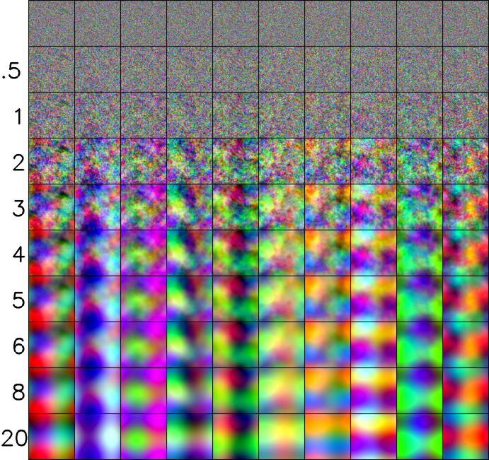
Figure 2: (left to right) 10 GFF images (each varying downwards) as a function of the power $\gamma$ of the index (mentioned on the left).

A GFF image can be obtained from a noise image in the following way:

1. First, sample an $n{\mkern-2.0mu\times\mkern-2.0mu}n$ noise image ${\mathbf{z}}$ from the standard complex normal distribution with covariance matrix $\Gamma={\mathbf{I}}_{N}$ where $N=n^{2}$ is the total number of pixels, and pseudo-covariance matrix $C={\bm{0}}$: ${\mathbf{z}}\sim{\mathcal{C}}{\mathcal{N}}({\bm{0}},{\mathbf{I}}_{N},{\bm{0}})$.

   The standard complex normal distribution is one where the real part ${\mathbf{x}}$ and imaginary part ${\mathbf{y}}$ are each distributed as the standard normal distribution with variance $\frac{1}{2}{\mathbf{I}}_{N}$. Let ${\bm{\Sigma}}_{{\mathbf{a}}{\mathbf{b}}}$ be the covariance matrix between ${\mathbf{a}}$ and ${\mathbf{b}}$. We know that ${\bm{\Sigma}}_{{\mathbf{x}}{\mathbf{x}}}={\bm{\Sigma}}_{{\mathbf{y}}{\mathbf{y}}}=\frac{1}{2}{\mathbf{I}}_{N}$, and ${\bm{\Sigma}}_{{\mathbf{x}}{\mathbf{y}}}={\bm{\Sigma}}_{{\mathbf{y}}{\mathbf{x}}}={\bm{0}}_{N}$ Then:

   $$\Gamma =\mathbb{E}_{\mathbf{z}}[{\mathbf{z}}{\mathbf{z}}^{H}]={\bm{\Sigma}}_{{\mathbf{x}}{\mathbf{x}}}+{\bm{\Sigma}}_{{\mathbf{y}}{\mathbf{y}}}+i({\bm{\Sigma}}_{{\mathbf{y}}{\mathbf{x}}}-{\bm{\Sigma}}_{{\mathbf{x}}{\mathbf{y}}})={\mathbf{I}}_{N}$$ (65)

   $$C =\mathbb{E}_{\mathbf{z}}[{\mathbf{z}}{\mathbf{z}}^{T}]={\bm{\Sigma}}_{{\mathbf{x}}{\mathbf{x}}}-{\bm{\Sigma}}_{{\mathbf{y}}{\mathbf{y}}}+i({\bm{\Sigma}}_{{\mathbf{y}}{\mathbf{x}}}+{\bm{\Sigma}}_{{\mathbf{x}}{\mathbf{y}}})={\bm{0}}_{N}$$ (66)

2. Apply the Discrete Fourier Transform using the $N{\mkern-2.0mu\times\mkern-2.0mu}N$ weights matrix ${\mathbf{W}}_{N}$: ${\mathbf{W}}_{N}{\mathbf{z}}$.

3. Consider a diagonal $N{\mkern-2.0mu\times\mkern-2.0mu}N$ matrix of the reciprocal of an index value $k_{ij}$ per pixel $(i,j)$ in Fourier space : ${\mathbf{K}}^{-1}=[1/|k_{ij}|]_{(i,j)}$, and multiply this with the above: ${\mathbf{K}}^{-1}{\mathbf{W}}_{N}{\mathbf{z}}$.

4. Take its Inverse Discrete Fourier Transform (${\mathbf{W}}_{N}^{-1}$) to make the raw GFF image: ${\mathbf{W}}_{N}^{-1}{\mathbf{K}}^{-1}{\mathbf{W}}_{N}{\mathbf{z}}$. However, this results in a GFF image with a small variance.

5. Normalize the image with the standard deviation $\sigma_{N}$ corresponding to its resolution $N$:

   $${\mathbf{g}} =\frac{1}{\sigma_{N}}{\mathbf{W}}_{N}^{-1}{\mathbf{K}}^{-1}{\mathbf{W}}_{N}{\mathbf{z}}\quad\iff\quad{\mathbf{z}}=\sigma_{N}{\mathbf{W}}_{N}^{-1}{\mathbf{K}}{\mathbf{W}}_{N}{\mathbf{g}}$$ (67)

6. Extract only the real part of ${\mathbf{g}}$, and normalize accordingly (refer Section C.2):

   $${\mathbf{g}}_{\text{real}} =\frac{1}{\sqrt{2N}\sigma_{N}}\text{Real}\left({\mathbf{W}}_{N}^{-1}{\mathbf{K}}^{-1}{\mathbf{W}}_{N}{\mathbf{z}}\right)\iff{\mathbf{z}}=\sqrt{2N}\sigma_{N}\text{Real}\left({\mathbf{W}}_{N}^{-1}{\mathbf{K}}{\mathbf{W}}_{N}{\mathbf{g}}_{\text{real}}\right)$$ (68)

C.1 Probability distribution of GFF

Let the probability distribution of GFF images be $\mathcal{G}$. This can be seen as a non-isotropic multivariate Gaussian with a non-diagonal covariance matrix ${\bm{\Sigma}}$:

$${\mathbf{g}}\sim{\mathcal{G}}={\mathcal{N}}({\bm{\mu}},{\bm{\Sigma}})={\mathcal{N}}({\bm{0}}_{N},{\bm{\Sigma}})$$ (69)

We know from the properties of Discrete Fourier Transform (following the normalization convention of the Pytorch / Numpy implementation) that:

$${\mathbf{W}}_{N}={\mathbf{W}}_{N}^{T};{\mathbf{W}}_{N}^{-1}={{\mathbf{W}}_{N}^{-1}}^{T};{\mathbf{W}}_{N}^{-1}=\frac{1}{N}{\mathbf{W}}_{N}^{*}=\frac{1}{N}{\mathbf{W}}_{N}^{H}$$ (70)

${\bm{\mu}}$ is given by:

$${\bm{\mu}} =\mathbb{E}_{{\mathbf{g}}}[{\mathbf{g}}]=\mathbb{E}_{\mathbf{z}}\left[\frac{1}{\sigma_{N}}{\mathbf{W}}_{N}^{-1}{\mathbf{K}}^{-1}{\mathbf{W}}_{N}{\mathbf{z}}\right]=\frac{1}{\sigma_{N}}{\mathbf{W}}_{N}^{-1}{\mathbf{K}}^{-1}{\mathbf{W}}_{N}\mathbb{E}_{\mathbf{z}}\left[{\mathbf{z}}\right]$$

$$\implies{\bm{\mu}} ={\bm{0}}_{N}\qquad[\because\mathbb{E}_{\mathbf{z}}[{\mathbf{z}}]={\bm{0}}_{N}]$$ (71)

${\bm{\Sigma}}$ is given by:

$${\bm{\Sigma}} =\mathbb{E}_{{\mathbf{g}}}[\ {\mathbf{g}}\ {\mathbf{g}}^{T}\ ]$$

$$=\mathbb{E}_{\mathbf{z}}\left[\frac{1}{\sigma_{N}}{\mathbf{W}}_{N}^{-1}{\mathbf{K}}^{-1}{\mathbf{W}}_{N}{\mathbf{z}}\ \left(\frac{1}{\sigma_{N}}{\mathbf{W}}_{N}^{-1}{\mathbf{K}}^{-1}{\mathbf{W}}_{N}{\mathbf{z}}\right)^{T}\right]$$

$$=\mathbb{E}_{\mathbf{z}}\left[\frac{1}{\sigma_{N}^{2}}{\mathbf{W}}_{N}^{-1}{\mathbf{K}}^{-1}{\mathbf{W}}_{N}{\mathbf{z}}\ {\mathbf{z}}^{T}{\mathbf{W}}_{N}^{T}{\mathbf{K}}^{-1}{\mathbf{W}}_{N}^{-T}\right]\quad\quad[\because{\mathbf{K}}^{-1}\text{ is diagonal }]$$

$$=\frac{1}{\sigma_{N}^{2}}{\mathbf{W}}_{N}^{-1}{\mathbf{K}}^{-1}{\mathbf{W}}_{N}\mathbb{E}_{\mathbf{z}}[{\mathbf{z}}{\mathbf{z}}^{T}]{\mathbf{W}}_{N}{\mathbf{K}}^{-1}{\mathbf{W}}_{N}^{-1}$$

$$=\frac{1}{\sigma_{N}^{2}}{\mathbf{W}}_{N}^{-1}{\mathbf{K}}^{-1}{\mathbf{W}}_{N}{\mathbf{W}}_{N}{\mathbf{K}}^{-1}{\mathbf{W}}_{N}^{-1}\qquad\qquad\qquad[\because\mathbb{E}_{\mathbf{z}}[{\mathbf{z}}{\mathbf{z}}^{T}]={\mathbf{I}}_{N}]$$

$$=\left(\frac{1}{\sigma_{N}}{\mathbf{W}}_{N}^{-1}{\mathbf{K}}^{-1}{\mathbf{W}}_{N}\right)\left(\frac{1}{\sigma_{N}}{\mathbf{W}}_{N}^{-1}{\mathbf{K}}^{-1}{\mathbf{W}}_{N}\right)^{T}\quad[\because({\mathbf{W}}_{N}^{-1}{\mathbf{K}}^{-1}{\mathbf{W}}_{N})^{T}={\mathbf{W}}_{N}{\mathbf{K}}^{-1}{\mathbf{W}}_{N}^{-1}]$$

$\sigma_{N}^{2}$ is such that the variance of each variable is 1, i.e. each diagonal element of ${\bm{\Sigma}}$ is 1. Thus,

$$\sigma_{N}^{2}=\mathrm{Var}[{\bm{\Sigma}}_{N}]\quad\text{where }{\bm{\Sigma}}_{N}={\mathbf{W}}_{N}^{-1}{\mathbf{K}}^{-1}{\mathbf{W}}_{N}{\mathbf{W}}_{N}{\mathbf{K}}^{-1}{\mathbf{W}}_{N}^{-1}$$ (72)

Hence,

$$\sqrt{{\bm{\Sigma}}} =\frac{1}{\sigma_{N}}{\mathbf{W}}_{N}^{-1}{\mathbf{K}}^{-1}{\mathbf{W}}_{N},$$ (73)

$${\bm{\Sigma}} =\sqrt{{\bm{\Sigma}}}\sqrt{{\bm{\Sigma}}}^{T},$$ (74)

$$\sqrt{{\bm{\Sigma}}^{-1}} =\sigma_{N}{\mathbf{W}}_{N}^{-1}{\mathbf{K}}{\mathbf{W}}_{N}$$ (75)

$${\bm{\Sigma}}^{-1} =\sqrt{{\bm{\Sigma}}^{-1}}^{T}\sqrt{{\bm{\Sigma}}^{-1}},$$ (76)

C.2 Derivation of GFF ${\bm{\Sigma}}$ for real ${\mathbf{g}}$ and complex ${\mathbf{z}}$

z is complex, g is real : ${\bm{\mu}}$ is given by:

$${\bm{\mu}} =\mathbb{E}_{{\mathbf{g}}}[{\mathbf{g}}]=\mathbb{E}_{\mathbf{g}}[\ \frac{1}{2\sigma_{N}}({\mathbf{g}}+{\mathbf{g}}^{*})\ ]=\frac{1}{2\sigma_{N}}\left(\mathbb{E}_{\mathbf{g}}[{\mathbf{g}}]+\mathbb{E}_{\mathbf{g}}[{\mathbf{g}}^{*}]\right)$$

$$=\frac{1}{2\sigma_{N}}\left(\mathbb{E}_{\mathbf{z}}[{\mathbf{W}}_{N}^{-1}{\mathbf{K}}^{-1}{\mathbf{z}}]+\mathbb{E}_{\mathbf{z}}[({\mathbf{W}}_{N}^{-1}{\mathbf{K}}^{-1}{\mathbf{z}})^{*}]\right)$$

$$=\frac{1}{2\sigma_{N}}\left({\mathbf{W}}_{N}^{-1}{\mathbf{K}}^{-1}\mathbb{E}_{\mathbf{z}}[{\mathbf{z}}]+{\mathbf{W}}_{N}^{-1*}{\mathbf{K}}^{-1}\mathbb{E}_{\mathbf{z}}[{\mathbf{z}}^{*}]\right)$$

$$\implies{\bm{\mu}} ={\bm{0}}_{N}\qquad\qquad[\because\mathbb{E}_{\mathbf{z}}[{\mathbf{z}}]=\mathbb{E}_{\mathbf{z}}[{\mathbf{z}}^{*}]={\bm{0}}_{N}]$$ (77)

z is complex, g is real : ${\bm{\Sigma}}$ is given by:

$${\bm{\Sigma}} =\mathbb{E}_{{\mathbf{g}}}[\ {\mathbf{g}}\ {\mathbf{g}}^{T}\ ]$$

$$=\mathbb{E}_{\mathbf{g}}[\ \frac{1}{2\sigma_{N}}({\mathbf{g}}+{\mathbf{g}}^{*})\ \frac{1}{2\sigma_{N}}({\mathbf{g}}+{\mathbf{g}}^{*})^{T}\ ]$$

$$=\frac{1}{4\sigma_{N}^{2}}\mathbb{E}_{\mathbf{g}}[\ ({\mathbf{g}}+{\mathbf{g}}^{*})\ ({\mathbf{g}}^{T}+{\mathbf{g}}^{H})\ ]$$

$$=\frac{1}{4\sigma_{N}^{2}}\mathbb{E}_{\mathbf{g}}[\ {\mathbf{g}}{\mathbf{g}}^{T}+{\mathbf{g}}{\mathbf{g}}^{H}+{\mathbf{g}}^{*}{\mathbf{g}}^{T}+{\mathbf{g}}^{*}{\mathbf{g}}^{H}\ ]$$

$$=\frac{1}{4\sigma_{N}^{2}}\left(\mathbb{E}_{\mathbf{g}}[{\mathbf{g}}{\mathbf{g}}^{T}]+\mathbb{E}_{\mathbf{g}}[{\mathbf{g}}{\mathbf{g}}^{H}]+\mathbb{E}_{\mathbf{g}}[{\mathbf{g}}^{*}{\mathbf{g}}^{T}]+\mathbb{E}_{\mathbf{g}}[{\mathbf{g}}^{*}{\mathbf{g}}^{H}]\right)$$

$$\mathbb{E}_{\mathbf{g}}[{\mathbf{g}}{\mathbf{g}}^{T}] =\mathbb{E}_{\mathbf{z}}[{\mathbf{W}}_{N}^{-1}{\mathbf{K}}^{-1}{\mathbf{z}}\ ({\mathbf{W}}_{N}^{-1}{\mathbf{K}}^{-1}{\mathbf{z}})^{T}]$$

$$=\mathbb{E}_{\mathbf{z}}[{\mathbf{W}}_{N}^{-1}{\mathbf{K}}^{-1}{\mathbf{z}}\ {\mathbf{z}}^{T}{\mathbf{K}}^{-1}{\mathbf{W}}_{N}^{-T}]\quad[\because{\mathbf{K}}^{-1}\text{ is diagonal }]$$

$$={\mathbf{W}}_{N}^{-1}{\mathbf{K}}^{-1}\mathbb{E}_{\mathbf{z}}[{\mathbf{z}}{\mathbf{z}}^{T}]{\mathbf{K}}^{-1}{\mathbf{W}}_{N}^{-T}$$

$$={\bm{0}}_{N}\qquad\qquad\qquad\qquad\qquad\qquad\quad[\because\mathbb{E}_{\mathbf{z}}[{\mathbf{z}}{\mathbf{z}}^{T}]={\bm{0}}_{N}\text{ (\lx@cref{creftype~refnum}{eq:psudocov_z})}]$$

$$\mathbb{E}_{\mathbf{g}}[{\mathbf{g}}{\mathbf{g}}^{H}] =\mathbb{E}_{\mathbf{z}}[{\mathbf{W}}_{N}^{-1}{\mathbf{K}}^{-1}{\mathbf{z}}\ ({\mathbf{W}}_{N}^{-1}{\mathbf{K}}^{-1}{\mathbf{z}})^{H}]$$

$$=\mathbb{E}_{\mathbf{z}}[{\mathbf{W}}_{N}^{-1}{\mathbf{K}}^{-1}{\mathbf{z}}\ {\mathbf{z}}^{H}{\mathbf{K}}^{-1}{\mathbf{W}}_{N}^{-H}]\quad[\because{\bm{K}}^{-1}\text{ is real diagonal }]$$

$$={\mathbf{W}}_{N}^{-1}{\mathbf{K}}^{-1}\mathbb{E}_{\mathbf{z}}[{\mathbf{z}}{\mathbf{z}}^{H}]{\mathbf{K}}^{-1}\frac{1}{N}{\mathbf{W}}_{N}\quad[\because{\mathbf{W}}_{N}^{-1}=\frac{1}{N}{\mathbf{W}}_{N}^{H}\text{ (\lx@cref{creftype~refnum}{eq:fourier})}]$$

$$=\frac{1}{N}{\mathbf{W}}_{N}^{-1}{\mathbf{K}}^{-1}{\mathbf{K}}^{-1}{\mathbf{W}}_{N}\qquad\qquad[\because\mathbb{E}_{\mathbf{z}}[{\mathbf{z}}{\mathbf{z}}^{H}]={\mathbf{I}}_{N}\text{ (\lx@cref{creftype~refnum}{eq:cov_z})}]$$

$$\mathbb{E}_{\mathbf{g}}[{\mathbf{g}}^{*}{\mathbf{g}}^{T}] =\mathbb{E}_{\mathbf{z}}[({\mathbf{W}}_{N}^{-1}{\mathbf{K}}^{-1}{\mathbf{z}})^{*}\ ({\mathbf{W}}_{N}^{-1}{\mathbf{K}}^{-1}{\mathbf{z}})^{T}]$$

$$=\mathbb{E}_{\mathbf{z}}[{\mathbf{W}}_{N}^{-1*}{\mathbf{K}}^{-1}{\mathbf{z}}^{*}\ {\mathbf{z}}^{T}{\mathbf{K}}^{-1}{\mathbf{W}}_{N}^{-1}]$$

$$=\frac{1}{N}{\mathbf{W}}_{N}{\mathbf{K}}^{-1}\mathbb{E}_{\mathbf{z}}[{\mathbf{z}}^{*}{\mathbf{z}}^{T}]{\mathbf{K}}^{-1}{\mathbf{W}}_{N}^{-1}\quad[\because{\mathbf{W}}_{N}^{-1}=\frac{1}{N}{\mathbf{W}}_{N}^{*}\text{ (\lx@cref{creftype~refnum}{eq:fourier})}]$$

$$=\frac{1}{N}{\mathbf{W}}_{N}{\mathbf{K}}^{-1}{\mathbf{K}}^{-1}{\mathbf{W}}_{N}^{-1}\quad[\because\mathbb{E}_{\mathbf{z}}[{\mathbf{z}}^{*}{\mathbf{z}}^{T}]=\mathbb{E}_{\mathbf{z}}[{\mathbf{z}}{\mathbf{z}}^{H}]^{*}={\mathbf{I}}_{N}\text{ (\lx@cref{creftype~refnum}{eq:cov_z})}]$$

$$\mathbb{E}_{\mathbf{g}}[{\mathbf{g}}^{*}{\mathbf{g}}^{H}] =\mathbb{E}_{\mathbf{z}}[({\mathbf{W}}_{N}^{-1}{\mathbf{K}}^{-1}{\mathbf{z}})^{*}\ ({\mathbf{W}}_{N}^{-1}{\mathbf{K}}^{-1}{\mathbf{z}})^{H}]$$

$$=\mathbb{E}_{\mathbf{z}}[{\mathbf{W}}_{N}^{-1*}{\mathbf{K}}^{-1}{\mathbf{z}}^{*}\ {\mathbf{z}}^{H}{\mathbf{K}}^{-1}{\mathbf{W}}_{N}^{-H}]$$

$$={\mathbf{W}}_{N}^{-1*}{\mathbf{K}}^{-1}\mathbb{E}_{\mathbf{z}}[{\mathbf{z}}^{*}{\mathbf{z}}^{H}]{\mathbf{K}}^{-1}{\mathbf{W}}_{N}^{-H}$$

$$={\bm{0}}_{N}\qquad\qquad\qquad\qquad[\because\mathbb{E}_{\mathbf{z}}[{\mathbf{z}}^{*}{\mathbf{z}}^{H}]=\mathbb{E}_{\mathbf{z}}[{\mathbf{z}}{\mathbf{z}}^{T}]^{*}={\bm{0}}_{N}\text{ (\lx@cref{creftype~refnum}{eq:cov_z})}]$$

$$\implies{\bm{\Sigma}} =\frac{1}{4\sigma_{N}^{2}}\left({\bm{0}}+\frac{1}{N}{\mathbf{W}}_{N}^{-1}{\mathbf{K}}^{-1}{\mathbf{K}}^{-1}{\mathbf{W}}_{N}+\frac{1}{N}{\mathbf{W}}_{N}{\mathbf{K}}^{-1}{\mathbf{K}}^{-1}{\mathbf{W}}_{N}^{-1}+{\bm{0}}\right)$$

$$=\frac{1}{4N\sigma_{N}^{2}}\left({\mathbf{W}}_{N}^{-1}{\mathbf{K}}^{-1}{\mathbf{K}}^{-1}{\mathbf{W}}_{N}+{\mathbf{W}}_{N}{\mathbf{K}}^{-1}{\mathbf{K}}^{-1}{\mathbf{W}}_{N}^{-1}\right)$$

$$=\frac{1}{4N\sigma_{N}^{2}}\left({\mathbf{W}}_{N}^{-1}{\mathbf{K}}^{-1}{\mathbf{K}}^{-1}{\mathbf{W}}_{N}+(N{\mathbf{W}}_{N}^{-1*}){\mathbf{K}}^{-1}{\mathbf{K}}^{-1}(\frac{1}{N}{\mathbf{W}}_{N}^{*})\right)$$

$$=\frac{1}{2N\sigma_{N}^{2}}\left(\frac{1}{2}\left({\mathbf{W}}_{N}^{-1}{\mathbf{K}}^{-1}{\mathbf{K}}^{-1}{\mathbf{W}}_{N}+({\mathbf{W}}_{N}^{-1}{\mathbf{K}}^{-1}{\mathbf{K}}^{-1}{\mathbf{W}}_{N})^{*}\right)\right)$$

$$\implies{\bm{\Sigma}} =\frac{1}{2N\sigma_{N}^{2}}\text{Real}\left({\mathbf{W}}_{N}^{-1}{\mathbf{K}}^{-1}{\mathbf{K}}^{-1}{\mathbf{W}}_{N}\right),$$ (78)

$$\sqrt{{\bm{\Sigma}}} =\frac{1}{\sqrt{2N}\sigma_{N}}\text{Real}\left({\mathbf{W}}_{N}^{-1}{\mathbf{K}}^{-1}{\mathbf{W}}_{N}\right),$$ (79)

$${\bm{\Sigma}}^{-1} =2N\sigma_{N}^{2}\text{Real}\left({\mathbf{W}}_{N}^{-1}{\mathbf{K}}{\mathbf{K}}{\mathbf{W}}_{N}\right),$$ (80)

$$\sqrt{{\bm{\Sigma}}^{-1}} =\sqrt{2N}\sigma_{N}\text{Real}\left({\mathbf{W}}_{N}^{-1}{\mathbf{K}}{\mathbf{W}}_{N}\right)$$ (81)

C.3 Log probability of transformation

$${\mathbf{g}} =\sqrt{{\bm{\Sigma}}}{\mathbf{z}}$$

$$\implies\log p({\mathbf{g}}) =\log p({\mathbf{z}})-\log\left|\det\frac{{\mathrm{d}}{\mathbf{g}}}{{\mathrm{d}}{\mathbf{z}}}\right|$$

$$=\log p({\mathbf{z}})-\log\left|\det\sqrt{{\bm{\Sigma}}}\right|$$

$$=\log p({\mathbf{z}})-\log\left|\det\frac{1}{\sqrt{2N}\sigma_{N}}\text{Real}\left({\mathbf{W}}_{N}^{-1}{\mathbf{K}}^{-1}{\mathbf{W}}_{N}\right)\right|$$

$$=\log p({\mathbf{z}})-\frac{1}{\sqrt{2N}\sigma_{N}}\log\left|\det{\mathbf{K}}^{-1}\right|$$

This is useful for building (normalizing) flows using non-isotropic Gaussian noise.

C.4 Varying ${\mathbf{K}}$

The index matrix ${\mathbf{K}}$ involves computation of an index value $k_{ij}$ per pixel $(i,j)$. However, this index value could be raised to any power $\gamma$ i.e. $|k_{ij}|^{\gamma}$. The effect of varying $\gamma$ can be seen in Figure 2 : greater the $\gamma$, the more correlated are neighbouring pixels.

Appendix D Score Matching Langevin Dynamics (SMLD) [16, 17]

D.1 Score for SMLD

For isotropic Gaussian noise as in SMLD,

$$q_{\sigma_{t}}^{\text{SMLD}}({\mathbf{x}}_{i}\mid{\mathbf{x}})={\mathcal{N}}({\mathbf{x}}_{i}\mid{\mathbf{x}},\sigma_{i}^{2}{\mathbf{I}})\implies{\mathbf{x}}_{i}={\mathbf{x}}+\sigma_{i}{\bm{\epsilon}}$$ (82)

$$\implies\nabla_{{\mathbf{x}}_{i}}\log q_{\sigma_{i}}^{\text{SMLD}}({\mathbf{x}}_{i}\mid{\mathbf{x}})=-\frac{1}{\sigma_{i}^{2}}({\mathbf{x}}_{i}-{\mathbf{x}})=-\frac{1}{\sigma_{i}}{\bm{\epsilon}}$$ (83)

D.2 Objective function for SMLD

The objective function for SMLD at noise level $\sigma$ is:

$$\ell^{\text{SMLD}}({\bm{\theta}};\sigma_{i})\triangleq\ \frac{1}{2}\mathbb{E}_{q_{\sigma_{i}}({\mathbf{x}}_{i}\mid{\mathbf{x}})p({\mathbf{x}})}\bigg{[}\left\|{\mathbf{s}}_{\bm{\theta}}({\mathbf{x}}_{i},\sigma_{i})+\frac{1}{\sigma_{i}^{2}}({\mathbf{x}}_{i}-{\mathbf{x}})\right\|_{2}^{2}\bigg{]}$$ (84)

D.3 Variance of actual score for SMLD

$$\mathbb{E}\left[\left\|\nabla_{{\mathbf{x}}_{i}}\log q_{\sigma_{i}}^{\text{SMLD}}({\mathbf{x}}_{i}\mid{\mathbf{x}})\right\|_{2}^{2}\right] =\mathbb{E}\left[\left\|-\frac{({\mathbf{x}}_{i}-{\mathbf{x}})}{\sigma_{i}^{2}}\right\|_{2}^{2}\right]=\mathbb{E}\left[\left\|\frac{\sigma_{i}{\bm{\epsilon}}}{\sigma_{i}^{2}}\right\|_{2}^{2}\right]=\frac{1}{\sigma_{i}^{2}}\mathbb{E}\left[\left\|{\bm{\epsilon}}\right\|_{2}^{2}\right]=\frac{1}{\sigma_{i}^{2}}$$ (85)

D.4 Overall objective function for SMLD

[16, 17] chose a geometric series of $\sigma_{i}$’s, i.e. $\sigma_{i-1}/\sigma_{i}=\gamma$. The overall objective function was a weighted combination of the objectives at different noise levels, the weight being $\lambda(\sigma_{i})=\sigma_{i}^{2}$:

$${\mathcal{L}}^{\text{SMLD}}({\bm{\theta}};\{\sigma_{i}\}_{i=1}^{L}) \triangleq\frac{1}{2L}\sum_{i=1}^{L}\mathbb{E}_{q_{\sigma_{i}}({\mathbf{x}}_{i}\mid{\mathbf{x}})p({\mathbf{x}})}\bigg{[}\left\|\sigma_{i}{\mathbf{s}}_{\bm{\theta}}({\mathbf{x}}_{i},\sigma_{i})+\frac{(\tilde{\mathbf{x}}-{\mathbf{x}})}{\sigma_{i}}\right\|_{2}^{2}\bigg{]}$$

$$=\frac{1}{2L}\sum_{i=1}^{L}\mathbb{E}_{q_{\sigma_{i}}({\mathbf{x}}_{i}\mid{\mathbf{x}})p({\mathbf{x}})}\bigg{[}\left\|\sigma_{i}{\mathbf{s}}_{\bm{\theta}}({\mathbf{x}}_{i},\sigma_{i})+{\bm{\epsilon}}\right\|_{2}^{2}\bigg{]}$$ (86)

D.5 Unconditional SMLD score estimation

Song et. al. discovered that empirically the estimated score was proportional to $\frac{1}{\sigma}$. So an unconditional score model is:

$${\mathbf{s}}_{\bm{\theta}}({\mathbf{x}}_{i},\sigma_{i})=-\frac{1}{\sigma_{i}}{\bm{\epsilon}}_{\bm{\theta}}({\mathbf{x}}_{i})$$ (87)

In this case, the overall objective function changes to:

$${\mathcal{L}}^{\text{SMLD}}({\bm{\theta}};\{\sigma_{i}\}_{i=1}^{L}) \triangleq\frac{1}{2L}\sum_{i=1}^{L}\mathbb{E}_{q_{\sigma_{i}}({\mathbf{x}}_{i}\mid{\mathbf{x}})p({\mathbf{x}})}\bigg{[}\left\|{\bm{\epsilon}}-{\bm{\epsilon}}_{\bm{\theta}}({\mathbf{x}}_{i})\right\|_{2}^{2}\bigg{]}$$ (88)

$$=\frac{1}{2L}\sum_{i=1}^{L}\mathbb{E}_{q_{\sigma_{i}}({\mathbf{x}}_{i}\mid{\mathbf{x}})p({\mathbf{x}})}\bigg{[}\left\|{\bm{\epsilon}}-{\bm{\epsilon}}_{\bm{\theta}}({\mathbf{x}}+\sigma_{i}{\bm{\epsilon}})\right\|_{2}^{2}\bigg{]}$$

D.6 Sampling in SMLD

$i=0$ corresponds to data, and $i=L$ corresponds to noise. Hence, $i=L,\cdots,0$ is the time order for sampling.

Using ALS from  [16, 17]:

$${\mathbf{x}}_{L}^{M}\sim{\mathcal{N}}({\mathbf{x}}\mid{\bm{0}},\sigma_{\max}{\mathbf{I}})$$

$$\begin{rcases}&{\mathbf{x}}_{i}^{M}={\mathbf{x}}_{i+1}^{0}\\ &\alpha_{i}={\epsilon}\sigma_{i}^{2}/\sigma_{\min}^{2}\\ &{\mathbf{x}}_{i}^{m-1}\leftarrow{\mathbf{x}}_{i}^{m}+\alpha_{i}{\mathbf{s}}_{{\bm{\theta}}^{*}}({\mathbf{x}}_{i}^{m},\sigma_{i})+\sqrt{2\alpha_{i}}{\bm{\epsilon}}_{i}^{m-1},m=M,\cdots,0\\ \implies&{\mathbf{x}}_{i}^{m-1}\leftarrow{\mathbf{x}}_{i}^{m}-\frac{\alpha_{i}}{\sigma_{i}}{\bm{\epsilon}}_{{\bm{\theta}}^{*}}({\mathbf{x}}_{i}^{m})+\sqrt{2\alpha_{i}}{\bm{\epsilon}}_{i}^{m-1},m=M,\cdots,0\end{rcases}i=L,\cdots,1$$ (89)

Using Consistent Annealed Sampling [8]:

$$\alpha_{i}={\epsilon}\sigma_{i}^{2}/\sigma_{\min}^{2}=\eta\sigma_{i}^{2};\ \beta=\sqrt{1-\gamma^{2}(1-{\epsilon}/\sigma_{\min}^{2})^{2}};\ \gamma=\sigma_{i}/\sigma_{i-1};\sigma_{i}>\sigma_{i-1}$$

$${\mathbf{x}}_{i-1}\leftarrow{\mathbf{x}}_{i}+\alpha_{i}{\mathbf{s}}_{{\bm{\theta}}^{*}}({\mathbf{x}}_{i},\sigma_{i})+\beta\sigma_{i-1}{\bm{\epsilon}}_{i-1},i=L,\cdots,1$$

$$\implies {\mathbf{x}}_{i-1}\leftarrow{\mathbf{x}}_{i}-\eta\sigma_{i}{\bm{\epsilon}}_{{\bm{\theta}}^{*}}({\mathbf{x}}_{i})+\beta\sigma_{i-1}{\bm{\epsilon}}_{i-1},i=L,\cdots,1$$ (90)

D.7 Expected Denoised Sample

From [13], assuming isotropic Gaussian noise, we know that the expected denoised sample ${\mathbf{x}}^{*}({\mathbf{x}}_{i},\sigma_{i})\triangleq\mathbb{E}_{{\mathbf{x}}\sim q_{\sigma_{i}}({\mathbf{x}}\mid{\mathbf{x}}_{i})}[{\mathbf{x}}]$ and the optimal score ${\mathbf{s}}_{{\bm{\theta}}^{*}}({\mathbf{x}}_{i},\sigma_{i})$ are related as:

$${\mathbf{s}}_{{\bm{\theta}}^{*}}({\mathbf{x}}_{i},\sigma_{i})=\frac{1}{\sigma_{i}^{2}}({\mathbf{x}}^{*}({\mathbf{x}}_{i},\sigma_{i})-{\mathbf{x}}_{i})$$

$$\implies {\mathbf{x}}^{*}({\mathbf{x}}_{i},\sigma_{i})={\mathbf{x}}_{i}+\sigma_{i}^{2}{\mathbf{s}}_{{\bm{\theta}}^{*}}({\mathbf{x}}_{i},\sigma_{i})={\mathbf{x}}_{i}-\sigma_{i}{\bm{\epsilon}}_{{\bm{\theta}}^{*}}({\mathbf{x}}_{i})$$ (91)

D.8 SDE formulation : Variance Exploding (VE) SDE

Forward process:

$${\mathbf{x}}_{i} ={\mathbf{x}}_{i-1}+\sqrt{\sigma_{i}^{2}-\sigma_{i-1}^{2}}{\bm{\epsilon}}_{i-1}$$

$$\implies{\mathbf{x}}(t+\Delta t) ={\mathbf{x}}(t)+\sqrt{(\sigma^{2}(t+\Delta t)-\sigma^{2}(t))\Delta t}\ {\bm{\epsilon}}(t)$$

$$\approx{\mathbf{x}}(t)+\sqrt{\frac{{\mathrm{d}}[\sigma^{2}(t)]}{{\mathrm{d}}t}\Delta t}\ {\mathbf{w}}(t)$$

$$\implies{\mathrm{d}}{\mathbf{x}} =\sqrt{\frac{{\mathrm{d}}[\sigma^{2}(t)]}{{\mathrm{d}}t}}\ {\mathrm{d}}{\mathbf{w}}$$ (92)

$${\mathrm{d}}{\mathbf{x}}={\mathbf{f}}({\mathbf{x}},t){\mathrm{d}}t+{\mathbf{L}}({\mathbf{x}},t){\mathrm{d}}{\mathbf{w}}\implies\frac{{\mathrm{d}}{\bm{\mu}}}{{\mathrm{d}}t}=\mathbb{E}_{\mathbf{x}}[{\mathbf{f}}({\mathbf{x}},t)],$$

$$\frac{{\mathrm{d}}\textbf{Cov}[{\mathbf{x}}]}{{\mathrm{d}}t}=\mathbb{E}_{\mathbf{x}}[{\mathbf{f}}({\mathbf{x}},t)({\mathbf{x}}-{\bm{\mu}})^{T}]+\mathbb{E}_{\mathbf{x}}[({\mathbf{x}}-{\bm{\mu}}){\mathbf{f}}({\mathbf{x}},t)^{T}]+\mathbb{E}_{\mathbf{x}}[{\mathbf{L}}({\mathbf{x}},t){\mathbf{Q}}{\mathbf{L}}^{T}({\mathbf{x}},t)]$$

where ${\mathbf{w}}$ is Brownian motion, ${\mathbf{Q}}$ is the PSD of ${\mathbf{w}}$. For GFF noise, ${\mathbf{Q}}={\bm{\Sigma}}$.

Mean and Covariance:

$$\frac{{\mathrm{d}}{\bm{\mu}}_{\text{SMLD}}(t)}{{\mathrm{d}}t}={\bm{0}}\implies{\bm{\mu}}_{\text{SMLD}}(t)={\bm{\mu}}(0)$$

$$\frac{{\mathrm{d}}{\bm{\Sigma}}_{\text{SMLD}}(t)}{{\mathrm{d}}t}=\mathbb{E}_{\mathbf{x}}\left[\sqrt{\frac{{\mathrm{d}}[\sigma^{2}(t)]}{{\mathrm{d}}t}}\sqrt{\frac{{\mathrm{d}}[\sigma^{2}(t)]}{{\mathrm{d}}t}}\right]=\frac{{\mathrm{d}}[\sigma^{2}(t)]}{{\mathrm{d}}t}$$

Appendix E Non-isotropic SMLD (NI-SMLD)

E.1 Score for NI-SMLD

$$q_{\sigma_{i}}^{\text{SMLD}}({\mathbf{x}}_{i}\mid{\mathbf{x}})={\mathcal{N}}({\mathbf{x}}_{i}\mid{\mathbf{x}},\sigma_{i}^{2}{\bm{\Sigma}})\implies{\mathbf{x}}_{i}={\mathbf{x}}+\sigma_{i}\sqrt{{\bm{\Sigma}}}{\bm{\epsilon}}\implies{\bm{\epsilon}}=\sqrt{{\bm{\Sigma}}^{-1}}\frac{{\mathbf{x}}_{i}-{\mathbf{x}}}{\sigma_{i}}$$ (93)

$$\implies\nabla_{{\mathbf{x}}_{i}}\log q_{\sigma_{i}}^{\text{SMLD}}({\mathbf{x}}_{i}\mid{\mathbf{x}})=-{\bm{\Sigma}}^{-1}\frac{{\mathbf{x}}_{i}-{\mathbf{x}}}{\sigma_{i}^{2}}=-\sqrt{{\bm{\Sigma}}^{-1}}\frac{{\bm{\epsilon}}}{\sigma_{i}}$$ (94)

E.2 Objective function for NI-SMLD

The objective function for SMLD at noise level $\sigma$ is:

$$\ell^{\text{NI}-\text{SMLD}}({\bm{\theta}};\sigma_{i}) \triangleq\ \frac{1}{2}\mathbb{E}_{q_{\sigma_{i}}({\mathbf{x}}_{i}\mid{\mathbf{x}})p({\mathbf{x}})}\bigg{[}\left\|{\mathbf{s}}_{\bm{\theta}}({\mathbf{x}}_{i},\sigma_{i})+{\bm{\Sigma}}^{-1}\frac{{\mathbf{x}}_{i}-{\mathbf{x}}}{\sigma_{i}^{2}}\right\|_{2}^{2}\bigg{]}$$ (95)

$$=\ \frac{1}{2}\mathbb{E}_{q_{\sigma_{i}}({\mathbf{x}}_{i}\mid{\mathbf{x}})p({\mathbf{x}})}\bigg{[}\left\|{\mathbf{s}}_{\bm{\theta}}({\mathbf{x}}_{i},\sigma_{i})+\frac{1}{\sigma_{i}}\sqrt{{\bm{\Sigma}}^{-1}}{\bm{\epsilon}}\right\|_{2}^{2}\bigg{]}$$ (96)

E.3 Expected value of score for NI-SMLD

$$\mathbb{E}\left[\left\|\nabla_{{\mathbf{x}}_{i}}\log q_{\sigma_{i}}^{\text{NI}-\text{SMLD}}({\mathbf{x}}_{i}\mid{\mathbf{x}})\right\|_{2}^{2}\right]=\mathbb{E}\left[\left\|-{\bm{\Sigma}}^{-1}\frac{{\mathbf{x}}_{i}-{\mathbf{x}}}{\sigma_{i}^{2}}\right\|_{2}^{2}\right]$$

$$=\mathbb{E}\left[\left\|{\bm{\Sigma}}^{-1}\frac{\sigma_{i}\sqrt{{\bm{\Sigma}}}{\bm{\epsilon}}}{\sigma_{i}^{2}}\right\|_{2}^{2}\right]=\frac{1}{\sigma_{i}^{2}}{\bm{\Sigma}}^{-1}\mathbb{E}\left[\left\|{\bm{\epsilon}}\right\|_{2}^{2}\right]=\frac{1}{\sigma_{i}^{2}}{\bm{\Sigma}}^{-1}\dim({\bm{\epsilon}})$$ (97)

E.4 Overall objective function for NI-SMLD

$\implies\lambda(\sigma_{i})=\sigma_{i}^{2}{\bm{\Sigma}}$

$${\mathcal{L}}^{\text{NI}-\text{SMLD}}({\bm{\theta}};\{\sigma_{i}\}_{i=1}^{L}) \triangleq\frac{1}{2L}\sum_{i=1}^{L}\mathbb{E}_{q_{\sigma_{i}}({\mathbf{x}}_{i}\mid{\mathbf{x}})p({\mathbf{x}})}\bigg{[}\left\|\sigma_{i}\sqrt{{\bm{\Sigma}}}{\mathbf{s}}_{\bm{\theta}}({\mathbf{x}}_{i},\sigma_{i})+\sqrt{{\bm{\Sigma}}^{-1}}\frac{(\tilde{\mathbf{x}}-{\mathbf{x}})}{\sigma_{i}}\right\|_{2}^{2}\bigg{]}$$

$$=\frac{1}{2L}\sum_{i=1}^{L}\mathbb{E}_{q_{\sigma_{i}}({\mathbf{x}}_{i}\mid{\mathbf{x}})p({\mathbf{x}})}\bigg{[}\left\|\sigma_{i}\sqrt{{\bm{\Sigma}}}{\mathbf{s}}_{\bm{\theta}}({\mathbf{x}}_{i},\sigma_{i})+{\bm{\epsilon}}\right\|_{2}^{2}\bigg{]}$$ (98)

E.5 Unconditional NI-SMLD score estimation

An unconditional score model is:

$${\mathbf{s}}_{\bm{\theta}}({\mathbf{x}}_{i},\sigma_{i})=-\sqrt{{\bm{\Sigma}}^{-1}}\frac{1}{\sigma_{i}}{\bm{\epsilon}}_{\bm{\theta}}({\mathbf{x}}_{i})$$ (99)

In this case, the overall objective function changes to:

$${\mathcal{L}}^{\text{GFF}-\text{SMLD}}({\bm{\theta}};\{\sigma_{i}\}_{i=1}^{L}) \triangleq\frac{1}{2L}\sum_{i=1}^{L}\mathbb{E}_{q_{\sigma_{i}}({\mathbf{x}}_{i}\mid{\mathbf{x}})p({\mathbf{x}})}\bigg{[}\left\|{\bm{\epsilon}}-{\bm{\epsilon}}_{\bm{\theta}}({\mathbf{x}}_{i})\right\|_{2}^{2}\bigg{]}$$

$$=\frac{1}{2L}\sum_{i=1}^{L}\mathbb{E}_{q_{\sigma_{i}}({\mathbf{x}}_{i}\mid{\mathbf{x}})p({\mathbf{x}})}\bigg{[}\left\|{\bm{\epsilon}}-{\bm{\epsilon}}_{\bm{\theta}}({\mathbf{x}}+\sigma_{i}\sqrt{{\bm{\Sigma}}}{\bm{\epsilon}})\right\|_{2}^{2}\bigg{]}$$ (100)

E.6 Sampling in NI-SMLD

$i=0$ corresponds to data, and $i=L$ corresponds to noise. Hence, $i=L,\cdots,0$ is the time order for sampling.

Forward : ${\mathbf{x}}_{i}={\mathbf{x}}_{i-1}+\sqrt{\sigma_{i}^{2}-\sigma_{i-1}^{2}}\sqrt{{\bm{\Sigma}}}{\bm{\epsilon}}_{i-1}$

Reverse:

From Song et. al., ALS:

$${\mathbf{x}}_{L}^{0}\sim{\mathcal{N}}({\mathbf{x}}\mid{\bm{0}},\sigma_{\max}\sqrt{{\bm{\Sigma}}})$$

$$\begin{rcases}&{\mathbf{x}}_{i}^{0}={\mathbf{x}}_{i+1}^{M}\\ &{\mathbf{x}}_{i}^{m+1}\leftarrow{\mathbf{x}}_{i}^{m}+\alpha_{i}{\mathbf{s}}_{{\bm{\theta}}^{*}}({\mathbf{x}}_{i}^{m},\sigma_{i})+\sqrt{2\alpha_{i}}\sqrt{{\bm{\Sigma}}}{\bm{\epsilon}}_{i}^{m+1},m=1,\cdots,M\end{rcases}i=L,\cdots,1$$ (101)

$$\alpha_{i}={\epsilon}\sigma_{i}^{2}/\sigma_{L}^{2}$$

From Alexia et. al., CAS:

$${\mathbf{x}}_{i-1}\leftarrow{\mathbf{x}}_{i}+\alpha_{i}{\mathbf{s}}_{{\bm{\theta}}^{*}}({\mathbf{x}}_{i},\sigma_{i})+\beta\sigma_{i-1}\sqrt{{\bm{\Sigma}}}{\bm{\epsilon}}_{i-1},i=L,\cdots,1$$ (102)

$$\alpha_{i}={\epsilon}\sigma_{t}^{2}/\sigma_{\min}^{2};\ \beta=\sqrt{1-\gamma^{2}(1-{\epsilon}/\sigma_{\min}^{2})^{2}};\ \gamma=\sigma_{t}/\sigma_{t-1};\sigma_{t}>\sigma_{t-1}$$

E.7 Expected Denoised Sample

From [13], assuming isotropic Gaussian noise of covariance $\sigma^{2}{\bm{\Sigma}}$, we know that the expected denoised sample ${\mathbf{x}}^{*}(\tilde{\mathbf{x}},\sigma)\triangleq\mathbb{E}_{{\mathbf{x}}\sim q_{\sigma}({\mathbf{x}}\mid\tilde{\mathbf{x}})}[{\mathbf{x}}]$ and the optimal score ${\mathbf{s}}_{{\bm{\theta}}^{*}}(\tilde{\mathbf{x}},\sigma)$ are related as:

$${\mathbf{s}}_{{\bm{\theta}}^{*}}(\tilde{\mathbf{x}},\sigma)=\frac{1}{\sigma^{2}}{\bm{\Sigma}}^{-1}({\mathbf{x}}^{*}(\tilde{\mathbf{x}},\sigma)-\tilde{\mathbf{x}})$$

$$\implies {\mathbf{x}}^{*}(\tilde{\mathbf{x}},\sigma)=\tilde{\mathbf{x}}+\sigma^{2}{\bm{\Sigma}}\ {\mathbf{s}}_{{\bm{\theta}}^{*}}(\tilde{\mathbf{x}},\sigma)=\tilde{\mathbf{x}}-\sigma\sqrt{{\bm{\Sigma}}}\ {\bm{\epsilon}}_{{\bm{\theta}}^{*}}(\tilde{\mathbf{x}})$$ (103)

E.8 Initial noise scale for NI-SMLD

Let $\hat{p}_{\sigma_{1}}({\mathbf{x}})\triangleq\frac{1}{N}\sum_{i=1}^{N}p^{(i)}({\mathbf{x}})$, where $p^{(i)}({\mathbf{x}})\triangleq{\mathcal{N}}({\mathbf{x}}\mid{\mathbf{x}}^{(i)},\sigma_{1}^{2}{\bm{\Sigma}})$. With $r^{(i)}({\mathbf{x}})\triangleq\frac{p^{(i)}({\mathbf{x}})}{\sum_{k=1}^{N}p^{(k)}({\mathbf{x}})}$, the score function is $\nabla_{\mathbf{x}}\log\hat{p}_{\sigma_{1}}({\mathbf{x}})=\sum_{i=1}^{N}r^{(i)}({\mathbf{x}})\nabla_{\mathbf{x}}\log p^{(i)}({\mathbf{x}})$.

We know that:

$${\mathcal{N}}({\mathbf{x}}\mid{\mathbf{x}}^{(i)},\sigma_{1}^{2}{\bm{\Sigma}})=\frac{1}{(2\pi)^{D/2}\sigma_{1}^{D}|{\bm{\Sigma}}|^{1/2}}\exp\left(-\frac{1}{2\sigma_{1}^{2}}({\mathbf{x}}-{\mathbf{x}}^{(i)})^{T}{\bm{\Sigma}}^{-1}({\mathbf{x}}-{\mathbf{x}}^{(i)})\right)$$

$$\mathbb{E}_{p^{(i)}({\mathbf{x}})}[r^{(j)}({\mathbf{x}})]=\int\frac{p^{(i)}({\mathbf{x}})p^{(j)}({\mathbf{x}})}{\sum_{k=1}^{N}p^{(k)}({\mathbf{x}})}\mathrm{d}{\mathbf{x}}\leq\int\frac{p^{(i)}({\mathbf{x}})p^{(j)}({\mathbf{x}})}{p^{(i)}({\mathbf{x}})+p^{(j)}({\mathbf{x}})}\mathrm{d}{\mathbf{x}}$$

$$=\frac{1}{2}\int\frac{2}{\frac{1}{p^{(i)}({\mathbf{x}})}+\frac{1}{p^{(j)}({\mathbf{x}})}}\mathrm{d}{\mathbf{x}}\leq\frac{1}{2}\int\sqrt{p^{(i)}({\mathbf{x}})p^{(j)}({\mathbf{x}})}\mathrm{d}{\mathbf{x}}$$

$$=\frac{1}{2}\frac{1}{(2\pi)^{D/2}\sigma_{1}^{D}|{\bm{\Sigma}}|^{1/2}}\int\exp\bigg{(}-\frac{1}{4\sigma_{1}^{2}}\bigg{(}({\mathbf{x}}-{\mathbf{x}}^{(i)})^{T}{\bm{\Sigma}}^{-1}({\mathbf{x}}-{\mathbf{x}}^{(i)})+({\mathbf{x}}-{\mathbf{x}}^{(j)})^{T}{\bm{\Sigma}}^{-1}({\mathbf{x}}-{\mathbf{x}}^{(j)})\bigg{)}\mathrm{d}{\mathbf{x}}$$

$$=\frac{1}{2}\frac{1}{(2\pi)^{D/2}\sigma_{1}^{D}|{\bm{\Sigma}}|^{1/2}}\int\exp\bigg{(}-\frac{1}{4\sigma_{1}^{2}}\bigg{(}({\mathbf{x}}-{\mathbf{x}}^{(i)})^{T}{\bm{\Sigma}}^{-1}({\mathbf{x}}-{\mathbf{x}}^{(i)})+({\mathbf{x}}-{\mathbf{x}}^{(j)})^{T}{\bm{\Sigma}}^{-1}({\mathbf{x}}-{\mathbf{x}}^{(i)}+{\mathbf{x}}^{(i)}-{\mathbf{x}}^{(j)})\bigg{)}\mathrm{d}{\mathbf{x}}$$

$$=\frac{1}{2}\frac{1}{(2\pi)^{D/2}\sigma_{1}^{D}|{\bm{\Sigma}}|^{1/2}}\int\exp\bigg{(}-\frac{1}{4\sigma_{1}^{2}}\bigg{(}({\mathbf{x}}-{\mathbf{x}}^{(i)})^{T}{\bm{\Sigma}}^{-1}({\mathbf{x}}-{\mathbf{x}}^{(i)})+({\mathbf{x}}-{\mathbf{x}}^{(j)})^{T}{\bm{\Sigma}}^{-1}({\mathbf{x}}-{\mathbf{x}}^{(i)})$$

$$\qquad\qquad\qquad\qquad\qquad\qquad\qquad+({\mathbf{x}}-{\mathbf{x}}^{(j)})^{T}{\bm{\Sigma}}^{-1}({\mathbf{x}}^{(i)}-{\mathbf{x}}^{(j)})\bigg{)}\mathrm{d}{\mathbf{x}}$$

$$=\frac{1}{2}\frac{1}{(2\pi)^{D/2}\sigma_{1}^{D}|{\bm{\Sigma}}|^{1/2}}\int\exp\bigg{(}-\frac{1}{4\sigma_{1}^{2}}\bigg{(}({\mathbf{x}}-{\mathbf{x}}^{(i)})^{T}{\bm{\Sigma}}^{-1}({\mathbf{x}}-{\mathbf{x}}^{(i)})+({\mathbf{x}}-{\mathbf{x}}^{(i)}+{\mathbf{x}}^{(i)}-{\mathbf{x}}^{(j)})^{T}{\bm{\Sigma}}^{-1}({\mathbf{x}}-{\mathbf{x}}^{(i)})$$

$$\qquad\qquad\qquad\qquad\qquad\qquad\qquad+({\mathbf{x}}-{\mathbf{x}}^{(i)}+{\mathbf{x}}^{(i)}-{\mathbf{x}}^{(j)})^{T}{\bm{\Sigma}}^{-1}({\mathbf{x}}^{(i)}-{\mathbf{x}}^{(j)})\bigg{)}\mathrm{d}{\mathbf{x}}$$

$$=\frac{1}{2}\frac{1}{(2\pi)^{D/2}\sigma_{1}^{D}|{\bm{\Sigma}}|^{1/2}}\int\exp\bigg{(}-\frac{1}{4\sigma_{1}^{2}}\bigg{(}({\mathbf{x}}-{\mathbf{x}}^{(i)})^{T}{\bm{\Sigma}}^{-1}({\mathbf{x}}-{\mathbf{x}}^{(i)})+({\mathbf{x}}-{\mathbf{x}}^{(i)})^{T}{\bm{\Sigma}}^{-1}({\mathbf{x}}-{\mathbf{x}}^{(i)})$$

$$\qquad\qquad\qquad\qquad\qquad\qquad\qquad+({\mathbf{x}}^{(i)}-{\mathbf{x}}^{(j)})^{T}{\bm{\Sigma}}^{-1}({\mathbf{x}}-{\mathbf{x}}^{(i)})+({\mathbf{x}}-{\mathbf{x}}^{(i)})^{T}{\bm{\Sigma}}^{-1}({\mathbf{x}}^{(i)}-{\mathbf{x}}^{(j)})$$

$$\qquad\qquad\qquad\qquad\qquad\qquad\qquad+({\mathbf{x}}^{(i)}-{\mathbf{x}}^{(j)})^{T}{\bm{\Sigma}}^{-1}({\mathbf{x}}^{(i)}-{\mathbf{x}}^{(j)})\bigg{)}\mathrm{d}{\mathbf{x}}$$

$$=\frac{1}{2}\frac{1}{(2\pi)^{D/2}\sigma_{1}^{D}|{\bm{\Sigma}}|^{1/2}}\int\exp\bigg{(}-\frac{1}{2\sigma_{1}^{2}}\bigg{(}({\mathbf{x}}-{\mathbf{x}}^{(i)})^{T}{\bm{\Sigma}}^{-1}({\mathbf{x}}-{\mathbf{x}}^{(i)})$$

$$\qquad\qquad\qquad\qquad\qquad\qquad\qquad+({\mathbf{x}}-{\mathbf{x}}^{(i)})^{T}{\bm{\Sigma}}^{-1}({\mathbf{x}}^{(i)}-{\mathbf{x}}^{(j)})$$

$$\qquad\qquad\qquad\qquad\qquad\qquad\qquad+\frac{1}{2}({\mathbf{x}}^{(i)}-{\mathbf{x}}^{(j)})^{T}{\bm{\Sigma}}^{-1}({\mathbf{x}}^{(i)}-{\mathbf{x}}^{(j)})\bigg{)}\mathrm{d}{\mathbf{x}}$$

$$=\frac{1}{2}\frac{1}{(2\pi)^{D/2}\sigma_{1}^{D}|{\bm{\Sigma}}|^{1/2}}\int\exp\bigg{(}-\frac{1}{2\sigma_{1}^{2}}\bigg{(}({\mathbf{x}}-{\mathbf{x}}^{(i)})^{T}{\bm{\Sigma}}^{-1}({\mathbf{x}}-{\mathbf{x}}^{(i)})$$

$$\qquad\qquad\qquad\qquad\qquad\qquad\qquad+2({\mathbf{x}}-{\mathbf{x}}^{(i)})^{T}{\bm{\Sigma}}^{-1}\frac{({\mathbf{x}}^{(i)}-{\mathbf{x}}^{(j)})}{2}$$

$$\qquad\qquad\qquad\qquad\qquad\qquad\qquad+\frac{({\mathbf{x}}^{(i)}-{\mathbf{x}}^{(j)})}{2}^{T}{\bm{\Sigma}}^{-1}\frac{({\mathbf{x}}^{(i)}-{\mathbf{x}}^{(j)})}{2}-\frac{({\mathbf{x}}^{(i)}-{\mathbf{x}}^{(j)})}{2}^{T}{\bm{\Sigma}}^{-1}\frac{({\mathbf{x}}^{(i)}-{\mathbf{x}}^{(j)})}{2}$$

$$\qquad\qquad\qquad\qquad\qquad\qquad\qquad+\frac{1}{2}({\mathbf{x}}^{(i)}-{\mathbf{x}}^{(j)})^{T}{\bm{\Sigma}}^{-1}({\mathbf{x}}^{(i)}-{\mathbf{x}}^{(j)})\bigg{)}\mathrm{d}{\mathbf{x}}$$

$$=\frac{1}{2}\frac{1}{(2\pi)^{D/2}\sigma_{1}^{D}|{\bm{\Sigma}}|^{1/2}}\int\exp\bigg{(}-\frac{1}{2\sigma_{1}^{2}}\bigg{(}({\mathbf{x}}-{\mathbf{x}}^{(i)}+\frac{({\mathbf{x}}^{(i)}-{\mathbf{x}}^{(j)})}{2})^{T}{\bm{\Sigma}}^{-1}({\mathbf{x}}-{\mathbf{x}}^{(i)}+\frac{({\mathbf{x}}^{(i)}-{\mathbf{x}}^{(j)})}{2})$$

$$\qquad\qquad\qquad\qquad\qquad\qquad\qquad+\frac{1}{4}({\mathbf{x}}^{(i)}-{\mathbf{x}}^{(j)})^{T}{\bm{\Sigma}}^{-1}({\mathbf{x}}^{(i)}-{\mathbf{x}}^{(j)})\bigg{)}\mathrm{d}{\mathbf{x}}$$

$$=\frac{1}{2}\exp\bigg{(}-\frac{1}{8\sigma_{1}^{2}}({\mathbf{x}}^{(i)}-{\mathbf{x}}^{(j)})^{T}{\bm{\Sigma}}^{-1}({\mathbf{x}}^{(i)}-{\mathbf{x}}^{(j)})\bigg{)}$$

$$\qquad\qquad\int\frac{1}{(2\pi)^{D/2}\sigma_{1}^{D}|{\bm{\Sigma}}|^{1/2}}\exp\bigg{(}-\frac{1}{2\sigma_{1}^{2}}\bigg{(}({\mathbf{x}}-\frac{({\mathbf{x}}^{(i)}+{\mathbf{x}}^{(j)})}{2})^{T}{\bm{\Sigma}}^{-1}({\mathbf{x}}-\frac{({\mathbf{x}}^{(i)}+{\mathbf{x}}^{(j)})}{2})\bigg{)}\mathrm{d}{\mathbf{x}}$$

$$=\frac{1}{2}\exp\bigg{(}-\frac{1}{8\sigma_{1}^{2}}({\mathbf{x}}^{(i)}-{\mathbf{x}}^{(j)})^{T}{\bm{\Sigma}}^{-1}({\mathbf{x}}^{(i)}-{\mathbf{x}}^{(j)})\bigg{)}$$

$$\implies\frac{1}{\sigma_{1}^{2}}({\mathbf{x}}^{(i)}-{\mathbf{x}}^{(j)})^{T}{\bm{\Sigma}}^{-1}({\mathbf{x}}^{(i)}-{\mathbf{x}}^{(j)})\approx 1$$

$$\implies(\sqrt{{\bm{\Sigma}}^{-1}}({\mathbf{x}}^{(i)}-{\mathbf{x}}^{(j)}))^{T}(\sqrt{{\bm{\Sigma}}^{-1}}({\mathbf{x}}^{(i)}-{\mathbf{x}}^{(j)}))\approx\sigma_{1}^{2}$$

$$\implies\left\|\sqrt{{\bm{\Sigma}}^{-1}}({\mathbf{x}}^{(i)}-{\mathbf{x}}^{(j)})\right\|_{2}\approx\sigma_{1}$$

$$\implies\left\|\sigma_{N}\ \text{Real}\big{(}{\mathbf{W}}_{N}^{-1}{\mathbf{K}}{\mathbf{W}}_{N}({\mathbf{x}}^{(i)}-{\mathbf{x}}^{(j)})\big{)}\right\|_{2}\approx\sigma_{1}$$

$$\implies\left\|\sigma_{N}{\mathbf{W}}_{N}^{-1}{\mathbf{K}}{\mathbf{W}}_{N}{\mathbf{x}}^{(i)}-\sigma_{N}{\mathbf{W}}_{N}^{-1}{\mathbf{K}}{\mathbf{W}}_{N}{\mathbf{x}}^{(j)}\right\|_{2}\approx\sigma_{1}$$

For CIFAR10, this $\sigma_{1}\approx 20$ for NI-SMLD (whereas for SMLD $\sigma_{1}\approx 50$).

E.9 Other noise scales

$$p_{\sigma_{i}}(r) ={\mathcal{N}}(r\mid m_{i},s_{i}^{2}),\text{where }m_{i}\triangleq\sqrt{D}\sigma_{i};s_{i}^{2}\triangleq\sigma_{i}^{2}/2$$

$${\mathcal{I}}_{i} \triangleq(m_{i}-3s_{i},m_{i}+3s_{i})$$

$$p_{\sigma_{i}}(r\in{\mathcal{I}}_{i-1}) =\Phi\left(\frac{(m_{i-1}+3s_{i-1})-m_{i}}{s_{i}}\right)-\Phi\left(\frac{(m_{i-1}-3s_{i-1})-m_{i}}{s_{i}}\right)$$

$$=\Phi\left(\frac{\sqrt{2}}{\sigma_{i}}(\sqrt{D}\sigma_{i-1}+\frac{3\sigma_{i-1}}{\sqrt{2}}-\sqrt{D}\sigma_{i})\right)-\Phi\left(\frac{\sqrt{2}}{\sigma_{i}}(\sqrt{D}\sigma_{i-1}-\frac{3\sigma_{i-1}}{\sqrt{2}}-\sqrt{D}\sigma_{i})\right)$$

$$=\Phi\left(\frac{1}{\sigma_{i}}(\sqrt{2D}(\sigma_{i-1}-\sigma_{i})+3\sigma_{i-1})\right)-\Phi\left(\frac{1}{\sigma_{i}}(\sqrt{2D}(\sigma_{i-1}-\sigma_{i})-3\sigma_{i-1})\right)$$

$$=\Phi\left(\sqrt{2D}(\gamma-1)+3\gamma\right)-\Phi\left(\sqrt{2D}(\gamma-1)-3\gamma\right)\approx 0.5$$

Hence, the value of $\gamma$ remains (almost) the same:

$\gamma=1.0375867506951884$ ($\sigma_{1}=20,\sigma_{L}=0.01,L=207$).

(wheras ealier $\gamma=1.0375591319992028$ ($\sigma_{1}=50,\sigma_{L}=0.01,L=232$)

E.10 Configuring annealed Langevin dynamics

Let $\gamma=\frac{\sigma_{i-1}}{\sigma_{i}}$. For $\alpha=\epsilon\cdot\frac{\sigma_{i}^{2}}{\sigma_{L}^{2}}$, we have ${\mathbf{x}}_{T}\sim{\mathcal{N}}({\bm{0}},\mathrm{Var}[{\mathbf{x}}_{T}])$, where

$$\frac{\mathrm{Var}[{\mathbf{x}}_{T}]}{\sigma_{i}^{2}} =\gamma^{2}{\mathbf{P}}^{T}{\bm{\Sigma}}{\mathbf{P}}^{T}+\frac{2\epsilon}{\sigma_{L}^{2}}\sum_{t=0}^{T-1}({\mathbf{P}}^{t}{\bm{\Sigma}}{\mathbf{P}}^{t})$$ (104)

Proof:

First, the conditions we know are

$${\mathbf{x}}_{0}\sim p_{\sigma_{i-1}}({\mathbf{x}})={\mathcal{N}}({\mathbf{x}}\mid{\bm{0}},\sigma_{i-1}^{2}{\bm{\Sigma}})=\frac{1}{(2\pi)^{D/2}\sigma_{i-1}^{D}|{\bm{\Sigma}}|^{1/2}}\exp\left(-\frac{1}{2\sigma_{i-1}^{2}}{\mathbf{x}}^{T}{\bm{\Sigma}}^{-1}{\mathbf{x}}\right),$$

$$\nabla_{\mathbf{x}}\log p_{\sigma_{i}}({\mathbf{x}}_{t})=\nabla_{\mathbf{x}}\left(-\log(\text{const.})-\frac{1}{2\sigma_{i}^{2}}{\mathbf{x}}_{t}^{T}{\bm{\Sigma}}^{-1}{\mathbf{x}}_{t}\right)=-\frac{1}{\sigma_{i}^{2}}{\bm{\Sigma}}^{-1}{\mathbf{x}}_{t},$$

$${\mathbf{x}}_{t+1}\leftarrow{\mathbf{x}}_{t}+\alpha\nabla_{\mathbf{x}}\log p_{\sigma_{i}}({\mathbf{x}}_{t})+\sqrt{2\alpha}{\mathbf{g}}_{t}={\mathbf{x}}_{t}-\alpha\frac{1}{\sigma_{i}^{2}}{\bm{\Sigma}}^{-1}{\mathbf{x}}_{t}+\sqrt{2\alpha}{\mathbf{g}}_{t},$$

where ${\mathbf{g}}_{t}\sim{\mathcal{N}}({\bm{0}},{\bm{\Sigma}})$, $\alpha=\epsilon\frac{\sigma_{i}^{2}}{\sigma_{L}^{2}}$. Therefore, the variance of ${\mathbf{x}}_{t}$ satisfies

$$\mathrm{Var}[{\mathbf{x}}_{t}]=\begin{cases}\sigma_{i-1}^{2}{\bm{\Sigma}}\quad&\text{if $t=0$}\\ \mathrm{Var}[\big{(}{\mathbf{I}}-\frac{\alpha}{\sigma_{i}^{2}}{\bm{\Sigma}}^{-1}\big{)}{\mathbf{x}}_{t-1}]+2\alpha{\bm{\Sigma}}\quad&\text{otherwise}.\end{cases}$$

$$\mathrm{Var}[{\mathbf{A}}{\mathbf{x}}] ={\mathbf{A}}\mathrm{Var}[{\mathbf{x}}]{\mathbf{A}}^{T}$$

$$\implies\mathrm{Var}[{\mathbf{x}}_{t}] =\big{(}{\mathbf{I}}-\frac{\alpha}{\sigma_{i}^{2}}{\bm{\Sigma}}^{-1}\big{)}\mathrm{Var}[{\mathbf{x}}_{t-1}]\big{(}{\mathbf{I}}-\frac{\alpha}{\sigma_{i}^{2}}{\bm{\Sigma}}^{-1}\big{)}+2\alpha{\bm{\Sigma}}$$

$$\text{Let }{\mathbf{P}}={\mathbf{I}}-\frac{\alpha}{\sigma_{i}^{2}}{\bm{\Sigma}}^{-1}={\mathbf{I}}-\frac{\epsilon}{\sigma_{L}^{2}}{\bm{\Sigma}}^{-1}$$

$$\implies\mathrm{Var}[{\mathbf{x}}_{t}] ={\mathbf{P}}\mathrm{Var}[{\mathbf{x}}_{t-1}]{\mathbf{P}}+2\alpha{\bm{\Sigma}}$$

$$={\mathbf{P}}({\mathbf{P}}\mathrm{Var}[{\mathbf{x}}_{t-2}]{\mathbf{P}}+2\alpha{\bm{\Sigma}}){\mathbf{P}}+2\alpha{\bm{\Sigma}}$$

$$={\mathbf{P}}{\mathbf{P}}\mathrm{Var}[{\mathbf{x}}_{t-2}]{\mathbf{P}}{\mathbf{P}}+2\alpha({\mathbf{P}}{\bm{\Sigma}}{\mathbf{P}}+{\bm{\Sigma}})$$

$$={\mathbf{P}}^{(2)}\mathrm{Var}[{\mathbf{x}}_{t-2}]{\mathbf{P}}^{(2)}+2\alpha({\mathbf{P}}{\bm{\Sigma}}{\mathbf{P}}+{\bm{\Sigma}})$$

$$\implies\mathrm{Var}[{\mathbf{x}}_{T}] ={\mathbf{P}}^{(T)}\mathrm{Var}[{\mathbf{x}}_{0}]{\mathbf{P}}^{(T)}+2\alpha\sum_{t=0}^{T-1}({\mathbf{P}}^{(t)}{\bm{\Sigma}}{\mathbf{P}}^{(t)})$$

$$=\sigma_{i-1}^{2}{\mathbf{P}}^{(T)}{\bm{\Sigma}}{\mathbf{P}}^{(T)}+2\epsilon\frac{\sigma_{i}^{2}}{\sigma_{L}^{2}}\sum_{t=0}^{T-1}({\mathbf{P}}^{(t)}{\bm{\Sigma}}{\mathbf{P}}^{(t)})$$

$$\implies\frac{\mathrm{Var}[{\mathbf{x}}_{T}]}{\sigma_{i}^{2}} =\gamma^{2}{\mathbf{P}}^{(T)}{\bm{\Sigma}}{\mathbf{P}}^{(T)}+\frac{2\epsilon}{\sigma_{L}^{2}}\sum_{t=0}^{T-1}({\mathbf{P}}^{(t)}{\bm{\Sigma}}{\mathbf{P}}^{(t)})$$

Hence, we choose $\epsilon$ s.t. $\frac{Var[{\mathbf{x}}_{T}]}{\sigma_{i}^{2}}\approx 1$:

$\epsilon=3.1\mathrm{e}{-7}$ for $T=5$, $\epsilon=2.0\mathrm{e}{-6}$ for $T=1$

(whereas earlier $\epsilon=6.2\mathrm{e}{-6}$ for $T=5$)

E.11 Calculus of Variations

Alexia et. al. discovered in Appendix E that the unconditional score model’s estimate of the score in the case of a single data point ${\mathbf{x}}_{0}$ is:

$${\mathbf{s}}_{\bm{\theta}}(\tilde{\mathbf{x}}) =\frac{1}{L}\sum_{i=1}^{L}\left(\frac{\mathbb{E}_{{\mathbf{x}}\sim q_{\sigma_{i}}({\mathbf{x}}\mid\tilde{\mathbf{x}})}[{\mathbf{x}}]-\tilde{\mathbf{x}}}{\sigma_{i}}\right)=\frac{{\mathbf{x}}_{0}-\tilde{\mathbf{x}}}{\sigma_{H}}$$ (105)

$${\mathbf{s}}_{\bm{\theta}}(\tilde{\mathbf{x}},\sigma_{i}) =\frac{1}{\sigma_{i}}{\mathbf{s}}_{\bm{\theta}}(\tilde{\mathbf{x}})=\frac{{\mathbf{x}}_{0}-\tilde{\mathbf{x}}}{\sigma_{i}\sigma_{H}}\neq\frac{{\mathbf{x}}_{0}-\tilde{\mathbf{x}}}{\sigma_{i}^{2}}$$ (106)

where $\frac{1}{\sigma_{H}}=\frac{1}{L}\sum_{i=1}^{L}\frac{1}{\sigma_{i}}$, i.e. $\sigma_{H}$ is the harmonic mean of the $\sigma_{i}$s used to train.

In our case,

$$\frac{\partial{\mathcal{L}}_{2}}{\partial{\mathbf{s}}} =\int\int q_{\sigma}(\tilde{\mathbf{x}},{\mathbf{x}},\sigma)\left({\mathbf{s}}(\tilde{\mathbf{x}})+\sqrt{{\bm{\Sigma}}^{-1}}\frac{\tilde{\mathbf{x}}-{\mathbf{x}}}{\sigma}\right){\mathrm{d}}{\mathbf{x}}{\mathrm{d}}\sigma=0$$

$$\iff{\mathbf{s}}(\tilde{\mathbf{x}})q(\tilde{\mathbf{x}})=\sqrt{{\bm{\Sigma}}^{-1}}\int\int q_{\sigma}(\tilde{\mathbf{x}},{\mathbf{x}})p(\sigma)\left(\frac{\tilde{\mathbf{x}}-{\mathbf{x}}}{\sigma}\right){\mathrm{d}}{\mathbf{x}}{\mathrm{d}}\sigma$$

$$\iff{\mathbf{s}}(\tilde{\mathbf{x}})q(\tilde{\mathbf{x}})=\sqrt{{\bm{\Sigma}}^{-1}}\mathbb{E}_{\sigma\sim p(\sigma)}\left[\int q_{\sigma}(\tilde{\mathbf{x}}\mid{\mathbf{x}})q(\tilde{\mathbf{x}})\left(\frac{\tilde{\mathbf{x}}-{\mathbf{x}}}{\sigma}\right){\mathrm{d}}{\mathbf{x}}\right]$$

$$\iff{\mathbf{s}}(\tilde{\mathbf{x}})=\sqrt{{\bm{\Sigma}}^{-1}}\mathbb{E}_{\sigma\sim p(\sigma)}\left[\int q_{\sigma}(\tilde{\mathbf{x}}\mid{\mathbf{x}})\left(\frac{\tilde{\mathbf{x}}-{\mathbf{x}}}{\sigma}\right){\mathrm{d}}{\mathbf{x}}\right]$$

$$\iff{\mathbf{s}}(\tilde{\mathbf{x}})=\sqrt{{\bm{\Sigma}}^{-1}}\mathbb{E}_{\sigma\sim p(\sigma)}\left[\frac{\mathbb{E}_{{\mathbf{x}}\sim q_{\sigma}({\mathbf{x}}\mid\tilde{\mathbf{x}})}[{\mathbf{x}}]-{\mathbf{x}}}{\sigma}\right]$$

In the case of a single data point ${\mathbf{x}}_{0}$:

$${\mathbf{s}}(\tilde{\mathbf{x}}) =\sqrt{{\bm{\Sigma}}^{-1}}\frac{{\mathbf{x}}_{0}-{\mathbf{x}}}{\sigma_{H}}$$

$${\mathbf{s}}_{\bm{\theta}}(\tilde{\mathbf{x}},\sigma_{i}) =\frac{1}{\sigma_{i}}\sqrt{{\bm{\Sigma}}^{-1}}{\mathbf{s}}_{\bm{\theta}}(\tilde{\mathbf{x}})={\bm{\Sigma}}^{-1}\frac{{\mathbf{x}}_{0}-\tilde{\mathbf{x}}}{\sigma_{i}\sigma_{H}}\neq{\bm{\Sigma}}^{-1}\frac{{\mathbf{x}}_{0}-\tilde{\mathbf{x}}}{\sigma_{i}^{2}}$$ (107)

Hence, we correct for it while sampling:

$${\mathbf{s}}_{\bm{\theta}}(\tilde{\mathbf{x}},\sigma_{i})=\frac{\sigma_{H}}{\sigma_{i}^{2}}\sqrt{{\bm{\Sigma}}^{-1}}{\mathbf{s}}_{\bm{\theta}}(\tilde{\mathbf{x}})=\frac{\sigma_{H}\sqrt{\mathrm{Var}[{\bm{\Sigma}}_{N}]}}{\sigma_{i}^{2}}\text{Real}({\mathbf{W}}_{N}^{-1}{\mathbf{K}}{\mathbf{W}}_{N}{\mathbf{s}}_{\bm{\theta}}(\tilde{\mathbf{x}}))$$ (108)

E.12 beta for CAS

$${\mathbf{x}}_{t+1} \leftarrow{\mathbf{x}}_{t}+\eta\sigma_{t}^{2}s^{*}({\mathbf{x}}_{t},\sigma_{t})+\sigma_{t+1}\beta{\mathbf{g}}\qquad(\eta={\epsilon}/\sigma_{L}^{2})$$

$$\implies{\mathbf{x}}_{t+1} \leftarrow{\mathbf{x}}_{t}+\eta{\bm{\Sigma}}^{-1}(EDS-{\mathbf{x}}_{t})+\sigma_{t+1}\beta{\mathbf{g}}$$

$$\implies{\mathbf{x}}_{t+1} \leftarrow({\mathbf{I}}-\eta{\bm{\Sigma}}^{-1}){\mathbf{x}}_{t}+\eta{\bm{\Sigma}}^{-1}EDS+\sigma_{t+1}\beta{\mathbf{g}}$$

Noise component is:

$$({\mathbf{I}}-\eta{\bm{\Sigma}}^{-1})\sigma_{t}{\mathbf{g}}_{t}+\sigma_{t+1}\beta{\mathbf{g}}$$

Variance of noise component is:

$$\sigma_{t}^{2}({\mathbf{I}}-\eta{\bm{\Sigma}}^{-1})\mathrm{Var}[{\mathbf{g}}_{t}]({\mathbf{I}}-\eta{\bm{\Sigma}}^{-1})^{T}+\sigma_{t+1}^{2}\beta^{2}\mathrm{Var}[{\mathbf{g}}]$$

Each diagonal element of Variance of noise component is:

$$\sigma_{t}^{2}(1-\eta)^{2}+\sigma_{t+1}^{2}\beta^{2}=\sigma_{t+1}^{2}\left(\gamma^{2}(1-\eta)^{2}+\beta^{2}\right)=\sigma_{t+1}^{2}$$

$$\implies \beta=\sqrt{1-\gamma^{2}(1-\eta)^{2}}\qquad\text{where }\gamma=\sigma_{t}/\sigma_{t+1}$$

In this case, the signal-to-noise ratio is:

$$\mathbb{E}\left[\left\|\frac{\eta\sigma_{t}^{2}{\mathbf{s}}_{\bm{\theta}}({\mathbf{x}}_{t},\sigma_{t})}{\sigma_{t+1}\beta{\mathbf{g}}}\right\|_{2}\right]=\frac{\eta\gamma\sigma_{t}}{\beta}\frac{\mathbb{E}\left[\left\|{\mathbf{s}}_{\bm{\theta}}({\mathbf{x}}_{t},\sigma_{t})\right\|_{2}\right]}{\mathbb{E}\left[\left\|{\mathbf{g}}\right\|_{2}\right]}\approx\frac{\eta\gamma}{\beta}$$

References

- [1] Nathanaël Berestycki. Introduction to the gaussian free field and liouville quantum gravity. Lecture notes, 2015.
- [2] Maury Bramson, Jian Ding, and Ofer Zeitouni. Convergence in law of the maximum of the two-dimensional discrete gaussian free field. Communications on Pure and Applied Mathematics, 69(1):62–123, 2016.
- [3] Nanxin Chen, Yu Zhang, Heiga Zen, Ron J. Weiss, Mohammad Norouzi, and William Chan. Wavegrad: Estimating gradients for waveform generation. In International Conference on Learning Representations, 2021.
- [4] Prafulla Dhariwal and Alexander Nichol. Diffusion models beat gans on image synthesis. Advances in Neural Information Processing Systems, 34, 2021.
- [5] Martin Heusel, Hubert Ramsauer, Thomas Unterthiner, Bernhard Nessler, and Sepp Hochreiter. Gans trained by a two time-scale update rule converge to a local nash equilibrium. In Advances in neural information processing systems, pages 6626–6637, 2017.
- [6] Jonathan Ho, Ajay Jain, and Pieter Abbeel. Denoising diffusion probabilistic models. Advances in Neural Information Processing Systems, 2020.
- [7] Jonathan Ho, Tim Salimans, Alexey Gritsenko, William Chan, Mohammad Norouzi, and David J. Fleet. Video diffusion models, 2022.
- [8] Alexia Jolicoeur-Martineau, Rémi Piché-Taillefer, Rémi Tachet des Combes, and Ioannis Mitliagkas. Adversarial score matching and improved sampling for image generation. International Conference on Learning Representations, 2021.
- [9] Zhifeng Kong, Wei Ping, Jiaji Huang, Kexin Zhao, and Bryan Catanzaro. Diffwave: A versatile diffusion model for audio synthesis. In International Conference on Learning Representations, 2021.
- [10] Alex Krizhevsky, Geoffrey Hinton, et al. Learning multiple layers of features from tiny images. Technical Report, University of Toronto, 2009.
- [11] Eliya Nachmani, Robin San Roman, and Lior Wolf. Denoising diffusion gamma models, 2021.
- [12] Severi Rissanen, Markus Heinonen, and Arno Solin. Generative modelling with inverse heat dissipation, 2022.
- [13] Saeed Saremi and Aapo Hyvarinen. Neural empirical bayes. Journal of Machine Learning Research, 20:1–23, 2019.
- [14] Scott Sheffield. Gaussian free fields for mathematicians. Probability theory and related fields, 139(3):521–541, 2007.
- [15] Jiaming Song, Chenlin Meng, and Stefano Ermon. Denoising diffusion implicit models. International Conference on Learning Representations, 2021.
- [16] Yang Song and Stefano Ermon. Generative modeling by estimating gradients of the data distribution. Advances in Neural Information Processing Systems, 2019.
- [17] Yang Song and Stefano Ermon. Improved techniques for training score-based generative models. Advances in Neural Information Processing Systems, 2020.
- [18] Yang Song, Jascha Sohl-Dickstein, Diederik P Kingma, Abhishek Kumar, Stefano Ermon, and Ben Poole. Score-based generative modeling through stochastic differential equations. International Conference on Learning Representations, 2021.
- [19] Vikram Voleti, Alexia Jolicoeur-Martineau, and Christopher Pal. Mcvd: Masked conditional video diffusion for prediction, generation, and interpolation. In (NeurIPS) Advances in Neural Information Processing Systems, 2022.
- [20] Wendelin Werner and Ellen Powell. Lecture notes on the gaussian free field. arXiv preprint arXiv:2004.04720, 2020.
- [21] Yilun Xu, Ziming Liu, Max Tegmark, and Tommi Jaakkola. Poisson flow generative models, 2022.
- [22] Ruihan Yang, Prakhar Srivastava, and Stephan Mandt. Diffusion probabilistic modeling for video generation. arXiv preprint arXiv:2203.09481, 2022.