Discovering Differences in the Representation of
People using Contextualized Semantic Axes
Abstract
A common paradigm for identifying semantic differences across social and temporal contexts is the use of static word embeddings and their distances. In particular, past work has compared embeddings against “semantic axes” that represent two opposing concepts. We extend this paradigm to BERT embeddings, and construct contextualized axes that mitigate the pitfall where antonyms have neighboring representations. We validate and demonstrate these axes on two people-centric datasets: occupations from Wikipedia, and multi-platform discussions in extremist, men’s communities over fourteen years. In both studies, contextualized semantic axes can characterize differences among instances of the same word type. In the latter study, we show that references to women and the contexts around them have become more detestable over time.
1 Introduction
Warning: This paper contains content that may be offensive or upsetting.
Quantifying and describing the nature of language differences is key to measuring the impact of social and cultural factors on text. Past work has compared English embeddings for people to adjectives or concepts Garg et al. (2018); Mendelsohn et al. (2020); Charlesworth et al. (2022), or projected embeddings against axes representing contrasting attributes Turney and Littman (2003); An et al. (2018); Kozlowski et al. (2019); Field and Tsvetkov (2019); Mathew et al. (2020); Kwak et al. (2021); Lucy and Bamman (2021b); Fraser et al. (2021); Grand et al. (2022). Static representations for the same word can also be juxtaposed across corpora that reflect different time periods Gonen et al. (2020); Hamilton et al. (2016). This paradigm of using embedding distances to uncover socially meaningful patterns has also transferred over to studies that measure biases in contextualized embeddings, such as Wolfe and Caliskan (2021)’s finding that BERT embeddings of less frequent minority names are closer to words related to unpleasantness.
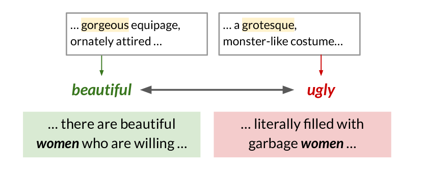
The use of “semantic axes” is enticing in that it offers an interpretable measurement of word differences beyond a single similarity value Turney and Littman (2003); An et al. (2018); Kozlowski et al. (2019); Kwak et al. (2021). Words are projected onto axes where the poles represent antonymous concepts (such as beautiful–ugly), and the projected embedding’s location along the axis indicates how similar it is to either concept. Semantic axes constructed using static, type-based embeddings have been used to analyze socially meaningful differences, such as words’ associations with class Kozlowski et al. (2019), or gender stereotypes in narratives Huang et al. (2021); Lucy and Bamman (2021b).
Our work investigates the extension and application of semantic axes to contextualized embeddings. We present a novel approach for constructing semantic axes with English BERT embeddings (Figure 1). These axes are built to encourage self-consistency, where antonymous poles are less conflated with each other. They are able to capture semantic differences across word types as well as variation in a single word across contexts. Their ability to differentiate contexts makes them suitable for studying how a word changes across domains or across individual sentences. These axes are also more self-consistent and coherent than ones created using GloVe and other baseline approaches.
We demonstrate the use of contextualized axes on two datasets: occupations from Wikipedia, and people discussed in misogynistic online communities. We use the former as a case where terms appear in definitional contexts, and characteristics of people are well-known. In the latter longitudinal, cross-platform case study, we examine lexical choices made by communities whose attitudes towards women tend to be salient and extreme. We chose this set of online communities as a substantive use case of our method, in light of recent attention in web science on analyzing online extremism and hate at scale (e.g. Ribeiro et al., 2021b, a; Aliapoulios et al., 2021). There, we analyze language change and variation along axes through a sociolinguistic lens, emphasizing that speakers use language that reflects their social identities and beliefs CH-Wang and Jurgens (2021); Huffaker and Calvert (2017); Card et al. (2016); Lakoff and Ferguson (2006).
Our code, vocabularies, and other resources can be found in our Github repo: https://github.com/lucy3/context_semantic_axes.
2 Constructing semantic axes
Static embeddings. Several formulae for calculating the similarity of a target word to two sets of pole words have been proposed in prior work on static semantic axes. These differ in whether they take the difference between a target word’s similarities to each pole Turney and Littman (2003), calculate a target word’s similarity to the difference between pole averages An et al. (2018); Kwak et al. (2021), or calculate a target word’s similarity to the average of several word pair differences that represent the same antonymous relationship Kozlowski et al. (2019). We build on the approach of An et al. (2018) and Kwak et al. (2021), because it does not require us to curate multiple paired antonyms for each axis, and it draws out the difference between two concepts before a target word is compared to them, rather than after. We define an axis containing antonymous sets of adjective vectors, and , as the following:
Relying on single-word poles for axes can be unstable to the choice of each word An et al. (2018); Antoniak and Mimno (2021). An et al. (2018) creates a pole’s set of words using the nearest neighbors of a seed word, which may risk conflating unintended meanings or antonymous neighbors Mrkšić et al. (2016); Sedoc et al. (2017). For example, one axis uses the opposite seed words green and experienced, but green’s nearest neighbors include red rather than inexperienced. Instead of using this nearest neighbors approach, we construct poles using WordNet antonym relations. Each end of an axis aggregates synonymous and similar lemmas in WordNet synsets, which are expanded using the similar to relation Miller (1992).
Our type-based embedding baseline, glove, uses 300-dimensional GloVe vectors pretrained on Wikipedia and Gigaword Pennington et al. (2014). We only keep poles where both sides have at least three adjectives that appear in the GloVe vocabulary, and we also exclude acronyms, which are often more ambiguous in meaning. We start with 723 axes, where poles have on average 9.63 adjectives each.
Contextualized embeddings. Static embeddings, however, present a number of limitations. Such embeddings cannot easily handle polysemy or homonymy Wiedemann et al. (2019), and even when they are trained on different social or temporal contexts, they require additional steps to be aligned Gonen et al. (2020). Context-specific embeddings also need enough training examples of target words to create usable representations. These limitations prevent the analysis of token-based semantic variation, such as measuring how one mention of a word is more or less beautiful than another. Our main contribution of contextualized axes uses the same WordNet-based formulation as our GloVe baseline. Rather than each word in or being represented by a single GloVe embedding, we obtain BERT embeddings over multiple occurrences of each adjective. We use BERT-base, as this model is small enough for efficient application on large datasets and is popular in previous work on semantic change and differences (e.g. Hu et al., 2019; Lucy and Bamman, 2021a; Giulianelli et al., 2020; Zhou et al., 2022; Coll Ardanuy et al., 2020; Martinc et al., 2020). It is also used in tutorials for researchers outside of NLP, which means it has high potential use in computational social science and cultural analytics Mimno et al. (2022).
For contextualized axes, we obtain a potential pool of contexts for adjectives sampled over all of Wikipedia from December 21, 2021, preprocessed using Attardi (2015)’s text extractor. This sample contains up to 1000 sentences, or contexts, that contain each adjective, and we avoid contexts that are too short (over 10 tokens) or too long (over 150 tokens).111This length cutoff made the data more manageable, and 90% of BERT’s training steps were originally on 128-length sequences Devlin et al. (2019).
We experiment with two methods of obtaining contextualized BERT embeddings for each adjective: a random “default" (bert-default) and one where contexts are picked based on word probabilities (bert-prob). For bert-default, we take a random sample of 100 contextualized embeddings across the adjectives in each pole. Since words can be nearest neighbors with their antonyms in semantic space Mrkšić et al. (2016); Sedoc et al. (2017), our main approach, bert-prob, aggregates word embeddings over contexts that highlight contrasting meanings of axes’ poles.
To select contexts, we mask out the target adjective in each of its 1000 sentences, and have BERT-base predict the probabilities of synonyms and antonyms for that masked token. We remove contexts where the average probability of antonyms is greater than that of synonyms, sort by average synonym probability, and take the top 100 contexts. One limitation of our approach is that predictions are restricted to adjectives that can be represented by one wordpiece token. If none of the words on a pole of an axis appear in BERT’s vocabulary, we backoff to bert-default to represent that axis.
For each axis type, we also have versions where words’ embeddings are -scored, which has been shown to improve BERT’s alignment with humans’ word similarity judgements Timkey and van Schijndel (2021). For -scoring, we calculate mean and standard deviation BERT embeddings from a sample of around 370k whole words from Wikipedia. As recommended by Bommasani et al. (2020), we use mean pooling over wordpieces to produce word representations when necessary, and we extend this approach to create bigram representations as well. These embeddings are a concatenation of the last four layers of BERT, as these tend to capture more context-specific information Ethayarajh (2019).
3 Internal validation
We internally validate our axes for self-consistency. For each axis, we remove one adjective’s embeddings from either side, and compute its cosine similarity to the axis constructed from the remaining adjectives. For BERT approaches, we average the adjective’s multiple embeddings to produce only one before computing its similarity to the axis. In a “consistent” axis, a left-out adjective should be closer to the pole it belongs to. That is, if it belongs to , its similarity to the axis should be positive. We average these leave-one-out similarities for each pole, negating the score when the adjective belongs to , to produce a consistency metric, . Table 1 shows for different axis-building methods.222We assign to 0 if only one unique adjective’s contexts are chosen to create a pole for bert-prob, because in that case, we are unable to run the leave-one-out test for that pole. An axis is “consistent” if both of its poles have .
glove’s most inconsistent axis poles often involve directions, such as east west, left-handed right-handed, and right left. These concepts may be difficult to learn from text without grounding. We find that the various BERT approaches’ most inconsistent axes include direction-related ones as well, but they also struggle to separate concepts such as lower-class upper-class.
The best method for producing consistent axes is -scored bert-prob, with a significant difference in from -scored bert-default and glove (Mann-Whitney U-test, ). It also produces the highest number of consistent axes. Glove presents itself as a formidable baseline,333We also tried -scoring glove embeddings, but this worsened internal consistency (). and bert-default struggles in comparison to it.
| Method | Average | # of consistent axes |
|---|---|---|
| glove | 0.101 (0.006) | 503 |
| bert-default | 0.084 (0.006) | 393 |
| bert-defaultz | 0.111 (0.007) | 468 |
| bert-prob | 0.101 (0.006) | 436 |
| bert-probz | 0.133 (0.007) | 512 |
| Category | Occupation Experiment | Person Experiment | ||
|---|---|---|---|---|
| Writing | creative, fanciful, fictive | formal, logical, discursive | + folksy, unceremonious, casual | + ignoble, common, plebeian |
| Entertainment | transcribed, taped, recorded | structural, constructive, creative | + trademarked, branded, copyrighted | + emotional, soupy, slushy |
| Art | unostentatious, aesthetic, artistic | creative, fanciful, fictive | + activist, active, hands-on | + practiced, proficient, adept |
| Health | unhealthy, pathologic, asthmatic | rehabilitative, structural, constructive | + confirmable, empirical, experiential | + teetotal, dry, drug-free |
| Agriculture | drifting, mobile, unsettled | rustic, agrarian, bucolic | + boneless, deboned, boned | - rehabilitative, structural, constructive |
| Government | amenable, answerable, responsible | policy-making, political, governmental | + respectful, deferential, honorific | + amenable, answerable, responsible |
| Sports | spry, gymnastic, sporty | zealous, ardent, enthusiastic | - amenable, answerable, responsible | - subject, subservient, dependent |
| Engineering | formal, logical, discursive | rehabilitative, structural, constructive | + coeducational, integrated, mixed | + advanced, high, graduate |
| Science | humanistic, humane, human-centered | zealous, ardent, enthusiastic | + humanistic, humane, human-centered | + stoic, unemotional, chilly |
| Math & statistics | enumerable, estimable, calculable | formal, logical, discursive | + enumerable, estimable, calculable | - amenable, answerable, responsible |
| Social Sciences | humanistic, humane, human-centered | relational, relative, comparative | + significant, portentous, probative | + humanistic, humane, human-centered |
4 External validation
Previous work on static semantic axes validates them using sentiment lexicons, exploratory analyses, and human-reported associations An et al. (2018); Kwak et al. (2021); Kozlowski et al. (2019). We perform external validation of self-consistent axes on a dataset where people appear in a variety of well-defined and known contexts: occupations from Wikipedia. We conduct two main experiments. In the first, we test whether contextualized axes can detect differences across occupation terms, and in the second, we investigate whether they can detect differences across contexts.
4.1 Data
We collect eleven categories of unigram and bigram occupations from Wikipedia lists: Writing, Entertainment, Art, Health, Agriculture, Government, Sports, Engineering, Science, Math & Statistics, and Social sciences (Appendix A). The number of occupations per category ranges from 3 in Math & Statistics to 48 in Entertainment, with an average of 27.2. We use the MediaWiki API to find Wikipedia pages for occupations in each list if they exist and follow redirects when necessary (e.g. Blogger redirects to Blog). For each occupation’s singular form, we extract sentences in its page that contains it. In total, we have 3,015 sentences for 300 occupations.
4.2 Term-level experiment (occupations)
Each occupation is represented by a pre-trained GloVe embedding or a BERT embedding averaged over all occurrences on its page. If an axis uses -scored adjective embeddings, we also -score the occupation embeddings compared to it. We assign poles to occupations based on which side of the axis they are closer to via cosine similarity. Top poles are highly related to their target occupation category, as seen by the examples for -scored bert-prob in Table 2.
One limitation for interpretability is that word embeddings’ proximity can reflect any type of semantic association, not just that a person actually has the attributes of an adjective. For example, adjectives related to unhealthy are highly associated with Health occupations, which can be explained by doctors working in environments where unhealthiness is prominent. Therefore, embedding distances only provide a foggy window into the nature of words, and this ambiguity should be considered when interpreting word similarities and their implications. This limitation applies to both static embeddings and their contextualized counterparts.
| Method | Occupation Experiment | Person Experiment |
|---|---|---|
| glove | 3.485 ( 0.491) | - |
| bert-default | 3.576 ( 0.429) | 2.697 ( 0.361) |
| bert-defaultz | 2.636 ( 0.459) | 2.485 ( 0.367) |
| bert-prob | 3.333 ( 0.473) | 2.667 ( 0.363) |
| bert-probz | 1.970 ( 0.297) | 2.152 ( 0.404) |
We conduct human evaluation on this task of using semantic axes to differentiate and characterize occupations. Three student annotators examined the top three poles retrieved by each axis-building approach and ranked these outputs based on semantic relatedness to occupation categories (Appendix B). These annotators had fair agreement, with an average Kendall’s of 0.629 across categories and experiments. Though glove is a competitive baseline, -scored bert-prob is the highest-ranked approach overall (Table 3). This suggests that more self-consistent axes also produce measurements that better reflect human judgements of occupations’ general meaning.
4.3 Context-level experiment (person)
The identity of a word, and prior associations learned from BERT’s training data, have the potential to overpower its in-context use Field and Tsvetkov (2019). Thus, we may want to discount word associations originally learned by BERT when we examine the use of a target word in a narrower context. Prior work has shown that words with higher frequency in BERT’s training data tend to encode more context-specific information in their embeddings Ethayarajh (2019); Zhou et al. (2021); Wolfe and Caliskan (2021). To investigate whether contextualized axes can measure context changes for people, we replace all occupation bigrams and unigrams with person, a very common word. This also makes contexts across different words comparable to each other, a property which we will leverage later in Section 5.4.
Each person embedding is averaged over one occupation’s contexts. The identity of person tends to overpower its similarity to axes across contexts, in that the top-ranked poles are similar across occupation categories. So, in contrast to the previous occupation experiment, additional steps are needed to draw out meaningful differences in how person is used in one group of contexts from its typical use. To do this, we estimate the average cosine similarity to axes of person embeddings in occupational contexts using 1000 bootstrapped samples, where is the number of terms in an occupation category. We take the axes with the highest statistically significant ( < 0.001, one-sample -test) difference in cosine similarity.
We assume that occupations’ Wikipedia pages mention them within definitional contexts, so top-ranked poles should reflect the original occupation replaced by person. These top poles are less intuitive than those outputted by the earlier term-level experiment (Table 2). Still, in some cases, such as for Government and Math & Statistics occupations, we uncover relative differences that distinguish one category from others. We only show three adjectives in the top two poles in Table 2 due to space considerations, but moving further down the list for -scored bert-prob uncovers additional meaningful poles. For example, the pole spry, gymnastic, sporty is the third most prominent shift and highest similarity increase (+) in the person experiment for Sports occupations. In addition, human evaluators preferred bert-prob over other approaches (Table 3, Appendix B).
5 Measuring change and variation
Now that we have contextualized semantic axes that can measure differences across words and contexts, we apply them onto a domain that can showcase salient and socially meaningful variation. NLP research on harmful language often employs methods that focus on the target group, such as measuring their association with other words Zannettou et al. (2020); Garg et al. (2018); Tahmasbi et al. (2021); Field and Tsvetkov (2019), or with biases in models Wolfe and Caliskan (2021); Ghosh et al. (2021). We illustrate the application of self-consistent -scored bert-prob axes onto the manosphere, which is a collection of communities with mostly male users who hold alternative beliefs around relationships and gender. We use the same axes we presented earlier, which were created using Wikipedia data, because Wikipedia provides more normative coverage of a variety of adjectives than topic-specific communities. This way, we examine how entities in the manosphere orient themselves against typical adjectival uses and meanings.
The manosphere has been linked to acts of violence in the physical world Hoffman et al. (2020), and most members believe that men are systemically disadvantaged in society Van Valkenburgh (2021); Marwick and Caplan (2018); Lin (2017); Ging (2019). These communities focus on heterosexual relationships and masculinity, and feature a dynamic linguistic landscape. Much prior work on the manosphere has been qualitative, such as ethnographies Lin (2017); Lumsden (2019); Van Valkenburgh (2021). There have been a few quantitative analyses of their language, usually focusing on phrase and word frequencies in a few communities Farrell et al. (2019); Gothard et al. (2021); LaViolette and Hogan (2019); Jaki et al. (2019). As an example involving word vectors, Farrell et al. (2020) uses static embeddings identify the meanings of incels’ neologisms by inspecting words’ nearest neighbors.
Our case study extends beyond prior work with its methodology and scale. We use contextualized semantic axes to tackle one question: how have references to women and contexts around them changed over fourteen years?
5.1 Data
We use a taxonomy of subreddits and external forums described by Ribeiro et al. (2021a), who show that the manosphere began with ideologies such as pick-up artists (PUA) and Men’s Rights Activists (MRA), and evolved into more extreme ones such as The Red Pill (TRP), incels (short for involuntary celibate) and Men Who Go Their Own Way (MGTOW), with users moving from older to newer ideologies. We call this dataset extreme_rel, because it contains extreme views of relationships.
We use Reddit posts and comments from March 2008 to December 2019 from subreddits listed in Ribeiro et al. (2021a)’s study, downloaded from Pushshift Baumgartner et al. (2020). We slightly modify their taxonomy by separating out incel subreddits where the intended userbase are women (femcels), and also include a newer set of subreddits focused on “Female Dating Strategy" (FDS), a women-led community analogous to TRP Holden (2020); Clark-Flory (2021). Therefore, we have 60 subreddits in seven ideological categories: Incels, MGTOW, PUA, MRA, TRP, FDS, and Femcels444The women-led communities, FDS and Femcels, make up only 1.8% of posts and comments in extreme_rel’s Reddit subset. (Appendix C). This Reddit subset of extreme_rel contains over 1.3 billion tokens.
We also include seven external forums provided by Ribeiro et al. (2021a). These public forums include A Voice for Men (AVFM), Master Pick-up Artist (MPUA) Forum, The Attraction, incels.co, MGTOW Forum, RooshV, and Red Pill Talk.555All forums are collected by Ribeiro et al. (2021a), available at https://zenodo.org/record/4007913#.YiqKexBKhQI This forum subset of extreme_rel contains over 800 million tokens spanning November 2005 to June 2019, and we remove duplicates and quoted text from posts.
Some experiments use a subset of Reddit that shares a similar topical focus as extreme_rel, but may have more mainstream views of women and relationships. We use a list666From Reddit’s List of Subreddits wiki. of common “Relationship” subreddits: r/relationships, r/dating, r/relationship_advice, r/dating_advice, and r/breakups. We call this dataset general_rel, and it contains 1.2 billion tokens from September 2009 to December 2019. For Reddit data, we do not use posts and comments written by usernames who have bot-like behavior, which we define as repeating any 10-gram more than 100 times.
5.2 Vocabulary
We use a mix of NER, online glossaries, and manual inspection to curate a unique vocabulary of people (details in Appendix D). This vocabulary has 2,434 unigrams and 4,179 bigrams, tokenized using BERT’s tokenizer without splitting words into wordpieces Devlin et al. (2019); Wolf et al. (2020). These terms appear at least 500 times in extreme_rel.
| Cluster A | Cluster B (PUA) | Cluster C (TRP, MRA) | Cluster D | Cluster E (MGTOW) | Cluster F (Incels) | ||||||
|---|---|---|---|---|---|---|---|---|---|---|---|
| she | 1.00 | girl | 1.00 | feminist | 0.93 | women | 1.00 | females | 1.00 | foids | 0.87 |
| female | 1.00 | girls | 1.00 | feminists | 0.93 | woman | 1.00 | virgin | 0.97 | foid | 0.87 |
| bitch | 0.88 | chick | 1.00 | american women | 1.00 | wife | 1.00 | whore | 0.91 | thot | 0.89 |
| girlfriend | 1.00 | chicks | 1.00 | accuser | 0.80 | mother | 1.00 | cunt | 0.77 | thots | 0.89 |
| mom | 0.97 | gf | 1.00 | accusers | 0.80 | bitches | 0.88 | most women | 1.00 | femoids | 0.89 |
Since gender is central to the manosphere, we infer these labels based on terms’ social gender in a dataset. For example, accuser is not semantically gendered like girl and woman, but its social gender, estimated using pronouns, is more feminine in extreme_rel than general_rel. We use two stages of gender inference to account for pronoun sparsity and noise. First, we use a list of semantically gendered nouns, and second, we use feminine and masculine pronouns linked to terms via coreference resolution (details in Appendix E). We label each vocabulary term based on its fraction of co-occurring feminine pronouns in extreme_rel and general_rel, separately. We are able to label 72.5% of the vocabulary in extreme_rel and 67.0% of it in general_rel.
5.3 Term-level change
Contextualized semantic axes can reveal how word and phrase types change over time. Here, our analyses focus on 1,482 feminine (gender-leaning > 0.75) terms in extreme_rel. To capture broad snapshots of words’ use, we randomly sample up to 500 sentence-level occurrences of each term in each platform and ideology (e.g. a specific forum or Reddit category) in each year. Overall -scored BERT embeddings for each vocab word are averages over this stratified sample of its contexts.
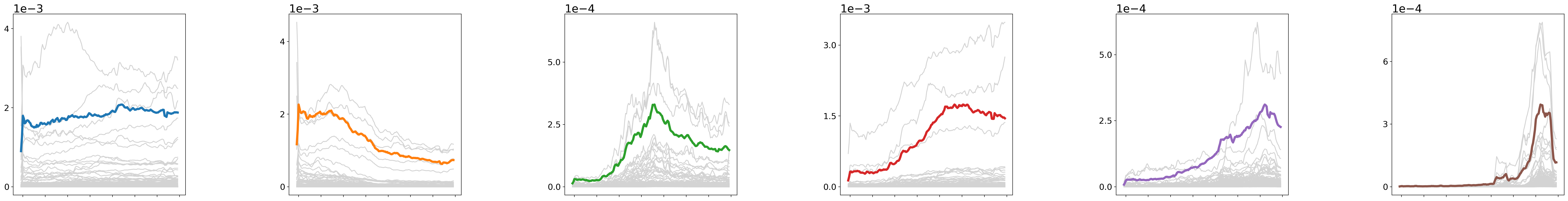
The history of the manosphere is characterized by waves of different ideological communities Ribeiro et al. (2021a). To reflect this characterization through language, we segment our vocabulary based on when terms peak in popularity. We cluster normalized frequency time series777We smooth the time series using a moving average with a kernel size of 3, and count each term once per comment to reduce the effect of unusually long comments. for each term using -Spectral Centroid clustering (KSC) Yang and Leskovec (2011). We use their default parameters, including . In contrast to their original approach, our symmetric distance measure is invariant to scaling by but not to the translation of the time series, so that peaks earlier in time are not clustered with those later in time:
where
“Waves" of term types for people correspond to ideological change. Figure 2 shows examples of feminine terms, but the top masculine terms are often labels of ideological groups, such as mgtow and incels, which we use to estimate which clusters align with ideological up and downturns.888MRA gained footing during the height of PUAs, but the peak of mras’s frequency is close to the time span’s middle. Cluster A and cluster D tend to have terms that have widespread use.
| Axis | Variance |
|---|---|
| womanly unwomanly | 0.0207 |
| androgynous male, female | 0.0105 |
| lovable detestable | 0.0104 |
| reputable disreputable | 0.0085 |
| wholesome sickening | 0.0084 |
| clean dirty | 0.0078 |
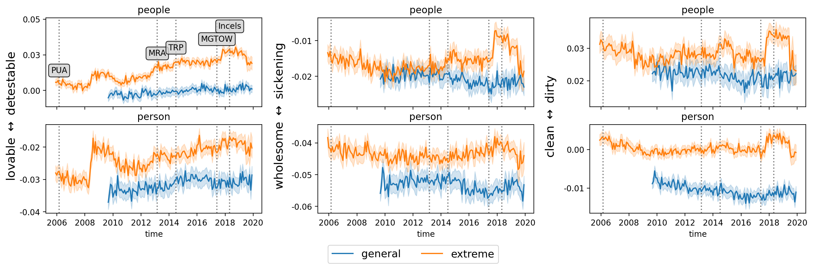
We examine the shifts of high variance, substantive axes across temporal clusters. High variance axes include those related to gender, appearance, and desirability (Table 4). For example, the lovable versus detestable pole contrasts beautiful girls with degenerate whores. As another example, the axis for clean versus dirty contrasts loyal wife with harlots. Prior studies using toxicity detection and lexicon-based approaches found that hate and misogyny rose with the arrival of later MGTOW and incel communities Farrell et al. (2019); Ribeiro et al. (2021a). Similarly, we find that lexical choices for women are more detestable and dirty in later waves associated with MGTOW and incels (Figure 3). Often, low and high frequency words share similar patterns in each wave.
5.4 Context-level change
Contextualized semantic axes can reveal how the contexts around people have changed over time. Women in online communities can be referenced in a variety of ways (Figure 2). To compare overall changes around women between mainstream and extremist communities, we examine the contexts around feminine (gender-leaning > 0.75) words. We use instances of 287 unigram types, since bigrams can include modifiers that would be considered “context”. As discussed earlier, word identities impact measurements of contextual changes across them (Section 4.3). We replace each target word with person or people depending on whether it is singular or plural, estimated through the Python inflect package. We choose replacements to respect singular/plural forms to ensure ecological validity and not perturb BERT’s sensitivity to grammaticality Yin et al. (2020). We use reservoir sampling to obtain up to 1000 occurrences of person- or people-replaced feminine words in each month on extreme_rel and general_rel.
In comparison to general_rel, extreme_rel has more detestable, sickening, and dirty contexts for women (Figure 4). Both general_rel and extreme_rel discuss relationship issues, but contextualized axes reveal how contrasting and changing attitudes toward women can influence context. Negative associations especially peak during the height of the incels’ movement around late 2017 to mid 2019. These persist despite Reddit’s ban of r/incels in November 2017 and the quarantine of r/braincels and r/theredpill in September 2018. Thus, the widespread efficacy of community-level moderation is worthy of closer study (e.g. Copland, 2020; Ribeiro et al., 2021b). An advantage of computing scores at the token-level rather than at the type-level is interpretability. That is, one can see which contexts land at the extreme ends of axes (as illustrated in Table 5).
| Example | Score |
|---|---|
| … use this against us men … those evil people! | 0.244 |
| … these people pollute our public … | 0.240 |
| … parasite worthless whore people. | 0.234 |
| … I have two little people and they are absolutely amazing … | -0.156 |
| people who are this young and attractive … | -0.144 |
| … my ideal relationship and people like this … | -0.137 |
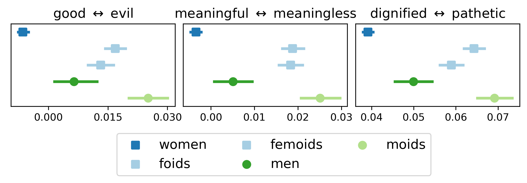
Contextualized semantic axes can also illuminate differences among lexical variables, or different linguistic forms that share the same referential meaning Nguyen et al. (2021); Labov (1972). As prominent examples, men-led communities use the lexical innovations femoids and foids, which are shortenings of female humanoids, as dehumanizing words for all women Chang (2020); Prażmo (2020). Two women-led communities, Femcels and FDS, use moids as an analogous way to refer to men. Prior work studying three manosphere subreddits showed that the lemmas woman and girl are constructed negatively as immoral, deceptive, incapable and insignificant Krendel (2020). We hypothesize that the contexts of community-specific variants should have even more dehumanizing connotations along similar dimensions. In this experiment, we replace all terms (men, moids, foids, femoids, and women) with people.
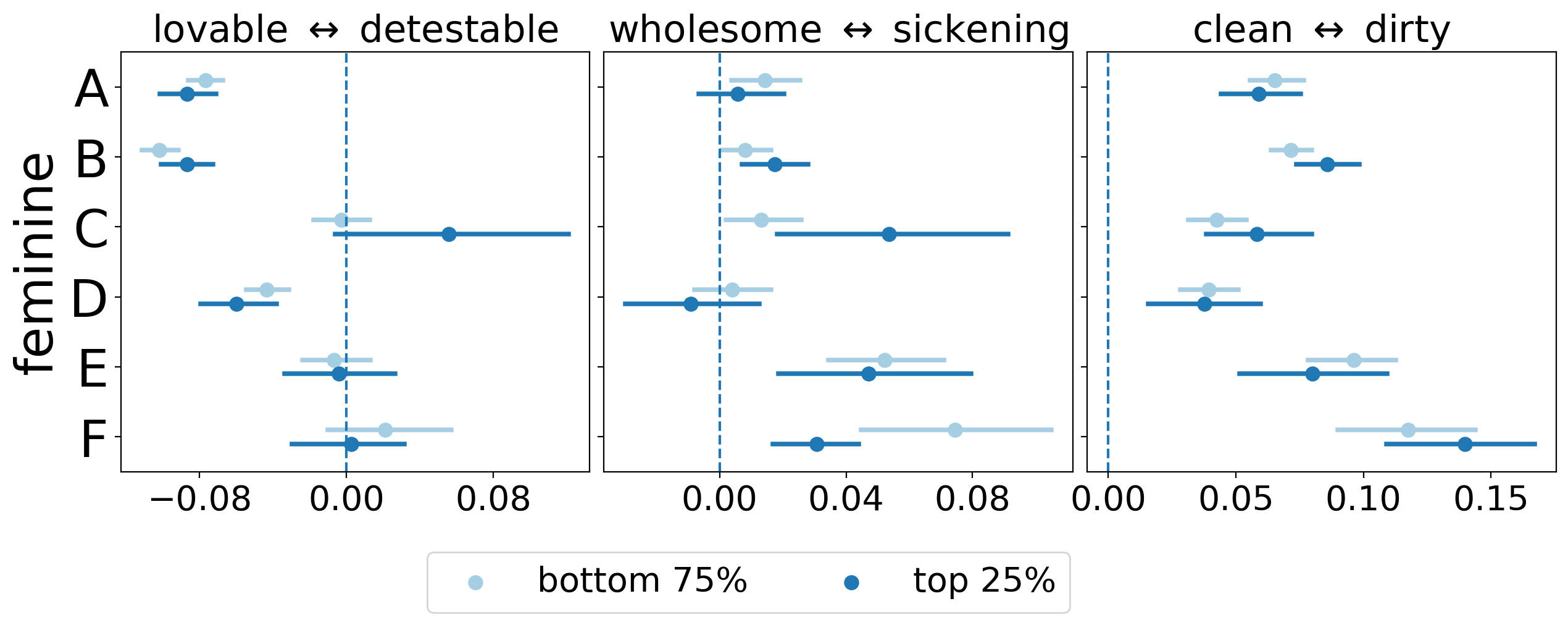
We sample up to 100 occurrences of each variant in each platform and ideology per year, limiting time ranges to when domain-specific variants are widely used by their home community. We examine the use of variants for men by Femcels and FDS in 2018-2019, and the use of variants for women by all other communities in extreme_rel in 2017-2019. Unlike in the person experiment for occupations, we have substantial pools of occurrences to compare. Thus, to find axes that distinguish one variant from another, we use axis scores as features in random forest classifiers Pedregosa et al. (2011), and perform binary classification of word identity: women versus foids or femoids, and men versus moids (Appendix G). We rank axes based on their feature importance, and select three highly ranked and relevant axes to show in Figure 5. Shifts along these axes confirm our hypothesis that community-specific variants are more dehumanized than their widely-used counterparts.
6 Conclusion
In this work, we examine the capability of contextualized embeddings for discovering differences among words and contexts. Our method uses predicted word probabilities to pinpoint which contexts to include when aggregating BERT embeddings to construct axes. This approach creates more self-consistent axes that better fit different occupation categories, in comparison to baselines. We further demonstrate the use of these axes in a longitudinal, cross-platform case study. Overall, contextualized embeddings offer more flexibility and granularity compared to static ones for the analysis of content across time and communities. That is, rather than train static word embeddings for various subsets of data, we can characterize change and variation at the token-level.
Though we focus on analyzing associations between adjectives and people, our approach can generalize to other types of entities as well. Measuring and comparing the contexts of other entity types should include many of the same considerations we did, such as reducing the conflation of antonyms, controlling for word identity by replacing target words with a shared hypernym, and experimenting with -scoring. Future work includes understanding why some opposing concepts are conflated in large language models, and how a word embedding’s identity influences its encoding of contexts.
7 Limitations
Aside from computing power requirements (Appendix H), we outline a few additional limitations of our methodology and its application not discussed in the main text.
Domain shift.
The use of pretrained BERT on a niche set of communities makes our approaches susceptible to domain shift, such as rare words having less robust embeddings Zhou et al. (2022, 2021), or target words carrying over learned associations from a broader corpus that are less applicable in a narrower one. Domain shift is difficult to avoid without retraining or further pretraining BERT, which is resource-intensive, may risk catastrophic forgetting, and inaccessible to some disciplines in computational social science Gururangan et al. (2020); Ramponi and Plank (2020); Goodfellow et al. (2014). Also, training a large language model on text with toxic and misogynistic origins introduces additional risk of dual use Kurenkov (2022). We suggest some potential workarounds that lessen the severity of domain shift, such as replacing target words with common ones for context-focused analyses.
WordNet.
WordNet is a popular lexical resource for NLP, but its senses for words can be overly fine-grained Pilehvar and Camacho-Collados (2019) and not suitable for all domains. We use WordNet version 3.0, which is included in NLTK, and this version was last updated in 2006. Since English is constantly changing, some synonym and antonym relations may be outdated.
Errors.
Our method for drawing out differences in words is better than common baselines yet still imperfect, and some of the opposing concepts in embedding space that BERT struggles to separate may be important for an application domain. Therefore, domain expertise is needed to recognize spurious patterns from real ones and fill these gaps.
In the main text we mention that embeddings offer a “foggy window” into how two concepts may be associated or related, and the exact type of relation is not always clear. For example, if contexts for women are closer to unpleasant, does it mean that the text discusses unpleasant events that affect women, or that the writers believe that women are unpleasant, or both? Some of this uncertainty could be resolved qualitatively by inspecting sentences at poles’ extremes. We compare embeddings for people to axes, but it is also possible to include relation-based approaches such as dependency parsing and compare words that share specific relations with people to axes (e.g. Lucy and Bamman, 2021b). One trade-off of doing this is that informative verbs and adjectives connected to mentions of target groups can be sparse. Our method is able to find that mathematician replaced with person is highly similar to calculable in a variety of sentence structures, such as this one modified off Wikipedia: A person is someone who uses an extensive knowledge of mathematics in their work, typically to solve mathematical problems.
8 Ethical considerations
User privacy.
Online data opens many doors for research, but its use raises concerns around user privacy. For our use case, we believe that the benefits of our work outweigh privacy-related harms. Consent is infeasible to obtain for large datasets Buchanan (2017), and in the manosphere, it is unlikely that users would give consent, especially if the researchers using their data believe that their ideologies are harmful and wrong. Obtaining consent would pose risks to the safety of the researcher Conway (2021); Doerfler et al. (2021).
All online discussions included in our work were public when downloaded by their original curators, mainly Baumgartner et al. (2020) and Ribeiro et al. (2021a). Some forums and online glossaries were relocated, shutdown, banned, or made private later on. A user’s “right to be forgotten” confronts researchers who have interests in documenting and studying the histories of communities. We truncate the examples shown in our paper rather than use them in full verbatim Bruckman (2002).
Communities may expect their posts to stay within their in-group, but the content in our work was posted on public platforms. This publicness and increased visibility plays a key role in how this content impacts others, such as those who view this information and propagate it elsewhere, or those who are direct targets of hate. Common targets such as women and people of color carry a bigger burden when participating in online spaces Hoffmann and Jonas (2017), and our broader research agenda aims to mitigate this issue.
Social biases in models and resources.
We use WordNet to group similar adjectives into semantic axes, but we observe some socially harmful associations in this resource. For example, gross and fat are listed as similar lemmas. As another example, WordNet conflates gender and sexuality when androgynous and bisexual are also listed as similar lemmas. The BERT language model, like all large, pretrained models, is also susceptible to social biases in its training data Bender et al. (2021).
Gender inference.
In this paper’s main case study, we perform gender inference for word and phrase types. This step was necessary to study how women are portrayed over time, which is a key question due to the centrality of misogyny in these communities. However, perfect prediction of each word’s perceived gender in our dataset using pronouns is impossible Cao and Daumé III (2021). Not all mentions of people co-occur with pronouns, pronouns do not equate gender, and coreference resolution systems can produce errors. So, we approximate the social gender of terms by aggregating coreference patterns over all instances of that term. Since it is difficult to separate noisy errors from meaningful word-level pronoun variation at scale, we had to use a score threshold to pinpoint what words were feminine-leaning enough to be included in our analyses.
Restricting pronouns to the traditional binary of feminine and masculine is limiting, since individuals use other pronouns as well. They/them pronouns are predominantly used to reference plural terms in this dataset, and the coreference model we use does not handle neopronouns. The manosphere and the typical framing under which it is studied is heavily cisheteronormative. We use a frequency cutoff to determine our vocabulary (Appendix D), so references to transgender and nonbinary people may be filtered out. Vocab terms retained for transgender people are outdated or typically offensive terms such as transsexuals and transgenders, and no vocab term includes non-binary, nb, or nonbinary.
9 Acknowledgements
We thank Manoel Horta Ribeiro for sharing his dataset and materials for our case study, and Sam Robertson, Alexus Lopez, and Harold Cha for evaluating model outputs. In addition, we are grateful for feedback provided by Nicholas Tomlin, Kaitlyn Zhou, and our anonymous reviewers. This research was supported by funding from the National Science Foundation (DGE-1752814, IIS-1813470, and IIS-1942591).
References
- Aliapoulios et al. (2021) Max Aliapoulios, Kejsi Take, Prashanth Ramakrishna, Daniel Borkan, Beth Goldberg, Jeffrey Sorensen, Anna Turner, Rachel Greenstadt, Tobias Lauinger, and Damon McCoy. 2021. A large-scale characterization of online incitements to harassment across platforms. In Proceedings of the 21st ACM Internet Measurement Conference, IMC ’21, page 621–638, New York, NY, USA. Association for Computing Machinery.
- An et al. (2018) Jisun An, Haewoon Kwak, and Yong-Yeol Ahn. 2018. SemAxis: A lightweight framework to characterize domain-specific word semantics beyond sentiment. In Proceedings of the 56th Annual Meeting of the Association for Computational Linguistics (Volume 1: Long Papers), pages 2450–2461, Melbourne, Australia. Association for Computational Linguistics.
- Antoniak and Mimno (2021) Maria Antoniak and David Mimno. 2021. Bad seeds: Evaluating lexical methods for bias measurement. In Proceedings of the 59th Annual Meeting of the Association for Computational Linguistics and the 11th International Joint Conference on Natural Language Processing (Volume 1: Long Papers), pages 1889–1904, Online. Association for Computational Linguistics.
- Attardi (2015) Giusepppe Attardi. 2015. Wikiextractor. https://github.com/attardi/wikiextractor.
- Baumgartner et al. (2020) Jason Baumgartner, Savvas Zannettou, Brian Keegan, Megan Squire, and Jeremy Blackburn. 2020. The pushshift reddit dataset. In Proceedings of the international AAAI conference on web and social media, volume 14, pages 830–839.
-
Bender et al. (2021)
Emily M. Bender, Timnit Gebru, Angelina McMillan-Major, and Shmargaret
Shmitchell. 2021.
On the dangers of
stochastic parrots: Can language models be too
big?
![[Uncaptioned image]](/html/2210.12170/assets/parrot.png) .
In Proceedings of the 2021 ACM Conference on Fairness,
Accountability, and Transparency, FAccT ’21, page 610–623, New York, NY,
USA. Association for Computing Machinery.
.
In Proceedings of the 2021 ACM Conference on Fairness,
Accountability, and Transparency, FAccT ’21, page 610–623, New York, NY,
USA. Association for Computing Machinery.
- Beran (2018) Dale Beran. 2018. Who are the incels of 4chan and why are they so angry? https://psmag.com/news/who-are-the-incels-of-4chan-and-why-are-they-so-angry.
- Bommasani et al. (2020) Rishi Bommasani, Kelly Davis, and Claire Cardie. 2020. Interpreting Pretrained Contextualized Representations via Reductions to Static Embeddings. In Proceedings of the 58th Annual Meeting of the Association for Computational Linguistics, pages 4758–4781, Online. Association for Computational Linguistics.
- Bruckman (2002) Amy Bruckman. 2002. Studying the amateur artist: A perspective on disguising data collected inhuman subjects research on the internet. Ethics and Inf. Technol., 4(3):217–231.
- Buchanan (2017) Elizabeth Buchanan. 2017. Considering the ethics of big data research: A case of Twitter and ISIS/ISIL. PLOS ONE, 12(12):1–6.
- Cao and Daumé III (2021) Yang Trista Cao and Hal Daumé III. 2021. Toward gender-inclusive coreference resolution: An analysis of gender and bias throughout the machine learning lifecycle*. Computational Linguistics, 47(3):615–661.
- Card et al. (2016) Dallas Card, Justin Gross, Amber Boydstun, and Noah A. Smith. 2016. Analyzing framing through the casts of characters in the news. In Proceedings of the 2016 Conference on Empirical Methods in Natural Language Processing, pages 1410–1420, Austin, Texas. Association for Computational Linguistics.
- CH-Wang and Jurgens (2021) Sky CH-Wang and David Jurgens. 2021. Using sociolinguistic variables to reveal changing attitudes towards sexuality and gender. In Proceedings of the 2021 Conference on Empirical Methods in Natural Language Processing, pages 9918–9938, Online and Punta Cana, Dominican Republic. Association for Computational Linguistics.
- Chang (2020) Winnie Chang. 2020. The monstrous-feminine in the incel imagination: investigating the representation of women as “femoids” on /r/braincels. Feminist Media Studies, 0(0):1–17.
- Charlesworth et al. (2022) Tessa E. S. Charlesworth, Aylin Caliskan, and Mahzarin R. Banaji. 2022. Historical representations of social groups across 200 years of word embeddings from google books. Proceedings of the National Academy of Sciences, 119(28):e2121798119.
- Clark and Manning (2016) Kevin Clark and Christopher D. Manning. 2016. Deep reinforcement learning for mention-ranking coreference models. In Proceedings of the 2016 Conference on Empirical Methods in Natural Language Processing, pages 2256–2262, Austin, Texas. Association for Computational Linguistics.
- Clark-Flory (2021) Tracy Clark-Flory. 2021. Reddit’s Female Dating Strategy, advice for ‘queens’. https://jezebel.com/inside-female-dating-strategy-the-subreddit-that-teach-1847558145.
- Coll Ardanuy et al. (2020) Mariona Coll Ardanuy, Federico Nanni, Kaspar Beelen, Kasra Hosseini, Ruth Ahnert, Jon Lawrence, Katherine McDonough, Giorgia Tolfo, Daniel CS Wilson, and Barbara McGillivray. 2020. Living machines: A study of atypical animacy. In Proceedings of the 28th International Conference on Computational Linguistics, pages 4534–4545, Barcelona, Spain (Online). International Committee on Computational Linguistics.
- Conway (2021) Maura Conway. 2021. Online extremism and terrorism research ethics: Researcher safety, informed consent, and the need for tailored guidelines. Terrorism and Political Violence, 33(2):367–380.
- Copland (2020) Simon Copland. 2020. Reddit quarantined: Can changing platform affordances reduce hateful material online? Internet Policy Review: Journal on Internet Regulation, 9(4):1–26.
- Devlin et al. (2019) Jacob Devlin, Ming-Wei Chang, Kenton Lee, and Kristina Toutanova. 2019. BERT: Pre-training of deep bidirectional transformers for language understanding. In Proceedings of the 2019 Conference of the North American Chapter of the Association for Computational Linguistics: Human Language Technologies, Volume 1 (Long and Short Papers), pages 4171–4186, Minneapolis, Minnesota. Association for Computational Linguistics.
- Doerfler et al. (2021) Periwinkle Doerfler, Andrea Forte, Emiliano De Cristofaro, Gianluca Stringhini, Jeremy Blackburn, and Damon McCoy. 2021. "I’m a professor, which isn’t usually a dangerous job": Internet-facilitated harassment and its impact on researchers. Proc. ACM Hum.-Comput. Interact., 5(CSCW2).
- Ethayarajh (2019) Kawin Ethayarajh. 2019. How contextual are contextualized word representations? Comparing the geometry of BERT, ELMo, and GPT-2 embeddings. In Proceedings of the 2019 Conference on Empirical Methods in Natural Language Processing and the 9th International Joint Conference on Natural Language Processing (EMNLP-IJCNLP), pages 55–65, Hong Kong, China. Association for Computational Linguistics.
- Farrell et al. (2020) Tracie Farrell, Oscar Araque, Miriam Fernandez, and Harith Alani. 2020. On the use of jargon and word embeddings to explore subculture within the Reddit’s manosphere. In 12th ACM Conference on Web Science, WebSci ’20, page 221–230, New York, NY, USA. Association for Computing Machinery.
- Farrell et al. (2019) Tracie Farrell, Miriam Fernandez, Jakub Novotny, and Harith Alani. 2019. Exploring misogyny across the manosphere in reddit. In Proceedings of the 10th ACM Conference on Web Science, pages 87–96.
- Field and Tsvetkov (2019) Anjalie Field and Yulia Tsvetkov. 2019. Entity-centric contextual affective analysis. In Proceedings of the 57th Annual Meeting of the Association for Computational Linguistics, pages 2550–2560, Florence, Italy. Association for Computational Linguistics.
- Fraser et al. (2021) Kathleen C. Fraser, Isar Nejadgholi, and Svetlana Kiritchenko. 2021. Understanding and countering stereotypes: A computational approach to the stereotype content model. In Proceedings of the 59th Annual Meeting of the Association for Computational Linguistics and the 11th International Joint Conference on Natural Language Processing (Volume 1: Long Papers), pages 600–616, Online. Association for Computational Linguistics.
- Garg et al. (2018) Nikhil Garg, Londa Schiebinger, Dan Jurafsky, and James Zou. 2018. Word embeddings quantify 100 years of gender and ethnic stereotypes. Proceedings of the National Academy of Sciences, 115(16):E3635–E3644.
- Ghosh et al. (2021) Sayan Ghosh, Dylan Baker, David Jurgens, and Vinodkumar Prabhakaran. 2021. Detecting cross-geographic biases in toxicity modeling on social media. In Proceedings of the Seventh Workshop on Noisy User-generated Text (W-NUT 2021), pages 313–328, Online. Association for Computational Linguistics.
- Ging (2019) Debbie Ging. 2019. Alphas, betas, and incels: Theorizing the masculinities of the manosphere. Men and Masculinities, 22(4):638–657.
- Giulianelli et al. (2020) Mario Giulianelli, Marco Del Tredici, and Raquel Fernández. 2020. Analysing lexical semantic change with contextualised word representations. In Proceedings of the 58th Annual Meeting of the Association for Computational Linguistics, pages 3960–3973, Online. Association for Computational Linguistics.
- Gonen et al. (2020) Hila Gonen, Ganesh Jawahar, Djamé Seddah, and Yoav Goldberg. 2020. Simple, interpretable and stable method for detecting words with usage change across corpora. In Proceedings of the 58th Annual Meeting of the Association for Computational Linguistics, pages 538–555, Online. Association for Computational Linguistics.
- Goodfellow et al. (2014) Ian J. Goodfellow, Mehdi Mirza, Da Xiao, Aaron Courville, and Yoshua Bengio. 2014. An empirical investigation of catastrophic forgeting in gradientbased neural networks. In In Proceedings of International Conference on Learning Representations (ICLR).
- Gothard et al. (2021) Kelly Gothard, David Rushing Dewhurst, Joshua A. Minot, Jane Lydia Adams, Christopher M. 5-Danforth, and Peter Sheridan Dodds. 2021. The incel lexicon: Deciphering the emergent cryptolect of a global misogynistic community. Available online at https://arxiv.org/abs/2105.12006.
- Grand et al. (2022) Gabriel Grand, Idan Asher Blank, Francisco Pereira, and Evelina Fedorenko. 2022. Semantic projection recovers rich human knowledge of multiple object features from word embeddings. Nature Human Behaviour, pages 1–13.
- Gururangan et al. (2020) Suchin Gururangan, Ana Marasović, Swabha Swayamdipta, Kyle Lo, Iz Beltagy, Doug Downey, and Noah A. Smith. 2020. Don’t stop pretraining: Adapt language models to domains and tasks. In Proceedings of the 58th Annual Meeting of the Association for Computational Linguistics, pages 8342–8360, Online. Association for Computational Linguistics.
- Hamilton et al. (2016) William L. Hamilton, Jure Leskovec, and Dan Jurafsky. 2016. Cultural shift or linguistic drift? comparing two computational measures of semantic change. In Proceedings of the 2016 Conference on Empirical Methods in Natural Language Processing, pages 2116–2121, Austin, Texas. Association for Computational Linguistics.
- Hoffman et al. (2020) Bruce Hoffman, Jacob Ware, and Ezra Shapiro. 2020. Assessing the threat of incel violence. Studies in Conflict & Terrorism, 43(7):565–587.
- Hoffmann and Jonas (2017) Anna Lauren Hoffmann and Anne Jonas. 2017. Recasting Justice for Internet and Online Industry Research Ethics, Internet Research Ethics for the Social Age: New Cases and Challenges, pages 3–18. Peter Lang.
- Holden (2020) Madeleine Holden. 2020. Reddit Female Dating Strategy: ‘like Red Pill for women’. https://melmagazine.com/en-us/story/female-dating-strategy-reddit.
- Hoyle et al. (2019) Alexander Miserlis Hoyle, Lawrence Wolf-Sonkin, Hanna Wallach, Isabelle Augenstein, and Ryan Cotterell. 2019. Unsupervised discovery of gendered language through latent-variable modeling. In Proceedings of the 57th Annual Meeting of the Association for Computational Linguistics, pages 1706–1716, Florence, Italy. Association for Computational Linguistics.
- Hu et al. (2019) Renfen Hu, Shen Li, and Shichen Liang. 2019. Diachronic sense modeling with deep contextualized word embeddings: An ecological view. In Proceedings of the 57th Annual Meeting of the Association for Computational Linguistics, pages 3899–3908, Florence, Italy. Association for Computational Linguistics.
- Huang et al. (2021) Tenghao Huang, Faeze Brahman, Vered Shwartz, and Snigdha Chaturvedi. 2021. Uncovering implicit gender bias in narratives through commonsense inference. In Findings of the Association for Computational Linguistics: EMNLP 2021, pages 3866–3873, Punta Cana, Dominican Republic. Association for Computational Linguistics.
- Huffaker and Calvert (2017) David A. Huffaker and Sandra L. Calvert. 2017. Gender, Identity, and Language Use in Teenage Blogs. Journal of Computer-Mediated Communication, 10(2). JCMC10211.
- Jaki et al. (2019) Sylvia Jaki, Tom De Smedt, Maja Gwóźdź, Rudresh Panchal, Alexander Rossa, and Guy De Pauw. 2019. Online hatred of women in the incels.me forum: Linguistic analysis and automatic detection. Journal of Language Aggression and Conflict, 7(2):240–268.
- Kozlowski et al. (2019) Austin C Kozlowski, Matt Taddy, and James A Evans. 2019. The geometry of culture: Analyzing the meanings of class through word embeddings. American Sociological Review, 84(5):905–949.
- Krendel (2020) Alexandra Krendel. 2020. The men and women, guys and girls of the ‘manosphere’: A corpus-assisted discourse approach. Discourse & Society, 31(6):607–630.
- Kurenkov (2022) Andrey Kurenkov. 2022. Lessons from the GPT-4chan controversy. The Gradient.
- Kwak et al. (2021) Haewoon Kwak, Jisun An, Elise Jing, and Yong-Yeol Ahn. 2021. Frameaxis: characterizing microframe bias and intensity with word embedding. PeerJ Computer Science, 7:e644.
- Labov (1972) William Labov. 1972. Sociolinguistic patterns. 4. University of Pennsylvania press.
- Lakoff and Ferguson (2006) George Lakoff and Sam Ferguson. 2006. The framing of immigration. Rockridge Institute.
- LaViolette and Hogan (2019) Jack LaViolette and Bernie Hogan. 2019. Using platform signals for distinguishing discourses: The case of men’s rights and men’s liberation on reddit. Proceedings of the International AAAI Conference on Web and Social Media, 13(01):323–334.
- Lin (2017) Jie Liang Lin. 2017. Antifeminism Online: MGTOW (Men Going Their Own Way), pages 77–96. transcript Verlag.
- Lucy and Bamman (2021a) Li Lucy and David Bamman. 2021a. Characterizing English variation across social media communities with BERT. Transactions of the Association for Computational Linguistics, 9:538–556.
- Lucy and Bamman (2021b) Li Lucy and David Bamman. 2021b. Gender and representation bias in GPT-3 generated stories. In Proceedings of the Third Workshop on Narrative Understanding, pages 48–55, Virtual. Association for Computational Linguistics.
- Lumsden (2019) Karen Lumsden. 2019. “‘I Want to Kill You in Front of Your Children” Is Not a Threat. It’s an Expression of a Desire’: Discourses of Online Abuse, Trolling and Violence on r/MensRights, pages 91–115. Springer International Publishing, Cham.
- Martinc et al. (2020) Matej Martinc, Petra Kralj Novak, and Senja Pollak. 2020. Leveraging contextual embeddings for detecting diachronic semantic shift. In Proceedings of the 12th Language Resources and Evaluation Conference, pages 4811–4819, Marseille, France. European Language Resources Association.
- Marwick and Caplan (2018) Alice E. Marwick and Robyn Caplan. 2018. Drinking male tears: language, the manosphere, and networked harassment. Feminist Media Studies, 18(4):543–559.
- Mathew et al. (2020) Binny Mathew, Sandipan Sikdar, Florian Lemmerich, and Markus Strohmaier. 2020. The POLAR framework: Polar opposites enable interpretability of pre-trained word embeddings. In Proceedings of The Web Conference 2020, WWW ’20, page 1548–1558, New York, NY, USA. Association for Computing Machinery.
- Mendelsohn et al. (2020) Julia Mendelsohn, Yulia Tsvetkov, and Dan Jurafsky. 2020. A framework for the computational linguistic analysis of dehumanization. Frontiers in Artificial Intelligence, 3.
- Miller (1992) George A. Miller. 1992. WordNet: A lexical database for English. In Speech and Natural Language: Proceedings of a Workshop Held at Harriman, New York, February 23-26, 1992.
- Mimno et al. (2022) David Mimno, Melanie Walsh, and Maria Antoniak. 2022. BERT for humanists. http://www.bertforhumanists.org/.
- Mrkšić et al. (2016) Nikola Mrkšić, Diarmuid Ó Séaghdha, Blaise Thomson, Milica Gašić, Lina M. Rojas-Barahona, Pei-Hao Su, David Vandyke, Tsung-Hsien Wen, and Steve Young. 2016. Counter-fitting word vectors to linguistic constraints. In Proceedings of the 2016 Conference of the North American Chapter of the Association for Computational Linguistics: Human Language Technologies, pages 142–148, San Diego, California. Association for Computational Linguistics.
- Nguyen et al. (2021) Dong Nguyen, Laura Rosseel, and Jack Grieve. 2021. On learning and representing social meaning in NLP: a sociolinguistic perspective. In Proceedings of the 2021 Conference of the North American Chapter of the Association for Computational Linguistics: Human Language Technologies, pages 603–612, Online. Association for Computational Linguistics.
- Pedregosa et al. (2011) F. Pedregosa, G. Varoquaux, A. Gramfort, V. Michel, B. Thirion, O. Grisel, M. Blondel, P. Prettenhofer, R. Weiss, V. Dubourg, J. Vanderplas, A. Passos, D. Cournapeau, M. Brucher, M. Perrot, and E. Duchesnay. 2011. Scikit-learn: Machine learning in Python. Journal of Machine Learning Research, 12:2825–2830.
- Pennington et al. (2014) Jeffrey Pennington, Richard Socher, and Christopher Manning. 2014. GloVe: Global vectors for word representation. In Proceedings of the 2014 Conference on Empirical Methods in Natural Language Processing (EMNLP), pages 1532–1543, Doha, Qatar. Association for Computational Linguistics.
- Pilehvar and Camacho-Collados (2019) Mohammad Taher Pilehvar and Jose Camacho-Collados. 2019. WiC: the word-in-context dataset for evaluating context-sensitive meaning representations. In Proceedings of the 2019 Conference of the North American Chapter of the Association for Computational Linguistics: Human Language Technologies, Volume 1 (Long and Short Papers), pages 1267–1273, Minneapolis, Minnesota. Association for Computational Linguistics.
- Prażmo (2020) Ewelina Prażmo. 2020. Foids are worse than animals. A cognitive linguistics analysis of dehumanizing metaphors in online discourse. Topics in Linguistics, 21:16–27.
- Ramponi and Plank (2020) Alan Ramponi and Barbara Plank. 2020. Neural unsupervised domain adaptation in NLP—A survey. In Proceedings of the 28th International Conference on Computational Linguistics, pages 6838–6855, Barcelona, Spain (Online). International Committee on Computational Linguistics.
- Ribeiro et al. (2021a) Manoel Horta Ribeiro, Jeremy Blackburn, Barry Bradlyn, Emiliano De Cristofaro, Gianluca Stringhini, Summer Long, Stephanie Greenberg, and Savvas Zannettou. 2021a. The evolution of the manosphere across the web. In Proceedings of the International AAAI Conference on Web and Social Media, volume 15, pages 196–207.
- Ribeiro et al. (2021b) Manoel Horta Ribeiro, Shagun Jhaver, Savvas Zannettou, Jeremy Blackburn, Gianluca Stringhini, Emiliano De Cristofaro, and Robert West. 2021b. Do platform migrations compromise content moderation? evidence from r/The_Donald and r/Incels. Proc. ACM Hum.-Comput. Interact., 5(CSCW2).
- Sedoc et al. (2017) João Sedoc, Jean Gallier, Dean Foster, and Lyle Ungar. 2017. Semantic word clusters using signed spectral clustering. In Proceedings of the 55th Annual Meeting of the Association for Computational Linguistics (Volume 1: Long Papers), pages 939–949, Vancouver, Canada. Association for Computational Linguistics.
- Sonnad and Squirrell (2019) Nikhil Sonnad and Tim Squirrell. 2019. The alt-right is creating its own dialect. Here’s the dictionary. https://qz.com/1092037/the-alt-right-is-creating-its-own-dialect-heres-a-complete-guide/.
- Squirrell (2018) Tim Squirrell. 2018. A definitive guide to Incels part two: the a-z incel dictionary. https://www.timsquirrell.com/blog/2018/5/30/a-definitive-guide-to-incels-part-two-the-blackpill-and-vocabulary.
- Tahmasbi et al. (2021) Fatemeh Tahmasbi, Leonard Schild, Chen Ling, Jeremy Blackburn, Gianluca Stringhini, Yang Zhang, and Savvas Zannettou. 2021. “Go Eat a Bat, Chang!”: On the emergence of sinophobic behavior on web communities in the face of COVID-19. In Proceedings of the Web Conference 2021, WWW ’21, page 1122–1133, New York, NY, USA. Association for Computing Machinery.
- Timkey and van Schijndel (2021) William Timkey and Marten van Schijndel. 2021. All bark and no bite: Rogue dimensions in transformer language models obscure representational quality. In Proceedings of the 2021 Conference on Empirical Methods in Natural Language Processing, pages 4527–4546, Online and Punta Cana, Dominican Republic. Association for Computational Linguistics.
- Turney and Littman (2003) Peter D Turney and Michael L Littman. 2003. Measuring praise and criticism: Inference of semantic orientation from association. ACM Transactions on Information Systems (TOIS), 21(4):315–346.
- Van Valkenburgh (2021) Shawn P Van Valkenburgh. 2021. Digesting the red pill: Masculinity and neoliberalism in the manosphere. Men and Masculinities, 24(1):84–103.
- Wiedemann et al. (2019) Gregor Wiedemann, Steffen Remus, Avi Chawla, and Chris Biemann. 2019. Does BERT make any sense? interpretable word sense disambiguation with contextualized embeddings. In Proceedings of the 15th Conference on Natural Language Processing (KONVENS 2019): Long Papers, pages 161–170, Erlangen, Germany. German Society for Computational Linguistics & Language Technology.
- Wolf et al. (2020) Thomas Wolf, Lysandre Debut, Victor Sanh, Julien Chaumond, Clement Delangue, Anthony Moi, Pierric Cistac, Tim Rault, Remi Louf, Morgan Funtowicz, Joe Davison, Sam Shleifer, Patrick von Platen, Clara Ma, Yacine Jernite, Julien Plu, Canwen Xu, Teven Le Scao, Sylvain Gugger, Mariama Drame, Quentin Lhoest, and Alexander Rush. 2020. Transformers: State-of-the-art natural language processing. In Proceedings of the 2020 Conference on Empirical Methods in Natural Language Processing: System Demonstrations, pages 38–45, Online. Association for Computational Linguistics.
- Wolfe and Caliskan (2021) Robert Wolfe and Aylin Caliskan. 2021. Low frequency names exhibit bias and overfitting in contextualizing language models. In Proceedings of the 2021 Conference on Empirical Methods in Natural Language Processing, pages 518–532, Online and Punta Cana, Dominican Republic. Association for Computational Linguistics.
- Yang and Leskovec (2011) Jaewon Yang and Jure Leskovec. 2011. Patterns of temporal variation in online media. In Proceedings of the Fourth ACM International Conference on Web Search and Data Mining, WSDM ’11, page 177–186, New York, NY, USA. Association for Computing Machinery.
- Yin et al. (2020) Fan Yin, Quanyu Long, Tao Meng, and Kai-Wei Chang. 2020. On the robustness of language encoders against grammatical errors. In Proceedings of the 58th Annual Meeting of the Association for Computational Linguistics, pages 3386–3403, Online. Association for Computational Linguistics.
- Zannettou et al. (2020) Savvas Zannettou, Joel Finkelstein, Barry Bradlyn, and Jeremy Blackburn. 2020. A quantitative approach to understanding online antisemitism. In Proceedings of the International AAAI Conference on Web and Social Media, volume 14, pages 786–797.
- Zhou et al. (2021) Kaitlyn Zhou, Kawin Ethayarajh, and Dan Jurafsky. 2021. Frequency-based distortions in contextualized word embeddings. arXiv preprint arXiv:2104.08465.
- Zhou et al. (2022) Kaitlyn Zhou, Kawin Ethayarajh, and Dan Jurafsky. 2022. Richer countries and richer representations. In Findings of the Association for Computational Linguistics: ACL 2022, pages 2074–2085, Dublin, Ireland. Association for Computational Linguistics.
Appendix A Wikipedia page titles
Table 6 lists the categories of occupations, the titles of Wikipedia pages that list them, and the number of terms in each category. These lists were retrieved in February 2022.
Appendix B Human evaluation for occupations
We recruited three student volunteers with familiarity with NLP coursework and tasks to rank the top poles provided by each axis-building method for our occupation and person experiments. We used Qualtrics to design and launch the survey. Since we were not asking about personal opinions but rather evaluating models, we were determined exempt from IRB review by the appropriate office at our institution. Each question pertains to a specific occupation category, and within each experiment, question order and answer option order are randomly shuffled. Each model option is presented with its top three poles, in order of most to less relevant. Figure 6 shows screenshots of instructions. In the toy example, the options are labeled with “Model A", “Model B", “Model C", to allow explanation clarity, but in the actual task questions, options are not labeled with model letters to avoid biasing the evaluators towards a specific model. Some annotators expressed that the task was difficult, and for some occupations, different approaches output similar axes, just in different order.
| Occupation type | Wikipedia category lists | # of terms |
|---|---|---|
| Writing | “List of writing occupations" | 27 |
| Entertainment | “List of theatre personnel", “List of film and television occupations" | 48 |
| Art | “List of artistic occupations" | 32 |
| Health | “List of healthcare occupations" | 47 |
| Agriculture | “Category:Agricultural occupations", and plant and husbandry subcategory | 29 |
| Government | “Category:Government occupations" | 47 |
| Sports | “Lists of sportspeople" | 24 |
| Engineering | “List of scientific occupations" | 7 |
| Physical, natural, and earth sciences (“Science”) | “List of scientific occupations" | 30 |
| Math & statistics | “List of scientific occupations" | 3 |
| Social sciences | “List of scientific occupations" | 6 |
Appendix C Reddit communities
We used a list of subreddits999This list can be found at our Github repo: https://github.com/lucy3/context_semantic_axes. for the manosphere provided by Ribeiro et al. (2021a) in their detailed, data-driven sketch of the manosphere.
Five of the subreddits included in Ribeiro et al. (2021a)’s taxonomy of the Reddit manosphere (r/malecels, r/lonelynonviolentmen, r/1ncels, r/incelbrotherhood, r/incelspurgatory) were not on Pushshift’s dump of Reddit. We curated the list of communities for our new ideological category, Female Dating Strategy (FDS), using a now removed list of FDS’s “sister communities" on the subreddit r/FemaleDatingStrategy’s sidebar: r/PinkpillFeminism, r/AskFDS, r/FDSSuperFans, r/PornFreeRelationships, and r/FemaleLevelUpStrategy. The Femcels set of subreddits include: r/Trufemcels, r/TheGlowUp, and r/AskTruFemcels. Though the main user base of the manosphere are men, there are also small populations of women in other ideologies as well, such as r/redpillwomen. We mainly portion out FDS and Femcels due to their role in Section 5.4’s lexical variant experiment as communities who use moids.
In total we have 12 subreddits in TRP, 11 in MRA, 7 in PUA, 22 in Incels, 3 in MGTOW, 4 in Femcels, and 6 in FDS. The complete list of subreddits and their categories is also in our Github repo.
Appendix D Vocabulary creation
First, we extract nominal and proper persons using NER, keeping ones that are popular (occur at least 500 times in extreme_rel), and unambiguous, where at least 20% of its instances in these datasets are tagged as a person. Gathering a substantial number of labels from our domain to train an in-domain NER system from scratch is outside the scope of our work, so we experimented with three models trained on other labeled datasets: ACE, contemporary literature, and a combination of both. We evaluated these models on a small set of posts and comments labeled by one author, after retrieving 25 examples per forum or Reddit ideological category using reservoir sampling. The annotator only labeled spans for nominal and named Person entities. Table 7 shows the performance of each model on extreme_rel. Based on these evaluation results, we chose to use the model trained on contemporary literature.
We extract bigrams and unigrams from detected spans, excluding determiners and possessives whose heads are the root of the span. Named entities that refer to types of people rather than specific individuals were estimated through their co-occurrence with the determiner a, e.g. a Chad.
| Training data | Precision | Recall | F1 |
|---|---|---|---|
| ACE | 0.657 | 0.641 | 0.649 |
| Literature | 0.798 | 0.711 | 0.752 |
| Combined | 0.715 | 0.744 | 0.729 |
Then, one author consulted community glossaries and examined in-context use of words to manually correct the list of automatically extracted terms. We include additional popular and unambiguous words not tagged sufficiently often enough by NER, but defined as people in prior work and online resources.
Table 8 lists the sources and glossaries for vocabulary words and the ideologies they include. Some of these sources, such as the Shedding of the Ego, are created by insiders in the community, while some, such as academic papers and news articles, are by outsiders. For each of these glossaries and lists of terms, we manually separated them into two categories: 269 people (singular and plural forms) and 1776 non-people. Two of these sites, Shedding of the Ego and Pualingo, no longer exists, but were publicly available until at least late 2020. We include 93 terms for people that were initially filtered out in our NER pipeline in our final vocabulary, excluding ambiguous ones that also occur often as non-human entities, such as tool (a fool who is taken advantage of) and jaw (short for just another wannabe).
The resulting vocabulary contains niche language, where 20.7% of unigrams are not found in WordNet, and 85.1% of those missing are also not in the Internet resource Urban Dictionary.101010We use the naive approach of adding or removing ‘-s’ to search for either plural or singular forms in these lexicons. The full list is also available in our Github repo.
| Source | Medium | Community |
|---|---|---|
| Jaki et al. (2019) | academic paper | Incels |
| Ging (2019) | academic paper | Manosphere |
| Farrell et al. (2019) | academic paper | Manosphere |
| Lin (2017) | academic paper | MGTOW |
| Squirrell (2018) | blog | Incels |
| Sonnad and Squirrell (2019) | news | Red Pill |
| Beran (2018) | magazine | Incels |
| Pualingo | website | PUA |
| Rational Wiki | website | Manosphere |
| Shedding of the Ego | blog | MGTOW, PUA |
Appendix E Gender inference
This section includes additional details around our gender inference process.
Our list of semantically gendered terms, or words gendered by definition, expands upon the one used by Hoyle et al. (2019): man, men, boy, boys, father, fathers, son, sons, brother, bothers, husband, husbands, uncle, uncles, nephew, nephews, emperor, emperors, king, kings, prince, princes, duke, dukes, lord, lords, knight, knights, waiter, waiters, actor, actors, god, gods, policeman, policemen, postman, postmen, hero, heros, wizard, wizards, steward, stewards, woman, women, girl, girls, mother, mothers, daughter, daughters, sister, sisters, wife, wives, aunt, aunts, niece, nieces, empress, empresses, queen, queens, princess, princesses, duchess, duchesses, lady, ladies, dame, dames, waitress, waitresses, actress, actresses, goddess, goddesses, policewoman, policewomen, postwoman, postwomen, heroine, heroines, witch, witches, stewardess, stewardesses.
We include the following additional semantically gendered terms: male, males, dude, dudes, guy, guys, boyfriend, boyfriends, bf, female, females, chick, chicks, girlfriend, girlfriends, gf, gal, gals, bro, transmen, transwomen, she, he.
We check if any of the above words appear in a unigram or bigram vocabularly term. Around 29.9% of our vocabulary in extreme_rel is gendered through this word list approach.
| Feminine | ||
|---|---|---|
| Axis | Variance | Examples |
| womanly unwomanly | 0.0207 | female gender, feminine women, feminine woman hambeast, tomboys, tomboy |
| androgynous male, female | 0.0105 | manipulative bitch, nympho, noodlewhore white females, female, females |
| lovable detestable | 0.0101 | little princess, sweet girl, beautiful girl stupid cunts, degenerate whores, accusers |
| reputable disreputable | 0.0085 | great wife, great woman, great women slut, dirty slut, sluts |
| wholesome sickening | 0.0084 | homemakers, healthy woman, healthy women evil bitch, dirty slut, degenerate whores |
| clean dirty | 0.0078 | loyal wife, healthy woman, perfect woman club sluts, hambeasts, harlots |
| conventional unconventional | 0.0076 | most women, average female, female counterparts debbie downer, sissy, fuckbuddy |
| beautiful ugly | 0.0075 | great girl, beautiful wife, gorgeous girl fat pig, female rapist, degenerate whores |
| proud humble | 0.0070 | harlots, manipulative bitch, harlot zero women, few women, most females |
| competent incompetent | 0.0069 | female lawyer, good pussy, female judge harlots, degenerate whores, unattractive woman |
| old young | 0.0069 | old hags, old hag, old ex young teen, toddler, toddlers |
To infer gender for the remaining words using pronouns, we ran coreference resolution on extreme_rel, and extracted all pronouns that are clustered in coreference chains with terms in our vocabulary Clark and Manning (2016). We label the masculine to feminine leaning of vocab terms by calculating the proportion of feminine pronouns (she, her, hers, herself) over the sum of feminine and masculine pronouns (he, him, his, himself). We only consider a word to have a usable gender signal if it appears in at least 10 coreference clusters with feminine or masculine pronouns. Since plural words do not usually appear with he/she pronouns, we have plural words take on the gender leaning of their singular forms. We pair plural and singular forms using the Python inflect package.111111https://pypi.org/project/inflect/ We also transfer unigrams’ gender to bigrams, after examining the modifiers (the first token) in bigram terms to check that they are not differently and semantically gendered. Around 20.9% of our vocabulary in extreme_rel is gendered through pronouns alone, an additional 12.6% is gendered through plural to singular mapping, and an additional 9.1% is gendered through bigram to unigram mapping.
Appendix F High variance axes
Table 9 shows the top vocabulary terms that correspond to the poles of high variance axes.
Appendix G Classification of lexical variants
Our main goal here is to tease out which axes differentiate the contexts of lexical variants, rather than find the best model that performs well on a classification task. Therefore, we choose to use a random forest classifier for its interpretability: it outputs weights that indicate what features were most important across its decisions. We use scikit-learn’s implementation, and perform randomized search with 5-fold cross validation and weighted F1 scoring to select model parameters (Table 10). Table 11 shows the most important axis features of these models. In general, the set of most important features did not change much with parameter choices and roughly aligns with axes that showcase the largest mean differences between each pair of variants. That is, the three axes we show in the main text in Figure 5 are also among the top ten ordered by mean difference for men vs. moids and women vs. femoids.
Appendix H Runtime and infrastructure
We only use BERT-base for inference, but the overall runtime cost is high due to the size of our corpora: English Wikipedia and social media discussions. We use one Titan XP GPU with 8 CPU cores for most of the paper, and occasionally expanded to multiple machines with 1080ti and K80 GPUs in parallel when handling social media data. We use BERT for two main purposes: predicting word probabilities to select contexts for constructing axes, and obtaining word embeddings. On one Titan XP GPU, the former takes 1 hour for one million sentences containing one masked target word each, and the latter takes 2.5 hours for one million sentences, including wordpiece aggregation.
| Parameter | Choices |
|---|---|
| n_estimators | 50∗, 100, 150†‡, 200 |
| criterion | entropy†‡, gini∗ |
| max_depth | None, 10∗, 50, 70†, 100‡ |
| max_features | auto‡, sqrt†∗ |
| min_samples_split | 2†, 5‡∗, 10, 20 |
| min_samples_leaf | 1‡, 2†∗, 4 |
| Axis | Importance |
|---|---|
| men vs. moids | |
| violent nonviolent | 0.0078 |
| useful useless | 0.0064 |
| possible impossible | 0.0064 |
| wholesome sickening | 0.0063 |
| meaningful meaningless | 0.0055 |
| women vs. femoids | |
| lost (e.g. doomed) saved | 0.0081 |
| dignified pathetic | 0.0073 |
| good evil | 0.0071 |
| meaningful meaningless | 0.0070 |
| high low | 0.0063 |
| women vs. foids | |
| empirical theoretical | 0.0112 |
| good evil | 0.0101 |
| blond brunet | 0.0095 |
| meaningful meaningless | 0.0090 |
| shapely unshapely | 0.0084 |