Unsupervised Multi-object Segmentation
by Predicting Probable Motion Patterns

Abstract

We propose a new approach to learn to segment multiple image objects without manual supervision. The method can extract objects form still images, but uses videos for supervision. While prior works have considered motion for segmentation, a key insight is that, while motion can be used to identify objects, not all objects are necessarily in motion: the absence of motion does not imply the absence of objects. Hence, our model learns to predict image regions that are likely to contain motion patterns characteristic of objects moving rigidly. It does not predict specific motion, which cannot be done unambiguously from a still image, but a distribution of possible motions, which includes the possibility that an object does not move at all. We demonstrate the advantage of this approach over its deterministic counterpart and show state-of-the-art unsupervised object segmentation performance on simulated and real-world benchmarks, surpassing methods that use motion even at test time. As our approach is applicable to variety of network architectures that segment the scenes, we also apply it to existing image reconstruction-based models showing drastic improvement. Project page and code: https://www.robots.ox.ac.uk/~vgg/research/ppmp.

1 Introduction

Humans have an innate ability to segment individual objects in a picture, but learning this capability with an algorithm usually relies on manual supervision. In this paper, we consider the problem of learning to segment objects from visual data only — without externally provided labels. Algorithms for this task usually assume that objects are seen in different configurations and in front of different backgrounds. They then exploit cues such as the visual consistency and the co-occurrence of characteristic object parts to learn to discover and segment individual object instances.

Most such methods use still images as input and train with a reconstruction objective [19, 37, 23]. They work well on simple synthetic scenes, but they struggle in scenes with more complex visual appearance [27]. This has motivated the development of algorithms that use videos as input and can thus observe the motion of the objects as evidence of their presence. A common way of using motion for unsupervised learning is to seek for a compact representation to reconstruct the video itself  [55, 24, 33, 26]. Effectively, such methods seek for a compressed representation of appearance, but do not sidestep entirely the difficult task of modeling it. This has motivated authors to look instead at reconstructing the video’s optical flow [59, 28]. In fact, the optical flow measures the motion of the objects directly and is much simpler to model than the objects’ appearance.

In this paper, we propose a method that lies in-between these two classes, i.e. single image-based and video-based. Our model learns to segment objects in still images, and is thus based on appearance, but learns to do so using video as a learning signal, in an unsupervised manner. The learning process can be summarized as follows. Given an image, each pixel is assigned to a slot that represents a certain object. The quality of the assignments is then measured by the coherence of the (unobserved) optical flow within the extracted regions. Because predicting optical flow from a still image is intrinsically ambiguous, the method models distributions of probable flow patterns within each region. The idea is that (rigid) objects generate characteristic flow patterns that can be used to distinguish between them.

Note that, because the segmentation network is based on a single image, it will learn to partition all objects contained in the scene, not just the ones that actually move in the video, i.e. solving an object instance segmentation problem, rather than motion segmentation.

We derive closed-form distributions for the flow field generated by rigid objects moving in the scene. We also derive efficient expressions for the calculation of the flow probability under such models. The problem of decomposing the image into a number of regions is cast as a standard image segmentation task and an off-the-shelf neural network can be used for it.

As our method uses videos to train an image-based model, we introduce two new datasets which are straightforward video extensions of the existing image datasets CLEVR [25] and ClevrTex [27]. These datasets are built by animating the objects with initial velocities and using a physics simulation to generate realistic object movement. Our datasets are constructed with the realistic assumption that not all objects are moving at all times. This means that motion alone cannot be used as the sole cue for objectness and reflects scenarios such as a workbench where a person only interacts with a small number of objects at a time.

Empirically, we validate our model against several ablations and baselines. We compare our approach to existing unsupervised multi-object segmentation methods achieving state-of-the-art performance. We demonstrate particularly strong performance in visually complex scenes even with unseen objects and textures at test time. Our experiments in comparison to image-based models and, in particular, adding our motion-aware formulation to existing models shows substantial improvements, confirming that motion is an important cue to learn objectness. Furthermore, we show that our learned segmenter, which operates on still images, produces better segmentation results than current video-based methods that use motion information at test time. Finally, we also apply our method to real-world self-driving scenarios where we show superior performance to prior work.

2 Related Work

Multi-object decomposition.

Learning unsupervised object segmentation for static scenes is a well-researched problem in computer vision [14, 34, 9, 23, 5, 11, 12, 13, 37, 47, 18, 17, 48, 58]. These methods aim to decompose the scene into constituent parts, e.g. the different foreground objects and the background. Glimpse-based methods [14, 34, 9, 23] find input patches (glimpses) that contain the objects in the scene. These methods learn object descriptors that encode their properties (e.g. position, number, size of the objects) using variational inference, composing glimpses into the final picture. More related to ours are approaches that learn per-pixel object masks [5, 11, 12, 13, 37]. MoNet [5] and IODINE [19] employ multiple encoding-decoding steps to sequentially explain the scene as a collection of regions. Slot Attention [37] uses a multi-step soft clustering-like scheme to find the regions simultaneously. In all cases, learning is posed as an image reconstruction problem. In order to align learnable slots with semantic objects, models have to make efficient use of a limited representation available for each region, such as learning to only explain visual appearance. This principle, however, is difficult to extend to visually complex data [27] and relies on custom specialized architectures. Instead, our method allows for any standard segmentation architecture to be used, which we train to predict regions that are most likely described by rigid motion patterns.

Video-based multi object decomposition.

Another line of work extends the unsupervised object decomposition problem to videos [54, 29, 21, 56, 61, 26, 31, 30, 46, 57, 33, 24]. Many of these methods work mainly with simpler datasets [30, 61, 46] and require sequential frames for training. For example, SCALOR [24] is a glimpse-based method that discovers and propagates objects across frames to learn intermediate object latents. SIMONe [26] processes the whole video at once, learning both temporal scene representation and time-invariant object representations simultaneously. Slot Attention for Video (SAVi) [28] poses the multi-object problem as optical-flow prediction using sequential frames as input. The internal slot-attention mechanism drives the network to learn regions that move in a simple and consistent manner. Different to our work, it does not assume a specific motion model but relies on directly regressing the flow. It is computationally more expensive and struggles when only one or few frames are available.

Unsupervised video object segmentation.

Unsupervised video object segmentation (VOS) is a popular problem in computer vision  [15, 53, 44, 51, 10, 59, 60, 32, 39], that focuses on extracting the most salient object in the scene. Many of the approaches treat the problem as a motion segmentation task as the background typically shows a dominant motion independent of the salient object. Motion Grouping [59] employs the Slot Attention architecture to reconstruct optical flow from itself, avoiding appearance information entirely. Another related line of work [52, 41, 42, 8] employs approximate motion models. These approaches rely on a point estimate of the motion model parameters. In contrast, we adopt a more principled probabilistic approach, placing a prior on the motion parameters and integrating them out. To deal with flow outliers that do not conform to a rigid motion model, Mahendran et al. [41] use a histogram matching-based loss and GWM [8] over-segments the scene relying on spectral clustering to produce a binary segmentation during inference. Instead, we model the noise in our formulation directly. Finally, Meunier et al. [42] rely on flow as input, limiting the method to videos only.

3 Method

Let a frame $\mathcal{I}\in\mathbb{R}^{3\times H\times W}$ of a video and its optical flow $\mathbf{f}\in\mathbb{R}^{2\times H\times W}$ be defined on the $H\times W$ lattice. The optical flow is a local summary of the motion from one frame to the next. We use it to supervise a network $\Phi$ that, given the (single) image $\mathcal{I}$ as input, predicts soft assignments of each pixel to up to $K$ different image regions, outputting an $H\times W$ collection of probability vectors $\Phi(\mathcal{I})\in\hat{\Delta}_{K}^{H\times W}\subset[0,1]^{K\times H\times W}$, where $\hat{\Delta}_{K}$ is the $K-1$-dimensional simplex. The quality of the regions is measured based on how likely they contain flow patterns typical of the motion of independent objects.

In more detail, we represent the predicted image regions by a hard $K$-way pixel assignment (mask) $\mathbf{m}\in\Delta_{K}^{H\times W}\subset\{0,1\}^{K\times H\times W}$, where $\Delta_{K}$ is the space of $K$-dimensional one-hot vectors. Each mask is a sample from the categorical distribution output by the network, i.e. $\mathbf{m}\sim p_{\Phi}(\mathbf{m}\mid\mathcal{I})=\operatorname{Categorical}[\Phi(\mathcal{I})]$. Note that there is one categorical distribution for each pixel and that these are mutually independent.

We then assume that the flow depends only on the regions, in the sense that $p_{\Phi}(\mathbf{f},\mathbf{m}\mid\mathcal{I})=p(\mathbf{f}\mid\mathbf{m})\,p_{\Phi}(\mathbf{m}\mid\mathcal{I}),$ where $p(\mathbf{f}\mid\mathbf{m})$ is a model of the distribution of the flow field given the regions. The likelihood of the modeled $\Phi$ is bounded by:

$$\log p_{\Phi}(\mathbf{f}\mid\mathcal{I})=\log\mathop{\mathbb{E}}_{\mathbf{m}\sim p_{\Phi}(\mathbf{m}\mid\mathcal{I})}\left[p(\mathbf{f}\mid\mathbf{m})\right]\geq\mathop{\mathbb{E}}_{\mathbf{m}\sim p_{\Phi}(\mathbf{m}\mid\mathcal{I})}\left[\log p(\mathbf{f}\mid\mathbf{m})\right].$$

Furthermore, inspired by ELBO, we regularize the model’s prediction $p_{\Phi}(\mathbf{m}\mid\mathcal{I})$ by taking its KL divergence from a uniform prior $p_{0}(\mathbf{m})$, obtaining the learning objective

$$\mathcal{L}_{\beta}=\displaystyle\mathop{\mathbb{E}}_{\mathbf{m}\sim p_{\Phi}(\mathbf{m}\mid\mathcal{I})}\left[-\log p(\mathbf{f}\mid\mathbf{m})\right]+\beta D_{\text{KL}}\left(p_{\Phi}(\mathbf{m}\mid\mathcal{I})\,\|\,p_{0}(\mathbf{m})\right).$$ (1)

Next, we introduce the closed-form motion model $p(\mathbf{f}\mid\mathbf{m})$ in Eq. 1 and then explain how the Gumbel-Softmax trick can be used to train the network.

Approximate motion models for optical flow.

We now turn to describing the models of motion used in our work, which play a role in assessing the likelihood of optical flow $p(\mathbf{f}\mid\mathbf{m})$. Optical flow measures the coordinate change of pixels between neighboring frames, which arises due to the motion of the camera and objects. We consider rigid-body motion of some object $k$.

Let $\mathbf{x}^{t}_{k},\mathbf{y}^{t}_{k}\in\mathbb{R}^{n_{k}}$ be the spatial locations of the pixels belonging to region/object $k$ at time $t$, where $n_{k}$ is the number of pixels in the region. For convenience, we stack the coordinates in a single vector $\Omega^{t}_{k}=(\mathbf{x}^{t}_{k},\mathbf{y}^{t}_{k})\in\mathbb{R}^{2n_{k}}.$ The pixels comprising this object undergo coordinate change from $\Omega^{t}_{k}$ to $\Omega^{t+1}_{k}$, giving rise to the optical flow for this object as $\mathbf{f}_{k}=\Omega^{t+1}_{k}-\Omega^{t}_{k}.$ We assume this underlying 3D rigid-body motion can be approximated using a linear 2D parametric model $\Pi_{\theta}$ with parameters $\theta$, so that:

$$\Omega^{t+1}_{k}=\Pi_{\theta}(\Omega^{t}_{k})+\epsilon,\qquad\mathbf{f}_{k}=\Pi_{\theta}(\Omega^{t}_{k})-\Omega^{t}_{k}+\epsilon,$$ (2)

where $\epsilon$ captures the residual error of the approximation. Several forms of models are available (see [1, 4] for an overview). Here, we consider two such models: the translation of an object within the camera plane, and an affine motion, given respectively by linear functions:

$$\Pi_{\theta}^{\mathrm{tr}}(\Omega_{k}^{t})=\Omega_{k}^{t}+\underbrace{\begin{bmatrix}\mathbf{1}_{n_{k}}&0\\ 0&\mathbf{1}_{n_{k}}\\ \end{bmatrix}}_{P_{k}^{\mathrm{tr}}}\begin{pmatrix}\theta_{1}\\ \theta_{2}\end{pmatrix},\quad\Pi_{\theta}^{\mathrm{aff}}(\Omega_{k}^{t})=\underbrace{\begin{bmatrix}\mathbf{x}_{t}&\mathbf{y}_{t}&\mathbf{1}_{n_{k}}&0&0&0\\ 0&0&0&\mathbf{x}_{t}&\mathbf{y}_{t}&\mathbf{1}_{n_{k}}\end{bmatrix}}_{P_{k}^{\mathrm{aff}}}\begin{pmatrix}\theta_{1}\\ \vdots\\ \theta_{6}\end{pmatrix},$$ (3)

where we use $\mathbf{1}_{n_{k}}$ is a vector of $n_{k}$ ones and matrix $P_{k}$ contains the coefficients of the model.

The affine model supports object rotation, scaling and shearing in addition to translation. It is often a sufficient approximation to real-world optical flow, provided the objects are rigid, convex, and mainly rotating in-plane.

We can then use the motion equations (2) to construct the distribution $p(\mathbf{f}\mid\mathbf{m})$ by assuming a prior on the motion parameters and by marginalizing over it. Specifically, denote by $\mathbf{m}_{k}$ the $k$-th slice of the tensor $\mathbf{m}$ encoding the regions (i.e. the mask of the $k$-th region). We assume that regions are statistically independent and decompose the log-likelihood $p(\mathbf{f}\mid\mathbf{m})$ as:

$$\log p(\mathbf{f}\mid\mathbf{m})=\sum_{k}\log p(\mathbf{f}_{k}\mid\mathbf{m}_{k})=\sum_{k}\int\log p(\mathbf{f}_{k},\theta_{k}\mid\mathbf{m}_{k})d\theta_{k}.$$ (4)

Assuming that each object has i.i.d. parameters $\theta_{k}$ with a Gaussian prior $\mathcal{N}(\theta;\mu,\Sigma),$ and assuming $\epsilon$ is a zero-mean noise with variance $\sigma^{2}$, Eq. 2 gives marginal optical flow likelihood for segment $k$:

$$p(\mathbf{f}_{k}\mid\mathbf{m}_{k})=\mathcal{N}\left(\mathbf{f}_{k};\,\Pi_{\mu}(\Omega_{k})-\Omega_{k},\,P_{k}\Sigma P_{k}^{\top}+\sigma^{2}I\right)$$ (5)

where $I$ is the identity matrix. A practical issue with Eq. 5 is that, if segment $k$ contains $n_{k}=\sum_{i}(\mathbf{m}_{k})_{i}$ pixels, then the covariance matrix $P_{k}\Sigma P_{k}^{\top}+\sigma^{2}I$ has dimension $2n_{k}\times 2n_{k}$. Inverting such a matrix in the evaluation of the Gaussian log-density is very slow except for very small regions. Furthermore, it is not obvious how to relax Eq. 4 to support gradient-based learning, e.g. through the Gumbel-Softmax approximation. We solve these problems in the next section.

Expressions for the likelihood.

We now derive expressions for Eq. 5 which are efficient and that lead to a natural relaxation for use in the Gumbel-Softmax sampling. Given the definitions $\mathbf{F}_{k}=\mathbf{f}_{k}-\Pi_{\mu}(\Omega_{k})+\Omega_{k}$ and $\Lambda=\Sigma^{-1}$, we can rewrite Eq. 5 as:

$$p(\mathbf{f}_{k}\mid\mathbf{m}_{k})=(2\pi\sigma^{2})^{-n_{k}}\left(\frac{\det S_{k}}{\det\Lambda}\right)^{-\frac{1}{2}}e^{-\frac{d^{2}}{2\sigma^{2}}},~{}~{}~{}d^{2}=\mathbf{F}_{k}^{\top}\mathbf{F}_{k}-\frac{1}{\sigma^{2}}\mathbf{F}_{k}^{\top}P_{k}S_{k}^{-1}P_{k}^{\top}\mathbf{F}_{k}\ ,$$ (6)

where $S_{k}=\nicefrac{{1}}{{\sigma^{2}}}P_{k}^{\top}P_{k}+\Lambda.$ The significant advantage of this form is that it involves the computation of the inverse and determinant of matrix $S_{k}$, whose size is only $2\times 2$ (for the translation model) or $6\times 6$ (for the affine one), instead of the much larger ${2n_{k}}\times{2n_{k}}$.

We can more explicitly introduce the dependency on the region assignments $\mathbf{m}$ by defining selector matrices $R_{k}\in\{0,1\}^{2n_{k}\times 2n}$ (with $n=\sum_{k}n_{k}=HW$) that extract the $\mathbf{x}$ and $\mathbf{y}$ coordinates of the pixels that belong to the corresponding region, i.e. $\Omega_{k}=R_{k}\Omega.$ We can then also write $\mathbf{F}_{k}=R_{k}\mathbf{F}$ and $P_{k}=R_{k}P$. Furthermore, the product of the selectors $L_{k}=R_{k}^{\top}R_{k}\in\{0,1\}^{2n\times 2n}$ can be written directly as a function of the assignment $\mathbf{m}$ as $L_{k}(\mathbf{m})=\operatorname{diag}(\mathbf{m}_{k},\mathbf{m}_{k}).$ Plugging these back in Eq. 6, we obtain expressions involving $L_{k}$ only:

$$n_{k}=\frac{1}{2}|L_{k}|_{1},\quad S_{k}=\frac{1}{\sigma^{2}}P^{\top}L_{k}P+\Lambda,\quad d^{2}=\mathbf{F}^{\top}L_{k}\mathbf{F}-\frac{1}{\sigma^{2}}(\mathbf{F}^{\top}L_{k}P)S^{-1}_{k}(P^{\top}L_{k}\mathbf{F}).$$ (7)

Translation-only model.

Further simplifications are possible for specific models. For instance, for the translation-only model, assuming that $\Lambda=\operatorname{diag}(1/\tau^{2},1/\tau^{2})$ then $S_{k}=\operatorname{diag}(n_{k}+1/\tau^{2},n_{k}+1/\tau^{2})$ and, after some calculations, we obtain the expression:

$$-\log p(\mathbf{f}\mid\mathbf{m})=n\log 2\pi\sigma^{2}+\sum_{k}\log\frac{n_{k}+\frac{\sigma^{2}}{\tau^{2}}}{\frac{\sigma^{2}}{\tau^{2}}}+\frac{1}{2\sigma^{2}}\mathbf{F}^{\top}\left(I-\sum_{k}\frac{1}{n_{k}+\frac{\sigma^{2}}{\tau^{2}}}\begin{bmatrix}\mathbf{m}_{k}\mathbf{m}_{k}^{\top}&\\ &\mathbf{m}_{k}\mathbf{m}_{k}^{\top}\\ \end{bmatrix}\right)\mathbf{F}.$$

Affine model.

For the affine model, the expression for $-\log p(\mathbf{f}\mid\mathbf{m})$ does not simplify as much. Still, by exploiting the structure of matrix $P_{k}^{\mathrm{aff}}$, we can reduce the calculations to the computation of inverse and determinant of small $3\times 3$ matrices, which can be implemented efficiently in closed form. Please see the Appendix for the derivation. Unless otherwise stated, the mean vector is set to $\mu=(1~{}0~{}0~{}0~{}1~{}0)^{\top}$ centering the prior on the no-motion point.

Gumbel-softmax.

In order to train the network using gradient descent, we need a differentiable version of loss (1). To do so, we use the re-parametrizable Gumbel-softmax relaxation [40, 22]. The Gumbel-softmax relaxation replaces categorical samples $\mathbf{m}\in\Delta_{K}^{H\times W}$ from the distribution $p_{\Phi}(\mathbf{m}\mid\mathcal{I})=\operatorname{Categorical}[\Phi(\mathcal{I})]$ with continuous samples $\hat{\mathbf{m}}\in\hat{\Delta}_{K}^{H\times W}$ from the distribution $\operatorname{GumbelSoftmax}[\Phi(\mathcal{I})]$. We take $N=3$ samples from this distribution to evaluate the expected negative log-likelihood, further reducing variance. Then we simply replace $\hat{\mathbf{m}}$ for $\mathbf{m}$ in Eq. 1, leading to differentiable quantities.

Post-processing.

Eq. 5 naturally encourages the model to form larger regions to explain parts of the scene that move in a consistent (under the assumed prior) manner. However, we find that this can also lead to the model grouping together objects that only coincidentally move together (e.g. all objects mostly falling due to gravity in one of the datasets). Furthermore, optical flow is ambiguous around object edges and occlusions. To address both the object grouping and occlusion boundary issue, we use a simple post-processing step. We isolate connected components in the model output, selecting the $K$ largest masks, discarding any that are smaller than 0.1% of the image area, and combining the left-over and discarded ones with the largest mask overall.

Warp loss.

Occasionally, the optical flow used to supervise our model can be noisy as it is estimated by other methods. This noise is also unlikely to be isotropic as some surfaces are easier to estimate that others. Rather than supporting heterogeneous noise and approximation error (Eq. 2), we instead prioritize parts of the scene covered by higher-quality flow. To this end, we introduce an additional loss term that simply enforces consistency between adjacent frames $\mathcal{I}_{1},\mathcal{I}_{2}$. In particular, it warps the predicted mask distributions $\Phi(\mathcal{I}_{1}),\Phi(\mathcal{I}_{2})$ using the optical flow, weighted by the error of warping the frames themselves, as follows:

$$\mathcal{L}_{\mathrm{warp}}(\mathcal{I}_{1},\mathcal{I}_{2},f_{1},b_{2}) =w(\mathcal{I}_{2},f_{1}(\mathcal{I}_{1}))\cdot d(\Phi(\mathcal{I}_{2}),f_{1}(\Phi(\mathcal{I}_{1})))$$ (8)

$$+w(\mathcal{I}_{1},b_{2}(\mathcal{I}_{2}))\cdot d(\Phi(\mathcal{I}_{1}),b_{2}(\Phi(\mathcal{I}_{2}))),$$

$$w(\mathcal{I}_{a},\mathcal{I}_{b}) =1-\mathrm{norm}(|\mathcal{I}_{a}-\mathcal{I}_{b}|),$$

$$d(p,q) =D_{\text{KL}}(p\;\|\;q)/2+D_{\text{KL}}(q\;\|\;p)/2,$$

where $f_{1}(\cdot)$ indicates warping by forward optical flow $f_{1}$ (or backward $b_{2}$). The symmetrized KL divergence, $d(\cdot)$, measured agreement between predicted and warped mask distributions, weighted by the absolute error of the warped frames normalized in $[0,1]$. While the use of this term is not central to our method, we include it to show how tolerance to noisy optical flow can be improved. We do not use the warp loss (Eq. 8) in our experiments, unless otherwise indicated by (WL). In that case, the final loss is simply sum of the two terms: $\mathcal{L}_{\beta}+\mathcal{L}_{\mathrm{warp}}$.

4 Experiments

Our method lies in between image-based and video-based segmentation approaches, because it uses videos for supervision, but trains an image segmentation network that operates on still images only. We thus evaluate our approach under a number of settings. Firstly, we evaluate how well motion can be used to supervise an object instance segmenter that operates on still images. Secondly, we compare such a segmenter to state-of-the-art object segmentation methods that use motion also at test time (and are thus advantaged compared to our model). We conduct further analysis to validate our modelling assumptions and the model’s reliance on the quality of the optical flow used for supervision. Finally, we apply our method to a real-world setting.

4.1 Experimental setup

Datasets.

We evaluate our method on video and still image datasets. For video-based data, we use the Multi-Object Video (MOVi) datasets, released as part of Kubric [20]. Specifically, we employ MOVi-{A,C,D,E} versions. MOVi-A is similar to CLEVR [25] in terms of visual complexity and contains videos of 3–10 falling objects on a simple, gray background. MOVi-C is significantly more challenging, as it features scanned, textured, common objects on top of backgrounds textured using HDR images. In MOVi-D, the number of objects is increased up to 23. In MOVi-E, the camera is additionaly moving. We use a resolution of $128\times 128$ and the provided ground truth optical flow.

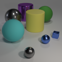
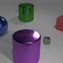
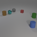
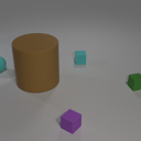
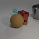
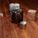
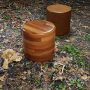
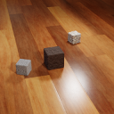
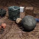
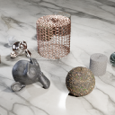
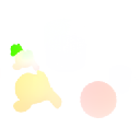
Figure 1: Example images and optical flow of the MovingCLEVR and MovingClevrTex datasets, which extend CLEVR and ClevrTex respectively to short videos based on physics simulation. Note that only a subset of objects is in motion in each frame.

To evaluate our method on still images, we use CLEVR [25] and ClevrTex [27] benchmark suites. Both consist of images depicting 3–10 objects. CLEVR images are simpler with uniformly colored objects with metallic or rubbery materials. ClevrTex features more diverse objects with complex textures applied. We also use the OOD and CAMO test sets from ClevrTex benchmark. OOD contains out-of-distribution shapes and textures. CAMO has camouflaged objects where the same texture is sampled for objects and the background.

Since our method requires optical flow during training, we extend the implementation of [27] to generate video datasets of CLEVR and ClevrTex scenes, where a subset of objects contained in each scene are sliding, rolling and colliding based on a physics simulation (Fig. 1). We generate 10k sequences for MovingClevrTex and 5k for MovingCLEVR, where we retain 1000 and 500 sequences, respectively, for validation. Each sequence is 5 frames long. Dataset details can be found in the Appendix. The evaluation is performed on the original CLEVR and ClevrTex test sets.

We also evaluate our method on the real-world KITTI [16] benchmark which depicts street scenes captured from a moving car. We follow the set up of [3], using 147 videos for training and evaluate on the instance segmentation subset which contains 200 annotated validation frames.

Metrics.

Following prior work [28, 27], we measure performance using two metrics. FG-ARI is the Adjusted Rand Index measured on foreground pixels only (selected using the ground-truth segmentation). Mean Intersection-over-Union (mIoU), is measured through Hungarian matching and averaged across the number of predicted or ground truth components, whichever is higher. When evaluating on videos, we calculate these metrics per-frame.

Network architecture.

Our method can employ any image segmentation network architecture and train from scratch. Unless otherwise specified, we use Mask2Former [6], using only its semantic segmentation. Following prior work [37, 28], we use a 6-layer CNN backbone on synthetic datasets and ResNet-18 for KITTI. We also experiment with Swin-tiny transformer [36] as the backbone. We use 11 transformer queries which become $K=11$ slots on CLEVR, ClevrTex, and MOVi-A/C. On MOVi-D/E, we set $K=24$ and $K=22$ on KITTI. The model takes approximately 48h to train on a single A30 24GB GPU. All training details and hyper-parameters are included in the Appendix.

4.2 Unsupervised multi-object segmentation in images

Table 1: Benchmark results on CLEVR, ClevrTex, CAMO, and OOD comparing FG-ARI and mIoU metrics (see also Appendix for an extended version). Results are a mean of 3 seeds $(\pm\sigma)$. Methods above the line are trained on single images, while methods below train on videos.^† – indicates post-processing.

	CLEVR		ClevrTex		OOD		CAMO
Model	FG-ARI$\uparrow$	mIoU$\uparrow$	FG-ARI$\uparrow$	mIoU$\uparrow$	FG-ARI$\uparrow$	mIoU$\uparrow$	FG-ARI$\uparrow$	mIoU$\uparrow$
SPAIR [9]	$77.13$$\pm$$1.92$	$65.95$$\pm$$4.02$	$0.00$$\pm$$0.00$	$0.00$$\pm$$0.00$	$0.00$$\pm$$0.00$	$0.00$$\pm$$0.00$	$0.00$$\pm$$0.00$	$0.00$$\pm$$0.00$
SPAIR†	$77.05$$\pm$$1.96$	$66.87$$\pm$$9.65$	$0.00$$\pm$$0.00$	$0.00$$\pm$$0.00$	$0.00$$\pm$$0.00$	$0.00$$\pm$$0.00$	$0.00$$\pm$$0.00$	$0.00$$\pm$$0.00$
MN [47]	$72.12$$\pm$$0.64$	$56.81$$\pm$$0.40$	$38.31$$\pm$$0.70$	$10.46$$\pm$$0.10$	$37.29$$\pm$$1.04$	$12.13$$\pm$$0.19$	$31.52$$\pm$$0.87$	$8.79$$\pm$$0.15$
MN†	$72.08$$\pm$$0.62$	$57.61$$\pm$$0.40$	$38.34$$\pm$$0.73$	$10.34$$\pm$$0.12$	$37.28$$\pm$$1.07$	$11.97$$\pm$$0.21$	$31.54$$\pm$$0.87$	$8.77$$\pm$$0.18$
MONet [5]	$54.47$$\pm$$11.41$	$30.66$$\pm$$14.87$	$36.66$$\pm$$0.87$	$19.78$$\pm$$1.02$	$32.97$$\pm$$1.00$	$19.30$$\pm$$0.37$	$12.44$$\pm$$0.73$	$10.52$$\pm$$0.38$
MONet†	$61.36$$\pm$$7.33$	$45.61$$\pm$$4.80$	$35.64$$\pm$$1.17$	$23.59$$\pm$$0.29$	$31.51$$\pm$$1.46$	$23.04$$\pm$$0.52$	$9.94$$\pm$$0.50$	$11.31$$\pm$$0.30$
SA [37]	$95.89$$\pm$$2.37$	$36.61$$\pm$$24.83$	$62.40$$\pm$$2.23$	$22.58$$\pm$$2.07$	$58.45$$\pm$$1.87$	$20.98$$\pm$$1.59$	$57.54$$\pm$$1.01$	$19.83$$\pm$$1.41$
SA†	$94.88$$\pm$$1.67$	$37.68$$\pm$$26.56$	$61.60$$\pm$$2.29$	$21.96$$\pm$$1.79$	$57.41$$\pm$$1.92$	$20.60$$\pm$$1.45$	$56.85$$\pm$$1.12$	$19.42$$\pm$$1.42$
IODINE [19]	$93.81$$\pm$$0.76$	$45.14$$\pm$$17.85$	$59.52$$\pm$$2.20$	$29.17$$\pm$$0.75$	$53.20$$\pm$$2.55$	$26.28$$\pm$$0.85$	$36.31$$\pm$$2.57$	$17.52$$\pm$$0.75$
IODINE†	$93.68$$\pm$$0.83$	$44.20$$\pm$$18.67$	$60.63$$\pm$$2.50$	$29.40$$\pm$$1.10$	$54.92$$\pm$$2.24$	$27.96$$\pm$$0.81$	$38.29$$\pm$$1.40$	$18.87$$\pm$$0.52$
DTI-S [43]	$89.54$$\pm$$1.44$	$48.74$$\pm$$2.17$	$79.90$$\pm$$1.37$	$33.79$$\pm$$1.30$	$73.67$$\pm$$0.98$	$32.55$$\pm$$1.08$	$72.90$$\pm$$1.89$	$27.54$$\pm$$1.55$
DTI-S†	$89.86$$\pm$$1.78$	$53.38$$\pm$$3.51$	$79.86$$\pm$$1.36$	$32.20$$\pm$$1.49$	$73.60$$\pm$$0.97$	$30.74$$\pm$$1.22$	$72.89$$\pm$$1.88$	$26.30$$\pm$$1.57$
GNM [23]	$65.05$$\pm$$4.19$	$59.92$$\pm$$3.72$	$53.37$$\pm$$0.67$	$42.25$$\pm$$0.18$	$48.43$$\pm$$0.86$	$40.84$$\pm$$0.30$	$15.73$$\pm$$0.89$	$17.56$$\pm$$0.74$
GNM†	$65.67$$\pm$$4.23$	$63.38$$\pm$$3.76$	$53.38$$\pm$$0.67$	$44.30$$\pm$$0.19$	$48.44$$\pm$$0.86$	$42.87$$\pm$$0.28$	$15.72$$\pm$$0.89$	$18.53$$\pm$$0.75$
SAVi [28]	—	—	$49.54$	$31.88$	$42.68$	$30.31$	$42.67$	$29.60$
Ours	$91.69$$\pm$$0.30$	$66.70$$\pm$$0.32$	$90.80$$\pm$$0.22$	$55.07$$\pm$$0.44$	$76.01$$\pm$$0.56$	$46.84$$\pm$$0.20$	$72.78$$\pm$$1.31$	$42.30$$\pm$$1.09$
Ours †	95.94$\pm$$0.43$	84.86$\pm$$4.06$	92.61$\pm$$0.22$	77.67$\pm$$0.25$	78.24$\pm$$0.43$	55.54$\pm$$0.44$	77.43$\pm$$0.86$	56.43$\pm$$0.80$

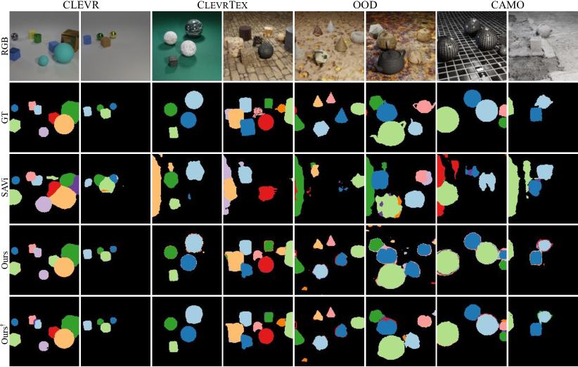
Figure 2: Unsupervised object segmentation on CLEVR and ClevrTex benchmarks. Our model is able to segment simple and visually complex scenes. Occasional mistakes around object boundaries and the assignment of different objects to the same component are addressed by post-processing. ^† – indicates post-processing.

In Table 1, we evaluate our method on the CLEVR [25] and ClevrTex [27] benchmarks and compare to prior work. Our method outperforms image models based on appearance reconstruction on both metrics (mIoU and FG-ARI) and across all datasets. The performance gap increases on the visually complex ClevrTex, OOD, and CAMO variants, demonstrating the strong inductive bias that motion provides during training, especially when the objects are camouflaged. Note that, in this setting, our model is advantaged compared to the other models in Table 1, as it can observe (through the loss) the optical flow of the training scenes. For this reason, we also train the optical flow-based, unconditional SAVi [28] model. Nevertheless, we find that despite having access to motion information during training, SAVi does not surpass appearance-only models, likely due to only having access to single frames at test time.

Post-processing helps improve results further. As shown in Fig. 2, separating connected components in post-processing distinguishes objects that might be assigned to the same mask and suppresses boundary segments that tend to group difficult occlusion boundaries. For a fairer comparison, we also test if this post-processing improves the results of other methods but only obtain mixed results.

4.3 Unsupervised multi-object segmentation in video

Table 2: Segmentation results on MOVi datasets. Mean $\pm$ standard error (5 seeds). We calculate metric for each frame. All values in $\%$. (WL) marks use of warp loss. ^† – indicates post-processing.

	MOVi-A		MOVi-C		MOVi-D		MOVi-E
Model	FG-ARI$\uparrow$	mIoU$\uparrow$	FG-ARI$\uparrow$	mIoU$\uparrow$	FG-ARI$\uparrow$	mIoU$\uparrow$	FG-ARI$\uparrow$	mIoU$\uparrow$
GWM [8]	$70.30$	$42.27$	$49.98$	$30.17$	$39.78$	$18.38$	$42.50$	$18.74$
SCALOR [24]	$59.57$	$44.41$	$40.43$	$22.54$	–	–	–	–
SAVi [28]	$\mathbf{88.30}$	$62.69$	$43.26$	$31.92$	$43.45$	$10.60$	$17.39$	$5.75$
Ours	$84.01$$\pm$$0.72$	$60.08$$\pm$$1.47$	$61.18$$\pm$$0.84$	$34.72$$\pm$$0.17$	55.74$\pm$$1.02$	$23.50$$\pm$$0.35$	$62.62$$\pm$$0.92$	$25.78$$\pm$$0.27$
Ours†	$85.41$$\pm$$1.00$	76.19$\pm$$2.05$	61.24$\pm$$0.85$	37.26$\pm$$0.33$	$55.18$$\pm$$0.94$	25.21$\pm$$0.29$	63.11$\pm$$0.91$	28.59$\pm$$0.29$
Ours† (Swin + WL)	$90.08$	$84.76$	$67.64$	$52.17$	$66.41$	$30.40$	$72.73$	$35.30$

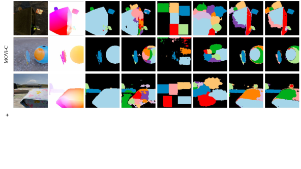
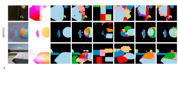
Figure 3: Qualitative comparisons on MOVi-A and MOVi-C. Our method performs consistently well compared to other methods. GWM suffers from oversegmentation where SCALOR has undersegmentation issue. Among the related methods, SCALOR fails to discover all the objects and SAVi’s object boundaries are coarser ^†– indicates post-processing.

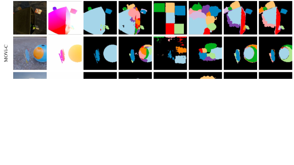
Figure 4: Failure cases on MOVi-A and MOVi-C. Our method has difficulty with objects that typically exhibit complex motion. It results in an over-segmentation of the object. Due to inherently imprecise optical flow near the boundaries our method also has a tendency to segment boundary pixels into a separate mask, which we fix with our post-processing step. ^†– indicates post-processing.

We now evaluate our approach on video segmentation, where motion is available at test time. We report the performance of our method in Table 2 compared to video-based models: SCALOR [24], unconditional SAVi [28], and GWM [8]; the latter two also use optical flow supervision. It is important to note that SAVi and SCALOR make predictions jointly over all frames of a video, that allows them to actually see the objects in motion at test time. Despite this comparison being unfair to our approach, which operates on a single frame at a time, we achieve competitive results. On the visually simpler MOVi-A, our method has more than 10% lead over SAVi in mIoU, but performs slightly worse in terms of FG-ARI. On the more complex MoVi-C/D/E datasets our model shows strong performance, outperforming prior work on both metrics, with the performance gap again increasing with data complexity. Finally, we experiment with a version of the model using a deeper backbone (Swin) and the warp loss (Eq. 8). Though not necessary to achieve state-of-art results, this drastically improves performance on all metrics and dataset versions. In Fig. 3, we also compare these models qualitatively, demonstrating that the different objects are overall better captured by our model with more refined boundaries, which explains the higher mIoU.

4.4 Model ablations

Optical flow.

In Table 3(a), we replace the ground-truth optical flow used so far in our experiments with the one estimated by SMURF [49]. The additional noise impacts our model’s accuracy, as evidenced by the significant drop in mIoU (but comparable FG-ARI scores).

Motion model.

In Table 3(b), we compare our affine motion model to the simpler translation-only one. We observe that the ability to describe complex motion patterns with an affine model improves performance over the translation model, which can only represent translation in the camera plane.

Table 3: Model ablations. (3(a)) replacing flow supervision with an unsupervised flow method, (3(b)) compares a translation-only with the affine flow model, and (3(c)) adds our motion-based formulation to an appearance-only model. All models with post-processing applied.

(a) Choice of Optical Flow Method

	MOVi-A		MOVi-C
Optical Flow	FG-ARI$\uparrow$	mIoU$\uparrow$	FG-ARI$\uparrow$	mIoU$\uparrow$
SMURF [49]	$80.17$	$26.3$	$61.21$	$28.77$
Ground Truth	$83.48$	$72.61$	$58.59$	$35.67$

(b) Choice of Motion Model

	MOVi-A		MOVi-C
Motion Mdl.	FG-ARI$\uparrow$	mIoU$\uparrow$	FG-ARI$\uparrow$	mIoU$\uparrow$
Translation	$66.03$	$59.94$	$39.77$	$32.23$
Affine	$83.48$	$72.61$	$58.59$	$35.67$

(c) Adding motion awareness to appearance-only models

		ClevrTex		OOD		CAMO
Model	Train data	FG-ARI$\uparrow$	mIoU$\uparrow$	FG-ARI$\uparrow$	mIoU$\uparrow$	FG-ARI$\uparrow$	mIoU$\uparrow$
GNM [23]	ClevrTex	$53.38$	$44.30$	$48.44$	$42.87$	$15.72$	$18.53$
GNM [23]	MovingClevrTex	$18.01$	$31.47$	$15.57$	$15.57$	$0.21$	$14.68$
GNM+Our Loss	MovingClevrTex	$63.84$	$55.26$	$59.01$	$48.65$	$51.00$	$47.63$
SA [37]	ClevrTex	$62.40$	$22.58$	$58.45$	$20.98$	$57.54$	$19.83$
SA [37]	MovingClevrTex	$61.84$	$21.44$	$58.24$	$20.67$	$57.30$	$18.82$
SA+Our Loss	MovingClevrTex	$76.60$	$38.12$	$67.01$	$33.95$	$70.59$	$33.05$

Motion awareness.

Finally, we investigate the effectiveness of our objective in combination with existing appearance-based methods. The goal of this experiment is to understand the advantage of using motion information during training (if available) and to decouple the effect of our formulation from the choice of architecture. To this end, we employ our objective on top of two models based on appearance reconstruction, GNM [23] and SA [37], with no other modifications. We train GNM and SA with and without our loss on videos (MovingClevrTex) and evaluate on the corresponding single-image test sets of the ClevrTex suite. In Table 3(c), we compare these models respectively to the original methods trained on static images (ClevrTex). We find that when trained on video data (MovingClevrTex), without our loss, both GNM and SA struggle. We attribute this to the reduced number of scenes in MovingClevrTex compared to ClevrTex. However, we note that using our loss significantly improves the performance of the appearance methods, suggesting the effectiveness of exploiting motion information through our formulation.

4.5 Segmentation on real-world data

Table 4: Real-world segmentation results on KITTI. Baseline results from [3]. Bao et al. [3] and our method use RAFT for optical flow. Models above the line use ResNet-18 backbone. (WL) marks use of warp loss.

	KITTI
Model	FG-ARI$\uparrow$
SA [37]	$13.8$
MONet [5]	$14.9$
SCALOR [35]	$21.1$
S-IODINE [19]	$14.4$
MCG [2]	$40.9$
Bao et al. [3]	$47.1$
Ours	$50.8$
Ours (WL)	$\mathbf{51.9}$
Ours (Swin + WL)	$58.3$

We now turn to assessing our model’s performance in a real-world setting. We follow the setting of Bao et al. [3] and evaluate on KITTI [16], using RAFT [50] to estimate optical flow and ResNet-18 as the backbone of our model, trained from scratch. We lower the input resolution for our model from $368\times 1,248$ [3] to $288\times 960$, which enables us to fit on a single GPU. We evaluate at $96\times 320$ resolution.

As we show in Table 4, our method outperforms prior work on the challenging real-world setting. In the same table, we also consider our method with an additional warp loss term, which further boosts performance. We also experiment with a transformer-based backbone (Swin) which is also pre-trained using self-supervision. Although, not necessary to show state-of-art result, this significantly improves real-world performance.

4.6 Limitations

Motion is sometimes insufficient to distinguish different objects, for instance because they do not move or because they move similarly. In principle, this should not matter if sufficient motion diversity is observed in the training data as a whole; in practice, our model occasionally merges different object at test time, which we address partly in post-processing. Further improvements could be obtained by choosing a more informative prior $p_{0}(\mathbf{m})$ in Eq. 1, to capture other desirable properties of objects, such as compactness and connectedness.

Figure 4 shows some failure cases where the affine motion model struggles to capture strong perspective effects caused by non-smooth depth changes in the object geometry. This could be addressed by modeling the object geometry (depth) and the ensuing complex flow patterns. Alternatively, this could be dealt with using a hierarchical segmentation model that can account for geometric discontinuities and self-occlusions. Hierarchical segmentation would also help with pronounced non-rigid motion (e.g. humans dancing or animals running) as motion could be explained at the level of object parts.

5 Conclusions

We have presented a method that bridges the gap between image-based and video-based scene decomposition, in that it requires only a single image as input, yet exploits motion cues available in videos during training. In comparison to prior work on image-based multi-object segmentation, our approach shows that motion provides useful objectness cues, especially as the visual complexity of a scene increases. Different from video-based approaches, however, our model operates on still images and does not rely on motion to detect or refine objects, which makes it more generally applicable. Finally, we deviate from the common objective of image or flow reconstruction and, instead, model the problem by only predicting regions likely to contain affine flow patterns. This does not require a specialized architecture, thus any segmentation network is suitable for this task. Our approach achieves state-of-the-art performance on multiple image and video benchmarks, in simulated and real-world settings, validating the paradigm of training image models using motion.

Broader impact.

Our work introduces a principled method for unsupervised multi-object segmentation. The work is mainly evaluated on 3D simulated datasets that do not contain people or personal information. Additionally, we evaluate on KITTI, a real-world self-driving dataset, which occasionally contains images of pedestrians. Consent cannot be obtained in this case, but we follow the KITTI terms of usage. We build on top of open source projects, respecting licenses and release all code, trained models and datasets for research purposes. Currently, the application of this approach is mainly limited to simulated imagery. Although the results on KITTI show promise, the immediate broader impact of our work in real-world scenarios, beyond the research community, is limited.

Acknowledgements

L. K. is funded by EPSRC Centre for Doctoral Training in Autonomous Intelligent Machines and Systems EP/S024050/1. S. C. is supported by a scholarship sponsored by Facebook. I. L., C. R. and A. V. are supported by European Research Council (ERC) grant 2020-CoG-101001212 UNION. I. L. and C. R. are also funded by EPSRC grant VisualAI EP/T028572/1.

Checklist

1. For all authors…

   1. Do the main claims made in the abstract and introduction accurately reflect the paper’s contributions and scope? [Yes]

   2. Did you describe the limitations of your work? [Yes] See Section 4.6.

   3. Did you discuss any potential negative societal impacts of your work? [Yes] See Section 5

   4. Have you read the ethics review guidelines and ensured that your paper conforms to them? [Yes]

2. If you are including theoretical results…

   1. Did you state the full set of assumptions of all theoretical results? [Yes]

   2. Did you include complete proofs of all theoretical results? [Yes] Longer form derivations are included in the supplementary material.

3. If you ran experiments…

   1. Did you include the code, data, and instructions needed to reproduce the main experimental results (either in the supplemental material or as a URL)? [Yes] We include instruction and specification of our methods. See project page https://www.robots.ox.ac.uk/~vgg/research/ppmp for code and checkpoints.

   2. Did you specify all the training details (e.g., data splits, hyperparameters, how they were chosen)? [Yes] See supplementary material

   3. Did you report error bars (e.g., with respect to the random seed after running experiments multiple times)? [Yes] See e.g. Table 1 and Table 2

   4. Did you include the total amount of compute and the type of resources used (e.g., type of GPUs, internal cluster, or cloud provider)? [Yes] See Section 4.1

4. If you are using existing assets (e.g., code, data, models) or curating/releasing new assets…

   1. If your work uses existing assets, did you cite the creators? [Yes] See Section 4.1

   2. Did you mention the license of the assets? [Yes]

   3. Did you include any new assets either in the supplemental material or as a URL? [Yes] We provide the code for dataset creation and examples of the dataset in the supplementary material (due to size). See project page https://www.robots.ox.ac.uk/~vgg/research/ppmp for data.

   4. Did you discuss whether and how consent was obtained from people whose data you’re using/curating? [Yes] We include one experiment on the KITTI dataset following their terms of usage. This data contains accidentally-captured pedestrians, from which consent cannot be obtained. These are ignored in the evaluation.

   5. Did you discuss whether the data you are using/curating contains personally identifiable information or offensive content? [Yes] See Section 5.

5. If you used crowdsourcing or conducted research with human subjects…

   1. Did you include the full text of instructions given to participants and screenshots, if applicable? [N/A]

   2. Did you describe any potential participant risks, with links to Institutional Review Board (IRB) approvals, if applicable? [N/A]

   3. Did you include the estimated hourly wage paid to participants and the total amount spent on participant compensation? [N/A]

Supplementary Material

In this supplementary material, we provide additional details for our loss function (Appendix A), including detailed derivation steps, implementation details, and further discussion of the advantages. Appendix C specifies hyperparameters used and how they were selected. We conclude with additional ablation experiments (Appendix D) and results (Appendix E). Project page and code: https://www.robots.ox.ac.uk/~vgg/research/ppmp.

Appendix A Loss derivation

The key part of our loss function is the likelihood of the optical flow $p(\mathbf{f}\mid\mathbf{m})$, which serves to evaluate how probable is a region of the optical flow carved out by the predicted masks for K regions. We assume that optical flow within a region depends only on the region itself and that other regions have no influence. Intuitively, this is a reasonable assumption, as in large, the movement/flow of an object does not depend on the background or other objects. Thus, enforcing this assumption encourages regions to correspond to objects.

The assessment of probability of optical flow within the region is based on the assumption that objects should be moving rigidly. We use an approximate parametric motion model (Eq. (2)). The parameters of the motion model $\theta$ abstract away unknown aspects such as scene geometry and camera intrinsics but enable to translate between assumed 3D rigid motion and 2D optical flow.

We assume that motion parameters $\theta_{k}\sim\mathcal{N}(\theta;\mu,\Sigma)$ come from a multivariate Gaussian prior. This choice enables expressing marginal-likelihood in closed-form.

We model the error of the approximate motion model as zero-mean isotropic Gaussian noise $\epsilon\sim\mathcal{N}(\epsilon;0,\sigma^{2}I)$.

Following the motion model (Eq. (2)), the optical flow $\mathbf{f}_{k}$ is an affine combination of Gaussian random variables. Using this observation, its distribution is

$$p(\mathbf{f}_{k}\mid\mathbf{m}_{k})=\det(2\pi(P_{k}\Sigma P_{k}^{\top}+\sigma^{2}I))^{-\nicefrac{{1}}{{2}}}\cdot\exp(-\frac{1}{2}\mathbf{F}_{k}^{\top}(P_{k}\Sigma P_{k}^{\top}+\sigma^{2}I)^{-1}\mathbf{F}_{k}),$$ (9)

where $\mathbf{F}_{k}=\mathbf{f}_{k}-\Pi_{\mu}(\Omega_{k})+\Omega_{k}$ is the centered flow within the region $k$. This equation can be slightly simplified by considering its two troublesome parts, the determinant and the quadratic form inside the exponent. For the determinant, we note the following:

$$\det(2\pi P_{k}\Sigma P_{k}^{\top}+2\pi\sigma^{2}I) =(2\pi\sigma^{2})^{2n_{k}}\det(\nicefrac{{1}}{{\sigma^{2}}}P_{k}\Sigma P_{k}^{\top}+I)$$

$$=(2\pi\sigma^{2})^{2n_{k}}\det(\Sigma)\det(\nicefrac{{1}}{{\sigma^{2}}}P_{k}^{\top}P_{k}+\Sigma^{-1})$$ (*)

$$=\frac{(2\pi\sigma^{2})^{2n_{k}}}{\det(\Lambda)}\det(\underbrace{\nicefrac{{1}}{{\sigma^{2}}}P_{k}^{\top}P_{k}+\Lambda}_{S_{k}}),$$

where in the line marked with (*) we apply matrix determinant lemma, and in the last line we substitute covariance $\Sigma^{-1}=\Lambda$ for the precision matrix. Similarly, the quadratic form in the exponent can be expanded

$$\mathbf{F}_{k}^{\top}(P_{k}\Sigma P_{k}^{\top}+\sigma^{2}I)^{-1}\mathbf{F}_{k} =\nicefrac{{1}}{{\sigma^{2}}}\mathbf{F}_{k}^{\top}(\nicefrac{{1}}{{\sigma^{2}}}P_{k}\Sigma P_{k}^{\top}+I)^{-1}\mathbf{F}_{k}$$

$$=\nicefrac{{1}}{{\sigma^{2}}}\mathbf{F}_{k}^{\top}\left(I-\nicefrac{{1}}{{\sigma^{2}}}P_{k}(\nicefrac{{1}}{{\sigma^{2}}}P_{k}^{\top}P_{k}+\Lambda)^{-1}P_{k}^{\top}\right)\mathbf{F}_{k} \dagger$$ ()

$$=\nicefrac{{1}}{{\sigma^{2}}}\mathbf{F}_{k}^{\top}\mathbf{F}_{k}-(\nicefrac{{1}}{{\sigma^{2}}})^{2}\mathbf{F}_{k}^{\top}P_{k}(\underbrace{\nicefrac{{1}}{{\sigma^{2}}}P_{k}^{\top}P_{k}+\Lambda}_{S_{k}})^{-1}P_{k}^{\top}\mathbf{F}_{k},$$

where in the line marked with ($\dagger$) the Woodbury identity is applied. The optical flow for the whole image is modeled as a joint of independent flow regions $\mathbf{f}_{k}$, giving the log-likelihood as

$$\log p(\mathbf{f}\mid\mathbf{m})=\sum_{k}\log p(\mathbf{f}_{k}\mid\mathbf{m}_{k})$$

$$=-\frac{1}{2}\left(2\log(2\pi\sigma^{2})\sum_{k}n_{k}+\sum_{k}\log\frac{\det S_{k}}{\det\Lambda}+\nicefrac{{1}}{{\sigma^{2}}}\sum_{k}\mathbf{F}_{k}^{\top}\mathbf{F}_{k}-(\nicefrac{{1}}{{\sigma^{2}}})^{2}\sum_{k}\mathbf{F}_{k}^{\top}P_{k}S_{k}^{-1}P_{k}^{\top}\mathbf{F}_{k}\right)$$

$$=-\frac{1}{2}\left(2\log(2\pi\sigma^{2})n+\sum_{k}\log\frac{\det S_{k}}{\det\Lambda}+\nicefrac{{1}}{{\sigma^{2}}}\mathbf{F}^{\top}\mathbf{F}-(\nicefrac{{1}}{{\sigma^{2}}})^{2}\sum_{k}\mathbf{F}^{\top}L_{k}PS_{k}^{-1}P^{\top}L_{k}\mathbf{F}\right),$$ (10)

where in the last line we introduced $n=\sum_{k}n_{k}=HW$, the number of pixels in the image. We also use product of selector matrices $L_{k}=R_{k}^{\top}R_{k}=\operatorname{diag}(\mathbf{m}_{k},\mathbf{m}_{k})=L_{k}^{\top}$ such that $\mathbf{F}_{k}^{\top}P_{k}=\mathbf{F}^{\top}L_{k}P$. This explicitly includes masks in the expression. Finally, we use the fact that regions partition the full image $\sum_{k}\mathbf{F}_{k}^{\top}\mathbf{F}_{k}=\sum_{k}\sum_{i}(\mathbf{F}_{k})_{i}^{2}=\mathbf{F}^{\top}\mathbf{F}$. We now manipulate Appendix A using specific details of the motion model to arrive at expressions that are convenient to implement in code.

A.1 Implementation details

Translation-only likelihood

We assume that translation along x and y directions is independent, such that $\theta$ prior is a zero-mean Gaussian with isotropic covariance $\tau^{2}I$. $P_{k}^{\mathrm{tr}}=\operatorname{diag}(\mathbf{1}_{n_{k}},\mathbf{1}_{n_{k}})$ and by extension $P^{\mathrm{tr}}=\operatorname{diag}(\mathbf{1}_{n},\mathbf{1}_{n})$. The matrix $S_{k}$ simplifies to

$$S_{k}=\nicefrac{{1}}{{\sigma^{2}}}P_{k}^{\top}P_{k}+\Lambda=\nicefrac{{1}}{{\sigma^{2}}}\begin{pmatrix}\mathbf{1}_{n_{k}}^{\top}\mathbf{1}_{n_{k}}&0\\ 0&\mathbf{1}_{n_{k}}^{\top}\mathbf{1}_{n_{k}}\end{pmatrix}+\nicefrac{{1}}{{\tau^{2}}}I=\nicefrac{{1}}{{\sigma^{2}}}(n_{k}+\nicefrac{{\sigma^{2}}}{{\tau^{2}}})I\,,$$

such that

$$\det S_{k}=(\nicefrac{{1}}{{\sigma^{2}}}(n_{k}+\nicefrac{{\sigma^{2}}}{{\tau^{2}}}))^{2},\quad\log\frac{\det S_{k}}{\det{\Lambda}}=2\log\frac{n_{k}+\nicefrac{{\sigma^{2}}}{{\tau^{2}}}}{\nicefrac{{\sigma^{2}}}{{\tau^{2}}}},\quad S_{k}^{-1}=(\nicefrac{{1}}{{\sigma^{2}}}(n_{k}+\nicefrac{{\sigma^{2}}}{{\tau^{2}}}))^{-1}I.$$

Writing $\mathbf{F}^{\top}=(\mathbf{u}^{\top},\mathbf{v}^{\top})$ to denote x and y components of the flow, respectively, the term reduces

$$(\nicefrac{{1}}{{\sigma^{2}}})^{2}\sum_{k}\mathbf{F}^{\top}L_{k}PS_{k}^{-1}P^{\top}L_{k}\mathbf{F} =\nicefrac{{1}}{{\sigma^{2}}}\sum_{k}\mathbf{F}^{\top}L_{k}^{\top}PP^{\top}L_{k}\mathbf{F}\frac{1}{n_{k}+\nicefrac{{\sigma^{2}}}{{\tau^{2}}}}$$

$$=\nicefrac{{1}}{{\sigma^{2}}}\sum_{k}\frac{1}{n_{k}+\nicefrac{{\sigma^{2}}}{{\tau^{2}}}}\begin{bmatrix}\mathbf{u}^{\top}&\mathbf{v}^{\top}\\ \end{bmatrix}\begin{bmatrix}\mathbf{m}_{k}\mathbf{m}_{k}^{\top}&\\ &\mathbf{m}_{k}\mathbf{m}_{k}^{\top}\\ \end{bmatrix}\begin{bmatrix}\mathbf{u}\\ \mathbf{v}\\ \end{bmatrix}$$

$$=\nicefrac{{1}}{{\sigma^{2}}}\sum_{k}\frac{1}{n_{k}+\nicefrac{{\sigma^{2}}}{{\tau^{2}}}}\left((\mathbf{u}^{\top}\mathbf{m}_{k})^{2}+(\mathbf{v}^{\top}\mathbf{m}_{k})^{2}\right)$$

$$=\nicefrac{{1}}{{\sigma^{2}}}\sum_{k}\frac{n_{k}^{2}}{n_{k}+\nicefrac{{\sigma^{2}}}{{\tau^{2}}}}(\bar{u}_{k}^{2}+\bar{v}_{k}^{2})\,,$$

where in the last line we introduced mean flow $\bar{u}_{k}=n_{k}^{-1}\mathbf{u}^{\top}\mathbf{m}_{k}$ and $\bar{v}_{k}=n_{k}^{-1}\mathbf{v}^{\top}\mathbf{m}_{k}$. This gives the negative log-likelihood as

$$\log p(\mathbf{f}\mid\mathbf{m})=\sum_{k}\log p(\mathbf{f}_{k}\mid\mathbf{m}_{k})$$

$$=-\frac{1}{2}\left(2\log(2\pi\sigma^{2})n+\sum_{k}\log\frac{\det S_{k}}{\det\Lambda}+\nicefrac{{1}}{{\sigma^{2}}}\mathbf{F}^{\top}\mathbf{F}-(\nicefrac{{1}}{{\sigma^{2}}})^{2}\sum_{k}\mathbf{F}^{\top}L_{k}PS_{k}^{-1}P^{\top}L_{k}\mathbf{F}\right)$$

$$=-n\log(2\pi\sigma^{2})-\sum_{k}\log\frac{n_{k}+\nicefrac{{\sigma^{2}}}{{\tau^{2}}}}{\nicefrac{{\sigma^{2}}}{{\tau^{2}}}}-\frac{1}{2\sigma^{2}}\left(\mathbf{F}^{\top}\mathbf{F}-\sum_{k}\frac{n_{k}^{2}(\bar{u}_{k}^{2}+\bar{v}_{k}^{2})}{n_{k}+\nicefrac{{\sigma^{2}}}{{\tau^{2}}}}\right)$$

$$=-n\log(2\pi\sigma^{2})-\sum_{k}\log\frac{n_{k}+\nicefrac{{\sigma^{2}}}{{\tau^{2}}}}{\nicefrac{{\sigma^{2}}}{{\tau^{2}}}}-\frac{1}{2\sigma^{2}}\sum_{i=1}^{n}\left(u_{i}^{2}+v_{i}^{2}-\sum_{k}\frac{n_{k}(\bar{u}_{k}^{2}+\bar{v}_{k}^{2})}{n_{k}+\nicefrac{{\sigma^{2}}}{{\tau^{2}}}}(\mathbf{m}_{k})_{i}\right).$$ (11)

In our implementation, we extend this equation further. Writing $w_{k}=1-\sqrt{\frac{\nicefrac{{\sigma^{2}}}{{\tau^{2}}}}{n_{k}+\nicefrac{{\sigma^{2}}}{{\tau^{2}}}}}$, we note that the following sum is equivalent

$$\sum_{i=1}^{n}(u_{i}-\sum_{k}\bar{u}_{k}w_{k}(\mathbf{m}_{k})_{i})^{2} =\sum_{i=1}^{n}(u_{i}^{2}-\sum_{k}2u_{i}\bar{u}_{k}w_{k}(\mathbf{m}_{k})_{i}+\sum_{k}(\mathbf{m}_{k})_{i}w_{k}^{2}\bar{u}_{k}^{2})$$

$$=\sum_{i=1}^{n}u_{i}^{2}-\sum_{k}2\bar{u}_{k}w_{k}\sum_{i=1}^{n}u_{i}(\mathbf{m}_{k})_{i}+\sum_{k}w_{k}^{2}\bar{u}_{k}^{2}\sum_{i=1}^{n}(\mathbf{m}_{k})_{i}$$

$$=\sum_{i=1}^{n}u_{i}^{2}-\sum_{k}2\bar{u}_{k}^{2}w_{k}n_{k}+\sum_{k}w_{k}^{2}\bar{u}_{k}^{2}n_{k}$$

$$=\sum_{i=1}^{n}u_{i}^{2}-\sum_{k}\bar{u}_{k}^{2}n_{k}(2w_{k}-w_{k}^{2})$$

$$=\sum_{i=1}^{n}u_{i}^{2}-\sum_{k}\bar{u}_{k}^{2}\frac{n_{k}}{n_{k}+\nicefrac{{\sigma^{2}}}{{\tau^{2}}}}\sum_{i=1}^{n}(\mathbf{m}_{k})_{i}$$

$$=\sum_{i=1}^{n}\left(u_{i}^{2}-\sum_{k}\frac{n_{k}\bar{u}_{k}^{2}(\mathbf{m}_{k})_{i}}{n_{k}+\nicefrac{{\sigma^{2}}}{{\tau^{2}}}}\right),$$

where in the first line we make use of the fact that masks are one-hot $(\mathbf{m})_{i}\in\{0,1\}^{k}$, thus only a single term in the sums over $k$ is non-zero, i.e. $(\sum_{k}w_{k}\bar{u}_{k}(\mathbf{m}_{k})_{i})^{2}=\sum_{k}w_{k}^{2}\bar{u}_{k}^{2}(\mathbf{m}_{k})_{i})$. Using the above insight, the log-likelihood is

$$\log p(\mathbf{f}\mid\mathbf{m})=-n\log(2\pi\sigma^{2})-\sum_{k}\log\frac{n_{k}+\nicefrac{{\sigma^{2}}}{{\tau^{2}}}}{\nicefrac{{\sigma^{2}}}{{\tau^{2}}}}\\ -\frac{1}{2\sigma^{2}}\sum_{i=1}^{n}\left((u_{i}-\sum_{k}\bar{u}_{k}w_{k}(\mathbf{m}_{k})_{i})^{2}+(v_{i}-\sum_{k}\bar{v}_{k}w_{k}(\mathbf{m}_{k})_{i})^{2}\right)\,,$$ (12)

where

$$n_{k}=\sum_{i=1}^{n}(\mathbf{m}_{k})_{i}\,,\quad w_{k}=1-\sqrt{\frac{\nicefrac{{\sigma^{2}}}{{\tau^{2}}}}{n_{k}+\nicefrac{{\sigma^{2}}}{{\tau^{2}}}}}\,.$$

We then replace $\mathbf{m}$ with $\hat{\mathbf{m}}$ from the Gumbel-Softmax approximation.

Affine motion likelihood.

For the affine motion model, the full covariance matrix $\Sigma$ prevents significant further simplification. Instead, we transform the log-likelihood (Appendix A) to an equivalent form involving only $3\times 3$ matrices, for which the required determinant and inverse can be calculated analytically. To that end, we introduce the following auxiliary variables:

$$G_{k}=\begin{bmatrix}\mathbf{x}_{k}&\mathbf{y}_{k}&\mathbf{1}_{n_{k}}\end{bmatrix}\,,\quad P_{k}=\begin{bmatrix}G_{k}&0\\ 0&G_{k}\end{bmatrix}\,,\quad\Sigma^{-1}=\Lambda=\begin{bmatrix}\alpha&\beta\\ \gamma&\delta\end{bmatrix}\,.$$

Then $S_{k}$ is

$$S_{k}=\nicefrac{{1}}{{\sigma^{2}}}P_{k}^{\top}P_{k}+\Lambda=\begin{bmatrix}\nicefrac{{1}}{{\sigma^{2}}}G_{k}^{\top}G_{k}+\alpha&\beta\\ \gamma&\nicefrac{{1}}{{\sigma^{2}}}G_{k}^{\top}G_{k}+\delta\end{bmatrix}\,,$$

with

$$G_{k}^{\top}G_{k}=\begin{pmatrix}\mathbf{x}_{k}^{\top}\mathbf{x}_{k}&\mathbf{x}_{k}^{\top}\mathbf{y}_{k}&\mathbf{x}_{k}^{\top}\mathbf{1}_{n_{k}}\\ \mathbf{x}_{k}^{\top}\mathbf{y}_{k}&\mathbf{y}_{k}^{\top}\mathbf{y}_{k}&\mathbf{y}_{k}^{\top}\mathbf{1}_{n_{k}}\\ \mathbf{x}_{k}^{\top}\mathbf{1}_{n_{k}}&\mathbf{y}_{k}^{\top}\mathbf{1}_{n_{k}}&\mathbf{1}_{n_{k}}^{\top}\mathbf{1}_{n_{k}}\end{pmatrix}\,.$$

Using this, the determinant is

$$\det S_{k}=\det(\nicefrac{{1}}{{\sigma^{2}}}G_{k}^{\top}G_{k}+\alpha-\beta(\nicefrac{{1}}{{\sigma^{2}}}G_{k}^{\top}G_{k}+\delta)^{-1}\gamma)\det(\nicefrac{{1}}{{\sigma^{2}}}G_{k}^{\top}G_{k}+\delta).$$

Similarly, the inverse is then

$$S_{k}^{-1} =\begin{bmatrix}A_{k}&B_{k}\\ C_{k}&D_{k}\end{bmatrix}\,,\quad\textrm{where}$$

$$D_{k} =(\nicefrac{{1}}{{\sigma^{2}}}G_{k}^{\top}G_{k}+\delta-\gamma(\nicefrac{{1}}{{\sigma^{2}}}G_{k}^{\top}G_{k}+\alpha)^{-1}\beta)$$

$$C_{k} =-D_{k}\gamma(\nicefrac{{1}}{{\sigma^{2}}}G_{k}^{\top}G_{k}+\alpha)^{-1}$$

$$B_{k} =-(\nicefrac{{1}}{{\sigma^{2}}}G_{k}^{\top}G_{k}+\alpha)^{-1}\beta D_{k}$$

$$A_{k} =(\nicefrac{{1}}{{\sigma^{2}}}G_{k}^{\top}G_{k}+\alpha)^{-1}-B_{k}\gamma(\nicefrac{{1}}{{\sigma^{2}}}G_{k}^{\top}G_{k}+\alpha)^{-1}\mathrm{,~{}such~{}that}$$

$$\mathbf{h}_{k} =\begin{pmatrix}\mathbf{u}_{k}^{\top}\mathbf{x}_{k}&\mathbf{u}_{k}^{\top}\mathbf{y}_{k}&\mathbf{u}_{k}^{\top}\mathbf{1}_{n_{k}}\end{pmatrix}$$

$$\mathbf{r}_{k} =\begin{pmatrix}\mathbf{v}_{k}^{\top}\mathbf{x}_{k}&\mathbf{v}_{k}^{\top}\mathbf{y}_{k}&\mathbf{v}_{k}^{\top}\mathbf{1}_{n_{k}}\end{pmatrix}$$

$$\mathbf{F}_{k}^{\top}P_{k}S_{k}^{-1}P_{k}^{\top}\mathbf{F}_{k} =\mathbf{h}_{k}A_{k}\mathbf{r}_{k}^{\top}+\mathbf{r}_{k}C_{k}\mathbf{h}_{k}^{\top}+\mathbf{h}_{k}B_{k}\mathbf{r}_{k}^{\top}+\mathbf{r}_{k}D_{k}\mathbf{r}_{k}^{\top}.$$

We implement inner products under Gumbel-Softmax as $\mathbf{a}_{k}^{\top}\mathbf{b}_{k}=\sum_{i=1}^{n}(\mathbf{a})_{i}(\mathbf{b})_{i}(\hat{\mathbf{m}}_{k})_{i}$, for some vectors $\mathbf{a},\mathbf{b}$. The coordinate vectors $\mathbf{x}_{k},\mathbf{y}_{k}$ have the origin set to the centroid of the predicted region $\begin{pmatrix}x_{c,k}\\ y_{c,k}\end{pmatrix}=n_{k}^{-1}\begin{pmatrix}\mathbf{x}^{\top}\mathbf{m}_{k}\\ \mathbf{y}^{\top}\mathbf{m}_{k}\end{pmatrix}$. The expressions can then be substituted back to Appendix A. We show implementation in Algorithm 1.

Algorithm 1 Implementation of negative flow likelihood $-\log p(\mathbf{f}\mid\mathbf{m})$ under affine motion prior. Key quantities in the inner loop are underlined.

1:procedure NLL(mean $\mu$, covariance $\Sigma$, variance $\sigma^{2}$, flow $\mathbf{f}$, masks $\mathbf{m}_{k}$, height $H$, width $W$)

2:     $(\mu_{1}~{}\mu_{2}~{}\mu_{3}~{}\mu_{4}~{}\mu_{5}~{}\mu_{6})\leftarrow\mu$

3:     $\mathbf{x},\mathbf{y}\leftarrow\mathrm{lattice}(H,W)$

4:     $\begin{bmatrix}\mathbf{u}\\ \mathbf{v}\end{bmatrix}\leftarrow\mathbf{f}$

5:     $\Lambda\leftarrow\Sigma^{-1}$

6:     $\begin{bmatrix}\alpha&\beta\\ \gamma&\delta\end{bmatrix}\leftarrow\Lambda$

7:     for all $k$ regions do

8:         $n_{k}\leftarrow\sum_{i}(\mathbf{m}_{k})_{i}$

9:         $\mathbf{\hat{x}}_{k}\leftarrow\mathbf{x}-n_{k}^{-1}\mathbf{x}^{\top}\mathbf{m}_{k}$ $\triangleright$ Set origin to centroid

10:         $\mathbf{\hat{y}}_{k}\leftarrow\mathbf{y}-n_{k}^{-1}\mathbf{y}^{\top}\mathbf{m}_{k}$

11:         $\mathbf{x}_{k}^{\top}\mathbf{x}_{k}\leftarrow\sum_{i}(\mathbf{\hat{x}}_{k})_{i}^{2}(\mathbf{m}_{k})_{i}$

12:         $\mathbf{x}_{k}^{\top}\mathbf{y}_{k}\leftarrow\sum_{i}(\mathbf{\hat{x}}_{k})_{i}(\mathbf{\hat{y}}_{k})_{i}(\mathbf{m}_{k})_{i}$

13:         $\mathbf{y}_{k}^{\top}\mathbf{y}_{k}\leftarrow\sum_{i}(\mathbf{\hat{y}}_{k})_{i}^{2}(\mathbf{m}_{k})_{i}$

14:         $\mathbf{x}_{k}^{\top}\mathbf{1}_{n_{k}}\leftarrow\sum_{i}(\mathbf{\hat{x}}_{k})_{i}(\mathbf{m}_{k})_{i}$

15:         $\mathbf{y}_{k}^{\top}\mathbf{1}_{n_{k}}\leftarrow\sum_{i}(\mathbf{\hat{y}}_{k})_{i}(\mathbf{m}_{k})_{i}$

16:         $G_{k}^{\top}G_{k}\leftarrow\begin{pmatrix}\mathbf{x}_{k}^{\top}\mathbf{x}_{k}&\mathbf{x}_{k}^{\top}\mathbf{y}_{k}&\mathbf{x}_{k}^{\top}\mathbf{1}_{n_{k}}\\ \mathbf{x}_{k}^{\top}\mathbf{y}_{k}&\mathbf{y}_{k}^{\top}\mathbf{y}_{k}&\mathbf{y}_{k}^{\top}\mathbf{1}_{n_{k}}\\ \mathbf{x}_{k}^{\top}\mathbf{1}_{n_{k}}&\mathbf{y}_{k}^{\top}\mathbf{1}_{n_{k}}&n_{k}\end{pmatrix}$

17:         $D_{k}\leftarrow(\nicefrac{{1}}{{\sigma^{2}}}G_{k}^{\top}G_{k}+\delta-\gamma(\nicefrac{{1}}{{\sigma^{2}}}G_{k}^{\top}G_{k}+\alpha)^{-1}\beta)$

18:         $C_{k}\leftarrow-D_{k}\gamma(\nicefrac{{1}}{{\sigma^{2}}}G_{k}^{\top}G_{k}+\alpha)^{-1}$

19:         $B_{k}\leftarrow-(\nicefrac{{1}}{{\sigma^{2}}}G_{k}^{\top}G_{k}+\alpha)^{-1}\beta D_{k}$

20:         $A_{k}\leftarrow(\nicefrac{{1}}{{\sigma^{2}}}G_{k}^{\top}G_{k}+\alpha)^{-1}-B_{k}\gamma(\nicefrac{{1}}{{\sigma^{2}}}G_{k}^{\top}G_{k}+\alpha)^{-1}$

21:         $\mathbf{u}_{k}^{\top}\mathbf{x}_{k}\leftarrow\sum_{i}((\mathbf{u})_{i})((\mathbf{x})_{i}-x_{c,k})(\mathbf{m}_{k})_{i}$

22:         $\mathbf{\hat{u}}_{k}\leftarrow\mathbf{u}-((\mu_{1}-1)\mathbf{\hat{x}}+\mu_{2}\mathbf{\hat{y}}+\mu_{3})$ $\triangleright$ Center flow according to mean motion

23:         $\mathbf{\hat{v}}_{k}\leftarrow\mathbf{v}-((\mu_{5}-1)\mathbf{\hat{y}}+\mu_{4}\mathbf{\hat{x}}+\mu_{6})$

24:         $\underline{\mathbf{F}_{k}^{\top}\mathbf{F}_{k}}\leftarrow\sum_{i}(\mathbf{\hat{u}}_{k})_{i}^{2}(\mathbf{m}_{k})_{i}+\sum_{i}(\mathbf{\hat{v}}_{k})_{i}^{2}(\mathbf{m}_{k})_{i}$

25:         $\mathbf{u}_{k}^{\top}\mathbf{x}_{k}\leftarrow\sum_{i}(\mathbf{\hat{u}}_{k})_{i}(\mathbf{\hat{x}}_{k})_{i}(\mathbf{m}_{k})_{i}$

26:         $\mathbf{u}_{k}^{\top}\mathbf{y}_{k}\leftarrow\sum_{i}(\mathbf{\hat{u}}_{k})_{i}(\mathbf{\hat{y}}_{k})_{i}(\mathbf{m}_{k})_{i}$

27:         $\mathbf{u}_{k}^{\top}\mathbf{1}_{n_{k}}\leftarrow\sum_{i}(\mathbf{\hat{u}}_{k})_{i}(\mathbf{m}_{k})_{i}$

28:         $\mathbf{h}_{k}\leftarrow\begin{pmatrix}\mathbf{u}_{k}^{\top}\mathbf{x}_{k}&\mathbf{u}_{k}^{\top}\mathbf{y}_{k}&\mathbf{u}_{k}^{\top}\mathbf{1}_{n_{k}}\end{pmatrix}$

29:         $\mathbf{v}_{k}^{\top}\mathbf{x}_{k}\leftarrow\sum_{i}(\mathbf{\hat{v}}_{k})_{i}(\mathbf{\hat{x}}_{k})_{i}(\mathbf{m}_{k})_{i}$

30:         $\mathbf{v}_{k}^{\top}\mathbf{y}_{k}\leftarrow\sum_{i}(\mathbf{\hat{v}}_{k})_{i}(\mathbf{\hat{y}}_{k})_{i}(\mathbf{m}_{k})_{i}$

31:         $\mathbf{v}_{k}^{\top}\mathbf{1}_{n_{k}}\leftarrow\sum_{i}(\mathbf{\hat{v}}_{k})_{i}(\mathbf{m}_{k})_{i}$

32:         $\mathbf{r}_{k}\leftarrow\begin{pmatrix}\mathbf{v}_{k}^{\top}\mathbf{x}_{k}&\mathbf{v}_{k}^{\top}\mathbf{y}_{k}&\mathbf{v}_{k}^{\top}\mathbf{1}_{n_{k}}\end{pmatrix}$

33:         $\underline{\mathbf{F}_{k}^{\top}P_{k}S_{k}^{-1}P_{k}^{\top}\mathbf{F}_{k}}\leftarrow\mathbf{h}_{k}A_{k}\mathbf{r}_{k}^{\top}+\mathbf{r}_{k}C_{k}\mathbf{h}_{k}^{\top}+\mathbf{h}_{k}B_{k}\mathbf{r}_{k}^{\top}+\mathbf{r}_{k}D_{k}\mathbf{r}_{k}^{\top}$

34:         $\underline{\det S_{k}}\leftarrow\det(\nicefrac{{1}}{{\sigma^{2}}}G_{k}^{\top}G_{k}+\alpha-\beta(\nicefrac{{1}}{{\sigma^{2}}}G_{k}^{\top}G_{k}+\delta)^{-1}\gamma)\det(\nicefrac{{1}}{{\sigma^{2}}}G_{k}^{\top}G_{k}+\delta)$

35:     end for

36:     $\mathbf{return~{}~{}}HW\log(2\pi\sigma^{2})+\frac{1}{2}\sum_{k}\log\frac{\det S_{k}}{\det\Lambda}+\frac{1}{2\sigma^{2}}\sum_{k}(\mathbf{F}_{k}^{\top}\mathbf{F}_{k}-\mathbf{F}_{k}^{\top}P_{k}S_{k}^{-1}P_{k}^{\top}\mathbf{F}_{k})$

37:end procedure

A.2 Further justification

We consider whether the inclusion of the prior on the motion parameters offers any benefits. Consider a simple translation-only model. Since objects are only translating, each pixel in a region should be very close to the mean translation of that region. We can assess the mean for a region as $\begin{bmatrix}\bar{u}_{k}\mathbf{m}_{k}\\ \bar{v}_{k}\mathbf{m}_{k}\end{bmatrix}$, considering some variance $\sigma^{2}$ around it:

$$\log\hat{p}(\mathbf{f}\mid\mathbf{m}) =\log\mathcal{N}(\begin{bmatrix}\mathbf{u}\\ \mathbf{v}\end{bmatrix};\sum_{k}\begin{bmatrix}\bar{u}_{k}\mathbf{m}_{k}\\ \bar{v}_{k}\mathbf{m}_{k}\end{bmatrix},\sigma^{2}I)$$

$$=-n\log(2\pi\sigma^{2})-\frac{1}{2\sigma^{2}}\sum_{i=1}^{n}\left((u_{i}-\sum_{k}\bar{u}_{k}(\mathbf{m}_{k})_{i})^{2}+(v_{i}-\sum_{k}\bar{v}_{k}(\mathbf{m}_{k})_{i})^{2}\right).$$

Such model, up to a scaling factor, was already considered for features [7] and optical flow [8]. This expression for $\log\hat{p}(\mathbf{f}\mid\mathbf{m})$ can be compared with our version of translation only model Eq. 12. By considering the prior on the motion parameters, we introduce a weighing factor $w_{k}$ for each mean $\bar{u}_{k}\mathbf{m}_{k}$, which discounts the contribution of smaller segments. Similarly, the term $\sum_{k}\log\frac{n_{k}+\nicefrac{{\sigma^{2}}}{{\tau^{2}}}}{\nicefrac{{\sigma^{2}}}{{\tau^{2}}}}\approx\sum_{k}\log{n_{k}}$ encourages larger masks, since $\sum_{k}n_{k}=n$. The prior helps to encode that larger regions should be preferred.

Appendix B MovingClevrTex and MovingClevr

We extend the implementation of [27] to generate video datasets of CLEVR and ClevrTex scenes. We follow original sampling set up of ClevrTex – each scene contains a random arrangement of 3–10 objects. We uniformly choose between scenarios where a single random objects is given initial motion, two random objects are provided initial motion or all objects are moving. We sample a random initial translation in XY plane for the object between keyframes 0 and 3, which builds momentum. Physics simulation takes over from keyframe 4. Mass of each object is set to equal its scale (numerically), and we use value of 0.1 for the ‘bounciness’ parameters. This results in objects sliding, rotating due to shape and friction, and colliding. Collisions can make other objects move. Each simulation is 5 frames long and we render keyframes 4 to 8.

We sample 10000 scenes for MovingClevrTex, which gives the same number of frames as the original ClevrTex (where each scene had only single frame). For MovingClevr, we sample 5000 scenes. 1000 and 500 scenes are kept as validation for MovingClevrTex and for MovingClevr, respectively. We use the same rendering and lighting parameters as in  [27], except we slightly reduce the scale of the surface displacement mapping for the background. This reduces the visibility of clipping of the detailed object geometry with the background geometry, which might occur due to physics simulation working on simplified meshes.

Appendix C Hyperparameters

Our method can use any segmentation network $\Phi$. We employ the recent Mask2Former architecture, using 6-layer CNN backbone from [37, 28] for simulated datasets and ResNet-18 for KITTI in the main experiments. We also experiment with Swin-tiny transformer as the backbone, as it offers balanced performance in both visually simple and complex settings. We ablate these choices in Appendix D.

The networks are trained with AdamW [38], with a learning rate of $3\times 10^{-6}$ and batch size of 32, for 250k iterations. We employ gradient clipping when the 2-norm exceeds 0.01 and linear learning rate warm-up for the first 5k iterations to stabilize the training. The learning rate is reduced by a factor of 10 after 200k iterations. When training with warping loss on MOVi datasets, we found it beneficial to train for longer, for 500k iterations, reducing the learning rate by factor of 10 also after 400k iterations.

We found it beneficial to linearly anneal $\beta$ from 0.1 to -0.1 over 5k iterations, encouraging the network to explore initially but focus on low-entropy distributions in the end. We found this had the effect of encouraging the network to assign background pixels to a single slot.

For the prior, we set $\sigma^{2}$ (Appendix A) to $0.5$ and use $\mu=(1~{}0~{}0~{}0~{}1~{}0)^{\top}$. We use the following covariance matrix

$$\Sigma =\begin{pmatrix}0.005&0&0&0&0&0\\ 0&0.05&0&0&0&0\\ 0&0&15&0&0&0\\ 0&0&0&0.05&0&0\\ 0&0&0&0&0.005&0\\ 0&0&0&0&0&15\end{pmatrix}.$$

C.1 Settings in ablations

When experimenting with translation-only model, we use the same parameters and settings where possible. We set $\tau^{2}$, so $0.5,16.0,34.0$ for CLEVR/ClevrTex, MOVi-A, and MOVi-C, respectively (values picked from specialized covariance matrices, see Appendix D).

For GNM [23], we use implementation and parameters described in [27]. Owning to our loss being lower bound on log-probability, we simply add our loss to existing ELBO loss with hyperparameters above, only changing $\sigma^{2}=0.1$. We hypothesize that lower noise model is beneficial, as it provides stronger learning signal in the early stages when reconstruction is noisy due to untrained VAEs. The overfitting to errors of the motion approximation is handled, instead, by the networks balancing between appearance reconstruction and motion explanation objectives.

For SA [37], we also use implementation of [27]. SA loss is multiplied by 100 before adding our formulation.

C.2 Settings in KITTI

For experiments on KITTI, we replace the backbone to ResNet-18 to match prior work. We reduce batch size to 8, increase learning rate to $10^{-4}$. Learning rate is linearly warmed up for 10 iterations, and reduced by a factor of 10 after 5500 iterations. We employ backbone learning rate multiplier of 0.1. All other settings as before.

C.3 Model parameters of comparisons

Here we describe implementation and hyperparameters used for comparative methods in our experiments.

SAVi [28].

We follow the parameters given for conditional SAVi-S in their code repository, except to make SAVi unconditional we unset the conditioning key and make the slots to be learnable parameters.

SCALOR [24].

We use the optimized SCALOR parameters mentioned by SAVi [28] to train SCALOR. Particularly we use the MOVI dataset parameters to train MOVi-A and MOVI++ parameters to train MOVi-C.

GWM [8].

For GWM, we follow the parameters mentioned in the paper, except we do not employ spectral clustering and match the number of components to our settings for each dataset.

Appendix D Additional ablations

Table 5: Supplementary ablations for our methods. We show the impact segmentation networks have for different datasets Table 5(a). We further study the impact of our tuned covariance matrix in Table 5(b). Results with post-processing applied.

(a) Choice of Model Architecture

		MOVi-A		MOVi-C		MovingClevrTex
Architecture	# Params	FG-ARI$\uparrow$	mIoU$\uparrow$	FG-ARI$\uparrow$	mIoU$\uparrow$	FG-ARI$\uparrow$	mIoU$\uparrow$
M2F (Swin-tiny)	47M	$83.48$	$72.61$	$58.59$	$35.67$	$88.80$	$69.62$
M2F (ResNet50)	44M	$83.44$	$68.06$	$60.32$	$34.80$	$90.40$	$67.07$
M2F (ResNet18)	31M	$84.04$	$67.48$	$60.84$	$35.69$	$90.31$	$67.33$
MF (Swin-tiny)	44M	$81.78$	$71.28$	$54.45$	$33.67$	$71.07$	$51.06$
U-Net	31M	$90.79$	$82.85$	$60.28$	$26.62$	$87.03$	$39.66$

(b) Choice of Covariance Marix

	MOVi-A		MOVi-C
$\mathbf{\Sigma}$	FG-ARI$\uparrow$	mIoU$\uparrow$	FG-ARI$\uparrow$	mIoU$\uparrow$
Generic	$82.32$	$71.70$	$58.12$	$35.79$
Tuned	$83.48$	$72.61$	$58.59$	$35.67$

Segmentation network.

We study the effect of segmentation network in Table 5(a). We find that using a much simpler U-Net [45] architecture is beneficial on MOVi-A which contains visually plain scenes. The U-Net architecture, however, results in performance degradation on visually complex data.

We also consider a version of Mask2Former architecture that uses much deeper backbone, using Resnet-50 and Resnet-18, instead. We find that the deeper backbones leads to similar performance, indicating that our formulation is not architecture-specific. Finally, we change to MaskFormer architecture, matching the network architecture used in  [8], and use smaller Swin-tiny backbone. We find that our loss formulation leads to improved performance still.

Covariance matrix.

We investigate whether further improvements are possible using specialised versions of the prior. To that end, we offset the mean translation prior to account for the dominantly downward motion of objects on MOVi-A/MOVi-C. We use $\mu_{\mathrm{MOVi-A}}=(1~{}0~{}0~{}0~{}1~{}1.5)^{\top}$ and $\mu_{\mathrm{MOVi-C}}=(1~{}0~{}0~{}0~{}1~{}1.8)^{\top}$, respectively. We use the following specialized covariance matrices:

$$\Sigma_{\mathrm{MOVi-A}} =\begin{pmatrix}0.006&-0.00004&0&0.00004&0.001&0\\ -0.00004&0.04&0&-0.01&-0.00008&0\\ 0&0&16&0&0&0\\ 0.00004&-0.01&0&0.04&0.00004&0\\ 0.001&-0.00008&0&0.00004&0.006&0\\ 0&0&0&0&0&14\end{pmatrix}$$

$$\Sigma_{\mathrm{MOVi-C}} =\begin{pmatrix}0.02&0.00002&0&0.000009&0.002&0\\ 0.00002&0.03&0&-0.009&-0.000006&0\\ 0&0&36&0&0&0\\ 0.000009&-0.009&0&0.04&-0.00007&0\\ 0.002&-0.000006&0&-0.00007&0.02&0\\ 0&0&0&0&0&34\end{pmatrix}$$

We obtain the dataset specific covariance matrices by forming initial estimates using a method described below using only optical flow. We then overwrite the entries to encode our belief that translation should be independent. Finally, we further tuned the values through by taking one search step for MOVi-A and MOVi-C each. In our experiments, we found that increasing diagonal elements (variances) and decreasing off-diagonal elements produced slightly better results.

Initial covariance estimation.

We form initial estimate for the dataset-specific covariance matrices used in ablation only to start hyperparameter search in a sensible range. This method relies on observation that to form an estimate (1) all objects from a frame are not required – only some are sufficient. Furthermore, for the selected object candidates, (2) precise boundaries are not necessary. The method is as follows:

1. We extract discontinuities from the flow using Sobel filtering and treat these as flow edges.

2. We then only consider regions where the optical flow is larger than zero, identifying foreground.

3. We subtract edge pixels from the candidate foreground mask. This attempts to disconnect any overlapping objects using discontinuity in optical flow.

4. We run connected components algorithm to identify candidate object regions.

5. Within each region, using the motion model (Eq. (2)) we estimate $\hat{\theta}$ by forming least-squares solution. We only considered estimates from regions larger than 100 pixels (for numerical stability) and where the residual error was within the 90% percentile.

6. Initial covariance estimate $\hat{\Sigma}$ is formed by calculating sample covariance over the combined set of inliers and extra $n$ no-motion values to account for stationary regions.

We apply this method on a subset of the data. $n$ is the size of the subset.

We find using the specialized settings above give slight improvement on most metrics (Table 5(b)), indicating that using more appropriate prior for the data further improves results.

Appendix E Additional results

Table 6: Expanded benchmark results on CLEVR, ClevrTex, CAMO, and OOD comparing FG-ARI and mIoU metrics. Results are a mean of 3 seed $(\pm\sigma)$. Methods above the line are trained on single images, while methods below train on videos.^† – indicates post-processing.

	CLEVR		ClevrTex		OOD		CAMO
Model	FG-ARI$\uparrow$	mIoU$\uparrow$	FG-ARI$\uparrow$	mIoU$\uparrow$	FG-ARI$\uparrow$	mIoU$\uparrow$	FG-ARI$\uparrow$	mIoU$\uparrow$
SPAIR [9]	$77.13$$\pm$$1.92$	$65.95$$\pm$$4.02$	$0.00$$\pm$$0.00$	$0.00$$\pm$$0.00$	$0.00$$\pm$$0.00$	$0.00$$\pm$$0.00$	$0.00$$\pm$$0.00$	$0.00$$\pm$$0.00$
SPAIR†	$77.05$$\pm$$1.96$	$66.87$$\pm$$9.65$	$0.00$$\pm$$0.00$	$0.00$$\pm$$0.00$	$0.00$$\pm$$0.00$	$0.00$$\pm$$0.00$	$0.00$$\pm$$0.00$	$0.00$$\pm$$0.00$
SPACE [34]	$22.75$$\pm$$14.04$	$26.31$$\pm$$12.93$	$17.53$$\pm$$4.13$	$9.14$$\pm$$3.46$	$12.71$$\pm$$3.44$	$6.87$$\pm$$3.32$	$10.55$$\pm$$2.09$	$8.67$$\pm$$3.50$
SPACE†	$22.74$$\pm$$14.03$	$27.00$$\pm$$13.69$	$17.52$$\pm$$4.12$	$9.68$$\pm$$4.10$	$12.71$$\pm$$3.44$	$7.20$$\pm$$3.75$	$10.54$$\pm$$2.08$	$9.25$$\pm$$3.95$
GenV2 [13]	$57.90$$\pm$$20.38$	$9.48$$\pm$$0.55$	$31.19$$\pm$$12.41$	$7.93$$\pm$$1.53$	$29.04$$\pm$$11.23$	$8.74$$\pm$$1.64$	$29.60$$\pm$$12.84$	$7.49$$\pm$$1.67$
GenV2†	$57.78$$\pm$$21.12$	$10.76$$\pm$$1.39$	$30.55$$\pm$$14.27$	$9.04$$\pm$$0.63$	$28.41$$\pm$$13.20$	$9.96$$\pm$$0.70$	$29.19$$\pm$$14.55$	$8.40$$\pm$$1.00$
MN [47]	$72.12$$\pm$$0.64$	$56.81$$\pm$$0.40$	$38.31$$\pm$$0.70$	$10.46$$\pm$$0.10$	$37.29$$\pm$$1.04$	$12.13$$\pm$$0.19$	$31.52$$\pm$$0.87$	$8.79$$\pm$$0.15$
MN†	$72.08$$\pm$$0.62$	$57.61$$\pm$$0.40$	$38.34$$\pm$$0.73$	$10.34$$\pm$$0.12$	$37.28$$\pm$$1.07$	$11.97$$\pm$$0.21$	$31.54$$\pm$$0.87$	$8.77$$\pm$$0.18$
MONet [5]	$54.47$$\pm$$11.41$	$30.66$$\pm$$14.87$	$36.66$$\pm$$0.87$	$19.78$$\pm$$1.02$	$32.97$$\pm$$1.00$	$19.30$$\pm$$0.37$	$12.44$$\pm$$0.73$	$10.52$$\pm$$0.38$
MONet†	$61.36$$\pm$$7.33$	$45.61$$\pm$$4.80$	$35.64$$\pm$$1.17$	$23.59$$\pm$$0.29$	$31.51$$\pm$$1.46$	$23.04$$\pm$$0.52$	$9.94$$\pm$$0.50$	$11.31$$\pm$$0.30$
SA [37]	$95.89$$\pm$$2.37$	$36.61$$\pm$$24.83$	$62.40$$\pm$$2.23$	$22.58$$\pm$$2.07$	$58.45$$\pm$$1.87$	$20.98$$\pm$$1.59$	$57.54$$\pm$$1.01$	$19.83$$\pm$$1.41$
SA†	$94.88$$\pm$$1.67$	$37.68$$\pm$$26.56$	$61.60$$\pm$$2.29$	$21.96$$\pm$$1.79$	$57.41$$\pm$$1.92$	$20.60$$\pm$$1.45$	$56.85$$\pm$$1.12$	$19.42$$\pm$$1.42$
IODINE [19]	$93.81$$\pm$$0.76$	$45.14$$\pm$$17.85$	$59.52$$\pm$$2.20$	$29.17$$\pm$$0.75$	$53.20$$\pm$$2.55$	$26.28$$\pm$$0.85$	$36.31$$\pm$$2.57$	$17.52$$\pm$$0.75$
IODINE†	$93.68$$\pm$$0.83$	$44.20$$\pm$$18.67$	$60.63$$\pm$$2.50$	$29.40$$\pm$$1.10$	$54.92$$\pm$$2.24$	$27.96$$\pm$$0.81$	$38.29$$\pm$$1.40$	$18.87$$\pm$$0.52$
eMORL [11]	$93.25$$\pm$$3.24$	$50.19$$\pm$$22.56$	$55.62$$\pm$$2.12$	$30.17$$\pm$$2.60$	$49.21$$\pm$$2.69$	$25.03$$\pm$$1.99$	$37.66$$\pm$$8.41$	$19.13$$\pm$$4.88$
eMORL†	$93.09$$\pm$$2.68$	$49.28$$\pm$$24.28$	$58.59$$\pm$$1.96$	$31.64$$\pm$$2.22$	$51.97$$\pm$$2.44$	$26.91$$\pm$$1.69$	$43.83$$\pm$$7.34$	$22.40$$\pm$$4.35$
DTI-S [43]	$89.54$$\pm$$1.44$	$48.74$$\pm$$2.17$	$79.90$$\pm$$1.37$	$33.79$$\pm$$1.30$	$73.67$$\pm$$0.98$	$32.55$$\pm$$1.08$	$72.90$$\pm$$1.89$	$27.54$$\pm$$1.55$
DTI-S†	$89.86$$\pm$$1.78$	$53.38$$\pm$$3.51$	$79.86$$\pm$$1.36$	$32.20$$\pm$$1.49$	$73.60$$\pm$$0.97$	$30.74$$\pm$$1.22$	$72.89$$\pm$$1.88$	$26.30$$\pm$$1.57$
GNM [23]	$65.05$$\pm$$4.19$	$59.92$$\pm$$3.72$	$53.37$$\pm$$0.67$	$42.25$$\pm$$0.18$	$48.43$$\pm$$0.86$	$40.84$$\pm$$0.30$	$15.73$$\pm$$0.89$	$17.56$$\pm$$0.74$
GNM†	$65.67$$\pm$$4.23$	$63.38$$\pm$$3.76$	$53.38$$\pm$$0.67$	$44.30$$\pm$$0.19$	$48.44$$\pm$$0.86$	$42.87$$\pm$$0.28$	$15.72$$\pm$$0.89$	$18.53$$\pm$$0.75$
SAVi [28]	—	—	$49.54$	$31.88$	$42.68$	$30.31$	$42.67$	$29.60$
Ours	$91.69$$\pm$$0.30$	$66.70$$\pm$$0.32$	$90.80$$\pm$$0.22$	$55.07$$\pm$$0.44$	$76.01$$\pm$$0.56$	$46.84$$\pm$$0.20$	$72.78$$\pm$$1.31$	$42.30$$\pm$$1.09$
Ours †	95.94$\pm$$0.43$	84.86$\pm$$4.06$	92.61$\pm$$0.22$	77.67$\pm$$0.25$	78.24$\pm$$0.43$	55.54$\pm$$0.44$	77.43$\pm$$0.86$	56.43$\pm$$0.80$

Expanded results on Clevr and ClevrTex.

In Table 6 we show expanded version of the results on Clevr and ClevrTex benchmarks.

Figure 5: Additional qualitative comparison on MOVi-A. Our method performs consistently well compared to other methods. ^†– indicates post-processing.

Figure 6: Additional qualitative comparison on MOVi-C. ^†– indicates post-processing.

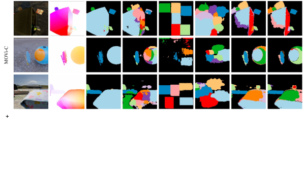
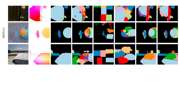
Figure 7: Additional examples of failure cases on MOVi-A and MOVi-C. ^†– indicates post-processing.

Qualitative results on MOVi-A and MOVi-C.

In  Fig. 5 and  6 we show additional qualitative results on MOVi-A and MOVi-C respectively. Following the results in main paper, the segments discovered by our method are semantically meaningful. Our object boundaries are of higher quality than the comparable methods. GWM suffers from oversegmentation of the objects. SCALOR has dificulty with complex datasets, such as MOVi-C as observed in Fig. 6. SAVI’s object boundaries do not conform to object shape. We also provide additional failure cases of our model in Fig. 7. Our model has difficulty with objects that have complex motion for our affine formulation to model ably.

References

• Adiv [1985] Gilad Adiv. Determining three-dimensional motion and structure from optical flow generated by several moving objects. IEEE transactions on pattern analysis and machine intelligence, (4):384–401, 1985.
• Arbelaez et al. [2014] Pablo Arbelaez, Jordi Pont-Tuset, Jonathan T. Barron, Ferran Marques, and Jitendra Malik. Multiscale combinatorial grouping. In Proceedings of the IEEE Conference on Computer Vision and Pattern Recognition (CVPR), June 2014.
• Bao et al. [2022] Zhipeng Bao, Pavel Tokmakov, Allan Jabri, Yu-Xiong Wang, Adrien Gaidon, and Martial Hebert. Discovering objects that can move. In Proceedings of the IEEE/CVF Conference on Computer Vision and Pattern Recognition (CVPR), pages 11789–11798, June 2022.
• Bergen et al. [1992] James R Bergen, Patrick Anandan, Keith J Hanna, and Rajesh Hingorani. Hierarchical model-based motion estimation. In European conference on computer vision, pages 237–252. Springer, 1992.
• Burgess et al. [2019] Christopher P Burgess, Loic Matthey, Nicholas Watters, Rishabh Kabra, Irina Higgins, Matt Botvinick, and Alexander Lerchner. Monet: Unsupervised scene decomposition and representation. arXiv preprint arXiv:1901.11390, 2019.
• Cheng et al. [2022] Bowen Cheng, Ishan Misra, Alexander G Schwing, Alexander Kirillov, and Rohit Girdhar. Masked-attention mask transformer for universal image segmentation. In Proceedings of the IEEE/CVF Conference on Computer Vision and Pattern Recognition, pages 1290–1299, 2022.
• Choudhury et al. [2021] Subhabrata Choudhury, Iro Laina, Christian Rupprecht, and Andrea Vedaldi. Unsupervised part discovery from contrastive reconstruction. In Advances in Neural Information Processing Systems, volume 35, 2021.
• Choudhury et al. [2022] Subhabrata Choudhury, Laurynas Karazija, Iro Laina, Andrea Vedaldi, and Christian Rupprecht. Guess What Moves: Unsupervised video and image segmentation by anticipating motion. In British Machine Vision Conference (BMVC), 2022.
• Crawford and Pineau [2019] Eric Crawford and Joelle Pineau. Spatially invariant unsupervised object detection with convolutional neural networks. In Proceedings of the AAAI Conference on Artificial Intelligence, volume 33, pages 3412–3420, 2019.
• Dutt Jain et al. [2017] Suyog Dutt Jain, Bo Xiong, and Kristen Grauman. Fusionseg: Learning to combine motion and appearance for fully automatic segmentation of generic objects in videos. In Proceedings of the IEEE conference on computer vision and pattern recognition, pages 3664–3673, 2017.
• Emami et al. [2021] Patrick Emami, Pan He, Sanjay Ranka, and Anand Rangarajan. Efficient iterative amortized inference for learning symmetric and disentangled multi-object representations. In Proceedings of the 38th International Conference on Machine Learning, pages 2970–2981. PMLR, 2021.
• Engelcke et al. [2020] Martin Engelcke, Adam R Kosiorek, Oiwi Parker Jones, and Ingmar Posner. Genesis: Generative scene inference and sampling with object-centric latent representations. In International Conference on Learning Representations, 2020.
• Engelcke et al. [2021] Martin Engelcke, Oiwi Parker Jones, and Ingmar Posner. Genesis-v2: Inferring unordered object representations without iterative refinement. In Advances in Neural Information Processing Systems, volume 34, 2021.
• Eslami et al. [2016] S. M. Ali Eslami, Nicolas Heess, Theophane Weber, Yuval Tassa, David Szepesvari, Koray Kavukcuoglu, and Geoffrey E. Hinton. Attend, infer, repeat: Fast scene understanding with generative models. In Proceedings of the 30th International Conference on Neural Information Processing Systems, page 3233–3241, 2016.
• Faktor and Irani [2014] Alon Faktor and Michal Irani. Video segmentation by non-local consensus voting. In Proceedings of the British Machine Vision Conference. BMVA Press, 2014.
• Geiger et al. [2012] Andreas Geiger, Philip Lenz, and Raquel Urtasun. Are we ready for autonomous driving? The KITTI vision benchmark suite. In Proceedings of the IEEE/CVF Conference on Computer Vision and Pattern Recognition (CVPR), pages 3354–3361. IEEE, 2012.
• Greff et al. [2015] Klaus Greff, Rupesh Kumar Srivastava, and Jürgen Schmidhuber. Binding via reconstruction clustering. ArXiv, abs/1511.06418, 2015.
• Greff et al. [2016] Klaus Greff, Antti Rasmus, Mathias Berglund, Tele Hao, Harri Valpola, and Jürgen Schmidhuber. Tagger: Deep unsupervised perceptual grouping. In Advances in Neural Information Processing Systems, pages 4484–4492, 2016.
• Greff et al. [2019] Klaus Greff, Raphaël Lopez Kaufman, Rishabh Kabra, Nick Watters, Christopher Burgess, Daniel Zoran, Loic Matthey, Matthew Botvinick, and Alexander Lerchner. Multi-object representation learning with iterative variational inference. In International Conference on Machine Learning, pages 2424–2433. PMLR, 2019.
• Greff et al. [2022] Klaus Greff, Francois Belletti, Lucas Beyer, Carl Doersch, Yilun Du, Daniel Duckworth, David J Fleet, Dan Gnanapragasam, Florian Golemo, Charles Herrmann, Thomas Kipf, Abhijit Kundu, Dmitry Lagun, Issam Laradji, Hsueh-Ti (Derek) Liu, Henning Meyer, Yishu Miao, Derek Nowrouzezahrai, Cengiz Oztireli, Etienne Pot, Noha Radwan, Daniel Rebain, Sara Sabour, Mehdi S. M. Sajjadi, Matan Sela, Vincent Sitzmann, Austin Stone, Deqing Sun, Suhani Vora, Ziyu Wang, Tianhao Wu, Kwang Moo Yi, Fangcheng Zhong, and Andrea Tagliasacchi. Kubric: a scalable dataset generator. In Proceedings of the IEEE Conference on Computer Vision and Pattern Recognition (CVPR), 2022.
• He et al. [2019] Zhen He, Jian Li, Daxue Liu, Hangen He, and David Barber. Tracking by animation: Unsupervised learning of multi-object attentive trackers. 2019 IEEE/CVF Conference on Computer Vision and Pattern Recognition (CVPR), pages 1318–1327, 2019.
• Jang et al. [2017] Eric Jang, Shixiang Gu, and Ben Poole. Categorical reparameterization with gumbel-softmax. In 5th International Conference on Learning Representations, ICLR, 2017.
• Jiang and Ahn [2020] Jindong Jiang and Sungjin Ahn. Generative neurosymbolic machines. In Advances in Neural Information Processing Systems, volume 33, pages 12572–12582, 2020.
• Jiang et al. [2020] Jindong Jiang, Sepehr Janghorbani, Gerard De Melo, and Sungjin Ahn. Scalor: Generative world models with scalable object representations. In International Conference on Learning Representations, 2020.
• Johnson et al. [2017] Justin Johnson, Bharath Hariharan, Laurens Van Der Maaten, Li Fei-Fei, C Lawrence Zitnick, and Ross Girshick. CLEVR: A diagnostic dataset for compositional language and elementary visual reasoning. In Proceedings of the IEEE Conference on Computer Vision and Pattern Recognition, pages 2901–2910, 2017.
• Kabra et al. [2021] Rishabh Kabra, Daniel Zoran, Goker Erdogan, Loïc Matthey, Antonia Creswell, Matthew M. Botvinick, Alexander Lerchner, and Christopher P. Burgess. SIMONe: View-invariant, temporally-abstracted object representations via unsupervised video decomposition. volume 34, pages 20146–20159, 2021.
• Karazija et al. [2021] Laurynas Karazija, Iro Laina, and Christian Rupprecht. Clevrtex: A texture-rich benchmark for unsupervised multi-object segmentation. In Thirty-fifth Conference on Neural Information Processing Systems Datasets and Benchmarks Track, 2021.
• Kipf et al. [2022] Thomas Kipf, Gamaleldin Fathy Elsayed, Aravindh Mahendran, Austin Stone, Sara Sabour, Georg Heigold, Rico Jonschkowski, Alexey Dosovitskiy, and Klaus Greff. Conditional object-centric learning from video. In International Conference on Learning Representations, 2022.
• Kosiorek et al. [2018] Adam Kosiorek, Hyunjik Kim, Yee Whye Teh, and Ingmar Posner. Sequential attend, infer, repeat: Generative modelling of moving objects. Advances in Neural Information Processing Systems, 31, 2018.
• Kossen et al. [2020] Jannik Kossen, Karl Stelzner, Marcel Hussing, Claas Voelcker, and Kristian Kersting. Structured object-aware physics prediction for video modeling and planning. In Proceedings of the International Conference on Learning Representations, 2020.
• Li et al. [2020] Nanbo Li, Cian Eastwood, and Robert Fisher. Learning object-centric representations of multi-object scenes from multiple views. Advances in Neural Information Processing Systems, 33:5656–5666, 2020.
• Li et al. [2018] Siyang Li, Bryan Seybold, Alexey Vorobyov, Alireza Fathi, Qin Huang, and C-C Jay Kuo. Instance embedding transfer to unsupervised video object segmentation. In Proceedings of the IEEE conference on computer vision and pattern recognition, pages 6526–6535, 2018.
• Lin et al. [2020a] Zhixuan Lin, Yi-Fu Wu, Skand Peri, Bofeng Fu, Jindong Jiang, and Sungjin Ahn. Improving generative imagination in object-centric world models. In International Conference on Machine Learning, pages 6140–6149. PMLR, 2020a.
• Lin et al. [2020b] Zhixuan Lin, Yi-Fu Wu, Skand Vishwanath Peri, Weihao Sun, Gautam Singh, Fei Deng, Jindong Jiang, and Sungjin Ahn. SPACE: Unsupervised object-oriented scene representation via spatial attention and decomposition. In International Conference on Learning Representations, 2020b.
• Liu et al. [2020] Liang Liu, Jiangning Zhang, Ruifei He, Yong Liu, Yabiao Wang, Ying Tai, Donghao Luo, Chengjie Wang, Jilin Li, and Feiyue Huang. Learning by analogy: Reliable supervision from transformations for unsupervised optical flow estimation. In Proceedings of the IEEE/CVF Conference on Computer Vision and Pattern Recognition (CVPR), June 2020.
• Liu et al. [2021] Ze Liu, Yutong Lin, Yue Cao, Han Hu, Yixuan Wei, Zheng Zhang, Stephen Lin, and Baining Guo. Swin transformer: Hierarchical vision transformer using shifted windows. In Proceedings of the IEEE/CVF International Conference on Computer Vision, pages 10012–10022, 2021.
• Locatello et al. [2020] Francesco Locatello, Dirk Weissenborn, Thomas Unterthiner, Aravindh Mahendran, Georg Heigold, Jakob Uszkoreit, Alexey Dosovitskiy, and Thomas Kipf. Object-centric learning with slot attention. In Advances in Neural Information Processing Systems, volume 33, pages 11525–11538, 2020.
• Loshchilov and Hutter [2017] Ilya Loshchilov and Frank Hutter. Decoupled weight decay regularization. arXiv preprint arXiv:1711.05101, 2017.
• Lu et al. [2019] Xiankai Lu, Wenguan Wang, Chao Ma, Jianbing Shen, Ling Shao, and Fatih Porikli. See more, know more: Unsupervised video object segmentation with co-attention siamese networks. In Proceedings of the IEEE/CVF Conference on Computer Vision and Pattern Recognition, pages 3623–3632, 2019.
• Maddison et al. [2017] Chris J Maddison, Andriy Mnih, and Yee Whye Teh. The concrete distribution: A continuous relaxation of discrete random variables. In 5th International Conference on Learning Representations, ICLR, 2017.
• Mahendran et al. [2018] Aravindh Mahendran, James Thewlis, and Andrea Vedaldi. Self-supervised segmentation by grouping optical-flow. In Proceedings of the European Conference on Computer Vision (ECCV) Workshops, September 2018.
• Meunier et al. [2022] Etienne Meunier, Anaïs Badoual, and Patrick Bouthemy. EM-driven unsupervised learning for efficient motion segmentation. arXiv preprint arXiv:2201.02074, 2022.
• Monnier et al. [2021] Tom Monnier, Elliot Vincent, Jean Ponce, and Mathieu Aubry. Unsupervised layered image decomposition into object prototypes. In Proceedings of the IEEE/CVF International Conference on Computer Vision (ICCV), pages 8640–8650, 2021.
• Papazoglou and Ferrari [2013] Anestis Papazoglou and Vittorio Ferrari. Fast object segmentation in unconstrained video. In Proceedings of the IEEE International Conference on Computer Vision (ICCV), December 2013.
• Ronneberger et al. [2015] Olaf Ronneberger, Philipp Fischer, and Thomas Brox. U-net: Convolutional networks for biomedical image segmentation. In International Conference on Medical image computing and computer-assisted intervention, pages 234–241. Springer, 2015.
• Singh et al. [2021] Gautam Singh, Skand Peri, Junghyun Kim, Hyunseok Kim, and Sungjin Ahn. Structured world belief for reinforcement learning in POMDP. In International Conference on Machine Learning, pages 9744–9755. PMLR, 2021.
• Smirnov et al. [2021] Dmitriy Smirnov, Michael Gharbi, Matthew Fisher, Vitor Guizilini, Alexei A Efros, and Justin Solomon. Marionette: Self-supervised sprite learning. In Advances in Neural Information Processing Systems, volume 34, 2021.
• Stelzner et al. [2019] Karl Stelzner, Robert Peharz, and Kristian Kersting. Faster attend-infer-repeat with tractable probabilistic models. In Proceedings of the 36th International Conference on Machine Learning, volume 97, pages 5966–5975. PMLR, 2019.
• Stone et al. [2021] Austin Stone, Daniel Maurer, Alper Ayvaci, Anelia Angelova, and Rico Jonschkowski. Smurf: Self-teaching multi-frame unsupervised raft with full-image warping. 2021 IEEE/CVF Conference on Computer Vision and Pattern Recognition (CVPR), pages 3886–3895, 2021.
• Teed and Deng [2020] Zachary Teed and Jia Deng. Raft: Recurrent all-pairs field transforms for optical flow. In European Conference on Computer Vision (ECCV), 2020.
• Tokmakov et al. [2019] Pavel Tokmakov, Cordelia Schmid, and Karteek Alahari. Learning to segment moving objects. International Journal of Computer Vision, 127(3):282–301, mar 2019.
• Torr [1998] Philip H. S. Torr. Geometric motion segmentation and model selection. Philosophical Transactions of the Royal Society of London. Series A: Mathematical, Physical and Engineering Sciences, 356:1321 – 1340, 1998.
• Tsai et al. [2016] Yi-Hsuan Tsai, Ming-Hsuan Yang, and Michael J. Black. Video segmentation via object flow. In 2016 IEEE Conference on Computer Vision and Pattern Recognition (CVPR), pages 3899–3908, 2016.
• Van Steenkiste et al. [2018] Sjoerd Van Steenkiste, Michael Chang, Klaus Greff, and Jürgen Schmidhuber. Relational neural expectation maximization: Unsupervised discovery of objects and their interactions. arXiv preprint arXiv:1802.10353, 2018.
• Veerapaneni et al. [2020] Rishi Veerapaneni, John D Co-Reyes, Michael Chang, Michael Janner, Chelsea Finn, Jiajun Wu, Joshua Tenenbaum, and Sergey Levine. Entity abstraction in visual model-based reinforcement learning. In Conference on Robot Learning, pages 1439–1456. PMLR, 2020.
• Weis et al. [2021] Marissa A. Weis, Kashyap Chitta, Yash Sharma, Wieland Brendel, Matthias Bethge, Andreas Geiger, and Alexander S. Ecker. Benchmarking unsupervised object representations for video sequences. Journal of Machine Learning Research, 22(183):1–61, 2021.
• Wu et al. [2021] Yizhe Wu, Oiwi Parker Jones, Martin Engelcke, and Ingmar Posner. Apex: Unsupervised, object-centric scene segmentation and tracking for robot manipulation. 2021 IEEE/RSJ International Conference on Intelligent Robots and Systems (IROS), pages 3375–3382, 2021.
• Xu et al. [2019] Kun Xu, Chongxuan Li, Jun Zhu, and Bo Zhang. Multi-object generation with amortized structural regularization. In Proceedings of the 33rd International Conference on Neural Information Processing Systems. Curran Associates Inc., 2019.
• Yang et al. [2021] Charig Yang, Hala Lamdouar, Erika Lu, Andrew Zisserman, and Weidi Xie. Self-supervised video object segmentation by motion grouping. In Proceedings of the IEEE/CVF International Conference on Computer Vision, pages 7177–7188, 2021.
• Yang et al. [2019] Yanchao Yang, Antonio Loquercio, Davide Scaramuzza, and Stefano Soatto. Unsupervised moving object detection via contextual information separation. In Proceedings of the IEEE/CVF Conference on Computer Vision and Pattern Recognition (CVPR), June 2019.
• Zablotskaia et al. [2021] Polina Zablotskaia, Edoardo A. Dominici, Leonid Sigal, and Andreas M. Lehrmann. Provide: a probabilistic framework for unsupervised video decomposition. In Proceedings of the Thirty-Seventh Conference on Uncertainty in Artificial Intelligence, volume 161, pages 2019–2028. PMLR, 2021.