Geometric Sparse Coding in Wasserstein Space

Abstract

Wasserstein dictionary learning is an unsupervised approach to learning a collection of probability distributions that generate observed distributions as Wasserstein barycentric combinations. Existing methods for Wasserstein dictionary learning optimize an objective that seeks a dictionary with sufficient representation capacity via barycentric interpolation to approximate the observed training data, but without imposing additional structural properties on the coefficients associated to the dictionary. This leads to dictionaries that densely represent the observed data, which makes interpretation of the coefficients challenging and may also lead to poor empirical performance when using the learned coefficients in downstream tasks. In contrast and motivated by sparse dictionary learning in Euclidean spaces, we propose a geometrically sparse regularizer for Wasserstein space that promotes representations of a data point using only nearby dictionary elements. We show this approach leads to sparse representations in Wasserstein space and addresses the problem of non-uniqueness of barycentric representation. Moreover, when data is generated as Wasserstein barycenters of fixed distributions, this regularizer facilitates the recovery of the generating distributions in cases that are ill-posed for unregularized Wasserstein dictionary learning. Through experimentation on synthetic and real data, we show that our geometrically regularized approach yields sparser and more interpretable dictionaries in Wasserstein space, which perform better in downstream applications.

1 Introduction

A central goal of statistical signal processing is the discovery of latent structures in complex data. Indeed, although data often resides in a high-dimensional ambient space, the classical manifold hypothesis posits that in fact, the data can be well approximated by low-dimensional manifolds or mixtures thereof, which circumvents the curse of dimensionality that plagues high-dimensional statistics. Linear dimensionality reduction methods such as principal component analysis (PCA) (Hotelling,, 1933) and non-linear manifold learning approaches that exploit local connectivity structure in the data (Scholkopf et al.,, 1997; Tenenbaum et al.,, 2000; Roweis and Saul,, 2000; Belkin and Niyogi,, 2003; Coifman and Lafon,, 2006) rely on this assumption of intrinsically low-dimensional structure in high-dimensional data to glean insights. These techniques typically output a low-dimensional representation preserving local geometric structures such as pairwise distances or geodesic distances with respect to a Riemannian metric.

An alternative perspective for efficiently representing complex data is the sparse coding and dictionary learning paradigm (Olshausen and Field,, 1996, 1997; Barlow et al.,, 1961; Hromádka et al.,, 2008). In the simplest setting when data is considered as elements of $\mathbb{R}^{d}$ (or more generally a normed vector space), the aim of sparse coding is to represent data $\{\mathbf{y}_{i}\}_{i=1}^{n}\subset\mathbb{R}^{d}$, stacked as rows in the matrix $\mathbf{Y}\in\mathbb{R}^{n\times d}$, as a linear combination of vectors $\{\mathbf{d}_{j}\}_{j=1}^{m}$, stacked as a dictionary matrix $\mathbf{D}\in\mathbb{R}^{m\times d}$ such that $\mathbf{Y}\approx\mathbf{\Lambda}\mathbf{D}$ for some coefficients $\mathbf{\Lambda}\in\mathbb{R}^{n\times m}$, perhaps subject to constraints on $\mathbf{\Lambda}$. When the dictionary $\mathbf{D}$ is fixed, this reduces to an optimization over $\mathbf{\Lambda}$ (Mallat,, 1999; Engan et al.,, 2000). More generally, $\mathbf{D}$ and $\mathbf{\Lambda}$ can be learned simultaneously with some additional constraints on the dictionary or coefficients (Lee and Seung,, 1999; Aharon et al.,, 2006). This is typically formulated as an optimization problem

$$\operatorname*{arg\,min}_{\mathbf{D},\mathbf{\Lambda}}\,\,\mathcal{L}(\mathbf{Y},\mathbf{\Lambda}\mathbf{D})+\rho\,\mathcal{R}(\mathbf{D},\mathbf{\Lambda}),$$ (1)

for some loss function $\mathcal{L}$ (e.g., $\mathcal{L}(\mathbf{Y},\mathbf{\Lambda}\mathbf{D})=\|\mathbf{Y}-\mathbf{\Lambda}\mathbf{D}\|_{F}$) and regularization function $\mathcal{R}$ (e.g., $\mathcal{R}(\mathbf{D},\mathbf{\Lambda})=\|\mathbf{\Lambda}\|_{1}$) balanced by a parameter $\rho>0$. The regularizers ensure well-posedness of the problem and improve interpretability and robustness. The problem (1) is the dictionary learning problem in $\mathbb{R}^{d}$.

The imposed Euclidean structure is convenient computationally but limiting in practice, as many real data are better modeled as living in spaces with non-Euclidean geometry where instead $\mathbf{Y}\approx\mathcal{F}(\mathbf{D},\mathbf{\Lambda})$ for some nonlinear reconstruction function $\mathcal{F}$ (Tuzel et al.,, 2006, 2007; Li et al.,, 2008; Guo et al.,, 2010; Harandi et al.,, 2013, 2015; Cherian and Sra,, 2016; Yin et al.,, 2016; Maggioni et al.,, 2016; Liu et al.,, 2018; Schmitz et al.,, 2018; Tankala et al.,, 2020). Important questions in this setting are what notion of reconstruction should take the place of linear combination (i.e. $\mathcal{F}$), how reconstruction quality is assessed without the use of a global norm (i.e. $\mathcal{L}$), and what constraints are natural on the coefficients in the nonlinear space (i.e. $\mathcal{R}$).

This paper focuses on nonlinear sparse coding and dictionary learning for data that are modeled as probability distributions in Wasserstein space. This basic framework was pioneered by Schmitz et al., (2018), where the authors leverage the theory and algorithms of optimal transport to propose the Wasserstein dictionary learning (WDL) algorithm, whereby a data point (interpreted as a probability distribution or histogram in $\mathbb{R}^{d}$) is approximated as a Wasserstein barycenter (Agueh and Carlier,, 2011) of the learned dictionary atoms. The resulting framework is focused on learning a dictionary that reconstructs well, but neglects other desirable aspects of a dictionary such as sparsity of the induced coefficients. Moreover, this classical scheme is ill-posed in two senses: for a fixed dictionary, unique coefficients are not assured; moreover, there may be multiple dictionaries that enable perfect reconstruction of the observed data.

Summary of Contributions: We generalize the classical WDL algorithm (Schmitz et al.,, 2018) by incorporating a novel Wasserstein geometric sparse regularizer. Our regularizer encourages an observed data point to be reconstructed as a barycentric representation from nearby (in the sense of Wasserstein distances) dictionary atoms. As we vary the balance parameter for this regularizer, the proposed method interpolates between classical WDL (no regularization) and Wasserstein $K$-means (strong regularization). Unlike the original formulation, the proposed regularizer learns dictionary atoms with geometric similarity to the training data. Theoretically, we demonstrate the ability of the model to learn sparse coefficients and to overcome issues of non-uniqueness both at the level of learning coefficients for a fixed dictionary, and for the general WDL problem on an idealized generative model in Wasserstein space. Empirically, we provide evidence that our regularized dictionary learning scheme yields more interpretable and useful coefficients for downstream classification tasks; the code to reproduce all experiments in this paper will be released on the authors’ GitHub.

Notations and Preliminaries: Lowercase and uppercase boldface letters denote (column) vectors and matrices, respectively. We generally use Greek letters to denote measures, with the exception that $\mathcal{D}=\{\mathcal{D}\}_{j=1}^{m}$ denotes the dictionary when its elements are measures. We denote the Euclidean norm of a vector $\mathbf{x}$ as $||\mathbf{x}||_{2}$. Let

$$\Delta^{m}=\left\{\mathbf{x}\in\mathbb{R}^{m}\ \bigg{|}\ \sum_{i=1}^{m}x_{i}=1,\forall i=1,\ldots,m,x_{i}\geq 0\right\}$$

denote the discrete probability simplex of dimension $m$. Softmax, as a change of variables, is defined as $\operatorname{CoV}(\mathbf{x}):=\exp(\mathbf{x})/\exp(\mathbf{x})^{T}\mathbbm{1}_{N}$. Here we take the exponential to be an elementwise operation on the vector and use $\mathbbm{1}_{N}$ to denote the ones vector of size $N$. When we write $\operatorname{CoV}(\mathbf{X})$ for some matrix $\mathbf{X}\in\mathbb{R}^{n\times m}$ we take it to mean applying the change of variables to each row.

2 Background and Related Work

Classical Dictionary Learning: In equation (1), using $\mathcal{L}(\mathbf{Y},\mathbf{\Lambda}\mathbf{D})=\|\mathbf{Y}-\mathbf{\Lambda}\mathbf{D}\|_{F}$ and $\rho=0$ yields an optimization problem with optimal dictionary and coefficients given by the $m$ singular components with largest singular values (Eckart and Young,, 1936). To promote interpretable, sparse coefficients that still realize $\mathbf{Y}\approx\mathbf{\Lambda}\mathbf{D}$, the prototypical regularized dictionary learning problem is $\underset{\mathbf{D},\mathbf{\Lambda}}{\min}\,||\mathbf{Y}-\mathbf{\Lambda}\mathbf{D}||_{F}^{2}+\rho||\mathbf{\Lambda}||_{1}$ where $||\mathbf{\Lambda}||_{1}=\sum_{i=1}^{n}\sum_{j=1}^{m}|\Lambda_{ij}|$ is a sparsity-promoting regularizer (Donoho,, 2006; Elad,, 2010). Beyond enhancing interpretability, efficiency, and uniqueness of representation, sparse representations improve generalization of efficient supervised learning (Mehta and Gray,, 2013; Mairal et al.,, 2011). In the non-negative matrix factorization (NMF) paradigm, non-negativity constraints are imposed on the atoms and coefficients, which increases their interpretability and effectiveness in downstream applications (Lee and Seung,, 1999, 2000; Berry et al.,, 2007).

Optimal Transport: We provide basic background on optimal transport; for more general treatments and theory, see (Ambrosio et al.,, 2005; Villani,, 2021; Santambrogio,, 2015; Peyré et al.,, 2019). Let $\mathcal{P}(\mathbb{R}^{d})$ be the space of probability measures in $\mathbb{R}^{d}$. Let $\mu,\nu\in\mathcal{P}(\mathbb{R}^{d})$. Let

$$\Pi(\mu,\nu)= \{\gamma:\mathbb{R}^{d}\times\mathbb{R}^{d}\rightarrow\mathbb{R}\ |\ \text{for all }A,B\text{ Borel},\ \gamma(A\times\mathbb{R}^{d})=\mu(A),\ \gamma(\mathbb{R}^{d}\times B)=\nu(B)\}$$

be the set of joint distributions with marginals $\mu$ and $\nu$. The squared Wasserstein$-2$ distance is defined as:

$$W_{2}^{2}(\mu,\nu):=\min_{\pi\in\Pi(\mu,\nu)}\int_{\mathbb{R}^{d}\times\mathbb{R}^{d}}\|\mathbf{x}-\mathbf{y}\|_{2}^{2}\ \pi(\mathbf{x},\mathbf{y}).$$ (2)

Given measures $\{\mathcal{D}_{j}\}_{j=1}^{m}\subset\mathcal{P}(\mathbb{R}^{d})$ that have finite second moments, along with a vector $\boldsymbol{\lambda}\in\Delta^{m}$, the Wasserstein-(2) barycenter (Agueh and Carlier,, 2011) is defined as:

$$\operatorname{Bary}(\mathcal{D},\boldsymbol{\lambda}):=\operatorname*{arg\,min}_{\mu\in\mathcal{P}(\mathbb{R}^{d})}\sum_{j=1}^{m}\lambda_{j}W_{2}^{2}(\mathcal{D}_{j},\mu).$$ (3)

The measure $\operatorname{Bary}(\mathcal{D},\boldsymbol{\lambda})$ can be interpreted as a weighted average of the $\{\mathcal{D}_{j}\}_{j=1}^{m}$, with the impact of $\mathcal{D}_{j}$ proportional to $\lambda_{j}$. Wasserstein barycenters have proven useful in a range of applications, and are in a precise sense the “correct” way to combine measures, in that $\operatorname{Bary}(\mathcal{D},\boldsymbol{\lambda})$ preserves the geometric properties of $\mathcal{D}=\{\mathcal{D}_{j}\}_{j=1}^{m}$ in a way that linear mixtures do not (Agueh and Carlier,, 2011; Rabin et al.,, 2011; Cuturi and Doucet,, 2014; Bonneel et al.,, 2016). Wasserstein barycenters are intimately connected to geodesics in Wasserstein space, in the following sense. For $\pi^{*}$ optimizing (2), the McCann interpolation of $\mu,\nu$ is $(P_{t})_{\#}\pi^{*}$ where $P_{t}(\mathbf{x},\mathbf{y})=(1-t)\mathbf{x}+t\mathbf{y}$ for $t\in[0,1]$ and where $(P_{t})_{\#}$ denotes the pushforward by $P_{t}$. The McCann interpolation is the constant-speed geodesic between $\mu,\nu$ in the Wasserstein-2 space (McCann,, 1997; Ambrosio et al.,, 2005) and coincides with the Wasserstein barycenter with weight $\boldsymbol{\lambda}=(1-t,t)$ on $\mu,\nu$.

3 Geometric Sparse Regularization for Wasserstein Dictionary Learning

WDL (Schmitz et al.,, 2018) aims to find a dictionary of probability distributions $\mathcal{D}=\{\mathcal{D}_{j}\}_{j=1}^{m}\subset\mathcal{P}(\mathbb{R}^{d})$ such that observed data $\{\mu_{i}\}_{i=1}^{n}\subset\mathcal{P}(\mathbb{R}^{d})$ can be represented as Wasserstein barycenters of the collection $\mathcal{D}$. The precise optimization problem is

$$\operatorname*{arg\,min}_{\begin{subarray}{c}\mathcal{D}\in\mathcal{P}(\mathbb{R}^{d})^{m}\\ \mathbf{\Lambda}\in(\Delta^{m})^{n}\end{subarray}}\,\,\sum_{i=1}^{n}\mathcal{L}(\operatorname{Bary}(\mathcal{D},\boldsymbol{\lambda}_{i}),\mu_{i}),$$ (4)

where the loss function $\mathcal{L}$ is typically taken to be $W_{2}^{2}$ and $\boldsymbol{\lambda}_{i}\in\Delta^{m}$ is a (column) vector of size $m$, corresponding to a row of $\mathbf{\Lambda}$. In other words, solving this problem finds the dictionary of probability distributions that finds best approximations to each data point $\mu_{i}$ using barycentric combinations of $\mathcal{D}$. WDL was proposed in part as an alternative to geodesic principal component analysis in Wasserstein space (Boissard et al.,, 2015; Seguy and Cuturi,, 2015; Bigot et al.,, 2017), and has proven highly effective in terms of producing meaningful atoms for representing probability distributions. However, it may yield non-sparse coefficients. Moreover, as we will establish, it is ill-posed both at the level of having non-unique coefficients for a fixed dictionary $\mathcal{D}$ and at the level of having multiple dictionaries that can reconstruct the data perfectly.

Thus, one might consider adding the $\ell_{1}$ regularizer to the WDL objective to induce desirable sparsity of the representation. However, this fails because all coefficients of a Wasserstein barycenter lie on $\Delta^{m}$. Methods to promote sparsity of coefficients on the simplex can be done with entropy, projections, and suitable use of the the $\ell^{2}$ norm (Donoho et al.,, 1992; Shashanka et al.,, 2007; Larsson and Ugander,, 2011; Kyrillidis et al.,, 2013; Li et al.,, 2020), but we focus instead on geometric regularization. An analogous problem has been studied in the linear setting in a situation where the weights are on $\Delta^{m}$ (Tankala et al.,, 2020). In that context, the geometric sparse regularizer $\displaystyle\sum_{j=1}^{m}\lambda_{j}||\mathbf{y}-\mathbf{d}_{j}||_{2}^{2}$ (for an individual data point $\mathbf{y}$ with representation coefficient $\boldsymbol{\lambda}$) has been proven to promote sparsity by favoring local representations, namely reconstructing using nearby (with respect to Euclidean distances) dictionary atoms.

We propose to regularize (4) with a novel Wasserstein geometric sparse regularizer:

$$\mathcal{R}(\mathcal{D},\mathbf{\Lambda}):=\sum_{i=1}^{n}\sum_{j=1}^{m}(\boldsymbol{\lambda}_{i})_{j}W_{2}^{2}(\mathcal{D}_{j},\mu_{i}).$$ (5)

This yields a new, regularized objective:

$$\mathcal{F}(\mathcal{D},\mathbf{\Lambda},\{\mu_{i}\}_{i=1}^{n}):= \min_{\begin{subarray}{c}\mathcal{D}\in\mathcal{P}(\mathbb{R}^{d})^{m}\\ \mathbf{\Lambda}\in(\Delta^{m})^{n}\end{subarray}}\,\,\sum_{i=1}^{n}W_{2}^{2}(\operatorname{Bary}(\mathcal{D},\boldsymbol{\lambda}_{i}),\mu_{i})+\rho\sum_{i=1}^{n}\sum_{j=1}^{m}(\boldsymbol{\lambda}_{i})_{j}W_{2}^{2}(\mathcal{D}_{j},\mu_{i}),$$ (6)

where $\rho>0$ is a tuneable balance parameter.

Note that the geometric sparse regularizer (5) resembles the objective in the definition of the Wasserstein barycenter in (3). Crucially, in the unregularized formulation of the WDL problem, the distance from the atoms to the data points is only indirectly minimized, because the WDL formulation focuses solely on the reconstruction accuracy of the generated barycenters and not directly about how similar those atoms are to the data points. As such, the atoms may be arbitrarily far from the data provided that the reconstruction accuracy is low. As discussed below, this may cause the existence of arbitrarily many solutions to the WDL problem (4), which in general is ill-posed.

Interpretations of $\mathcal{R}(\mathcal{D},\mathbf{\Lambda})$: The regularization term $\mathcal{R}(\mathcal{D},\mathbf{\Lambda})$ is analogous to Laplacian smoothing in Euclidean space (Cai et al.,, 2010; Dornaika and Weng,, 2019) and can be interpreted as non-linear archetypal learning (Cutler and Breiman,, 1994) in Wasserstein space. As previously mentioned, there is no notion of sparse coding in the unregularized WDL formulation. The geometric sparse regularizer promotes sparsity by penalizing the use of atoms that are far from the data to be represented and thus acts as a weighted $\ell_{1}$ norm on the coefficients (Tasissa et al.,, 2021).

Connection with Wasserstein $K$-means: In this problem (Domazakis et al.,, 2019; Verdinelli and Wasserman,, 2019; Zhuang et al.,, 2022), given observed measures $\{\mu_{i}\}_{i=1}^{n}\subset\mathcal{P}(\mathbb{R}^{d})$ we want to find “centers” $\mathcal{D}=\{\mathcal{D}_{j}\}_{j=1}^{m}\subset\mathcal{P}(\mathbb{R}^{d})$ solving the optimization problem

$$\underset{\mathbf{C},\mathcal{D}}{\min}\,\,\sum_{i=1}^{n}\sum_{j=1}^{m}C_{ij}W_{2}^{2}(\mathcal{D}_{j},\mu_{i}),$$

where $\mathbf{C}\in\mathbb{R}^{n\times m}$ is such that $C_{ij}\in\{0,1\}$ is a binary assignment variable satisfying $\sum_{j=1}^{m}C_{ij}=1$ for all $i=1,\dots,n$. Suppose $\mathcal{D}^{*}\in\mathcal{P}(\mathbb{R}^{d})^{m}$ and $\mathbf{\Lambda}^{*}\in\mathbb{R}^{n\times m}$ are the optimizers of (6). Note that for any feasible $\mathbf{\Lambda}$ and with dictionary fixed at $\mathcal{D}^{*}$, we have

$$\mathcal{R}(\mathcal{D}^{*},\mathbf{\Lambda})= \sum_{i=1}^{n}\sum_{j=1}^{m}(\boldsymbol{\lambda}_{i})_{j}W_{2}^{2}(\mathcal{D}^{*}_{j},\mu_{i})$$

$$\geq \sum_{i=1}^{n}\sum_{j=1}^{m}(\boldsymbol{\lambda}_{i})_{j}\underset{1\leq p\leq m}{\min}W_{2}^{2}(\mathcal{D}^{*}_{p},\mu_{i})$$

$$= \sum_{i=1}^{n}\underset{1\leq p\leq m}{\min}W_{2}^{2}(\mathcal{D}^{*}_{p},\mu_{i}).$$

Thus, for fixed $\mathcal{D}^{*}$, coefficients that minimize $\mathcal{R}(\mathcal{D}^{*},\mathbf{\Lambda})$ have the property that the $i^{th}$ row is all zeros except for a $1$ at the $i^{*}$ position where $i^{*}=\underset{1\leq p\leq m}{\operatorname*{arg\,min}}\,\,W_{2}^{2}(\mathcal{D}^{*}_{p},\mu_{i})$. In this sense, for a fixed dictionary $\mathcal{D}^{*}$ and with each observation $\mu_{1},\dots,\mu_{n}$ having a unique nearest neighbor in $\mathcal{D}^{*}$, the optimal solution $\mathbf{\Lambda}^{*}$ is a matrix whose rows are binary and $1$-sparse, which is exactly of the same form as the binary assignment in Wasserstein $K$-means. When the aforementioned assumption does not hold, uniqueness is not guaranteed but the $1$-sparse solution is in the family of optimal solutions.

In this sense, incorporating the geometric sparse regularizer (5) into the main objective in (4) with a scaling parameter $\rho$ enables interpolation between learning a dictionary for pure reconstruction $(\rho=0)$ and one with sparsity promoted via $K$-means $(\rho\gg 0)$. Indeed, the optimization (6) is like a soft Wasserstein $K$-means, in that it promotes assigning coefficient energy to a single, closest atom.

Sparse Coding for Fixed Dictionary: For a fixed dictionary $\{\mathcal{D}_{j}\}_{j=1}^{m}\subset\mathcal{P}(\mathbb{R}^{d})$ and a target measure $\mu$ , we consider the following problem:

$$\underset{\boldsymbol{\lambda}\in\Delta^{m}}{\arg\min}\,\,\sum_{j=1}^{m}\lambda_{j}W_{2}^{2}(\mathcal{D}_{j},\mu)\,\,\text{subject to}\,\,\mu=\operatorname{Bary}(\mathcal{D},\boldsymbol{\lambda}).$$ (7)

The above problem is a sparse coding problem under the constraint that $\mu$ is exactly reconstructed in the sense of Wasserstein barycenters. The barycentric coding model analyzed in Werenski et al., (2022) gives a characterization of when $\mu=\operatorname{Bary}(\mathcal{D},\boldsymbol{\lambda})$, which can be leveraged to characterize the sparse coding step of our Wasserstein dictionary learning problem as follows; a precise statement with explicit regularity assumptions and proof appear in the Supplementary Materials.

Proposition 1.

Let $\mu$ be fixed and let $\{\mathcal{D}_{j}\}_{j=1}^{m}\subset\mathcal{P}(\mathbb{R}^{d})$ be a fixed dictionary. Under suitable regularity assumptions on $\mu$ and $\{\mathcal{D}_{j}\}_{j=1}^{m}$, the solution to (7) is given by

$$\underset{\boldsymbol{\lambda}\in\Delta^{m}}{\arg\min}\,\,\boldsymbol{\lambda}^{T}\mathbf{c}\,\,\,\emph{subject to}\,\,\,\mathbf{A}\boldsymbol{\lambda}=\mathbf{0},$$ (8)

where $\mathbf{c}$ and $\mathbf{A}\in\mathbb{R}^{m\times m}$ are uniquely determined by $\mu,\{\mathcal{D}_{j}\}_{j=1}^{m}$.

Importantly, $\mathbf{c}$ and $\mathbf{A}$ are determined by $\{\mathcal{D}\}_{j=1}^{m}$ for a fixed $\mu$, so that (8) is a linear program in $\boldsymbol{\lambda}$. In general for fixed $\mathcal{D}$ and $\mu$, the problem of solving for $\boldsymbol{\lambda}$ satisfying

$$\mathbf{A}\boldsymbol{\lambda}=\mathbf{0}\,\text{ such that }\boldsymbol{\lambda}\in\Delta^{m}$$

may have multiple solutions (Werenski et al.,, 2022). Among all the possible barycentric representations of $\mu$, (8) chooses the one “closest” to the dictionary atoms themselves, and thereby promotes uniqueness at the level of sparse coding and under the hard reconstruction constraint.

$\mathcal{R}(\mathcal{D},\mathbf{\Lambda})$ Promotes Unique Solutions to WDL: The unregularized WDL problem (4) does not in general have a unique solution. This can be seen intuitively in the case where the data are generated as barycenters of two measures $\mu,\nu\in\mathcal{P}(\mathbb{R}^{d})$. In this case, any barycenter coincides with a point along the McCann interpolation: $\operatorname{Bary}(\{\mu,\nu\},(1-t,t))=(P_{t})_{\#}\pi^{*}$ where $\pi^{*}$ is the optimal transport plan between $\mu,\nu$. Then any measures $\tilde{\mu},\tilde{\nu}$ whose McCann interpolation passes through $\mu,\nu$ will also generate any barycenters of $\mu,\nu$. This is visualized in Figure 1. We will show that in this special case, our geometric sparse regularizer (1) addresses this ill-posedness of WDL.

Note, this is an issue of non-uniqueness over dictionaries $\mathcal{D}$; the simpler issue of non-uniqueness for a fixed $\mathcal{D}$ is analyzed in Proposition 1. Indeed, the non-uniqueness for a fixed $\mathcal{D}$ is characterized (Werenski et al.,, 2022) by the solution space to $\mathbf{A}\boldsymbol{\lambda}=\mathbf{0}$ intersecting $\Delta^{m}$ in multiple places. On the other hand, our analysis of non-uniqueness over dictionaries requires an analysis of McCann interpolations.

Definition 1.

Let $\mu,\nu\in\mathcal{P}(\mathbb{R}^{d})$ have optimal transportation plan $\pi^{*}$ and $\tilde{\mu},\tilde{\nu}\in\mathcal{P}(\mathbb{R}^{d})$ have optimal transportation plan $\tilde{\pi}^{*}$. The measures $\tilde{\mu},\tilde{\nu}$ are said to contain the McCann interpolation $\{(P_{t})_{\#}\pi\}_{t\in[0,1]}$ between $\mu$ and $\nu$ if there exists an interval $[a,b]\subset[0,1]$ such that $\forall t\in[0,1],\ \exists s\in[a,b]$ such that $(P_{s})_{\#}\tilde{\pi}=(P_{t})_{\#}\pi$.

We define the set of all pairs of measures $(\tilde{\mu},\tilde{\nu})$ that contain the McCann interpolation between $\mu$ and $\nu$ as $M(\mu,\nu)$. Pairs of measures in $M(\mu,\nu)$ can be thought of as generators of “extensions” of the McCann interpolation between $\mu,\nu$. In this sense, barycenters of $(\tilde{\mu},\tilde{\nu})$ can perfectly reconstruct any barycenter of $(\mu,\nu)$ if and only if $(\tilde{\mu},\tilde{\nu})\in M(\mu,\nu)$. We show that any “extension” of the McCann interpolation from one side results in an increase in the geometric sparse regularizer for any measure in the original interpolation. The proof, which depends on the geodesic properties of McCann interpolation (Ambrosio et al.,, 2005), appears in the Supplementary Materials.

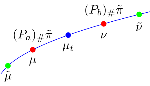
Figure 1: The measures $\tilde{\mu}$ and $\tilde{\nu}$ have the capacity to represent any barycenter $\mu_{t}$ of $\mu=(P_{a})_{\#}\tilde{\pi}$, $\nu=(P_{b})_{\#}\tilde{\pi}$, but they do it in a manner that our geometric sparse regularizer penalizes.

Theorem 1.

Consider measures $\mu,\nu,\tilde{\nu}$ with respective optimal transportation plans $\pi$ and $\tilde{\pi}$ and suppose $(\mu,\tilde{\nu})\in M(\mu,\nu)$. Let $\mu_{t}=(P_{t})_{\#}\pi$ be in the McCann interpolation between $\mu$ and $\nu$, and let $s$ be the associated time coordinate such that $(P_{s})_{\#}\tilde{\pi}=(P_{t})_{\#}\pi$. Then

$$(1-t)W_{2}^{2}(\mu,\mu_{t})+tW_{2}^{2}(\nu,\mu_{t})\leq(1-s)W_{2}^{2}(\mu,\mu_{t})+sW_{2}^{2}(\tilde{\nu},\mu_{t}).$$

With this, we can establish that subject to the constraint of perfect reconstruction (quantified by $M(\mu,\nu)$), minimizing the geometric sparse regularizer yields a unique solution that coincides with the true generating atoms in the case of all observed data lying on a McCann interpolation.

Corollary 1.

Let $\mu\neq\nu$ be two measures with optimal transport plan $\pi$. For any $(\tilde{\mu},\tilde{\nu})\in M(\mu,\nu)$, let $\tilde{\pi}$ be the associated optimal transport plan. Then for any barycenter $\mu_{t}=(P_{t})_{\#}\pi$ generated by $\mu,\nu$,

$$(\mu,\nu)=\operatorname*{arg\,min}_{\begin{subarray}{c}(\tilde{\mu},\tilde{\nu})\in M(\mu,\nu),\\ s\ s.t.(P_{s})_{\#}\tilde{\pi}=\mu_{t}\end{subarray}}(1-s)W_{2}^{2}(\tilde{\mu},\mu_{t})+sW_{2}^{2}(\tilde{\nu},\mu_{t}).$$

Proof.

Apply Theorem 1 twice, the second time after reversing parameterization. ∎

In other words, among all pairs of measures that contain the geodesic between the original data generators $\mu$ and $\nu$, the geometric sparse regularizer for every data point is minimized by $(\mu,\nu)$.

4 Proposed Algorithm

Optimization in Wasserstein space has been infeasible outside of problems with low-dimensional distributions due to the computational complexities of solving the transport problems (Bonneel et al.,, 2016). We make two primary design choices to make a tractable algorithm:

Shared Fixed Support:

We assume all measures lie on the same fixed finite support $\{\mathbf{x}_{i}\}_{i=1}^{N}\subset\mathbb{R}^{d}$. So, each distribution $\mu$ can be represented as a probability distribution $\mathbf{a}\in\Delta^{N}$ via $\mu=\sum_{i=1}^{N}a_{i}\delta_{\mathbf{x}_{i}}$. We will abuse notation and write $\mu$ in place of $\mathbf{a}$ when referring to discrete measures. Having a fixed support enables us to compute the pairwise costs $\|\mathbf{x}_{i}-\mathbf{x}_{j}\|_{2}^{2}$ upfront, which are used repeatedly in the transport and barycenter computations.

Entropic Regularization:

We use the entropically regularized Wasserstein distance (Cuturi,, 2013; Peyré et al.,, 2019). Simply stated, we can get simple and relatively cheap estimates of the Wasserstein distance by a few iterations of the Sinkhorn matrix scaling algorithm. We refer the reader to the aforementioned references for detailed discussion of the entropic regularization and it’s effect on computation; in brief it is repeated matrix-vector multiplications done with the kernel matrix $\mathbf{K}:=\exp(-\mathbf{C}/\varepsilon)$ where $\mathbf{C}\in\mathbb{R}^{N\times N}$ is the pairwise cost matrix formed from the support. Unsurprisingly, entropic regularization lends to a similar Sinkhorn-like iterative method to compute barycenters (Benamou et al.,, 2015); both methods can be derived as Bregman iterations. We make extensive use of automatic differentiation (Paszke et al.,, 2019) to handle variable updates. For all transport computations one could also use the unbiased Sinkhorn divergences instead (Feydy et al.,, 2019); we choose not to in order to compare directly to WDL.

Our main algorithm, which we call Geometrically Sparse Wasserstein Dictionary Learning (GeoSWDL), is detailed in Algorithm 1. Following the original WDL formulation of Schmitz et al., (2018), we optimize over arbitrary vectors in Euclidean space that each represent a unique probability distribution (both for atoms and barycentric weights) via softmax as a change of variables.

Algorithm 1 Geometrically Sparse Wasserstein Dictionary Learning (GeoSWDL)

1:Input: Training data $\{\mu_{i}\}_{i=1}^{n}\subset\Delta^{N}$, $L$, $\verb|optimizer|$

2:Initialize variables $\boldsymbol{\alpha}^{(0)}\in\mathbb{R}^{n\times m},\ \boldsymbol{\beta}^{(0)}\in\mathbb{R}^{m\times N}$ $\triangleright$ Use any initialization method

3:for $k\leftarrow 1,\ldots,L$ do

4:     loss $\leftarrow 0$ $\triangleright$ Set loss to zero for each iteration

5:     $\mathcal{D}^{(k)}\leftarrow\operatorname{CoV}(\boldsymbol{\alpha})$, $\mathbf{\Lambda}^{(k)}\leftarrow\operatorname{CoV}(\boldsymbol{\beta})$ $\triangleright$ Get updated dictionary/weights

6:     loss $\leftarrow\mathcal{F}(\mathcal{D}^{(k)},\mathbf{\Lambda}^{(k)},\{\mu_{i}\}_{i=1}^{n})$ $\triangleright$ Compute the objective function

7:     loss.backward() $\triangleright$ Compute the gradients with automatic differentiation

8:     Update $\boldsymbol{\alpha}^{(k)},\boldsymbol{\beta}^{(k)}$ with optimizer.step() $\triangleright$ Update variables

9:end for

10:Output: $\mathcal{D}^{(L)},\mathbf{\Lambda}^{(L)}$

We briefly describe initialization options for the algorithm:

Atom Initialization:

We consider 3 methods of initialization for the atoms: (i) uniform at random samples from $\Delta^{N}$; (ii) uniform at random data samples: pick $m$ of the data used to learn the dictionary as the initialization; (iii) $k$-means++ initialization: follow the initialization procedure of $k$-means++ algorithm using Wasserstein distances (Arthur and Vassilvitskii,, 2006) and use those choices as the initial atoms. We expect the data-based initialization schemes to converge faster and to better solutions, particularly with geometric sparse regularizer since the probability distributions that resemble the data will be favored, as we assume generating probability distributions should resemble the data to some degree.

Weight Initialization:

We consider 3 methods of initialization for the weights: (i) uniform at random samples from $\Delta^{m}$; (ii) Wasserstein histogram regression (Bonneel et al.,, 2016) to match each data point to the initialized atoms; (iii) estimating weights using the quadratic program described by Werenski et al., (2022); details of this approach are in the Supplementary Materials. Empirically, atom initialization was more important than the choice of weight initialization; we use method (i) for all experiments in Section 5.

Runtime Complexity:

To understand the complexity of our algorithm we focus on the complexity of a single iteration in the loop of Algorithm 1. We run a fixed number of Sinkhorn iterations, $L_{s}$, for both entropic distance computations as well as entropic barycenter computations. Thus, for a single data point the cost to compute the barycenter is $O(L_{s}N^{2}m)$ as each iteration of the Bregman projection is a matrix multiplication with the kernel. Similarly the computational cost of the loss is $O(L_{s}N^{2}+L_{s}N^{2}m)=O(L_{s}N^{2}m)$ (entropic distance between barycenter and true data point plus geometric sparse regularizer). With automatic differentiation the cost is the same as computing the values. Thus when considering all the data the cost per iteration is $O(nL_{s}N^{2}m)$. One could batch the data for simpler iterations, but we do not evaluate the effects of such a choice. The bottleneck cost is the matrix-vector operations in the Sinkhorn iterations; to circumvent this, particularly for larger problems, one could form a Nyström approximation of the kernel matrix (Altschuler et al.,, 2019). Geometric structure in the support, as is the case with data supported on a grid (e.g., images), can be leveraged to reduce computational burdens (Solomon et al.,, 2015).

5 Experiments

This section summarizes experiments on image and NLP data; further discussion is in the Supplementary Materials.

5.1 Identifying Generating Distributions With Synthetic MNIST Data

We demonstrate the utility of our geometric sparse regularizer in identifying the generating probability distributions in a generative model. In this experiment, we randomly select 3 samples from each MNIST (LeCun,, 1998) data class {0,1,2,…,9}. For each of the classes, we use the 3 samples to generate 50 synthetic samples by forming barycenters constructed with weights sampled uniformly from $\Delta^{3}$. This yields 500 total training points, each of which is a synthetic MNIST digit generated from a total of $3\times 10=30$ real MNIST digits. We then train a dictionary to learn 30 atoms. An optimal solution is to learn the original generating set of 30 distributions.

We run Algorithm 1 for $L=250$ iterations and use the Adam optimizer learning rate of 0.25 (other parameters left as default in PyTorch). For all Sinkhorn computations, we used 50 iterations. We compare the effects of geometric sparse regularization by varying the regularization parameter $\rho\in\{10^{-3},10^{-1},10^{1}\}$. Atoms are initialized using the K-means++ initialization. After learning the dictionary, we match the learned atoms to the true atoms by finding the assignment that minimizes transport cost between learned and true atoms. We solve the non-entropically regularized transport problem to ensure non-negative assignment costs. We visualize the learned vs. true atoms as well as a confusion matrix that demonstrates how well learned coefficients and atoms align with the true class in Figure 2.

As observed empirically in Figure 2 (b), increasing $\rho$ only helps the learned coefficients to be placed more correctly on their class after matching the atoms. This illustrates a trade-off associated with increasing $\rho$: more geometric sparse regularization may help the data be classified correctly, but the learned atoms may not resemble the true generating atoms as well. Indeed, in Figure 2 (c) we see that increasing $\rho$ concentrates the coefficients, as we would expect given the connection between GeoSWDL with large $\rho$ and Wasserstein $K$-means discussed in Section 3. We also note that as seen in Figure 2 (a), some of learned atoms for classes $\{1,2,6\}$ are less visually interpretable; this is due in part to the fact that during the optimization process, none of the training data use these atoms for their barycentric reconstruction. As such, the algorithm loses information about how to optimize those data points—they are effectively never updated because they are never used in reconstruction. A simple workaround we use is to restart the algorithm several times and select an output that places some weight on each atom (i.e. $\forall j,\exists i$ such that $(\boldsymbol{\lambda}_{i})_{j}\gg 0$).

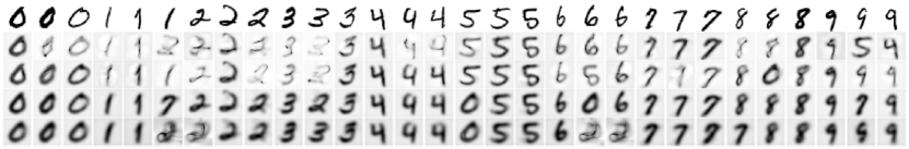
(a) Top row shows the true generating probability distributions. Subsequent rows show learned atoms with increasing $\rho$, after alignment.

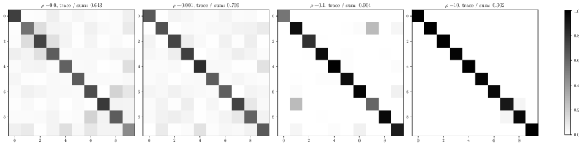
(b) The amount of mass assigned to weights of class $i$ to atoms of class $j$

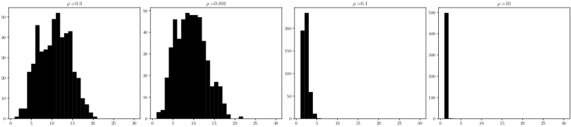
(c) The counts of minimal number of atoms needed to assign at least 95% of the mass in the barycenter as a proxy for sparsity

Figure 2: The learned digits shown are most interpretable in the moderate regularization regime (e.g., $\rho>0$ but not too large). As $\rho$ increases, (b) shows the concentration of coefficient energy on atoms that belong to the same class as the test data point, with atoms assigned by finding their closest training data. Moreover, we see in (c) that increasing $\rho$ increases the sparsity of the coefficients learned.

5.2 Learned Coefficients as Features for Document Classification

Here we demonstrate the effectiveness of the geometric sparse regularizer when used for a classification task comparing word documents. We represent documents as probability distributions with a bag-of-words (i.e. a vector of counts for each word in the document normalized to lie in the probability simplex) approach where we use learned embeddings of the words from Huang et al., (2016) as the support. The documents considered come from the BBCSPORT dataset which consists of 737 documents with 5 classes overall. We follow the experimental setup of Werenski et al., (2022), where a fixed number of random reference documents from each class were used. We instead learn a fixed size dictionary for each reference class. The documents used for training the dictionary are disjoint from the randomly selected documents used for comparison. We train each dictionary with a number of samples proportional to the size of the dictionary; for a dictionary of $m$ atoms we use $4m$ training samples. Since the dictionary atoms must have fixed support, we fix the support as the union of words present in the training documents.

For evaluation, we sample 100 random documents disjoint from the dictionary training sets and the randomly selected reference documents for baseline comparison, and classify them using the methods described below. Both the dictionaries and sets of random reference documents have the same number of elements per class and this number is varied from 1 to 12. We repeat this test 30 times and report results averaged across these trials. The results are visualized in Figures and 3 and 4.

We note that these plots compare against two baselines in terms of what generating measures to use: (i) random samples from the data; (ii) WDL, which corresponds to $\rho=0$ in the GeoSWDL framework.

Classification Methods: We state the 5 classification methods we consider on the learned coefficients.

1. 1-Nearest Neighbor (1NN): classifies based on the class of the nearest reference document in $W_{2}^{2}$;

2. Minimum Average Distance (MAD): selects the class with reference documents on average $W_{2}^{2}$-closest to the test document;

3. Minimum Barycentric Loss (MBL): we learn the barycentric weights to represent the test document by solving the quadratic program in Werenski et al., (2022) for each reference class. We then compute the barycentric representation for each class and classify with the one that minimizes $W_{2}^{2}$ to the test document;

4. Minimum Barycenter Loss (MBL-QP): selects the class that minimizes the aforementioned quadratic program’s objective value (a proxy for the $W_{2}^{2}$ distance between the barycentric representation and test document);

5. Maximum Coordinate (MC): also solves the aforementioned quadratic program to estimate barycentric weights when using the reference documents of all classes to represent the test document. The class is then assigned based on the class whose total portion of the estimated weights is largest.

We notice that at all levels of geometric sparse regularizer tested, learned dictionaries enable the barycenter focused methods to outperform all methods that use random samples of the data. Perhaps more interestingly, we note that increasing levels of geometric sparse regularization increases the performance of the simpler methods of 1NN and MAD. This suggests that the geometric sparse regularizer is promoting dictionary atoms that are more informative generally as individual atoms as opposed to the information contained in their collective representational capacity. As mentioned in the discussion of the geometric sparse regularizer in Section 3, the unregularized WDL objective is minimized by the dictionary probability distributions only with respect of their representative ability. On the other hand, as demonstrated here, GeoSWDL encourages the learned atoms to be informative themselves about the data they model, even generalizing to unseen data.

(a) 1NN

(b) MAD

(c) MBL

(d) MBL-QP

(e) MC

Figure 3: Accuracy vs. number of reference documents. Solid lines and dashed lines correspond to the reference documents being learned dictionary atoms or random documents from each class, respectively. Here, we group by method and show the impact of different levels of regularization and learning versus random atoms. Except for small $\rho$ in 1NN, using learned reference documents significantly outperforms the use randomly sampled documents across all number of references.

(a) $\rho=0$

(b) $\rho=0.01$

(c) $\rho=0.1$

(d) $\rho=1.0$

(e) $\rho=10.0$

Figure 4: Accuracy vs. number of reference documents. Solid lines and dashed lines correspond to the reference documents being learned dictionary atoms or random documents from each class respectively. Here, we group by regularization parameter and show the impact of different methods and learning versus random atoms. Increasing $\rho$ brings the non-barycentric based methods to performance parity with the barycentric based classification approaches.

6 Conclusion

We have extended the WDL framework by introducing a geometric sparse regularizer that interpolates between WDL and Wasserstein $K$-means according to a tuneable parameter $\rho$. We have shown the geometric sparse regularizer itself is useful in solving uniqueness and identifiability problems relating to the dictionary and weights, by leveraging characterizations of the nonlinear problem of exact barycentric reconstruction as well as geometric properties of Wasserstein geodesics. Additionally, we have shown the usefulness of our extension in providing improvements to classification methods on real data. In particular our regularized framework improves over classical WDL in terms of atom interpretability and performance in classification.

Future Work: Computational runtime remains a burden for both GeoSWDL and classical WDL. While automatic differentiation provides for simple implementations, there may exist more specific algorithms to the dictionary learning framework; in particular the use of the geometric sparse regularizer may enable faster algorithms as is done in the linear case (Mallat and Zhang,, 1993). Relatedly, notions of linear optimal transport have important computational potential (Wang et al.,, 2013; Moosmüller and Cloninger,, 2020; Hamm et al.,, 2022) in speeding up runtime of $W_{2}^{2}$ pairwise calculations for certain classes of measures.

The analysis of the sparse coding step in Section 3 does not immediately extend to case when the dictionary $\mathcal{D}$ is changing (which causes $\mathbf{A}$ to change). Understanding how the matrix $\mathbf{A}$ changes with $\mathcal{D}$ is a topic of ongoing research, and may allow for a closed-form solution to (6). Relatedly, Theorem 1 applies only to the case when the original data lie exactly on a Wasserstein barycenter between $m=2$ distributions; extending to $m\geq 3$ is a topic of ongoing research.

Acknowledgements: We thank Demba Ba, JinCheng Wang, and Matt Werenski for insightful discussions. MM was partially supported was partially supported by NSF DMS 1924513 and CCF-1934553. SA was partially supported by NSF CCF 1553075, NSF DRL 1931978, NSF EEC 1937057, and AFOSR FA9550-18-1-0465. JMM was partially supported by NSF DMS 1912737, NSF DMS 1924513, and The Camille & Henry Dreyfus Foundation. AT was partially supported by DMS 2208392. The authors acknowledge the Tufts University High Performance Compute Cluster (https://it.tufts.edu/high-performance-computing) which was utilized for the research reported in this paper.

Appendix A Precise Statement and Proof of Proposition 1

In order to establish this result, it is essential to note that if measures $\mu$ and $\nu$ satisfy the constraints that they have finite second moments and do not give mass to small sets (e.g., are absolutely continuous) (Villani,, 2021), their optimal plan $\pi^{*}$ concentrates on the graph of $T^{*}=\nabla\phi$ for a strictly convex $\phi$, so that

$$W_{2}^{2}(\mu,\nu)=\displaystyle\int_{\mathbb{R}^{d}}\|T^{*}(\mathbf{x})-\mathbf{x}\|_{2}^{2}d\mu(\mathbf{x})$$

where $T^{*}$ satisfies the pushforward constraint $T^{*}_{\#}\mu=\nu$ and is called the optimal transport map (Smith and Knott,, 1987; Brenier,, 1991).

In order to precisely state Proposition 1, we require a few regularity assumptions A1-A3 on the dictionary $\mathcal{D}=\{\mathcal{D}_{j}\}_{j=1}^{m}$ and measure $\mu$. These are required to invoke Theorem 1 in Werenski et al., (2022), which characterizes exactly when

$$\mu=\operatorname{Bary}(\mathcal{D},\boldsymbol{\lambda})$$

for some $\boldsymbol{\lambda}\in\Delta^{m}$.

A1:  The measures $\{\mathcal{D}_{j}\}_{j=1}^{m}$ and $\mu$ are absolutely continuous and supported on either all of $\mathbb{R}^{d}$ or a bounded open convex subset. Call this shared support set $\Omega$.

A2:  The measures $\{\mathcal{D}_{j}\}_{j=1}^{m}$ and $\mu$ have respective densities $\{g_{j}\}_{j=1}^{m}$ and $g$ which are bounded above and $g_{1},...,g_{m}$ are strictly positive on $\Omega$.

A3:  If $\Omega=\mathbb{R}^{d}$ then $\{g_{j}\}_{j=1}^{m}$ and $g$ are locally Hölder continuous. Otherwise $\{g_{j}\}_{j=1}^{m}$ and $g$ are bounded away from zero on $\Omega$.

Proposition 2.

Let $\mu$ be fixed and let $\{\mathcal{D}_{j}\}_{j=1}^{m}\subset\mathcal{P}(\mathbb{R}^{d})$ be a fixed dictionary. Consider

$$\underset{\boldsymbol{\lambda}\in\Delta^{m}}{\arg\min}\,\,\sum_{j=1}^{m}\lambda_{j}W_{2}^{2}(\mathcal{D}_{j},\mu)\,\,\emph{subject to}\,\,\mu=\operatorname{Bary}(\mathcal{D},\boldsymbol{\lambda}).$$ (9)

If $\mathcal{D}$ and $\mu$ satisfy the assumptions A1-A3, the solution to (9) is given by

$$\underset{\boldsymbol{\lambda}\in\Delta^{m}}{\arg\min}\,\,\boldsymbol{\lambda}^{T}\mathbf{c}\,\,\emph{subject to}\,\,\mathbf{A}\boldsymbol{\lambda}=\mathbf{0},$$ (10)

where $\mathbf{c}$ and $\mathbf{A}\in\mathbb{R}^{m\times m}$ are uniquely determined by $\mu,\{\mathcal{D}_{j}\}_{j=1}^{m}$.

Proof.

Let $\{T_{j}\}_{j=1}^{m}$ be the optimal transport maps between $\mu$ and $\mathcal{D}_{j}$. Define $\mathbf{A}\in\mathbb{R}^{m\times m}$ by

$$A_{j\ell}=\int_{\mathbb{R}^{d}}\langle T_{j}(\mathbf{x})-\mathbf{x},T_{\ell}(\mathbf{x})-\mathbf{x}\rangle d\mu(\mathbf{x}).$$

Then by Theorem 1 in Werenski et al., (2022), which holds because A1-A3 hold,

$$\mu=\operatorname{Bary}(\mathcal{D},\boldsymbol{\lambda})\Longleftrightarrow\boldsymbol{\lambda}^{T}\mathbf{A}\boldsymbol{\lambda}=0.$$

Since $\mathbf{A}$ is symmetric and positive semidefinite (it is in fact a Gram matrix), $\boldsymbol{\lambda}^{T}\mathbf{A}\boldsymbol{\lambda}=0$ is equivalent to $\mathbf{A}\boldsymbol{\lambda}=\mathbf{0}$. Letting $\mathbf{c}$ be defined as $c_{j}=W_{2}^{2}(\mathcal{D}_{j},\mu)$ gives the result. ∎

Appendix B Proof of Theorem 1

Proof.

Rearranging, we aim to show

$$0\leq(t-s)W_{2}^{2}(\mu,\mu_{t})+sW_{2}^{2}(\mu_{t},\tilde{\nu})-tW_{2}^{2}(\mu_{t},\nu).$$

Noting that McCann interpolants are in fact constant-speed geodesics in Wasserstein space (Ambrosio et al.,, 2005), we have that

$$t=\frac{W_{2}(\mu,\mu_{t})}{W_{2}(\mu,\nu)},\quad s=\frac{W_{2}(\mu,\mu_{t})}{W_{2}(\mu,\tilde{\nu})}$$

and

$$W_{2}(\mu,\tilde{\nu}) =W_{2}(\mu,\nu)+W_{2}(\nu,\tilde{\nu}),$$

$$W_{2}(\mu_{t},\tilde{\nu}) =W_{2}(\mu_{t},\nu)+W_{2}(\nu,\tilde{\nu}).$$

In particular, $s<t$ and so it suffices to show

$$tW_{2}^{2}(\mu_{t},\nu) \leq sW_{2}^{2}(\mu_{t},\tilde{\nu})$$

$$\Longleftrightarrow\frac{W_{2}(\mu,\mu_{t})}{W_{2}(\mu,\nu)}W_{2}^{2}(\mu_{t},\nu) \leq\frac{W_{2}(\mu,\mu_{t})}{W_{2}(\mu,\tilde{\nu})}W_{2}^{2}(\mu_{t},\tilde{\nu})$$

$$\Longleftrightarrow\frac{W_{2}^{2}(\mu_{t},\nu)}{W_{2}(\mu,\nu)} \leq\frac{W_{2}^{2}(\mu_{t},\tilde{\nu})}{W_{2}(\mu,\tilde{\nu})}$$

$$\Longleftrightarrow\frac{W_{2}^{2}(\mu_{t},\nu)}{W_{2}(\mu,\nu)} \leq\frac{(W_{2}(\mu_{t},\nu)+W_{2}(\nu,\tilde{\nu}))^{2}}{W_{2}(\mu,\nu)+W_{2}(\nu,\tilde{\nu})}$$

$$\Longleftrightarrow W_{2}^{2}(\mu_{t},\nu)(W_{2}(\mu,\nu)+W_{2}(\nu,\tilde{\nu})) \leq W_{2}(\mu,\nu)(W_{2}(\mu_{t},\nu)+W_{2}(\nu,\tilde{\nu}))^{2}$$

$$\Longleftrightarrow W_{2}^{2}(\mu_{t},\nu)(W_{2}(\mu,\nu)+W_{2}(\nu,\tilde{\nu})) \leq W_{2}(\mu,\nu)(W_{2}^{2}(\mu_{t},\nu)+2W_{2}(\mu_{t},\nu)W_{2}(\nu,\tilde{\nu})+W_{2}^{2}(\nu,\tilde{\nu}))$$

$$\Longleftrightarrow W_{2}^{2}(\mu_{t},\nu)W_{2}(\nu,\tilde{\nu}) \leq W_{2}(\mu,\nu)(2W_{2}(\mu_{t},\nu)W_{2}(\nu,\tilde{\nu})+W_{2}^{2}(\nu,\tilde{\nu})).$$

If $\tilde{\nu}=\nu$, the result follows trivially. So, assume $W_{2}(\nu,\tilde{\nu})>0$. Then the above reduces to

$$W_{2}^{2}(\mu_{t},\nu)\leq W_{2}(\mu,\nu)(2W_{2}(\mu_{t},\nu)+W_{2}(\nu,\tilde{\nu})).$$

The result follows by noting that $W_{2}(\mu_{t},\nu)\leq W_{2}(\mu,\nu)$ and that $W_{2}(\nu,\tilde{\nu})\geq 0$. ∎

Appendix C Experimental Details

For each of the experiments we report specific parameters used to generate the results. We also report the timings based on our (not necessarily optimal) code.

C.1 MNIST

Specific parameter choices:

• Atom initialization: Wasserstein K-Means++.

• Weight initialization: Uniform samples from the simplex.

• Optimizer: Adam with default parameters except for learning rate as 0.25.

• We use $L=250$ iterations for reasonable convergence.

• We use $L_{s}=50$ Sinkhorn iterations for both Wasserstein distance and barycenter computations.

• Entropic transport computations were accelerated with Convolutional Wasserstein (Solomon et al.,, 2015).

This experiment took 8 hours total using all cpu cores of an Apple M1 chip (no gpu).

C.2 NLP

We plot the 1 standard deviation bars for the NLP experiments in Figure LABEL:fig:nlp-std. Specific parameter choices:

• Atom initialization: Wasserstein K-Means++.

• Weight initialization: Each weight is initialized as a vector with uniform random samples and then normalized to lie on the simplex. This differs from uniform samples from the simplex, but in practice there were no performance differences.

• Optimizer: Adam with default parameters except for learning rate as 0.25.

• We use $L=300$ iterations for reasonable convergence.

• We use $L_{s}=25$ Sinkhorn iterations for both Wasserstein distance and barycenter computations.

Running one of the thirty trials of the experiment for all number of the references took at most 2 days on an HPC node using 2 cpu cores and one Nvidia gpu of type T4, RTX 6000, V100, or P100 (depending on node availability).

References

- Agueh and Carlier, (2011) Agueh, M. and Carlier, G. (2011). Barycenters in the wasserstein space. SIAM Journal on Mathematical Analysis, 43(2):904–924.
- Aharon et al., (2006) Aharon, M., Elad, M., and Bruckstein, A. (2006). K-svd: An algorithm for designing overcomplete dictionaries for sparse representation. IEEE Transactions on signal processing, 54(11):4311–4322.
- Altschuler et al., (2019) Altschuler, J., Bach, F., Rudi, A., and Niles-Weed, J. (2019). Massively scalable sinkhorn distances via the nyström method. Advances in neural information processing systems, 32.
- Ambrosio et al., (2005) Ambrosio, L., Gigli, N., and Savaré, G. (2005). Gradient flows: in metric spaces and in the space of probability measures. Springer Science & Business Media.
- Arthur and Vassilvitskii, (2006) Arthur, D. and Vassilvitskii, S. (2006). k-means++: The advantages of careful seeding. Technical report, Stanford.
- Barlow et al., (1961) Barlow, H. B. et al. (1961). Possible principles underlying the transformation of sensory messages. Sensory communication, 1(01).
- Belkin and Niyogi, (2003) Belkin, M. and Niyogi, P. (2003). Laplacian eigenmaps for dimensionality reduction and data representation. Neural computation, 15(6):1373–1396.
- Benamou et al., (2015) Benamou, J.-D., Carlier, G., Cuturi, M., Nenna, L., and Peyré, G. (2015). Iterative bregman projections for regularized transportation problems. SIAM Journal on Scientific Computing, 37(2):A1111–A1138.
- Berry et al., (2007) Berry, M. W., Browne, M., Langville, A. N., Pauca, V. P., and Plemmons, R. J. (2007). Algorithms and applications for approximate nonnegative matrix factorization. Computational statistics & data analysis, 52(1):155–173.
- Bigot et al., (2017) Bigot, J., Gouet, R., Klein, T., and López, A. (2017). Geodesic pca in the wasserstein space by convex pca. Annales de l’Institut Henri Poincaré, Probabilités et Statistiques, 53(1):1–26.
- Boissard et al., (2015) Boissard, E., Le Gouic, T., and Loubes, J.-M. (2015). Distribution’s template estimate with wasserstein metrics. Bernoulli, 21(2):740–759.
- Bonneel et al., (2016) Bonneel, N., Peyré, G., and Cuturi, M. (2016). Wasserstein barycentric coordinates: histogram regression using optimal transport. ACM Trans. Graph., 35(4):71–1.
- Brenier, (1991) Brenier, Y. (1991). Polar factorization and monotone rearrangement of vector-valued functions. Communications on pure and applied mathematics, 44(4):375–417.
- Cai et al., (2010) Cai, D., He, X., Han, J., and Huang, T. S. (2010). Graph regularized nonnegative matrix factorization for data representation. IEEE transactions on pattern analysis and machine intelligence, 33(8):1548–1560.
- Cherian and Sra, (2016) Cherian, A. and Sra, S. (2016). Riemannian dictionary learning and sparse coding for positive definite matrices. IEEE transactions on neural networks and learning systems, 28(12):2859–2871.
- Coifman and Lafon, (2006) Coifman, R. R. and Lafon, S. (2006). Diffusion maps. Applied and computational harmonic analysis, 21(1):5–30.
- Cutler and Breiman, (1994) Cutler, A. and Breiman, L. (1994). Archetypal analysis. Technometrics, 36(4):338–347.
- Cuturi, (2013) Cuturi, M. (2013). Sinkhorn distances: Lightspeed computation of optimal transport. Advances in neural information processing systems, 26.
- Cuturi and Doucet, (2014) Cuturi, M. and Doucet, A. (2014). Fast computation of wasserstein barycenters. In International conference on machine learning, pages 685–693. PMLR.
- Domazakis et al., (2019) Domazakis, G., Drivaliaris, D., Koukoulas, S., Papayiannis, G., Tsekrekos, A., and Yannacopoulos, A. (2019). Clustering measure-valued data with wasserstein barycenters. arXiv preprint arXiv:1912.11801.
- Donoho, (2006) Donoho, D. L. (2006). Compressed sensing. IEEE Transactions on information theory, 52(4):1289–1306.
- Donoho et al., (1992) Donoho, D. L., Johnstone, I. M., Hoch, J. C., and Stern, A. S. (1992). Maximum entropy and the nearly black object. Journal of the Royal Statistical Society: Series B (Methodological), 54(1):41–67.
- Dornaika and Weng, (2019) Dornaika, F. and Weng, L. (2019). Sparse graphs with smoothness constraints: Application to dimensionality reduction and semi-supervised classification. Pattern Recognition, 95:285–295.
- Eckart and Young, (1936) Eckart, C. and Young, G. (1936). The approximation of one matrix by another of lower rank. Psychometrika, 1(3):211–218.
- Elad, (2010) Elad, M. (2010). Sparse and redundant representations: from theory to applications in signal and image processing. Springer.
- Engan et al., (2000) Engan, K., Aase, S. O., and Husoy, J. H. (2000). Multi-frame compression: Theory and design. Signal Processing, 80(10):2121–2140.
- Feydy et al., (2019) Feydy, J., Séjourné, T., Vialard, F.-X., Amari, S.-i., Trouvé, A., and Peyré, G. (2019). Interpolating between optimal transport and mmd using sinkhorn divergences. In The 22nd International Conference on Artificial Intelligence and Statistics, pages 2681–2690. PMLR.
- Guo et al., (2010) Guo, K., Ishwar, P., and Konrad, J. (2010). Action recognition using sparse representation on covariance manifolds of optical flow. In 2010 7th IEEE international conference on advanced video and signal based surveillance, pages 188–195. IEEE.
- Hamm et al., (2022) Hamm, K., Henscheid, N., and Kang, S. (2022). Wassmap: Wasserstein isometric mapping for image manifold learning. arXiv preprint arXiv:2204.06645.
- Harandi et al., (2013) Harandi, M., Sanderson, C., Shen, C., and Lovell, B. C. (2013). Dictionary learning and sparse coding on grassmann manifolds: An extrinsic solution. In Proceedings of the IEEE international conference on computer vision, pages 3120–3127.
- Harandi et al., (2015) Harandi, M. T., Hartley, R., Lovell, B., and Sanderson, C. (2015). Sparse coding on symmetric positive definite manifolds using bregman divergences. IEEE transactions on neural networks and learning systems, 27(6):1294–1306.
- Hotelling, (1933) Hotelling, H. (1933). Analysis of a complex of statistical variables into principal components. Journal of educational psychology, 24(6):417.
- Hromádka et al., (2008) Hromádka, T., DeWeese, M. R., and Zador, A. M. (2008). Sparse representation of sounds in the unanesthetized auditory cortex. PLoS biology, 6(1):e16.
- Huang et al., (2016) Huang, G., Guo, C., Kusner, M. J., Sun, Y., Sha, F., and Weinberger, K. Q. (2016). Supervised word mover’s distance. Advances in neural information processing systems, 29.
- Kyrillidis et al., (2013) Kyrillidis, A., Becker, S., Cevher, V., and Koch, C. (2013). Sparse projections onto the simplex. In International Conference on Machine Learning, pages 235–243. PMLR.
- Larsson and Ugander, (2011) Larsson, M. and Ugander, J. (2011). A concave regularization technique for sparse mixture models. Advances in Neural Information Processing Systems, 24.
- LeCun, (1998) LeCun, Y. (1998). The mnist database of handwritten digits. http://yann. lecun. com/exdb/mnist/.
- Lee and Seung, (2000) Lee, D. and Seung, H. S. (2000). Algorithms for non-negative matrix factorization. Advances in neural information processing systems, 13.
- Lee and Seung, (1999) Lee, D. D. and Seung, H. S. (1999). Learning the parts of objects by non-negative matrix factorization. Nature, 401(6755):788–791.
- Li et al., (2020) Li, P., Rangapuram, S. S., and Slawski, M. (2020). Methods for sparse and low-rank recovery under simplex constraints. Statistica Sinica, 30(2):557–577.
- Li et al., (2008) Li, X., Hu, W., Zhang, Z., Zhang, X., Zhu, M., and Cheng, J. (2008). Visual tracking via incremental log-euclidean riemannian subspace learning. In 2008 IEEE Conference on Computer Vision and Pattern Recognition, pages 1–8. IEEE.
- Liu et al., (2018) Liu, T., Shi, Z., and Liu, Y. (2018). Kernel sparse representation on grassmann manifolds for visual clustering. Optical Engineering, 57(5):053104.
- Maggioni et al., (2016) Maggioni, M., Minsker, S., and Strawn, N. (2016). Multiscale dictionary learning: non-asymptotic bounds and robustness. The Journal of Machine Learning Research, 17(1):43–93.
- Mairal et al., (2011) Mairal, J., Bach, F., and Ponce, J. (2011). Task-driven dictionary learning. IEEE transactions on pattern analysis and machine intelligence, 34(4):791–804.
- Mallat, (1999) Mallat, S. (1999). A wavelet tour of signal processing. Elsevier.
- Mallat and Zhang, (1993) Mallat, S. G. and Zhang, Z. (1993). Matching pursuits with time-frequency dictionaries. IEEE Transactions on signal processing, 41(12):3397–3415.
- McCann, (1997) McCann, R. J. (1997). A convexity principle for interacting gases. Advances in mathematics, 128(1):153–179.
- Mehta and Gray, (2013) Mehta, N. and Gray, A. (2013). Sparsity-based generalization bounds for predictive sparse coding. In International Conference on Machine Learning, pages 36–44. PMLR.
- Moosmüller and Cloninger, (2020) Moosmüller, C. and Cloninger, A. (2020). Linear optimal transport embedding: Provable wasserstein classification for certain rigid transformations and perturbations. arXiv preprint arXiv:2008.09165.
- Olshausen and Field, (1996) Olshausen, B. A. and Field, D. J. (1996). Emergence of simple-cell receptive field properties by learning a sparse code for natural images. Nature, 381(6583):607–609.
- Olshausen and Field, (1997) Olshausen, B. A. and Field, D. J. (1997). Sparse coding with an overcomplete basis set: A strategy employed by v1? Vision research, 37(23):3311–3325.
- Paszke et al., (2019) Paszke, A., Gross, S., Massa, F., Lerer, A., Bradbury, J., Chanan, G., Killeen, T., Lin, Z., Gimelshein, N., Antiga, L., Desmaison, A., Kopf, A., Yang, E., DeVito, Z., Raison, M., Tejani, A., Chilamkurthy, S., Steiner, B., Fang, L., Bai, J., and Chintala, S. (2019). Pytorch: An imperative style, high-performance deep learning library. In Wallach, H., Larochelle, H., Beygelzimer, A., d'Alché-Buc, F., Fox, E., and Garnett, R., editors, Advances in Neural Information Processing Systems 32, pages 8024–8035. Curran Associates, Inc.
- Peyré et al., (2019) Peyré, G., Cuturi, M., et al. (2019). Computational optimal transport: With applications to data science. Foundations and Trends® in Machine Learning, 11(5-6):355–607.
- Rabin et al., (2011) Rabin, J., Peyré, G., Delon, J., and Bernot, M. (2011). Wasserstein barycenter and its application to texture mixing. In International Conference on Scale Space and Variational Methods in Computer Vision, pages 435–446. Springer.
- Roweis and Saul, (2000) Roweis, S. T. and Saul, L. K. (2000). Nonlinear dimensionality reduction by locally linear embedding. Science, 290(5500):2323–2326.
- Santambrogio, (2015) Santambrogio, F. (2015). Optimal transport for applied mathematicians. Birkäuser, NY, 55(58-63):94.
- Schmitz et al., (2018) Schmitz, M. A., Heitz, M., Bonneel, N., Ngole, F., Coeurjolly, D., Cuturi, M., Peyré, G., and Starck, J.-L. (2018). Wasserstein dictionary learning: Optimal transport-based unsupervised nonlinear dictionary learning. SIAM Journal on Imaging Sciences, 11(1):643–678.
- Scholkopf et al., (1997) Scholkopf, B., Smola, A., and Müller, K.-R. (1997). Kernel principal component analysis. In International conference on artificial neural networks, pages 583–588. Springer.
- Seguy and Cuturi, (2015) Seguy, V. and Cuturi, M. (2015). Principal geodesic analysis for probability measures under the optimal transport metric. Advances in Neural Information Processing Systems, 28.
- Shashanka et al., (2007) Shashanka, M., Raj, B., and Smaragdis, P. (2007). Sparse overcomplete latent variable decomposition of counts data. Advances in neural information processing systems, 20.
- Smith and Knott, (1987) Smith, C. S. and Knott, M. (1987). Note on the optimal transportation of distributions. Journal of Optimization Theory and Applications, 52(2):323–329.
- Solomon et al., (2015) Solomon, J., De Goes, F., Peyré, G., Cuturi, M., Butscher, A., Nguyen, A., Du, T., and Guibas, L. (2015). Convolutional wasserstein distances: Efficient optimal transportation on geometric domains. ACM Transactions on Graphics (ToG), 34(4):1–11.
- Tankala et al., (2020) Tankala, P., Tasissa, A., Murphy, J. M., and Ba, D. (2020). K-deep simplex: Deep manifold learning via local dictionaries. arXiv preprint arXiv:2012.02134.
- Tasissa et al., (2021) Tasissa, A., Tankala, P., and Ba, D. (2021). Weighed on the simplex: Compressive sensing meets locality. In 2021 IEEE Statistical Signal Processing Workshop (SSP), pages 476–480. IEEE.
- Tenenbaum et al., (2000) Tenenbaum, J. B., De Silva, V., and Langford, J. C. (2000). A global geometric framework for nonlinear dimensionality reduction. Science, 290(5500):2319–2323.
- Tuzel et al., (2006) Tuzel, O., Porikli, F., and Meer, P. (2006). Region covariance: A fast descriptor for detection and classification. In European conference on computer vision, pages 589–600. Springer.
- Tuzel et al., (2007) Tuzel, O., Porikli, F., and Meer, P. (2007). Human detection via classification on riemannian manifolds. In 2007 IEEE Conference on Computer Vision and Pattern Recognition, pages 1–8. IEEE.
- Verdinelli and Wasserman, (2019) Verdinelli, I. and Wasserman, L. (2019). Hybrid wasserstein distance and fast distribution clustering. Electronic Journal of Statistics, 13(2):5088–5119.
- Villani, (2021) Villani, C. (2021). Topics in optimal transportation, volume 58. American Mathematical Soc.
- Wang et al., (2013) Wang, W., Slepčev, D., Basu, S., Ozolek, J. A., and Rohde, G. K. (2013). A linear optimal transportation framework for quantifying and visualizing variations in sets of images. International journal of computer vision, 101(2):254–269.
- Werenski et al., (2022) Werenski, M. E., Jiang, R., Tasissa, A., Aeron, S., and Murphy, J. M. (2022). Measure estimation in the barycentric coding model. In International Conference on Machine Learning, pages 23781–23803. PMLR.
- Yin et al., (2016) Yin, M., Guo, Y., Gao, J., He, Z., and Xie, S. (2016). Kernel sparse subspace clustering on symmetric positive definite manifolds. In proceedings of the IEEE Conference on Computer Vision and Pattern Recognition, pages 5157–5164.
- Zhuang et al., (2022) Zhuang, Y., Chen, X., and Yang, Y. (2022). Wasserstein -means for clustering probability distributions. arXiv preprint arXiv:2209.06975.