Exact Holographic Tensor Networks – Constructing CFT_D from TQFT_D+1

Abstract

In this paper, inspired by Aasen et al. (2016, 2020); Vanhove et al. (2018), we proposed a class of lattice renormalization group (RG) operators, each operator determined by a topological order $T$ in $D+1$ space-time dimensions. Taking the overlap between an eigenstate $\langle\Omega|$ of the RG operator with the ground state wave-function $|\Psi\rangle$ of $T$ (i.e. $\langle\Omega|\Psi\rangle$) gives rise to partition functions of conformal (including topological) theories in $D$ dimensions with categorical symmetry related to $T$, realizing a holographic relation discussed in the literature explicitly. We illustrate this in explicit examples at $D=1,2,3$. Exact eigenstates of the RG operator can be solved explicitly from (higher) separable Frobenius algebra of the (higher) input fusion category $\mathcal{C}$ defining the lattice model of $T$, and they give the $D$ dimensional symmetric TQFTs. Eigenstates corresponding to actual conformal theories describe phase transitions between these topological fixed points. The critical points can be searched numerically (practically with truncated bond dimension) and we demonstrate that known critical couplings of $SU(2)_{k}$ integrable lattice models are numerically recovered from our procedure, alongside a curious tricritical point that we found at $k=4$. We demonstrate that the 2+1 D Ising model can also be obtained as a strange correlator with the associated $4D$ topological order being the 4D toric code. The numerical procedure that we devise to search for the 3D critical temperature is a novel tensor renormalization group algorithm, that fully harnesses the algebraic and geometric properties of the RG operator. Finally since the RG operator is in fact an exact analytic holographic tensor network, we compute “bulk-boundary” correlator and compare with the AdS/CFT dictionary. Promisingly, they are numerically compatible given our accuracy, although further works will be needed to explore the precise connection to the AdS/CFT correspondence.

I Introduction

In recent years, we have witnessed an explosion of activity in the study of generalization of the notion of global symmetries, loosely termed “categorical symmetry” Bhardwaj and Tachikawa (2018); Chang et al. (2019); Thorngren and Wang (2019, 2021); Ji and Wen (2020); Kong et al. (2020a); Albert et al. (2021); Chatterjee and Wen (2022a); Liu and Ji (2022); Lootens et al. (2021); Freed and Teleman (2018); Levin (2020), which was preceded by an extensive and systematic study of defects in rational conformal field theories in 2D Verlinde (1988); Petkova and Zuber (2001); Frohlich et al. (2007, 2004); Fuchs et al. (2002, 2004a, 2004b, 2005); Quella et al. (2007); Fuchs et al. (2008, 2007); Bachas and Brunner (2008); Davydov et al. (2011, 2015); Kong et al. (2021); Petkova (2010); Carqueville and Runkel (2016); Kitaev and Kong (2012); Brunner et al. (2014); Petkova (2013); Aasen et al. (2016); Williamson et al. (2017); Aasen et al. (2020); Vanhove et al. (2018); Makabe and Watts (2017); Thorngren (2020); Ji et al. (2020); Lin and Shao (2021); Chang and Lin (2021); Huang et al. (2021a); Burbano et al. (2021) and topological field theories Davydov et al. (2011); Carqueville and Runkel (2016); Brunner et al. (2015); Carqueville et al. (2020, 2019). It has been applied to constrain theories and renormalization group flows Chang et al. (2019); Thorngren and Wang (2019); Komargodski et al. (2021); Thorngren and Wang (2021); Kikuchi (2021); Rudelius and Shao (2020); Heidenreich et al. (2021); McNamara (2021); Cordova et al. (2022); Arias-Tamargo and Rodriguez-Gomez (2022). Categorical symmetry usually refers to the algebra of topological defects in a quantum theory, and group symmetry is a special case. In Ji and Wen (2020) categorical symmetry particularly refers to the enlarged collection of symmetries generated by the charges together with gauge fluxes which appear when the symmetry is gauged. This consideration of enlarged symmetry leads to a very general holographic relation. It has been suggested that to describe a $D$ dimensional system $S$ with topological defects associated to a tensor category $\mathcal{C}$, the system $S$ can be associated to a boundary condition of a topological theory in $D+1$ dimensions that is described by the center of $\mathcal{C}$ denoted $\mathcal{Z}(\mathcal{C})$, and whose topological excitations include the complete set of charges and fluxes Freed and Teleman (2018); Lootens et al. (2021); Ji and Wen (2020); Kong et al. (2020a); Albert et al. (2021); Chatterjee and Wen (2022a, b); Liu and Ji (2022); Kong and Zheng (2018, 2020, 2021, 2022); Kong et al. (2020b, 2022); Xu and Zhang (2022); Aasen et al. (2016); Vanhove et al. (2018); Lootens et al. (2019); Gaiotto and Kulp (2021); Bhardwaj et al. (2020); Apruzzi et al. (2021); Moradi et al. (2022).

Separately, it is observed that infinite classes of well known $2$-dimensional critical partition functions of integrable statistical models can be expressed as the overlap between the ground state wave-functions $|\Psi\rangle$ of topological orders in 2+1 D and some carefully chosen state $\langle\Omega|$ Aasen et al. (2020); Vanhove et al. (2018); Lootens et al. (2019); Vanhove et al. (2021), often called a “strange correlator”. The choice of the topological order associated to a modular higher category $\mathcal{C}$ captures the categorical symmetry of the critical model constructed, while $\langle\Omega|$ is chosen by making comparison with known lattice models, or via some educated guesses. This method has been applied to construct the partition function of a novel CFT believed to exist Vanhove et al. (2021); Huang et al. (2021b), whose categorical symmetry is related to the Haaegerup category.

We believe this is an explicit realization of the holographic principle mentioned above that applies way more generally than $D=2$ CFTs and $D+1=3$ TQFTs. As such, our paper achieved two goals.

First, we generalize the strange correlator construction to arbitrary dimensions (explicitly for $1\leq D\leq 3$), and give a more systematic way of constructing these partition functions and searching for critical points. Our method is based on understanding the nature of $\langle\Omega|$. We show that one can construct a renormalization group (RG) operator as a holographic tensor network that is purely specified by the category $\mathcal{C}$ associated to a categorical symmetry $\mathcal{Z}(\mathcal{C})$. The operator is constructed by considering coarse graining the topological wave-function $|\Psi\rangle$ . A necessary condition for $\langle\Omega|\Psi\rangle$ to represent the partition function of a conformal theory is that $\langle\Omega|$ is an eigenstate of the RG operator. Essentially, obtaining conformal theories in $D$ dimensions (of which topological theories form a sub-class) that carry categorical symmetry $\mathcal{Z}(\mathcal{C})$ is equivalent to obtaining eigenstates of the RG operator determined by a topological order in $D+1$ dimensions. We found that every Frobenius algebra of the input fusion category $\mathcal{C}$ (such that its center is $\mathcal{Z}(\mathcal{C})$) defining the $D+1$ dimensional lattice topological model corresponds to an eigenstate of the RG operator, and produces a symmetric TQFT in $D$ dimensions. The CFT is located at the phase transition points between these TQFT’s. The boundary condition approximating a CFT can be found by interpolating between a pair of boundary conditions characterized by two Frobenius algebra, between which there is a phase transition point. Away from the conformal fixed point, repeated use of the RG operator would instead generate for us a Frobenius algebra of the fusion category $\mathcal{C}$. We note that along the way of practically implementing the flow of 3D partition functions under repeated use of the RG operator numerically, we essentially develop an explicit tensor renormalization group algorithm Levin and Nave (2007), now generalized to 3D. Second, we notice the similarity between the current holographic tensor network and the p-adic CFT tensor network we constructed in Hung et al. (2019); Chen et al. (2021a, b). The later of which is made up of tensors constructed from the (co-) product of an associative algebra determined by the operator fusion algebra of the p-adic CFT. The current holographic tensor network is constructed from data defining a $(D-1)$-fusion category, which is a natural generalization of an associative algebra. We give evidence that the holographic tensor network carries more resemblance to the AdS/CFT by considering the bulk-boundary propagator numerically. The entanglement wedge of the holographic tensor network can also be readily obtained.

Our paper is organised as follows. In section II we construct an RG operator from $D+1$ dimensional topological order which is an exact holographic network. In section III we illustrate the RG operator from 2D Dijkgraaf Witten models with group $G$ and show that the eigenstates of the RG operator produce for us partition functions of 1D topological theory with symmetry $G$. In IV we generalise the story to 3D and construct the RG operator following from Levin-Wen models. We show that every separable Frobenius algebra in the input category $\mathcal{C}$ defining the Levin-Wen model leads to a topological fixed point of the RG operator and the CFT follows from phase transition points between these topological fixed points. We work out several examples in the $SU(2)_{k}$ series. In section V, we further generalise the story to constructing RG operators from topological orders in 4D, and illustrate it in an explicit example of the 3+1 D toric code. We discuss the algorithm to practically flow the boundary condition which is a novel tensor renormalization group procedure in 3D. We demonstrate that the 2+1 D Ising model is describable as a strange correlator of a direct product state with the ground state wave-function of the 3+1 D toric code. Our numerical procedure can locate the critical temperature of the 2+1 D Ising CFT. In section VI we discuss the possibility of recovering aspects of the AdS/CFT dictionary from the strange correlator, and we give numerical evidence that the bulk-boundary propagator in AdS/CFT is compatible with a bulk-boundary correlator computed from the strange correlator. Finally we conclude in section VII with a summary and a discussion of on-going and future work.

II RG operator from a Topological Ground State Wave-Function as an Exact Holographic Network

Consider the path-integral of a $D+1$-dimensional topological order associated to a braided category $\mathcal{C}$ on a $D+1$ ball $B_{D+1}$ with a $D$-spherical boundary $S_{D}$. This produces a ground state wave-function $|\Psi\rangle$ of the topological order. Imposing boundary conditions on $S_{D}$ can be interpreted as taking the overlap between some state $\langle\Omega|$ with the ground state wave-function :

$$Z(\Omega,\mathcal{C})=\langle\Omega|\Psi\rangle.$$ (1)

The ground state satisfies $\mathcal{O}|\Psi\rangle=|\Psi\rangle$, for any stringy/membrane operator $\mathcal{O}\in\mathcal{C}$. This is inherited by $Z(\Omega,\mathcal{C})$ as topological symmetry. It is thus argued that any $D$-dimensional theory possessing categorical symmetry $\mathcal{Z}(\mathcal{C})$ can be constructed by appropriate choice of $\langle\Omega|$ Gaiotto and Kulp (2021). Since $|\Psi\rangle$ is the wave-function of a topological theory, it should be invariant under scale transformation, which is generated by some operator $\mathcal{H}_{\mathcal{C}}$. Therefore

$$Z(\Omega,\mathcal{C})=\langle\Omega|\Psi\rangle=\langle\Omega|\exp(z\mathcal{H}_{\mathcal{C}})|\Psi\rangle,$$ (2)

for some RG coordinate $z$. If $Z(\Omega,\mathcal{C})$ describes conformal/topological $D$-dimensional system, then

$$\langle\Omega|\exp(z\mathcal{H}_{\mathcal{C}})=\langle\Omega|,$$ (3)

and thus the construction of topological/conformal partition functions in $D$ dimensions with categorical symmetry $\mathcal{Z}(\mathcal{C})$ is reduced to a question of solving and classifying eigenstates of the RG operator $\mathcal{H}_{\mathcal{C}}$ .

These notions are useful if we could construct $\mathcal{H}_{\mathcal{C}}$ explicitly – and this can readily be done, for example, in $D+1$ lattice topological models such as Dijkgraaf-Witten (DW) models in arbitrary dimensions, or Turaev-Viro type TQFT’s in 2+1 dimensions, which would be discussed below. In these models, the lattice spacing is a natural UV cutoff, and $\mathcal{H}_{\mathcal{C}}$ can be constructed out of $D+1$ simplices to connect the ground state wavefunction from one given triangulation of $S_{D}$ with lattice scale $\Lambda$ to another of lattice scale $\Lambda^{\prime}$. The RG operator in these cases would take the form of a holographic tensor network.

III Holographic Networks from 2D Dijkgraaf- Witten (DW) Theories

In the following, we will illustrate the idea above beginning with obtaining 1D theories from 2D topological models. The first set of examples is 2D DW theories characterized by group $G$. To compute the path-integral over a 2-manifold $M_{2}$, it is triangulated into triangles, where each edge is labeled by a group element $g_{i}\in G,\,i=\{1,2,3\}$ and the triangle is assigned a value $\alpha_{2}(g_{1},g_{2})\in H^{2}(G,U(1))$ Dijkgraaf and Witten (1990), where $H^{2}(G,U(1))$ denotes the 2-cohomology, and $g_{i}\in G$ such that $g_{1}\times g_{2}=g_{3}$ for an orientation of the triangle chosen as shown in figure 1. Consider the path-integral on a disk which produces the ground state wave-function of the 2D model on a circle. The simplest triangulation is given as in figure 2. We note that this can be understood as a matrix product state

$$|\Psi\rangle_{G}=\sum_{\{g_{i}\}}\sum_{\{h_{i}\}}\cdots\tau_{h_{i}h_{i+1}}(g_{i})\tau_{h_{i+1},h_{i+2}}(g_{i+1})\cdots$$

$$\qquad\qquad\qquad|\cdots g_{i},g_{i+1},\cdots\rangle,$$ (4)

$$\tau_{h_{i}h_{i+1}}(g)=\alpha(h_{i},h_{i+1})^{\varepsilon}\delta_{g,h_{i}h_{i+1}},$$ (5)

with $\varepsilon=\pm 1$ according to the orientations of the triangles.

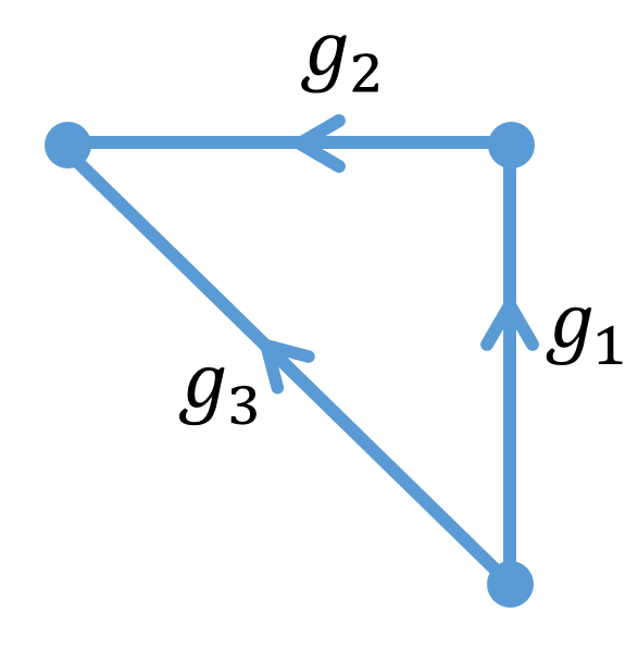
Figure 1: A triangle with this type of orientation is assigned $\alpha_{2}(g_{1},g_{2})$.

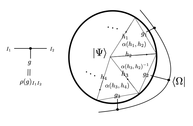
Figure 2: A simple triangulation of a disk and a tensor network representation of the state $\langle\Omega|$.

These triangles satisfy the associativity constraint

$$\frac{\alpha(g_{1},g_{2})\alpha(g_{1}g_{2},g_{3})}{\alpha(g_{1},g_{2}g_{3})\alpha(g_{2},g_{3})}=1.$$ (6)

Using the relation (6), we can convert the boundary circle with $2N$ edges to one with $N$ edges as shown in figure 3. The collection of triangles connecting the two circles of size $2N$ and $N$ has the structure of a tree, and we denote it by $U_{N}(G,\alpha)$.

We identify

$$\exp(z\mathcal{H})\to U(G,\alpha)\equiv\lim_{N\to\infty}U_{N}(G,\alpha)$$ (7)

Eigenstates $\langle\Omega|$ of $U(G,\alpha)$ would define scale invariant partition functions $Z(\Omega,G)$ with global symmetry $G$ through (1). This is illustrated in figure 3.

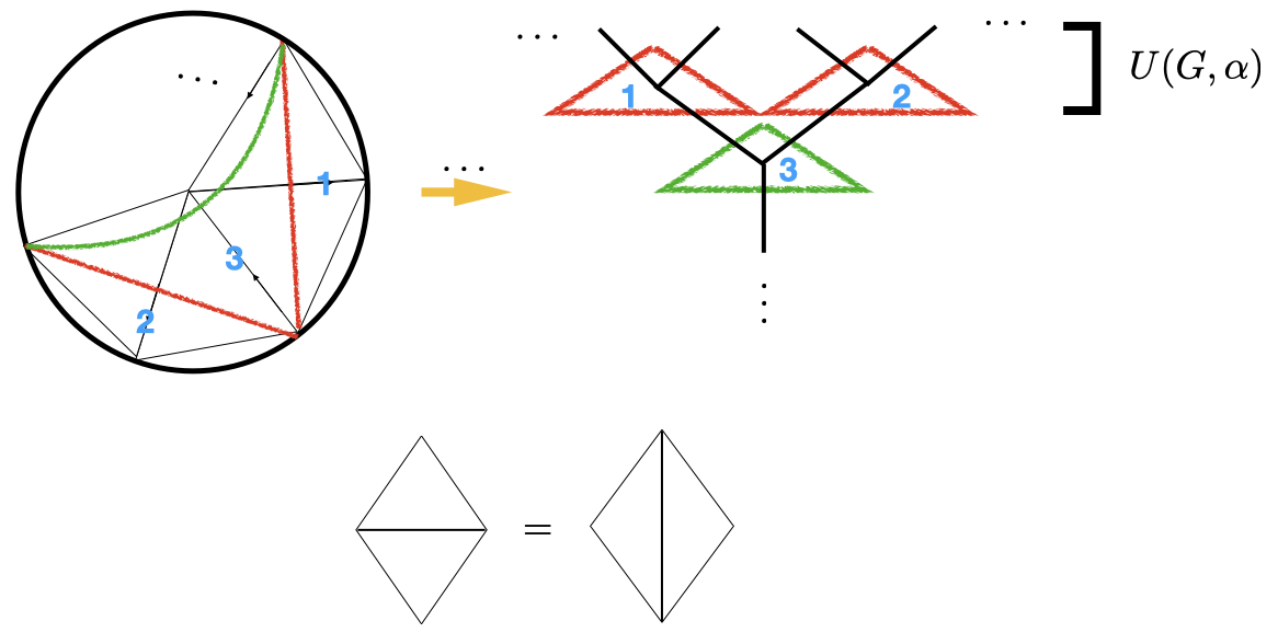
Figure 3: The triangulation of the disk can be converted to a tree-like tensor network by repeated use of the associativity condition (6) which is also illustrated pictorially in the lower half of the figure.

For simplicity, we will focus our discussion on the trivial element of $H^{2}$, such that $\alpha_{2}(g_{1},g_{2})=1$. There is a very simple class of eigenstates. The state is defined on a circle (approaching infinite size). Consider an $\langle\Omega|$ that can be represented by a matrix product state (MPS), meaning that the wave-function of which can be represented as the trace of products of matrices $\rho(g_{i})_{a_{i}b_{i}}$ with $a_{i},b_{i}$ internal auxilliary indices that have dimension $d$. Suppose

$$\langle\Omega|=\sum_{\{g\}}\textrm{tr}(\cdots\rho({g_{i}})\rho({g_{i+1}})\rho({g_{i+2}})\cdots)\langle\cdots g_{i},g_{i+1},g_{i+2}\cdots|,\,\,$$

$$(\rho(g_{1})\rho(g_{2}))_{ac}\equiv\sum_{b}\rho(g_{1})_{ab}\rho(g_{2})_{bc}=\rho(g_{1}g_{2})_{ac},$$ (8)

one can readily check that (8) ensures that $\langle\Omega|$ is in fact an eigenstate of the RG operator $U(G,1)$. Therefore every irreducible representation of $G$ constitutes an eigenstate. One can also show that the most generic form of eigenstates to the RG operator can be decomposed as direct sum of representations of the group $G$, i.e. $\rho(g)=\oplus\rho^{\mu}(g)$, where $\mu$ denotes different representations of the group $G$. The details of the proof are relegated to the appendix.

Therefore $Z(\Omega,G)=\langle\Omega|\Psi\rangle_{G}$ is a summation of finite dimensional traces of products of matrices $T_{I=(a,h),J=(b,k)}(g)=\rho(g)_{a,b}\alpha(h,k)^{\varepsilon}\delta_{g,hk}$. All local correlation functions decay exponentially, proving that $Z(\Omega,G)$ is a topological 1$D$ theory. Physically, we do not expect critical models in 1$D$ and we believe the construction gives a complete construction of 1$D$ models with symmetry $G$.

IV Holographic Networks in 3D

The story can be readily generalised to 3D. Consider a Turaev-Viro type topological theory associated to a fusion category $\mathcal{C}$. To generate the ground state wavefunction on a two-sphere $S_{2}$, we consider the path-integral on a three-ball which is triangulated into tetrahedra. A convenient choice is chosen such that the two dimensional cross section would take the same form as in the 2D case shown in figure 2 above, i.e. the $S_{2}$ is covered by triangles and each corner of the triangle is attached an edge that extends into the ball and ends at the center of the ball. Each edge of the triangulation is assigned an object of $\mathcal{C}$, and each tetrahedron is assigned the value of the 6j symbol that is defined through associativity relation in the fusion of objects of $\mathcal{C}$, as shown in figure 4.

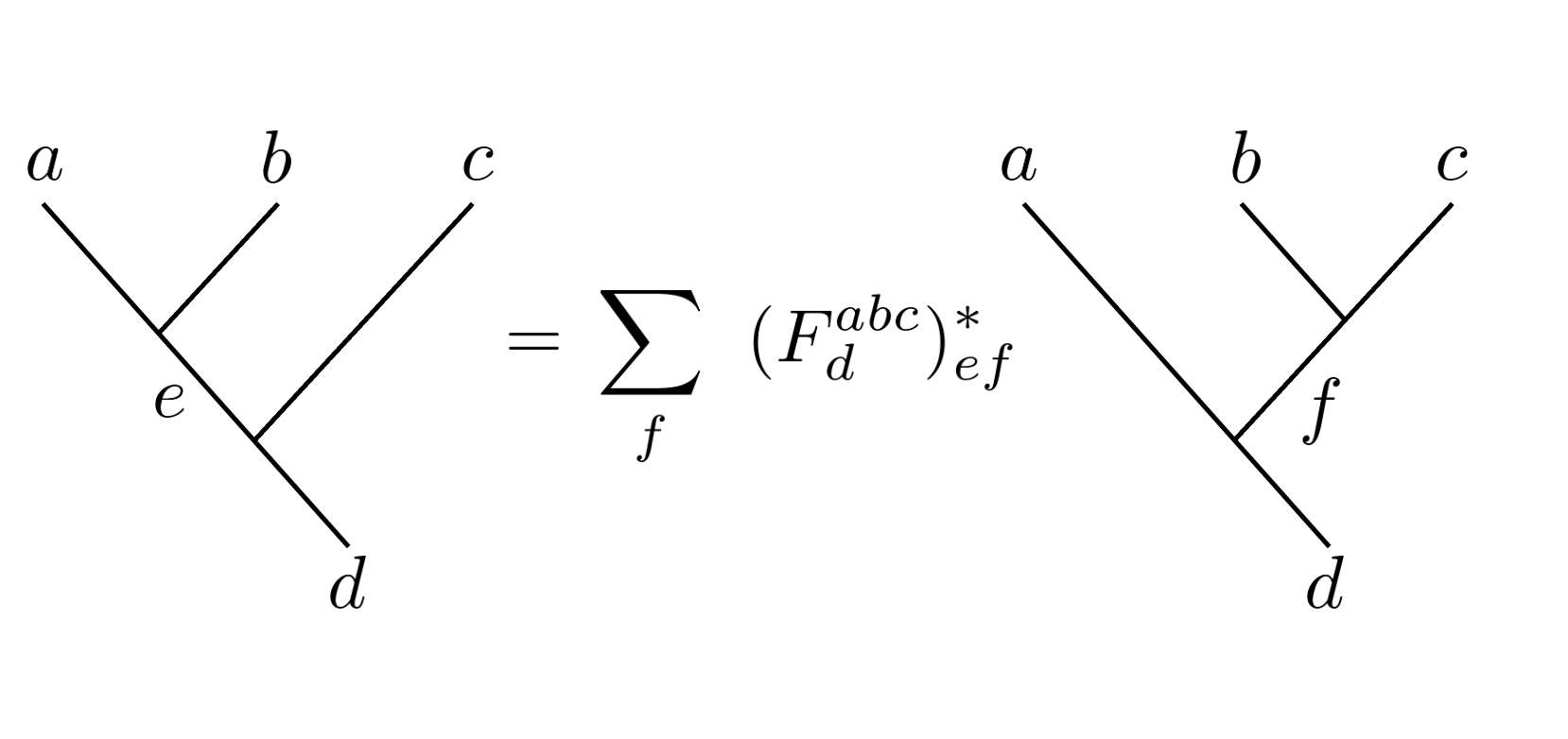
Figure 4: Definition of the 6j symbol.

The objects attached to edges orthogonal to the boundary surface have to be summed, with each edge object $a$ weighted by its quantum dimension $d_{a}$ in the sum. This reproduces the tensor network representation of ground state wave-functions described for example in König et al. (2009); Luo et al. (2017); Williamson et al. (2017); Aasen et al. (2020); Vanhove et al. (2018) and it is represented diagramatically as in figure 5. These triangles are tensors related to the 6j symbols. The relation is illustrated in figure 6, with important relations they satisfy that follow from the pentagon equations.

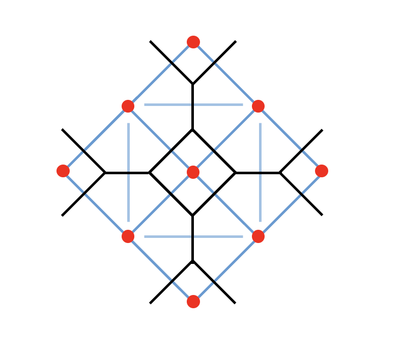
Figure 5: Tensor network representation of the ground state wave-function. The blue lines are “physical sites” of the topological order. The red dots represent edges orthogonal to the $S_{2}$ surface which are weighted by the quantum dimension of the object attached, and summed.

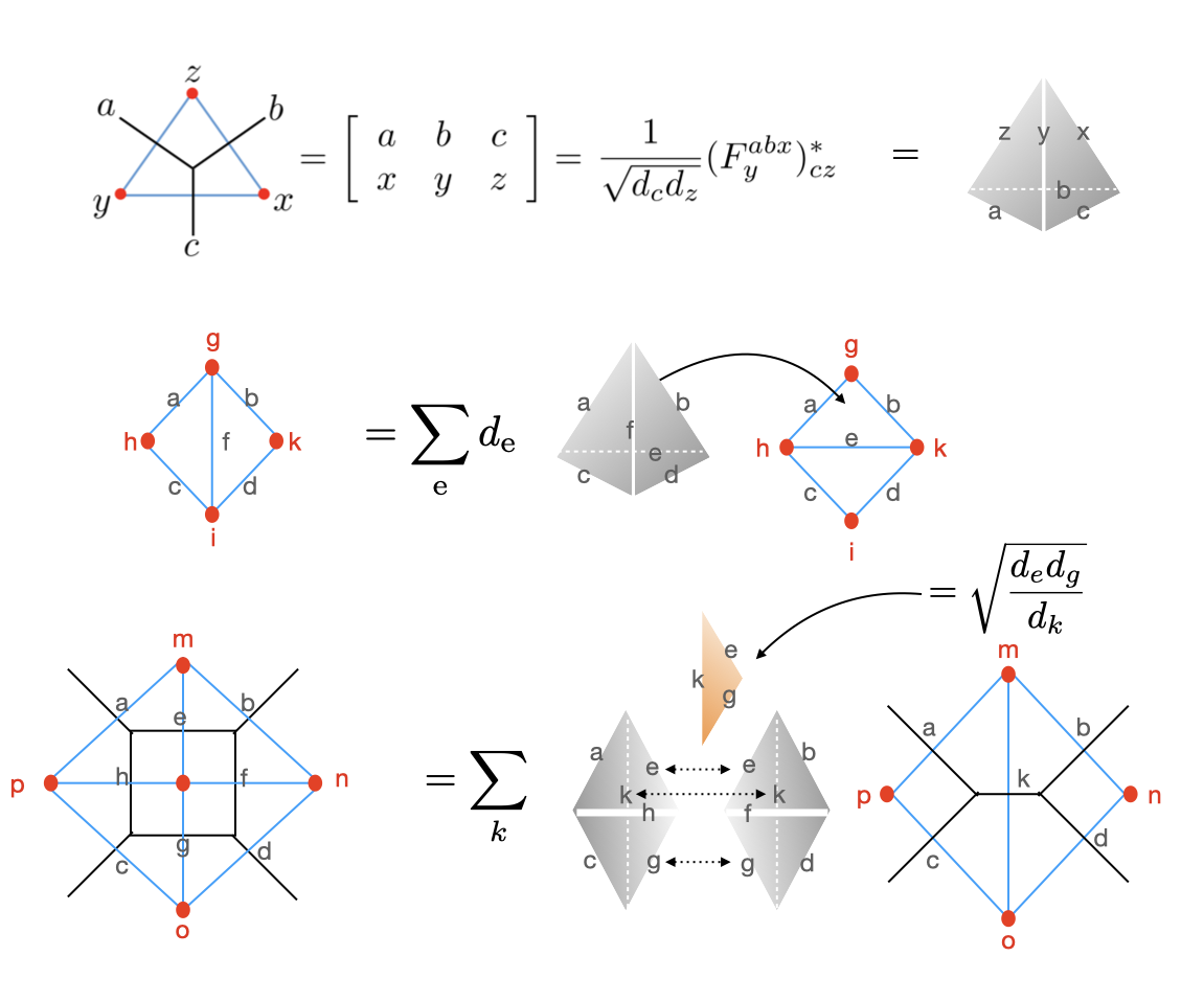
Figure 6: Values of the tensors are given by the 6j symbols. The pentagon equations correspond to stacking an extra tetrahedron onto the surface of other tetrahedra, changing the surface triangulation.

Similar to the 2D case discussed above, the 3D RG operator is constructed by relating two boundaries with different lattice spacings. This can be done by considering a sequence of F-moves and making use of the relations in figure 6. One choice of the blocking sequence is given in figure 7 Vanhove et al. (2018).

Figure 7: Coarse graining using the pentagone relations. The RG operator can be visualised as a collection of tetrahedra. Using the relations in figure 6, we demonstrate the set of factors (grey pair of tetrahedra and a factor of quantum dimensions) needed to convert four triangles into two triangles.

One can express this sequence of blockings as a stack of tetrahedra. This is illustrated in figure 7. The RG operator $U(\mathcal{C})$ in this case, would be the collection of grey tetrahedra and yellow triangles collected in taking the wave-function from the $N$-th RG step to the $N+1$-th step. One can see that $U(\mathcal{C})$ is determined purely by the topological data of the fusion category $\mathcal{C}$. Recursive application of the RG steps would result in a collection of tetrahedra that discretize a Euclidean AdS space. We will return to this point in more detail below.

IV.1 Frobenius Algebra gives Topological Fixed Points

There is a class of eigenstates of $U(\mathcal{C})$. As it is well known, gapped boundaries of 2+1 dimensional topological orders described by say Levin-Wen models are classified by separable Frobenius algebra Fuchs et al. (2002) of the input fusion categories Bullivant et al. (2017); Hu et al. (2018, 2017). It is thus very tempting to look for partition functions of these gapped boundaries making use of knowledge of the Frobenius algebra of the category $\mathcal{C}$. The solution is given by

$$\langle\Omega^{\mu}_{\Lambda}|=\prod_{v}\prod_{l\sim v}\sum_{\{a_{l}\}}\langle a_{l}|T_{\mu}(v),$$ (9)

where $T_{\mu}(v)$ is a projector of every three-edged vertex which will be related to the (co-) product of a Frobenius algebra $A$. The sum over $\{a_{l}\}$ sums over the objects at edge $l$ connected to the vertex $v$, i.e. the partition function is such that we put an extra weight on each vertex. This is illustrated in figure 8.

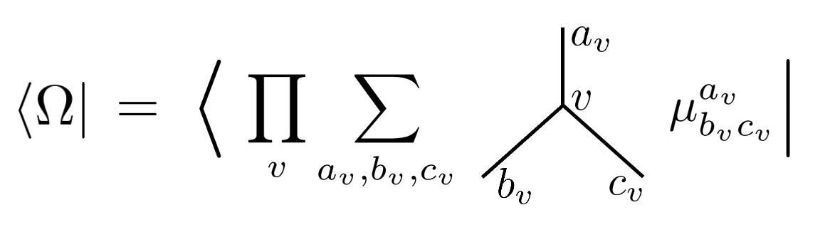
Figure 8: The bra-state $\langle\Omega|$ that follows from a Frobenius algebra is constructed such that every vertex on the 2D surface is weighted by the product coefficient $\mu$ defining the algebra.

The product and co-product of a Frobenius algebra is expressed as in figure 9.

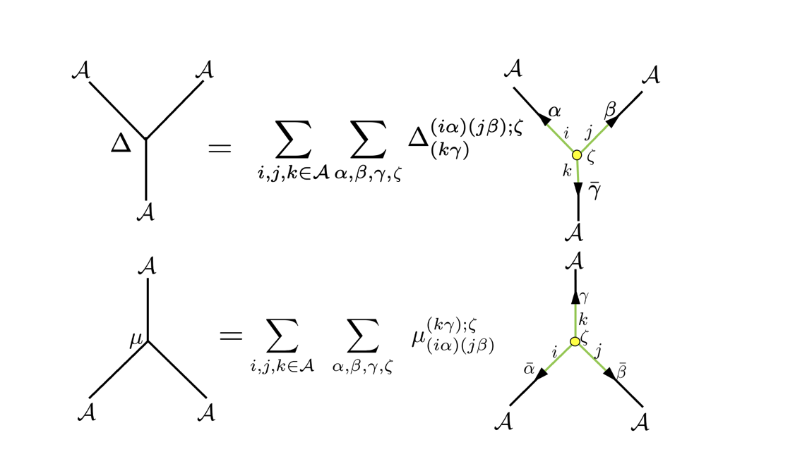
Figure 9: The product $\mu$ and co-product $\Delta$ of a Frobenius algebra expressed in basis form.

For simplicity, where each object is its own dual, it is possible to have the co-product equal to flipping the product, and in such a case, we do not have to distinguish them. In this simple case, we can then require that the value assigned to each triangle is equated with the product, i.e.

$$T_{\mu}=\mu.$$ (10)

In the general case we need to specify the orientation on every edge and then distinguish the product from the co-product.

Since the algebra is Frobenius and separable – as depicted in figure 10, one can readily see that locally, going through the steps depicted in figure 7, $\langle\Omega^{\mu}|$ and $\langle\Omega^{\mu}|U(\mathcal{C})$, look exactly the same – every vertex is still weighted by the same weight characterized by the product map $\mu$ of the Frobenius algebra $A$. Every Frobenius algebra of $\mathcal{C}$ gives a topological 1+1 D TQFT with symmetry characterized by categorical symmetry $\mathcal{Z}(\mathcal{C})$. We note that $\mathcal{Z}(\mathcal{C})$ is spontaneousely broken in each of these TQFT’s. The order parameter in terms of defect operators can be constructed and will be presented in an accompanying paper.

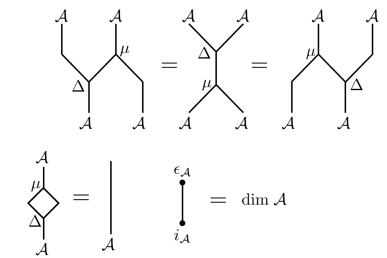
Figure 10: The upper half depicts the associativity of a Frobenius algebra. The lower half depicts the condition of separability.

We note that every separable Frobenius algebra in the input category corresponds to a Lagrangian algebra in the output category associated to the topological order. Each Lagrangian algebra describes a spatial gapped boundary condition of the topological order which is physically prescribing a collection of anyons condensing at the boundary. We note however, that different Frobenius algebra of the input category might be mapped to the same or isomorphic Lagrangian algebra in the output category which is often considered as physically equivalent in the literature Hu et al. (2017). As we are going to see below however, they lead to different 2D TQFT through the strange correlator, and there are CFT’s describing phase transitions between them.

IV.2 CFTs from phase transitions between fixed points

The most interesting question is to construct partition functions of critical points. A critical point is reached when non-commuting topological symmetries are preserved at the same time Levin (2020); Ji and Wen (2020); Chatterjee and Wen (2022b, a). Since $Z(\mathcal{C})$ is supposedly a local partition function, we expect that $\langle\Omega|$ should admit a PEPS tensor network construction. Inspired by the form of the topological solution above where $\langle\Omega|$ is essentially a direct product of states defined on each triangle, we construct an ansatz where each tensor covers a triangle with 6 legs i.e. $T^{a_{1}a_{2}a_{3}}_{I_{1}I_{2}I_{3}}$, i.e. each edge of the triangle carries a pair of indices, where $a_{i}\in\mathcal{C}$ and $I_{i}$ are auxilliary indices with bond dimension $\eta$. In principle one could constrain the form of $T^{a_{1}a_{2}a_{3}}_{I_{1}I_{2}I_{3}}$ by imposing that these open topological string operators die off at most with a power-law as a function of distance between the end points. In practice, checking for power law decay is highly non-trivial – it suggests that $\eta$ should scale with system size and approach infinity for an infinite system. We will adopt a different approach to extract critical point data. Consider a single RG step $\langle\Omega(T)|U(\mathcal{C})$. As demonstrated in figure 7, four triangles are mapped to two triangles with entangled boundary conditions. By applying for example, singular value decomposition (SVD) and keeping a fixed bond dimension for auxiliary indices $I_{i}$, one can rewrite the products of four $T$’s as a contraction of two new tensors $\tilde{T}$, as shown in the figure 11. For finite $\eta$, the critical point is unstable and the sequence of $T$’s obtained from the RG process would eventually flow to one of the topological fixed points. By appropriate parametrisation of $T$, we would be able to find out critical points where the RG process begins to be confused about which topological fixed point to go to. For every fixed $\eta$ it is thus possible to obtain $T$’s that are best approximating the critical state.

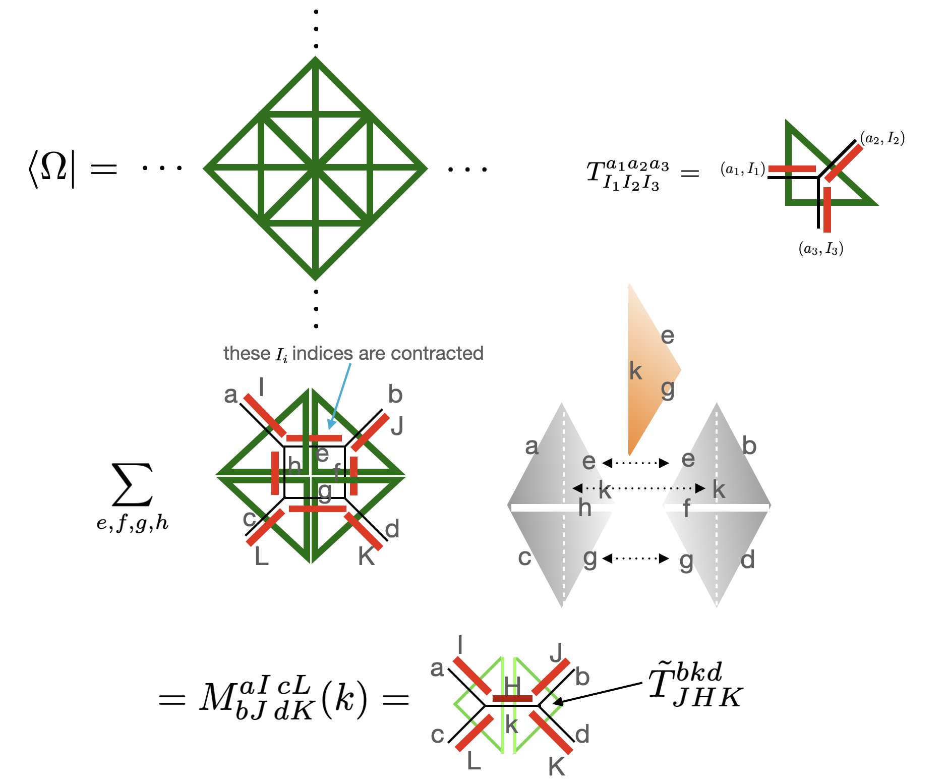
Figure 11: The top figure illustrates the PEP construction of the boundary state $\langle\Omega|$. The indices lives on the edges of the triangles (or edges on the dual graph). Each edge carries a pair of indices, $a_{i}\in\mathcal{C}$ and $I_{i}$ are auxiliary indices with bond dimension $\eta$. In the bottom figure, we break down the tensor $M(k)$ into the product of two $\tilde{T}$’s (light green triangles). This breaking down can be achieved by SVD. The new auxiliary index $H$ (colored dark red) is generically of dimension $\eta^{2}$, but we would cut it off down to dimension $\eta$.

IV.3 Some Explicit Examples

IV.3.1 The A-series minimal CFTs

We can demonstrate in a class of examples constructed from the fusion category formed by representations of the quantum group $SU(2)_{k}$. At level $k$, there are $k+1$ objects $j=0,1/2,\cdots,k/2$. They satisfy the fusion rule

$$j_{1}\otimes j_{2}=|j_{1}-j_{2}|\oplus(|j_{1}-j_{2}|+1)\oplus\cdots\oplus\textrm{min}\{j_{1}+j_{2},k-j_{1}-j_{2}\}.$$ (11)

In particular, one sees that $1/2\otimes 1/2=0\oplus 1$. Consider a family of boundary state $\langle\Omega|$ taking the form

$$\langle\Omega|=\sum_{\{a\}}\langle\{a\}|\prod_{\Delta_{2}}T_{\Delta_{2}},$$ (12)

where the summation is over all the configurations, and each triangle on the boundary contributes $T_{\Delta_{2}}$. The boundary condition is such that each $T_{\Delta_{2}}$ attached to a triangle $\Delta_{2}$ is given by the three index tensor $T^{a_{1}a_{2}a_{3}}$ chosen to be

$$T^{a_{1}a_{2}a_{3}}=\left\{\begin{aligned} 1&,&(a_{1}=a_{3}=\frac{1}{2},a_{2}=0),\\ r&,&(a_{1}=a_{3}=\frac{1}{2},a_{2}=1),\\ 0&,&(\textrm{Otherwise}).\end{aligned}\right.$$ (13)

This is depicted in figure 12. Comparing with the top of figure 11, this corresponds to the case where the extra index $I_{i}$ attached to an edge is trivial ( i.e. bond dimension 1).

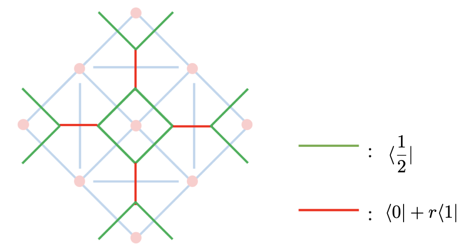
Figure 12: A family of boundary conditions for $SU(2)_{k}$ models with one parameter $r$. At $k=2$ one recovers the 2D Ising model at temperature $e^{-2\beta}=r$.

For every $k$, there is a critical coupling $r=r_{c}(k)$ which is known to recover in the thermodynamic limit, the A-series minimal CFT. We would like to recover the critical coupling using the method we discussed above i.e. allowing the tensor $T$ to flow under repeated use of the RG operator. Starting with this boundary state, we carry out the RG process described in figure 11 with bond dimension for the auxiliary indices kept, as a very crude approximation, at $\eta=1$. And we find that for small $r$, the boundary state flows to a fixed point where $T^{a_{1}a_{2}a_{3}}$ only has one non-vanishing component $T^{000}$, i.e. all the boundary legs are projected to the identity element, denoted 0 here. This is of course a separable Frobenius algebra for any fusion category. We call that $\mathcal{A}_{0}$. For bigger $r$, the boundary state flows to a fixed point where $T^{a_{1}a_{2}a_{3}}$ has the following non-vanishing components $T^{000}=T^{110}=T^{101}=T^{011}$ and $T^{111}$ (this component appears when $k>2$). The ratio $T^{000}/T^{111}$ is a function of $k$. When $k=3$, $T^{000}/T^{111}=1.43463$. When $k=4$, $T^{000}/T^{111}=1.18921$. We note that this coincides precisely with a family of separable Frobenius algebra of $SU(2)_{k}$ category. The objects in the algebra is given by $\mathcal{A}_{1}=\{0,1\}$, and the ratio of the product of the algebra $T^{000}_{\mu(k)}/T^{111}_{\mu(k)}$ for arbitrary $k>2$ is given by

$$\frac{T^{000}_{\mu(k)}}{T^{111}_{\mu(k)}}=\frac{\sqrt[4]{2\cos\left(\frac{2\pi}{k+2}\right)+1}}{\sqrt{2\cos\left(\frac{2\pi}{k+2}\right)}}.$$ (14)

The separable Frobenius algebra is generated by the RG algorithm!

The critical coupling $r_{c}(k)$ determining the phase transitions between the two fixed points characterized by the algebra $\mathcal{A}_{0}$ and $\mathcal{A}_{1}$ are determined numerically. We compare our numerical results with the analytical one in figure 13. At the critical point, Kramers-Wannar duality is preserved in this series of models and the critical couplings can thus be readily obtained as benchmarks. The numerical results recover the analytical result to about 1 significant figure. This is quite remarkable given that we adopted such a brutal truncation with auxiliary bond dimension 1. The method can be readily adopted with larger bond dimensions and is currently work underway.

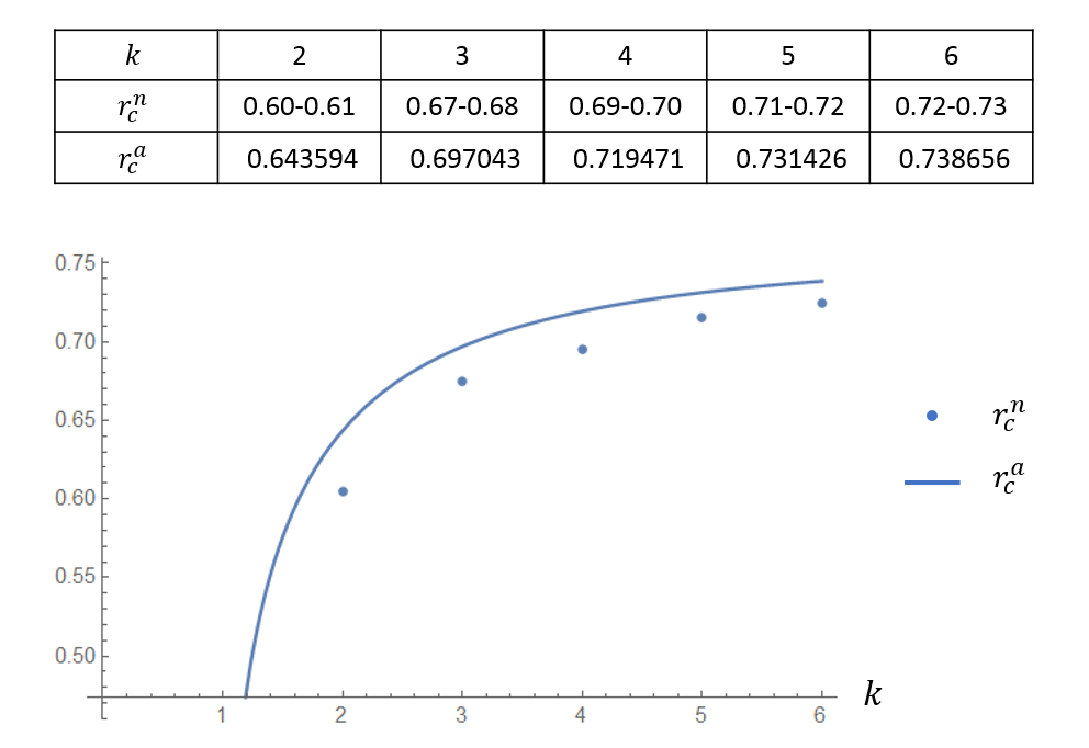
Figure 13: Here $r^{n}_{c}$ is the numerical result for the phase transition point, and $r^{a}_{c}$ is the analytical result which is given by $r^{a}_{c}=\sqrt{\frac{\sqrt{2\cos\left(\frac{2\pi}{k+2}\right)+1}}{2\cos\left(\frac{\pi}{k+2}\right)+1}}.$

Here we would like to note that the CFT is a phase transition point between two topological fixed points of the RG operator described by two Frobenius algebras in the input category $\mathcal{C}$. For example in the case of $k=2$, these two algebras $\mathcal{A}_{0}$ and $\mathcal{A}_{1}$ correspond to the same set of anyon condensations in the output category (the topological order the lattice model describes) Hu et al. (2017). Specifically, the output category is a doubled Ising topological order where there are 9 topological sectors that can be labeled by the pair $(j_{1},\bar{j}_{2})$, where $j_{1,2}\in\{0,1/2,1\}$. Here, both Frobenius algebra in the input category, $\mathcal{A}_{0}$ and $\mathcal{A}_{1}$, correspond to the same condensable Lagrangian algebra in the output category, namely $(0,\bar{0})\oplus(1/2,\bar{1/2})\oplus(1,\bar{1})$. However, we can see here that physically they lead to different 2D topological fixed points and a physical phase transition between them is exactly the 2D Ising CFT connects them, which is a point observed also in Ji and Wen (2020). The two topological fixed points are interpreted as the electric and magnetic condensate respectively if we do not include the Kramers-Wannier duality in the categorical symmetry, leaving the bulk reduced to the 2+1 D toric code. (The doubled Ising bulk and the toric code are related by anyon condensation too – condensing $(0,\bar{0})\oplus(1,\bar{1})$Bais and Slingerland (2009).) In terms of categorical symmetry, the toric code version breaks spontaneousely the Kramers-Wannier duality that is kept explicit in the doubled Ising bulk. One should thus take extra care when seeking phase transition points between topological fixed points. The condensable algebra of the output category might undercount the number of fixed points, unless we take into account isomorphic algebras with the same collection of condensing anyons as physically distinct.

IV.3.2 A curious example

When $k=4$, we also consider the case that $T^{a_{1}a_{2}a_{3}}$ is given by

$$T^{a_{1}a_{2}a_{3}}=\left\{\begin{aligned} 1&,&(a_{1}=a_{3}=1,a_{2}=0),\\ r_{1}&,&(a_{1}=a_{3}=1,a_{2}=1),\\ r_{2}&,&(a_{1}=a_{3}=1,a_{2}=2),\\ 0&,&(\textrm{Otherwise}).\end{aligned}\right.$$ (15)

We carry out the RG process described in figure 11 with bond dimension $\eta=1$, and find that the boundary state can flow to 3 different fixed points when we change $r_{1},r_{2}$. In the type I fixed point, $T^{a_{1}a_{2}a_{3}}$ only has one non-vanishing component $T^{000}$, i.e. all the boundary legs are projected to 0. In the type II fixed point, $T^{a_{1}a_{2}a_{3}}$ has following non-vanishing components $T^{000}=T^{022}=T^{202}=T^{220}$. In the type III fixed point, $T^{a_{1}a_{2}a_{3}}$ has following non-vanishing components $T^{000}=T^{011}=T^{101}=T^{110}=T^{022}=T^{202}=T^{220}=T^{112}=T^{121}=T^{211}$ (the component $T^{111}$ is allowed by the fusion rules but is 0). And the phase diagram is shown in figure 14. The triple point is around $(r_{1},r_{2})=(0.7,0.6)$.

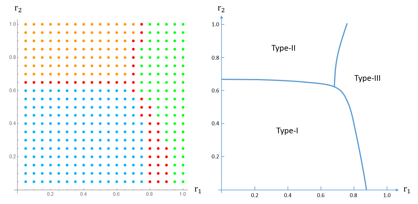
Figure 14: The left hand side is our numerical result. The blue/orange/green dots correspond to type I/II/III fixed points. The red dots are those we can’t tell its fixed point type within 10 RG steps. According to the numerical result, we can obtain a phase diagram shown on the right hand side.

We are currently working on figuring if this tricritical point corresponds to a (known) CFT.

V Holographic Networks and RG operator in 4d

One can construct 3D partition functions from strange correlators with ground state wave-functions of 4D TQFT. Generically, the topological input data of the 4D TQFT involves a 2-fusion category Lan and Wen (2019); Johnson-Freyd (2022); Douglas and Reutter (2018); Johnson and Yau (2020). The geometrical building block of 4D TQFT is a 4-simplex. One assigns objects of the 2-category to the edges, fusion 1-morphism to each surface and 2-morphism to the 3-sub-simplex. Here, we would focus on the 4D Dijkgraaf-Witten model. In that case, each model is characterized by a group $G$, and an element of $H^{4}(G,U(1))$. Group elements of $G$ play the role of objects and are again assigned to the edges, and the 4-simplex is a function $\alpha(\{g_{i}\})\in H^{4}(G,U(1))$ of the 10 edges. Fusion between objects is reduced to the group product.

The 3+1 D TQFT ground state $|\Psi\rangle$ admits tensor network representations that are natural generalization of the 3D case. The ground state wave-function can be obtained from a path-integral of a 4-ball with a 3-sphere boundary. The path-integral is obtained by considering a triangulation of boundary 3-space into 3-simplices. Each of these 3-simplices belongs to a 4-simplex. They all share an index in the center of the 4-ball, which is a higher dimensional generalization of figure 2. As a tensor network, the building block can be written as a tetrahedron with indices both on the edges and on the vertices. The 4D ground state wave-function defined on a 3D surface is obtained by putting these tetrahedra together filling the 3D space, and summing over the indices on the shared vertices between tetrahedra. A version of this tensor network is discussed in Delcamp and Schuch (2021) for the 3+1 D toric code model. Here we follow a direct generalization of the picture in the 2+1 D and 1+1 D case with a notation adapting to that in Aasen et al. (2020). The discussion should apply quite generally to any 3+1 D topological models based on 2-fusion categories.

For concreteness, we pick a specific triangulation of the 3D surface. First fill the 3D space with cubes. Each vertex (colored green in figure 15) is shared between 8 cubes and the group element attached to it would be summed over. Then each cube is divided into 6 tetrahedra, as shown in figure 15. In this triangulation of the cube, two vertices (1 and 7) play a special role.

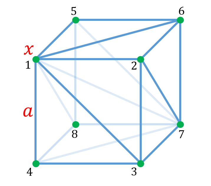
Figure 15: Each cube is divided into 6 tetrahedra. They are $1237$, $1267$, $1567$, $1587$, $1487$, $1437$. We remark that they are one to one correspondence to the paths from vertex 1 to vertex 7. Vertex 1 and vertex 7 are diagonal on the cube, and they determine the triangulation of the cube. Green dots represent the bulk edges. The bulk edges are labeled by $x$. The boundary edges are labeled by $a$.

A complete specification of the triangulation therefore involves marking the cubic lattice vertices that play the special role used in the above triangulation which are marked red in figure 16. Including this structure, the smallest self-repeating unit is a $2\times 2\times 2$ collection of cubes.

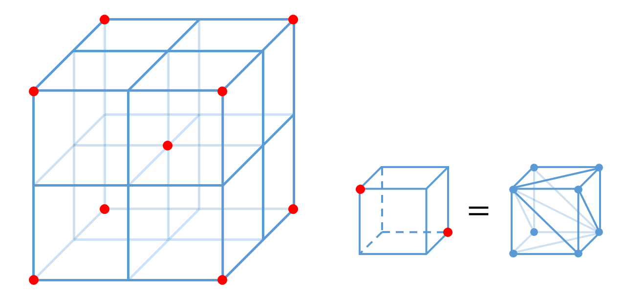
Figure 16: Each $2\times 2\times 2$ cube contains 8 small cubes. Each small cube has two red dots on its diagonal vertices. And the triangulation of small cube is determined by these two red dots. Previously we use green dots to represent bulk edges. Here the blue dots are just the vertices of the small cubes.

The RG operator we will construct below involves mapping the $2\times 2\times 2$ cube into 1 cube as shown in figure 17.

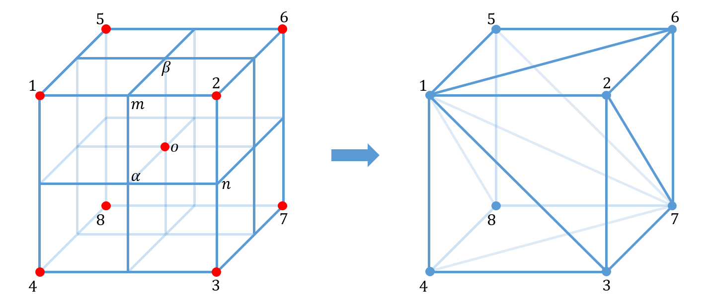
Figure 17: Coarse grain the $2\times 2\times 2$ cube into $1\times 1\times 1$ cube.

This is achieved in three steps. But to that end, we need to use a generalization of the pentagon relation leading to figure 6. In the case of the Dijkgraaf-Witten models, this is just the 4-cocycle relation Dijkgraaf and Witten (1990), which is explained in the beginning of Appendix B.

Using the 4-cocycle relation, we can thus map two tetrahedra into one, as illustrated in figure 18. Through this map, one vertex is eliminated as a result. We will thus in the following discuss the RG process as a sequence of steps that eliminate designated vertices through repeated use of this relation in figure 18, keeping the collection of 4-cocycles, or often called 10-j symbols accumulating implicitly.

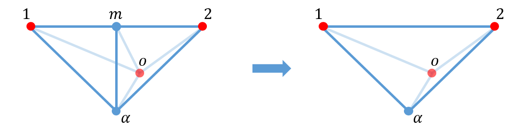
Figure 18: Combine $1m\alpha o$ and $2m\alpha o$ to get a bigger tetrahedron $12\alpha o$.

The first step is to eliminate the vertices $m,n,\dots$ in the middle of the edges of the $2\times 2\times 2$ cube and obtain the edges $12,23,\dots$ of the target $1\times 1\times 1$ cube. Let’s consider the vertex $m$ as an example. It is shared by 4 tetrahedra: $1m\alpha o,1m\beta o,2m\alpha o,2m\beta o$. Now we combine $1m\alpha o$ and $2m\alpha o$ to get a bigger tetrahedron $12\alpha o$ as shown in figure 18. Similarly combining $1m\beta o$ and $2m\beta o$ will give us tetrahedron $12\beta o$. And then the vertex $m$ disappears and the edge $12$ is obtained. In the 4D perspective, we have a 4-simplex $12m\alpha o$ whose boundary consists of 5 tetrahedra: $1m\alpha o,2m\alpha o,12\alpha o,12mo,12m\alpha$. One can note that $1m\alpha o,2m\alpha o,12\alpha o$ appear in the combining procedure. While $12mo$ is shared by a neighboring 4-simplex $12m\beta o$, and $12m\alpha$ is similarly shared by another neighboring 4-simplex. So the combining procedure is actually achieved by inserting these 4-simplices. They form a 4D body which has two boundaries. One boundary consists of small tetrahedra $1m\alpha o,1m\beta o,2m\alpha o,2m\beta o$, and the other boundary consists of bigger tetrahedra $12\alpha o,12\beta o$.

Notice that the vertex $m$ is shared by four $2\times 2\times 2$ cubes. In the above we only consider one of them. The whole picture is given by figure 19, where $o_{1},o_{2},o_{3}$ are the centers of other three $2\times 2\times 2$ cubes. We have eight 4-simplices $12m\alpha o,12m\beta o$, $12m\beta o_{1},12m\gamma o_{1}$, $12m\gamma o_{2},12m\delta o_{2}$, $12m\delta o_{3},12m\alpha o_{3}$. The adjacent simplices share the same tetrahedron: for example, $12m\alpha o,12m\beta o$ share the tetrahedron $12mo$. Finally these 4-simplices form a 4D body which has two boundaries. One boundary consists of 16 small tetrahedra $1m\alpha o,1m\beta o,1m\beta o_{1},\dots,2m\alpha o,2m\beta o,2m\beta o_{1}\dots$, and the other boundary consists of 8 bigger tetrahedra $12\alpha o,12\beta o,12\beta o_{1},\dots$. The 4D body is a map between these two boundaries. After applying this type of maps, we remove the vertices $m,n,\dots$ in the middle of the edges of the $2\times 2\times 2$ cube, and obtain edges $12,23,\dots$ of the target $1\times 1\times 1$ cube.

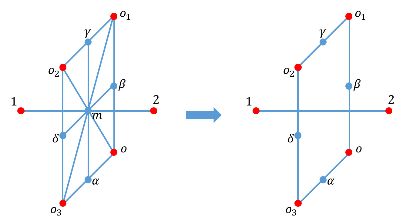
Figure 19: The first step is to eliminate the vertices like $m$ and to obtain edges like $12$. To avoid clutter, we omit the edges connecting $1,2$ with $\alpha,\beta,\gamma,\delta,o,o_{1},o_{2},o_{3}$. On the left hand side, there is a vertex $m$, and there are 16 small tetrahedron $1m\alpha o,1m\beta o,1m\beta o_{1},\dots,2m\alpha o,2m\beta o,2m\beta o_{1}\dots$. On the right hand side, there is no $m$, and there are 8 bigger tetrahedron $12\alpha o,12\beta o,12\beta o_{1},\dots$. They are on the two boundaries of a 4D body which consists of eight 4-simplices $12m\alpha o$, $12m\beta o$, $12m\beta o_{1}$, $12m\gamma o_{1}$, $12m\gamma o_{2}$, $12m\delta o_{2}$, $12m\delta o_{3}$, $12m\alpha o_{3}$.

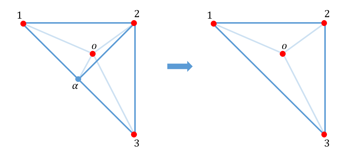
Figure 20: Combine $12\alpha o$ and $23\alpha o$ to get a bigger tetrahedron $123o$.

The second step is to eliminate the vertices $\alpha,\beta,\dots$ in the center of faces of the $2\times 2\times 2$ cube and obtain the edges $13,16,\dots$ in the target $1\times 1\times 1$ cube. Let’s consider the vertex $\alpha$ as an example. After the first step, it is shared by 4 tetrahedra: $12\alpha o,23\alpha o,34\alpha o,41\alpha o$. Now we combine $12\alpha o$ and $23\alpha o$ to get a bigger tetrahedron $123o$ as shown in figure 20. Similarly combining $34\alpha o$ and $41\alpha o$ will give us tetrahedron $341o$. And then the vertex $\alpha$ disappears, and the edge $13$ is obtained. The vertex $\alpha$ is actually shared by two $2\times 2\times 2$ cubes. The whole picture is given by figure 21, where $o_{3}$ is the center of the other $2\times 2\times 2$ cube. We have four 4-simplices $123\alpha o,123\alpha o_{3},341\alpha o_{3},341\alpha o$. And these 4-simplices form a 4D body which has two boundaries. One boundary consists of 8 tetrahedra $12\alpha o,23\alpha o,34\alpha o,41\alpha o,12\alpha o_{3},23\alpha o_{3},34\alpha o_{3},41\alpha o_{3}$, and the other boundary consists of 4 tetrahedra $123o,341o,123o_{3},341o_{3}$. The 4D body is a map between these two boundaries. After applying this type of maps properly, we remove the vertices $\alpha,\beta,\dots$ in the center of faces of the $2\times 2\times 2$ cube, and obtain edges $13,16,18,72,74,75$ in the target $1\times 1\times 1$ cube.

Figure 21: The second step is to eliminate the vertices like $\alpha$. Here we choose to connect vertices $1,3$ since in the target coarse grained cubic there is a $13$ edge as shown in figure 17. On the left hand side, there is a vertex $\alpha$, and there are 8 tetrahedra $12\alpha o,23\alpha o,34\alpha o,41\alpha o,12\alpha o_{3},23\alpha o_{3},34\alpha o_{3},41\alpha o_{3}$. On the right hand side, there is no $\alpha$, and there are 4 tetrahedra $123o,341o,123o_{3},341o_{3}$. They are on the two boundaries of a 4D body which consists of four 4-simplices $123\alpha o,123\alpha o_{3},341\alpha o_{3},341\alpha o$.

The third step is to eliminate the vertex $o$ in the center of the $2\times 2\times 2$ cube and obtain the edge $17$. After the second step, the vertex $o$ is shared by 12 tetrahedra $123o,143o,237o,267o,126o,156o$, $148o,158o,487o,437o,567o,587o$ as shown on the left hand side of figure 22. Now we combine $123o$ and $237o$ to get a bigger tetrahedron $1237$. Similarly the tetrahedra $1267,1567,1587,1487,1437$ in the target cube can be obtained by combining two of these 12 tetrahedra. And then the vertex $o$ disappears, and the edge $17$ is obtained. The whole picture is shown by figure 22. We have six 4-simplices $1237o,1267o,1567o,1587o,1487o,1437o$. And these 4-simplices form a 4D body which has two boundaries. One boundary consists of 12 tetrahedra $123o,143o$, $237o,267o$, $126o,156o$, $148o,158o$, $487o,437o$, $567o,587o$, and the other boundary consists of 6 tetrahedra $1237$, $1267$, $1567$, $1587$, $1487$, $1437$. The 4D body is a map between these two boundaries. After applying this map, we remove the vertex $o$ in the center of the $2\times 2\times 2$ cube, and obtain the edge $17$ in the target $1\times 1\times 1$ cube.

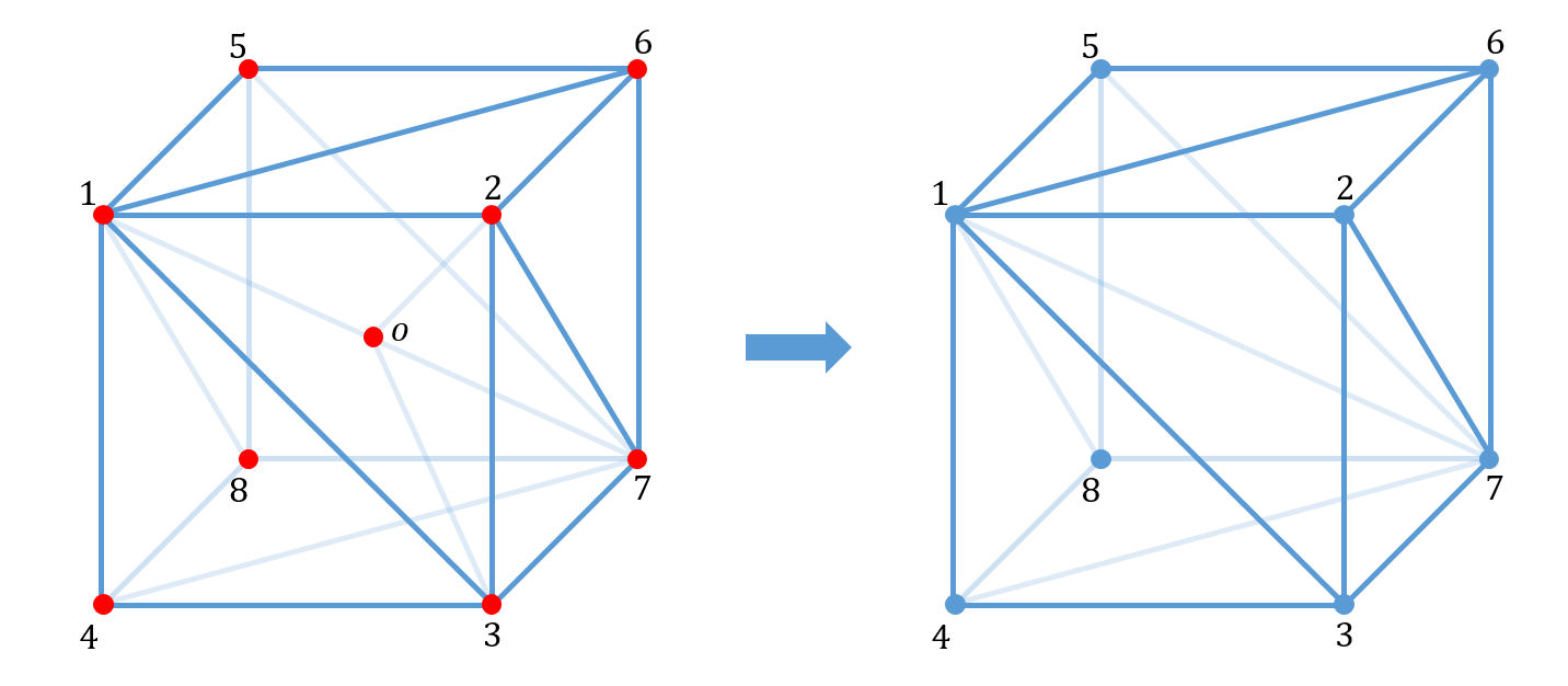
Figure 22: The third step is to eliminate the vertex $o$ and to obtain the edge $17$. To avoid clutter, we only show some of the edges connecting $o$ with $1,2,3,4,5,6,7,8$. On the left hand side, there is a vertex $o$, and there are 12 tetrahedra $123o,143o$, $237o,267o$, $126o,156o$, $148o,158o$, $487o,437o$, $567o,587o$. On the right hand side, there is no $o$, and there are 6 tetrahedra $1237$, $1267$, $1567$, $1587$, $1487$, $1437$. They are on the two boundaries of a 4D body which consists of six 4-simplices $1237o,1267o,1567o,1587o,1487o,1437o$. Combining $123o$ and $237o$ to get the tetrahedron $1237$ can be read off from this figure.

After the 3 steps described above, we coarse grain the $2\times 2\times 2$ cubes into exactly 1 cube. Eight such cubes can be arranged into a structure of $2\times 2\times 2$ cubes shown in figure 16 . This is the same as the original structure. And these 3 steps form one RG step.

V.1 Higher Frobenius Algebra gives Topological Fixed Points

Like in the case of RG operators from 3D topological theories where topological fixed points are given by Frobenius algebra, the RG operator constructed from 4D topological order presented above also admits fixed points based on higher dimensional generalization of Frobenius algebra. In the case where the bulk is given by DW theory, the Frobenius algebra characterizing topological boundary conditions has been studied Wang et al. (2018); Zhao et al. (2022). Together with a higher generalization of “separability” that we will discuss below, we obtain fixed points of the 4D topological RG operators.

These topological eigenstates are constructed as follows. Previously in figure 8, the ground state wave-function is constructed by assigning a weight to every triangle on the 2 dimensional surface, and these weights define the product of a Frobenius algebra of the input fusion category. In the current case the wave-function is defined in 3 dimensions, and we instead assign a value $\tilde{\beta}(g,h,k)$ to every tetrahedron, which has three independent edge degrees of freedom after taking into account of the face constraints. The wavefunction is thus given by

$$\langle\Omega(\tilde{\beta})|=\sum_{\{g_{l}\}}\prod_{\Delta}\tilde{\beta}(g_{\Delta_{1}},g_{\Delta_{2}},g_{\Delta_{3}})\langle\{g_{l}\}|,$$ (16)

where $\Delta$ runs over all tetrahedra that triangulate the three dimensional space, $\Delta_{1,2,3}$ denote 3 independent edges of a tetrahedron, and $\{g_{l}\}$ denotes the collection of all edge degrees of freedom.

Frobenius algebras associated to 4D DW models have been studied and each is associated with a 2+1 D topological boundary condition Wang et al. (2018); Zhao et al. (2022). The data that goes into defining a higher Frobenius algebra involves the collection of objects $\mathcal{A}$ in the fusion category, which is a subgroup in the current case. We also need to define the product between objects and also the associativity map Wang et al. (2018); Zhao et al. (2022). The data can be encapsulated in assigning a function $\beta(g_{\Delta_{1}},g_{\Delta_{2}},g_{\Delta_{3}})$ to every tetrahedron. This function satisfies the following relation:

$$\frac{\alpha(h_{0},h_{1},h_{2},h_{3})\beta(h_{0},h_{1}.h_{2},h_{3})\beta(h_{0},h_{1},h_{2})\beta(h_{1},h_{2},h_{3})}{\beta(h_{0},h_{1},h_{2}.h_{3})\beta(h_{0}.h_{1},h_{2},h_{3})}$$

$$=1,$$ (17)

where $\alpha$ is the 4-cocycle in $H^{4}(G,U(1))$ that defines the DW theory. The 4-cocycle $\alpha$ involved above is precisely a 4-simplex, that maps between two sets of tetrahedra. The geometric meaning of (V.1) is demonstrated in figure 23.

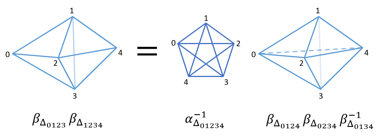
Figure 23: There are 2 tetrahedra on the left and 3 tetrahedra on the right corresponding to two different triangulations of the boundary. We have $\beta_{\Delta_{0123}}\beta_{\Delta_{1234}}=\alpha_{\Delta_{01234}}^{-1}\beta_{\Delta_{0124}}\beta_{\Delta_{0234}}\beta_{\Delta_{0134}}^{-1}$. The powers of $-1$ are related to the orientations.

The above condition is the higher dimensional analogue of associativity in a higher Frobenius algebra. (The condition at least for Frobenius algebra in a n-dimensional DW theory is reviewed in the appendix.) In addition to that, we require also a condition analogous to the separability in 2+1 dimensional topological order. This condition is illustrated in figure 24.

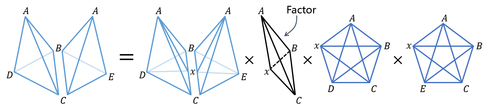
Figure 24: The blue tetraheron corresponds to the boundary factors $\beta$. The pair of 4-simplices on the right hand side corresponds to the 4-cocycles of the DW theory. The black tetrahedron referred to as a “factor” is the analogue of a bubble that is contracted. The equality is based on absorbing this black tetrahedron and is thus the analogue of separability in 2+1 dimensional topological order. In the current model however the factor is equal to unity.

.

We note that algebra satisfying (V.1) were considered as spatial boundary conditions of the DW models. Here however, when inserted into (16) and then subsequently constructing the strange correlator $\langle\Omega(\beta)|\Psi\rangle$, each such boundary condition $\beta$ is in 1-1 correspondence with an SPT phase in 2+1 D with global symmetry $G$ when the 4-cocycle $\alpha$ is trivial. This generalizes explicit realization of the holographic relation discussed in the previous sections to the case of 3+1 D topological order / 2+1 D gapped theories with symmetries $G$. The construction should work for a generic categorical symmetry describable by 3+1 D lattice models with a 2-fusion category as input category.

V.2 CFTs from phase transitions between fixed points – 2+1 D Ising as an example

Much like the situation of constructing partition functions in 2D from 3D topological order, we can obtain 3D CFT partition functions by looking for phase transitions between the topological fixed points to the RG operator we have defined above.

A judicious parametrization of the boundary state $\langle\Omega|$ is important towards obtaining a critical point numerically.

We will work with an explicit example of the 3+1 D toric code Hamma et al. (2005), corresponding to the $G=\mathbb{Z}_{2}$ DW theory in 4D. In this case $H^{4}(\mathbb{Z}_{2},U(1))$ is trivial and the 4-cocycle satisfies $\alpha=1$ when the edge group elements $h_{i}\in\mathbb{Z}_{2}$ satisfy $h_{1}h_{2}=h_{3}$ wherever the edges concerned form a closed triangle, and zero otherwise.

First, we note that the partition function of the well-known 2+1 D lattice Ising model is recovered as a strange correlator between a direct product state $\langle\Omega|$ and the 3+1D toric code ground state wavefunction $|\Psi\rangle$. We will take the triangulation as shown in figure 16 and make use of the tensor network construction described there to recover its wave-function. The boundary state is chosen as follows:

$$\langle\Omega|=\sum_{\{a\}}\Omega_{\{a\}}\langle\{a\}|=\bigotimes_{e}\langle w_{e}|,$$ (18)

where $\langle w_{e}|$ is a state on the boundary edge $e$. We divide the boundary edges into two types: the blue ones and the red ones as shown in figure 25. And $\langle w_{e}|$ is chosen as

$$\langle w_{e}|=\left\{\begin{aligned} \langle 1|+\langle-1|&,&\textrm{for red edges},\\ e^{\beta}\langle 1|+e^{-\beta}\langle-1|&,&\textrm{for blue edges}.\end{aligned}\right.$$ (19)

Each group element $\sigma\in\mathbb{Z}_{2}$ assigned to an edge is denoted $\sigma\in\{1,-1\}$. Then the bulk configuration $\{x\}$ becomes $\{\sigma_{i}\}$, where $\sigma_{i}$ labels the bulk edges. Given a specific bulk configuration $\{\sigma_{i}\}$, each boundary edge is determined by the bulk edges living on its two ends. If these two bulk edges are $\sigma_{i}$ and $\sigma_{j}$, then the boundary edge is $\sigma_{i}\sigma_{j}$ according to the fusion rules. When we consider $\bigotimes_{e}\langle w_{e}|\{a\}_{\{x\}}\rangle$ inside which $\{a\}_{\{x\}}$ is the boundary configuration fully determined by $\{x\}$, this boundary edge will contribute a factor

$$\left\{\begin{aligned} 1&,&\textrm{for red boundary edges},\\ e^{\beta\sigma_{i}\sigma_{j}}&,&\textrm{for blue boundary edges},\end{aligned}\right.$$ (20)

as shown in Fig25. Finally we obtain

$$\langle\Omega|\Psi\rangle_{\mathcal{M}}=\sum_{\{\sigma_{i}\}}\prod_{\langle ij\rangle}e^{\beta\sigma_{i}\sigma_{j}},$$ (21)

where $\langle ij\rangle$ means the nearest neighbor on the cubic lattice. One can note that it is exactly the partition function of 3D Ising model.

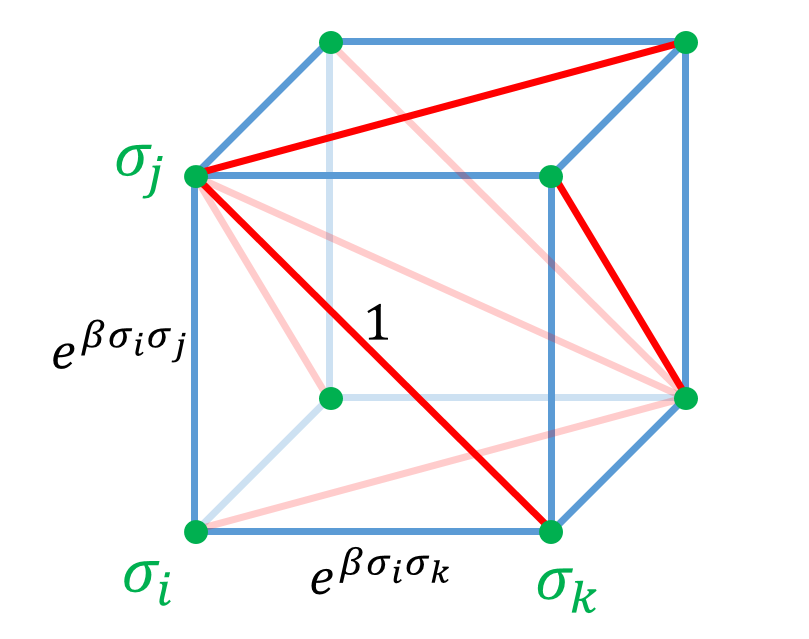
Figure 25: There are two types of boundary edges: the blue ones and the red ones. The boundary edges are determined by the bulk configuration $\{\sigma_{i}\}$, and we can read off their contribution to $\bigotimes_{e}\langle w_{e}|\{a\}_{\{x\}}\rangle$.

V.3 Boundary state under RG

The 3D boundary is divided into similar tetrahedra. Focusing on one tetrahedron, each face of it is shared by another tetrahedron. This inspires us to introduce face labels which will be contracted. And then we can construct a tensor network type wave function. Its building blocks are these tetrahedra. Given a tetrahedron labeled as shown in figure 26, it will contribute a tensor $u^{ijkl}(a,b,c)$, where $i,j,k,l$ are labels with dimension $N$ on the faces and $a,b,c$ are the objects (1 or -1) on the edges. One tetrahedron has 6 edges, but the objects on them are related by fusion rules, and where the bulk is a Dijkgraaf-Witten type lattice gauge theory, there are only 3 independent labels. So the tensor $u$ only has 3 arguments $a,b,c$.

In $u^{ijkl}(a,b,c)$, the order of indexes and the order of arguments are important. Now we introduce rules for reading off the tensor from the tetrahedron. The first step is to introduce arrows on the edges of the tetrahedra as shown in figure 27. Let us focus on one tetrahedron as shown in figure 28. We label its vertices by $0,1,2,3$ such that the arrows point from the small numbers to the large numbers. This label is unique. The red dot is always 0, and the purple dot is always 3. Then we label the $01,12,23$ edges by $a,b,c$ respectively. They are chosen as the 3 independent labels of edges. And we label the $012,023,013,123$ faces by $i,j,k,l$ respectively. The tensor corresponding to this tetrahedron is written as $u^{ijkl}(a,b,c)$.

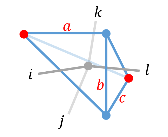
Figure 26: The labels on a tetrahedron. Here $a,b,c$ are the objects on the edges, and $i,j,k,l$ are labels on the faces. The grey lines here are for clear indication of the faces.

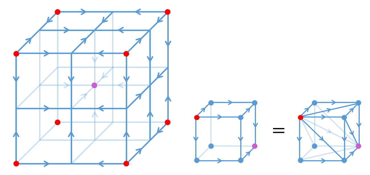
Figure 27: Introduce arrows to the edges of the tetrahedra. The center vertex of the $2\times 2\times 2$ cube is colored in purple now. Roughly speaking, the arrows point out from the red dots, and point to the purple dot. To avoid clutter, we don’t show all the arrows on the edges.

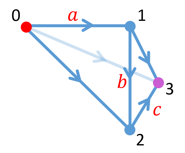
Figure 28: One tetrahedron with arrows introduced.

Each cube is divided into 6 tetrahedra. They are related with each other by 3D rotations and 3D reflections. So we assume that the tensors corresponding to them are the same $u$. And the tensor network type wave function is given by

$$\langle\Omega(u)|=\sum_{\{a\}}\sum_{i,j,k,l\dots}\dots u^{ijkl}(a_{1},a_{2},a_{3})\dots\langle\{a\}|,$$ (22)

where $\sum_{\{a\}}$ means the summation over all allowed boundary configurations, and $\sum_{i,j,k,l,\dots}$ is the summation over the labels of faces. Each tetrahedron on the boundary will contribute a $u$ tensor, and $\dots u^{ijkl}(a_{1},a_{2},a_{3})\dots$ is the product of these $u$ tensors. Now it becomes obvious that face labels $i,j,k,l,\dots$ are the indexes to be contracted.

We can recover the previous $\langle\Omega|$ in equation (18, 19) by choosing the $u^{ijkl}(a,b,c)$ to be

$$u^{ijkl}(a,b,c)=\left\{\begin{aligned} e^{\frac{\beta(a+2b+c)}{8}}&,&i=j=k=l=1,\\ 0&,&\textrm{Otherwise},\end{aligned}\right.$$ (23)

where $a,b,c$ take values $\{1,-1\}$ corresponding to objects $\{1,-1\}$. Let’s briefly explain how to obtain the above $u$. In (20), blue edges in figure 25 labeled by $a$ will contribute a factor $e^{\beta a}$ to $\langle\Omega|\Psi\rangle$. Note that $a,b,c$ in figure 29 correspond to the blue edges in figure 25. The edge labeled by $a$ is shared by 8 tetrahedra, and our choice of orientation is such that $a$ is the first argument (according to the rule in figure 28) in all of them. Similarly, the edge labeled by $b$ is shared by 4 tetrahedra, and $b$ is the second argument in all of them. Finally, the edge labeled by $c$ is shared by 8 tetrahedra, and $c$ is the third argument in all of them.

For simple illustration how to follow the flow of the boundary state (22) under repeated use of the above RG map, in the following we consider the case that the dimension of face labels is 1 i.e. $N=1$. And $u^{ijkl}(a,b,c)$ reduces to $u(a,b,c)$.

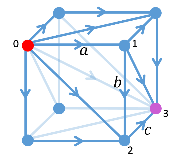
Figure 29: The 0123 tetrahedron in the cube. The labels $a,b,c$ lie on the previous blue edges of the cube.

As said before, one RG step consists of 3 steps. Let us recall the first step, now as shown in figure 30 with arrows introduced. The left hand side of figure 30 depicts the lattice before the RG step, and the right hand side the result of the RG step. The left and the right of figure 30 are respectively on the two boundaries of a 4D body which consists of eight 4-simplices. Now the 4D body becomes an operator $\mathcal{R}_{1}$ which consists of eight 4-cocycles $\alpha$ corresponding to these 4-simplices. And it maps the state defined on the left hand side to the state defined on the right hand side. The operator $\mathcal{R}_{1}$ imposes that edges forming a triangle have to product to the identity. For example, in the 4-simplex $09m21$ there is a face $09m$, and we should have $a_{0m}a_{9m}=a_{09}$ where $a_{0m}$ is the object on the edge $0m$.

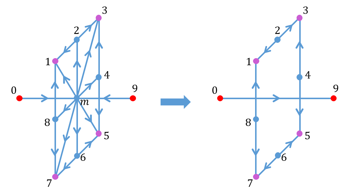
Figure 30: The first step, first illustrated in figure 19, now with arrows introduced. Here we relabel the vertices for convenience. These labels are just for indicating edges and faces. The purple dots are centers of $2\times 2\times 2$ cubes.

To satisfy the fusion rules, on the right hand side of figure 30 there are 9 independent labels which are chosen as $a_{01},a_{02},a_{03},a_{04},a_{05},a_{06},a_{07},a_{08},a_{09}$. Then the labels on other edges are fixed by them according to the fusion rules. For example $a_{21}=a_{02}a_{01}$. And the state defined on the right hand side takes the form

$$\sum_{a_{01},a_{02},\dots,a_{09}}\mathcal{M}^{R}_{1}(a_{01},a_{02},\dots,a_{09})\langle a_{01},a_{02},\dots,a_{09}|.$$ (24)

On the left of figure 30, there is one extra vertex $m$. Compared to the right, there is an extra independent edge degree of freedom $a_{0m}$. Given $a_{0m},a_{01},a_{02},a_{03},a_{04},a_{05},a_{06},a_{07},a_{08},a_{09}$, all the labels on the left hand side can be fixed. For example, $a_{9m}=a_{09}a_{0m}$ when we consider the face $09m$. The state defined on the left hand side takes the form

$$\sum_{a_{0m},a_{01},\dots,a_{09}}\mathcal{M}^{L}_{1}(a_{0m},a_{01},\dots,a_{09})\langle a_{0m},a_{01},\dots,a_{09}|.$$ (25)

Each tetrahedron will contribute a $u$ tensor. And we can read off $\mathcal{M}^{L}_{1}$ as

$$\mathcal{M}^{L}_{1} = u(a_{0m},a_{m2},a_{21})u(a_{0m},a_{m2},a_{23})u(a_{0m},a_{m4},a_{43})$$ (26)

$$\times u(a_{0m},a_{m4},a_{45})u(a_{0m},a_{m6},a_{65})u(a_{0m},a_{m6},a_{67})$$

$$\times u(a_{0m},a_{m8},a_{87})u(a_{0m},a_{m8},a_{81})u(a_{9m},a_{m2},a_{21})$$

$$\times u(a_{9m},a_{m2},a_{23})u(a_{9m},a_{m4},a_{43})u(a_{9m},a_{m4},a_{45})$$

$$\times u(a_{9m},a_{m6},a_{65})u(a_{9m},a_{m6},a_{67})u(a_{9m},a_{m8},a_{87})$$

$$\times u(a_{9m},a_{m8},a_{81}).$$

Here all the $a$’s can be expressed by $a_{0m}$, $a_{01}$,$a_{02}$,$\dots$,$a_{09}$. So the arguments of $\mathcal{M}^{L}_{1}$ are exactly $a_{0m}$,$a_{01}$,$a_{02}$,$\dots$,$a_{09}$. $\mathcal{M}^{R}_{1}$ and $\mathcal{M}^{L}_{1}$ are related under RG by

$$\mathcal{M}^{R}_{1}(a_{01},a_{02},\dots,a_{09})=\sum_{a_{0m}}\mathcal{M}^{L}_{1}(a_{0m},a_{01},a_{02},\dots,a_{09}).$$ (27)

When the labels $a_{01}$,$a_{02}$,$\dots$,$a_{09}$ of $\mathcal{M}^{R}_{1}$ are given, the labels $a_{01}$,$a_{02}$,$\dots$,$a_{09}$ in $\mathcal{M}^{L}_{1}$ are fixed. The edge $a_{0m}$ is an interior edge now buried between the left boundary condition and the RG operator $\mathcal{R}_{1}$, which should thus be summed over. In the 3+1 D toric code model, the RG operator is unity where fusion constraints on each face are satisfied.

In the 3D case, we follow the RG flow by performing an SVD to convert the boundary condition into a local form after every RG step as depicted in figure 11. We pursue a similar procedure here. But instead of breaking the blocked wavefunction (24) into two pieces, we need to break it into 8 pieces, one attached to each remaining tetrahedron on the right hand side of figure 30. Assume that after the break-up, each tetrahedron on the right hand side of figure 30 is attached to a tensor $v(a,b,c)$ . We denote the state constructed from $v(a,b,c)$ as

$$\sum_{a_{01},a_{02},\dots,a_{09}}\widetilde{\mathcal{M}}^{R}_{1}(a_{01},a_{02},\dots,a_{09})\langle a_{01},a_{02},\dots,a_{09}|,$$ (28)

where $\widetilde{\mathcal{M}}^{R}_{1}$ is given by

$$\widetilde{\mathcal{M}}^{R}_{1} = v(a_{09},a_{92},a_{21})v(a_{09},a_{92},a_{23})v(a_{09},a_{94},a_{43})$$ (29)

$$\times v(a_{09},a_{94},a_{45})v(a_{09},a_{96},a_{65})v(a_{09},a_{96},a_{67})$$

$$\times v(a_{09},a_{98},a_{87})v(a_{09},a_{98},a_{81}).$$

Here all the $a$’s can be expressed by $a_{01},a_{02},\dots,a_{09}$. So the arguments of $\widetilde{\mathcal{M}}^{R}_{1}$ are exactly $a_{01},a_{02},\dots,a_{09}$. Insisting that the face-degrees of freedom remain cut-downed to 1-dimensional (which is imposed by hand when we pick the tensor $v(a,b,c)$ to carry no extra indices attached to the faces), it is generically not possible to reproduce $\mathcal{M}^{R}_{1}$ precisely. We will try to optimise $v(a,b,c)$ such that

$$\epsilon_{1}\equiv\sum_{a_{01},\dots,a_{09}}|\mathcal{M}^{R}_{1}(a_{01},\dots,a_{09})-\widetilde{\mathcal{M}}^{R}_{1}(a_{01},\dots,a_{09})|^{2}$$ (30)

is minimal. The optimisation is done numerically here. Once $v(a,b,c)$ is found, we normalize it to

$$v(a,b,c)\rightarrow\frac{v(a,b,c)}{\sqrt{\frac{1}{8}\sum_{a,b,c}|v(a,b,c)|^{2}}}.$$ (31)

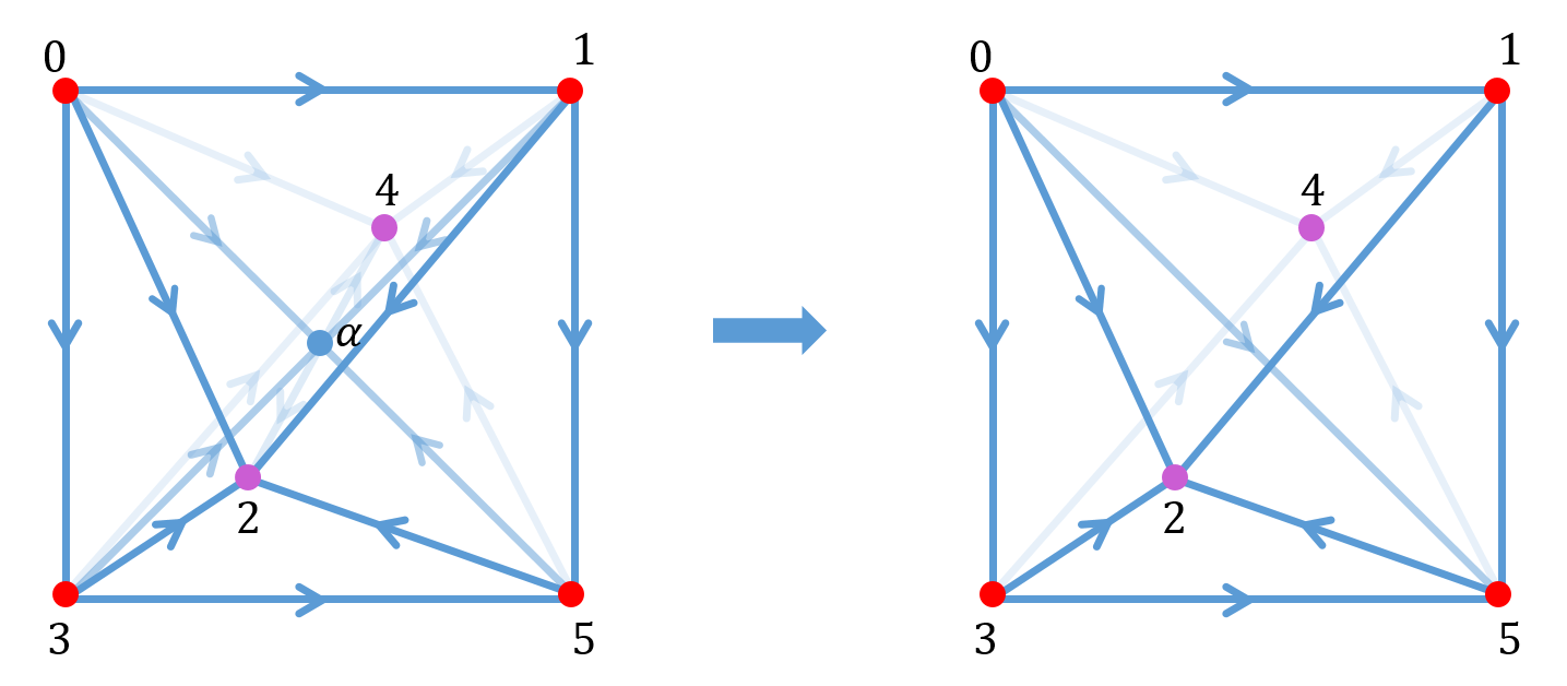
Figure 31: The second step with arrows introduced. Here we relabel the vertices for convenience. The purple dots are centers of $2\times 2\times 2$ cubes.

Now let us consider the second step. The procedure is similar. With arrows introduced the second step is shown in figure 31. On the right hand side there are 5 independent labels which are chosen as $a_{01},a_{02},a_{03},a_{04},a_{05}$. And the state defined on the right hand side takes the form

$$\sum_{a_{01},a_{02},\dots,a_{05}}\mathcal{M}^{R}_{2}(a_{01},a_{02},\dots,a_{05})\langle a_{01},a_{02},\dots,a_{05}|.$$ (32)

On the left hand side there are 6 independent labels which are chosen as $a_{0\alpha},a_{01},a_{02},a_{03},a_{04},a_{05}$. And the state defined on the left hand side takes the form

$$\sum_{a_{0\alpha},a_{01},\dots,a_{05}}\mathcal{M}^{L}_{2}(a_{0\alpha},a_{01},\dots,a_{05})\langle a_{0\alpha},a_{01},\dots,a_{05}|.$$ (33)

Previously we introduce $v(a,b,c)$ and approximate $\mathcal{M}^{R}_{1}$ by $\widetilde{\mathcal{M}}^{R}_{1}$. Now each tetrahedron on the left hand side will contribute $v(a,b,c)$. And we can read off $\mathcal{M}^{L}_{2}$ as

$$\mathcal{M}^{L}_{2} = v(a_{01},a_{1\alpha},a_{\alpha 2})v(a_{03},a_{3\alpha},a_{\alpha 2})v(a_{15},a_{5\alpha},a_{\alpha 2})$$ (34)

$$\times v(a_{35},a_{5\alpha},a_{\alpha 2})v(a_{01},a_{1\alpha},a_{\alpha 4})v(a_{03},a_{3\alpha},a_{\alpha 4})$$

$$\times v(a_{15},a_{5\alpha},a_{\alpha 4})v(a_{35},a_{5\alpha},a_{\alpha 4}).$$

Here all the $a$’s can be expressed by $a_{0\alpha}$,$a_{01}$,$a_{02}$,$\dots$,$a_{05}$. So the arguments of $\mathcal{M}^{L}_{2}$ are exactly $a_{0\alpha}$,$a_{01}$,$a_{02}$,$\dots$,$a_{05}$. And we can obtain $\mathcal{M}^{R}_{2}$ from $\mathcal{M}^{L}_{2}$ by the formula

$$\mathcal{M}^{R}_{2}(a_{01},a_{02},\dots,a_{05})=\sum_{a_{0\alpha}}\mathcal{M}^{L}_{2}(a_{0\alpha},a_{01},a_{02},\dots,a_{05}).$$ (35)

Now we have to repeat the procedure above to break up $\mathcal{M}^{R}_{2}$. We introduce another new function $t(a,b,c)$ to the tetrahedra on the right hand side of figure 31 from which we define the state

$$\sum_{a_{01},a_{02},\dots,\alpha_{05}}\widetilde{\mathcal{M}}^{R}_{2}(a_{01},a_{02},\dots,a_{05})\langle a_{01},a_{02},\dots,a_{05}|,$$ (36)

where $\widetilde{\mathcal{M}}^{R}_{2}$ is given by

$$\widetilde{\mathcal{M}}^{R}_{2} = t(a_{01},a_{15},a_{52})t(a_{03},a_{35},a_{52})t(a_{01},a_{15},a_{54})$$ (37)

$$\times t(a_{03},a_{35},a_{54}).$$

Here all the $a$’s can be expressed by $a_{01},a_{02},\dots,a_{05}$. So the arguments of $\widetilde{\mathcal{M}}^{R}_{2}$ are exactly $a_{01},a_{02},\dots,a_{05}$. Now we would like to find the best $t(a,b,c)$ to approximate $\mathcal{M}^{R}_{2}$ by $\widetilde{\mathcal{M}}^{R}_{2}$ such that

$$\epsilon_{2}\equiv\sum_{a_{01},\dots,a_{05}}|\mathcal{M}^{R}_{2}(a_{01},\dots,a_{05})-\widetilde{\mathcal{M}}^{R}_{2}(a_{01},\dots,a_{05})|^{2}$$ (38)

is minimal. This is again achieved by numerical method. Once $t(a,b,c)$ is found, we normalize it to

$$t(a,b,c)\rightarrow\frac{t(a,b,c)}{\sqrt{\frac{1}{8}\sum_{a,b,c}|t(a,b,c)|^{2}}}.$$ (39)

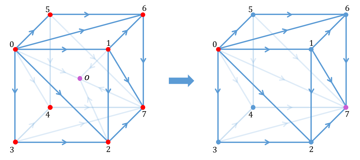
Figure 32: The third step with arrows introduced. Here we relabel the vertices for convenience. Vertex $o$ is the center of the original $2\times 2\times 2$ cube, and vertex $7$ becomes the center of the coarse grained $2\times 2\times 2$ cube.

We would then proceed to the third step. With arrows introduced the third step is shown in figure 32. On the right hand side there are 7 independent labels which are chosen as $a_{01}$,$a_{02}$,$a_{03}$,$a_{04}$,$a_{05}$,$a_{06}$,$a_{07}$. And the state defined on the right hand side takes the form

$$\sum_{a_{01},a_{02},\dots,a_{07}}\mathcal{M}^{R}_{3}(a_{01},a_{02},\dots,a_{07})\langle a_{01},a_{02},\dots,a_{07}|.$$ (40)

On the left hand side there are 8 independent labels which are chosen as $a_{0o},a_{01},a_{02},\dots,a_{07}$. And the state defined on the left hand side takes the form

$$\sum_{a_{0o},a_{01},\dots,a_{07}}\mathcal{M}^{L}_{3}(a_{0o},a_{01},\dots,a_{07})\langle a_{0o},a_{01},\dots,a_{07}|.$$ (41)

Previously we introduce $t(a,b,c)$ and approximate $\mathcal{M}^{R}_{2}$ by $\widetilde{\mathcal{M}}^{R}_{2}$. Now each tetrahedron on the left hand side of figure 32 will contribute $t(a,b,c)$. And we can read off $\mathcal{M}^{L}_{3}$ as

$$\mathcal{M}^{L}_{3} = t(a_{01},a_{12},a_{2o})t(a_{03},a_{32},a_{2o})t(a_{01},a_{16},a_{6o})\times$$ (42)

$$t(a_{05},a_{56},a_{6o})t(a_{05},a_{54},a_{4o})t(a_{03},a_{34},a_{4o})\times$$

$$t(a_{12},a_{27},a_{7o})t(a_{16},a_{67},a_{7o})t(a_{56},a_{67},a_{7o})\times$$

$$t(a_{54},a_{47},a_{7o})t(a_{32},a_{27},a_{7o})t(a_{34},a_{47},a_{7o})$$

Here all the $a$’s can be expressed by $a_{0o},a_{01},a_{02},\dots,a_{07}$. So the arguments of $\mathcal{M}^{L}_{3}$ are exactly $a_{0o},a_{01},a_{02},\dots,a_{07}$. And we can obtain $\mathcal{M}^{R}_{3}$ from $\mathcal{M}^{L}_{3}$ by the formula

$$\mathcal{M}^{R}_{3}(a_{01},a_{02},\dots,a_{07})=\sum_{a_{0o}}\mathcal{M}^{L}_{3}(a_{0o},a_{01},a_{02},\dots,a_{07}).$$ (43)

Now we introduce a new function $u^{(1)}(a,b,c)$ to the tetrahedra on the right hand side of figure 32. And we can obtain the state

$$\sum_{a_{01},a_{02},\dots,\alpha_{07}}\widetilde{\mathcal{M}}^{R}_{3}(a_{01},a_{02},\dots,a_{07})\langle a_{01},a_{02},\dots,a_{07}|,$$ (44)

where $\widetilde{\mathcal{M}}^{R}_{3}$ is given by

$$\widetilde{\mathcal{M}}^{R}_{3} = u^{(1)}(a_{01},a_{12},a_{27})u^{(1)}(a_{01},a_{16},a_{67})$$ (45)

$$\times u^{(1)}(a_{05},a_{56},a_{67})u^{(1)}(a_{05},a_{54},a_{47})$$

$$\times u^{(1)}(a_{03},a_{34},a_{47})u^{(1)}(a_{03},a_{32},a_{27}).$$

Here all the $a$’s can be expressed by $a_{01},a_{02},\dots,a_{07}$. So the arguments of $\widetilde{\mathcal{M}}^{R}_{3}$ are exactly $a_{01},a_{02},\dots,a_{07}$. Now we would like to find the best $u^{(1)}(a,b,c)$ to approximate $\mathcal{M}^{R}_{3}$ by $\widetilde{\mathcal{M}}^{R}_{3}$ such that

$$\epsilon_{3}\equiv\sum_{a_{01},\dots,a_{07}}|\mathcal{M}^{R}_{3}(a_{01},\dots,a_{07})-\widetilde{\mathcal{M}}^{R}_{3}(a_{01},\dots,a_{07})|^{2}$$ (46)

is minimal. This is achieved by numerical method. Once $u^{(1)}(a,b,c)$ is found, we normalize it to

$$u^{(1)}(a,b,c)\rightarrow\frac{u^{(1)}(a,b,c)}{\sqrt{\frac{1}{8}\sum_{a,b,c}|u^{(1)}(a,b,c)|^{2}}}.$$ (47)

We can note that after one RG step, the wave function becomes

$$\langle\Omega(u^{(1)})|=\sum_{\{a\}}\dots u^{(1)}(a_{1},a_{2},a_{3})\dots\langle\{a\}|,$$ (48)

which takes the same form as the origin wave function in (22). The only difference is replacing $u(a,b,c)$ by $u^{(1)}(a,b,c)$. And we can iterate this RG step. After $n$ RG steps, we would get $u^{(n)}(a,b,c)$, and the wave function is

$$\langle\Omega(u^{(n)})|=\sum_{\{a\}}\dots u^{(n)}(a_{1},a_{2},a_{3})\dots\langle\{a\}|.$$ (49)

We expect that when $n$ is large enough, $u^{(n)}(a,b,c)$ will arrive at some fixed point and $\langle\Omega(u^{(n)})|$ becomes one of the fixed point wave functions.

Recall that when we choose $u(a,b,c)$ as

$$u_{\beta}(a,b,c)\equiv e^{\frac{\beta(a+2b+c)}{8}},$$ (50)

the overlap $\langle\Omega|\Psi\rangle_{\mathcal{M}}$ is the partition function of 3D Ising model. And it is interesting to investigate where $u_{\beta}(a,b,c)$ will flow to. There is a parameter $\beta$ in $u_{\beta}(a,b,c)$. We find that when changing $\beta$, the $u_{\beta}(a,b,c)$ will flow to different fixed points. And it is easy to check that $u_{0}(a,b,c)$ and $u_{\infty}(a,b,c)$ are two fixed points. Our numerical result shows that when $0\leq\beta\leq 0.27$, $u_{\beta}(a,b,c)$ will flow to the fixed point $u_{0}(a,b,c)$. However when $\beta=0.28$, our numerical method breaks down since the errors $\epsilon_{1},\epsilon_{2},\epsilon_{3}$ wouldn’t converge to 0 when $n$ becomes larger. And this suggests that something special happens in the range $\beta\in(0.27,0.28)$ – which is a signature of getting close to the critical point of the 3D Ising model. In literature (See for example for a collection of numerical results in Hasenbusch (2010)), the critical point of the 3D Ising model is $\beta_{c}=0.22165463(8)$. Our result is surprisingly good with a choice of face bond dimension truncated down to $N=1$. Increasing the face dimension $N$ should improve our accuracy. This will be demonstrated in a forth-coming paperJi et al. .

VI Tensor Network reconstruction of AdS/CFT? – Some Numerics

We have proposed construction of RG operators analytically from topological data of $D+1$ dimensional topological lattice model, and demonstrated explicitly in $D+1=2,3,4$ dimensions in a family of models. Since these are operators responsible for blocking, repeated concatenation of them $\lim_{N\to\infty}U(\mathcal{C})^{N}$ produces a MERA like network, which is thus an analytic holographic network, which, with the right boundary condition that is itself the fixed point or one that could flow to the fixed point, describes exact CFT’s. We have given examples which map to well known 2D integrable models, or the 3D Ising model.

These strange correlators bear a close resemblance to the p-adic tensor network that reproduces many aspects of the p-adic AdS/CFT dictionary Hung et al. (2019); Chen et al. (2021b, a).The resemblance lies in the fact that the bulk of the tensor network is characterized by an associative algebra (the fusion algebra of the CFT operators) and this is generalized to (higher) fusion categories in the general construction in this paper. The p-adic tensor network that reproduces the p-adic CFT partition function also comes in the form of a strange correlator, such that at the fixed point, the boundary state is an eigenstate of the bulk holographic network. It is thus tempting that the current holographic network may bear resemblance to the AdS/CFT correspondence.

VI.1 Bulk-Boundary Correlators

For simplicity, we work with the 2D Ising CFT that can be obtained from the $SU(2)_{3}$. The CFT has a small central charge and is not expected to have a semi-classical gravitational dual. However we would like to see how such a broad-brush would work. We computed numerically two point functions where one operator is inserted at the UV layer given by figure 12, and the other at the $n$-th layer of the holographic network. i.e.

$$\langle\mathcal{O}(n=0,x=y=0)\mathcal{O}(n,x,y)\rangle$$

$$=\langle\Omega(T_{\Lambda_{0}})|\sigma^{z}(x=y=0)U^{n}(\mathcal{C})\sigma^{z}(x,y)U^{n+1}(\mathcal{C})\cdots|\Psi\rangle$$

$$=\langle\Omega(T_{\Lambda_{0}})|\sigma^{z}(x=y=0)U^{n}(\mathcal{C})\sigma^{z}(x,y)|\Psi_{\Lambda_{n}}\rangle.$$ (51)

The result is illustrated in figure 33. In the bottom plot, the plots at different $n$ collapse to the same plot in a more convincing way than the top plot, promisingly, suggesting that the “bulk-boundary propagator” in this holographic network is indeed given by $[z/(z^{2}+x^{2})]^{\Delta}$. This is, admittedly, not yet conclusive before we can explore more models and more propagators of different conformal dimensions.

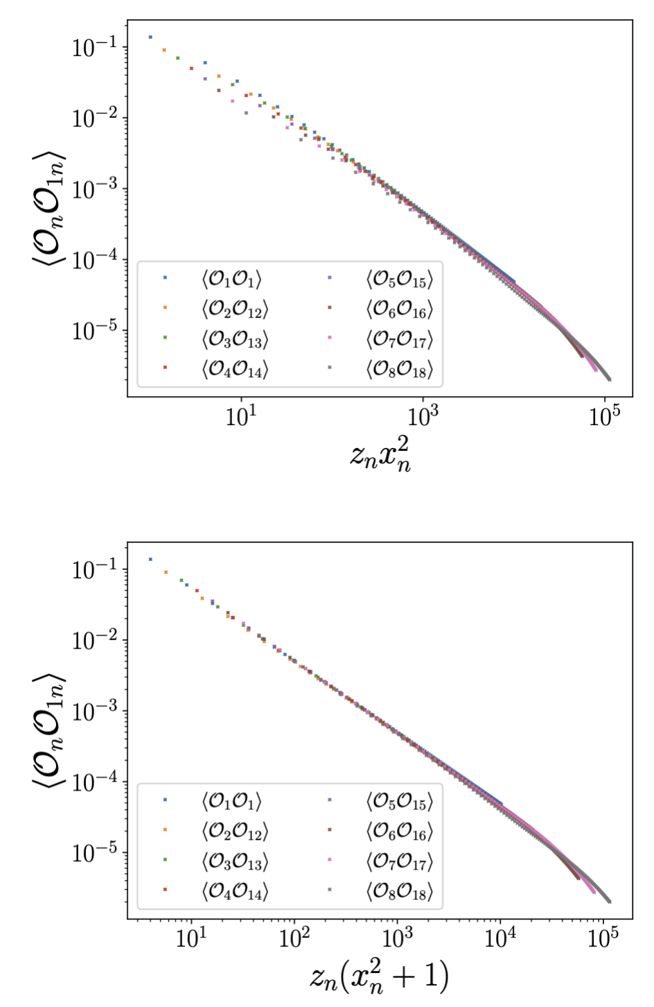
Figure 33: $\mathcal{O}_{n}$ denotes operator insertion at the $n$-th layer. $\mathcal{O}_{1n}$ corresponds to operation insertion at layer 1 (which is subsequently blocked with nearby tensors to the $n$-th layer – for computational convenience). $\langle\mathcal{O}_{n}\mathcal{O}_{1n}\rangle$ is thus $\langle\mathcal{O}_{n}\mathcal{O}_{1}\rangle$. We make a log-log plot against $z_{n}x_{n}^{2}$ at the top, and $z_{n}(1+x_{n}^{2})$ in the bottom. Here, $z_{n}=(\sqrt{2})^{n-1}$ and $x_{1}=z_{n}x_{n}$. The AdS/CFT dictionary would suggest that $\langle\mathcal{O}_{n}\mathcal{O}_{1}\rangle=(z_{n}(x_{n}^{2}+1))^{-\Delta}$, where $\Delta$ is the conformal dimension of the CFT primary operator $\mathcal{O}_{1}$. All the plots of different $n$ collapse very nicely to the same line in the bottom plot.

VI.2 Reconstruction Wedge

It is not hard to obtain the entanglement wedge, or reconstruction wedge of any edge in the interior. In the tree RG network in 2D depicted in figure 3, the entanglement wedge at the UV boundary is self-explanatory. In the case of a 3D bulk, the holographic network is depicted in figure 34. It is a projection of the 3D structure into two dimensions. To reconstruct action of edges in the interior layer from the UV layer, the UV degrees of freedom involved correspond to edges of triangles in the UV layer that appear to be contained inside the triangle in the interior layer concerned. The explicit transformation that converts an operator in the bulk into an operator from the UV boundary requires construction of the inverse of the holographic networks. This can be readily done using the orthogonality condition given by

$$\sum_{y}d_{y}\left[\begin{tabular}[]{ccc}$a$&$b$&$x$\\ $c$&$d$&$y$\end{tabular}\right]\left[\begin{tabular}[]{ccc}$a$&$b$&$x^{\prime}$\\ $c$&$d$&$y$\end{tabular}\right]=\frac{\delta_{xx^{\prime}}N^{x}_{ab}N^{x}_{cd}}{d_{x}}$$ (52)

.

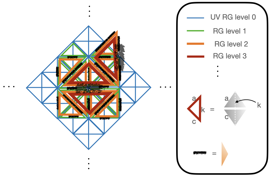
Figure 34: The picture depicts layers of tetrahedra on top of each other, implementing the RG process discussed in figure 6, where two triangles are merged into one recursively. These layers of triangles are projections of the tetrahedron that is color - coded depending on the layer. The larger triangles contain smaller triangles from UV layers that eventually blocked into them. The entanglement wedge of any edge belonging to any triangle at a given layer is given by all the smaller triangles contained inside this triangle.

VII Conclusions and Outlook

In this paper, we constructed an exact holographic network that descends from coarse graining a topological wave-function. These holographic networks correspond to RG operators that preserve a given set of “categorical symmetries” associated to the TQFT in $D+1$ dimensions. Each fixed point of the RG operator determines either a TQFT or a CFT in $D$ dimensions that preserve the categorical symmetry concerned (or spontaneousely breakinng part of it). For bulk TQFTs in the family of Dijkgraaf-Witten models in arbitrary dimensions or Turaev type in 3 dimensions, fixed points describing TQFT’s are constructed using the (co-) product of (higher-) Frobenius algebra of the input fusion category $\mathcal{C}$. Fixed points corresponding to CFTs can be obtained by looking for phase transitions between topological fixed points. We illustrated these ideas in $1\leq D\leq 3$. At $D=2$, we find that critical couplings of $SU(2)_{k}$ models can be recovered to at least one significant figure with very small bond-dimension compared to known theoretical values. We note that our numerical procedure can in fact also efficiently generate the Frobenius algebra as topological fixed points, recovering known analytic results. We also show that the $3D$ Ising model can be taken as a strange correlator with the $4D$ toric code, and the critical temperature can be obtained by looking for phase transition points between two topological fixed points of the corresponding RG operator corresponding to the smooth and rough boundaries associated to two higher Frobenius algebra. We note that in the literature, it is known that different Frobenius algebras in the input category produce isomorphic/equivalent condensation Hu et al. (2017), which is often taken to be the same spatial boundary condition. In our construction, it should be evident that there are phase transitions (such as the 2D Ising model) between algebras considered to be physically the same in Hu et al. (2017). It suggests that isomorphic/equivalent condensation algebras should be considered as physically distinct in one lower dimension.

We briefly look into the possibility of recovering some features of the AdS/CFT dictionary, such as the bulk-boundary propagator. The numerical result is, encouragingly, compatible with the AdS/CFT dictionary but not yet conclusive.

The approach we adopted and developed to construct CFT partition functions via RG operators following from TQFT in one higher dimensions can be considered as an explicit realization of the Wick-rotation and holographic dualities discussed in Freed and Teleman (2018); Lootens et al. (2021); Ji and Wen (2020); Kong et al. (2020a); Albert et al. (2021); Chatterjee and Wen (2022a, b); Liu and Ji (2022); Kong and Zheng (2018, 2020, 2021, 2022); Kong et al. (2020b, 2022); Xu and Zhang (2022); Aasen et al. (2016); Vanhove et al. (2018); Lootens et al. (2019); Gaiotto and Kulp (2021); Bhardwaj et al. (2020); Apruzzi et al. (2021); Moradi et al. (2022). In the examples at hand, it is possible to extract systematically from the topological skeleton also the “meat” of the critical point – allowing one to identify the critical coupling and recovering the actual CFT partition function even beyond 1+1 D CFTs. The philosophy is closely related to the approach taken in Chatterjee and Wen (2022b, a) to classify critical points through phase transitions between topological fixed points, the latter of which described by condensation algebra in the topological order (or the output category) – although the current construction is based on Frobenius algebra of the input category.

Our explicit realization should open the door to constructing more novel CFTs in general dimensions. At present, we are trying to identify the nature of the tricritical point that should be a 2D CFT, and we would like to construct more examples, both 2D and 3D. To our knowledge, our algorithm for searching for 2+1D topological fixed points of the 4D RG operator is essentially a first tensor network renormalization method applied to a 3D tensor network. We have since improved the algorithm to allow for larger bond dimensions. And these results would appear in a forth-coming paper Ji et al. . We should also be able to construct partition functions of (1+1 D) spin CFT by considering phase transitions between super Frobenius algebra previousely used to characterize fermionic spatial boundary conditions following from fermionic anyon condensations Aasen et al. (2019); Gaiotto and Kapustin (2016); Wan and Wang (2017); Lou et al. (2021). This will be left for future work.

We explored whether the holographic duality exhibited in the current context is related to the AdS/CFT correspondence in its usual sense. The result is not incompatible, but certainly requires further scrutiny, which is currently underway.

Acknowledgements.— LYH acknowledges the support of NSFC (Grant No. 11922502, 11875111) and the Shanghai Municipal Science and Technology Major Project (Shanghai Grant No.2019SHZDZX01), and Perimeter Institute for hospitality as a part of the Emmy Noether Fellowship programme. Part of this work was instigated in KITP during the program qgravity20. LC acknowledges support of NSFC (Grant No. 12047515). We thank Bartek Czech, Babak Haghighat, Binxin Lao, Jiaqi Lou, Han Ma, Xiao-Liang Qi, Frank Verstraete, Gabriel Wong and Qifeng Wu for useful discussions. We thank Liang Kong in particular for discussions and detailed comments to our draft.

Appendix A Fixed point wavefunctions of 2D Dijkgraaf-Witten RG operator

In DW theory of group $G$, the basis of state at each site is given by $|g\rangle$, $g\in G$. We can alternatively use irreducible representations of the group to construct a basis. They are related by

$$|\mu,a,b\rangle=\sqrt{\frac{|\mu|}{|G|}}\mathcal{N}_{\mu}\sum_{g}\rho^{\mu}_{ab}(g)|g\rangle,$$ (53)

where $\mu$ labels an irreducible representation, and $|\mu|$ is the dimension of the representation. Therefore we can take $\otimes_{i}^{N}\rho^{\mu}(g)_{ab}$ as a complete basis for wavefunctions of $N$ sites. Consider the action of the RG operator described in figure 3 and that the group cohomology is trivial. A triangle is thus equal to $\delta_{g_{1}g_{2},h}$. We can thus consider pairs of sites. Summation of a basis wave-function with the triangle with given output $h=g_{1}g_{2}$ gives

$$\sum_{g_{1}\in G}\rho^{\mu}_{a_{1}b_{1}}(g_{1})\rho^{\nu}_{a_{2}b_{2}}(g_{1}^{-1}h)=\frac{|G|}{|\mu|}\delta_{\mu\nu}\delta_{a_{1}c}\delta_{b_{1}a_{2}}\rho^{\mu}_{cb_{2}}(h)$$

$$=\frac{1}{|\mu|}\delta_{\mu\nu}\delta_{b_{1}a_{2}}\sum_{g_{1}g_{2}=h}\sum_{m}\rho^{\mu}_{a_{1}m}(g_{1})\rho^{\mu}_{mb_{2}}(g_{2}).$$ (54)

This suggests that for whatever wave-function we started with, after the action of a triangle (a single 3-point vertex of the RG operator) on neighbouring sites, the wave-function would be projected into the direction corresponding to the same representation on neighbouring sites contracted with each other. Therefore upon multiple layers of the RG operator acting on any given boundary state, it would be projected into the form of (8) up to an overall normalization. The most general fixed point would be a direct sum of these fixed point solutions.

We note that the choice of RG operator is not unique. For example, one can construct an RG operator that would carry a form that is more closely resembling the MERA tensor network. It corresponds to a triangulation that is depicted in figure 35. The most general fixed point for arbitrary $G$ but trivial $\alpha$ however remains the same as in (8), following a consideration analogous to (54).

Figure 35: A different choice of the RG operator $\mathcal{R}$ compared to $U(G,\alpha)$ in figure 3. Here an extra pair of triangle playing the role of “disentangler” is inserted between triangles that are responsible for blocking.

Appendix B Frobenius algebra in $n$ D Dijkgraaf-Witten Models

Let’s consider n-dimension DW theories characterized by group G as an example. The n-dimension body is triangulated into n-simplexes, where each edge is labeled by a group element $g_{i}\in G,$ and the n-simplex is assigned a value $\alpha(g_{1},g_{2},\dots,g_{n})\in H^{n}(G,U(1))$, where $H^{n}(G,U(1))$ denotes the n-cohomology, and $g_{1},g_{2},\dots,g_{n}$ are the labels on the edges $i_{0}i_{1},i_{1}i_{2},\dots,i_{n-1}i_{n}$ if the vertices of the n-simplex are $i_{0},i_{1},i_{2},\dots,i_{n}$ with $i_{0}<i_{1}<i_{2}<\dots<i_{n}$. Since $\alpha(g_{1},g_{2},\dots,g_{n})\in H^{n}(G,U(1))$, it satisfies the cocycle condition $d\alpha=1$, where

$$d\alpha(g_{0},g_{1},\dots,g_{n})\equiv\prod_{i=0}^{n+1}\alpha(\dots,g_{i-2},g_{i-1}g_{i},g_{i+1},\dots)^{(-1)^{i}}.$$ (55)

This condition guarantees that the partition function of the closed n-dimension manifold is invariant under different triangulations.

When the n-dimension body has a boundary, to retain its topological nature, we should construct a partition function which is invariant under different triangulations of both the bulk and the boundary. The boundary is triangulated into (n-1)-simplexes, where each edge is labeled by a group element $h_{i}\in H\subseteq G,$ and the (n-1)-simplex is assigned a value $\beta(h_{1},h_{2},\dots,h_{n-1})$, where $h_{1},h_{2},\dots,h_{n-1}$ are the labels on the edges $i_{0}i_{1},i_{1}i_{2},\dots,i_{n-2}i_{n-1}$ if the vertices of the (n-1)-simplex are $i_{0},i_{1},i_{2},\dots,i_{n-1}$ with $i_{0}<i_{1}<i_{2}<\dots<i_{n-1}$. The partition function takes the form

$$Z=\sum_{\{g_{i}\}}\sum_{\{h_{i}\}}\prod_{\Delta_{n}}\alpha_{\Delta_{n}}\prod_{\Delta_{n-1}}\beta_{\Delta_{n-1}},$$ (56)

where the summations are over all allowed configurations, each n-simplex $\Delta_{n}$ in the bulk contributes $\alpha_{\Delta_{n}}$, and each (n-1)-simplex $\Delta_{n-1}$ on the boundary contributes $\beta_{\Delta_{n-1}}$. To make this partition function invariant under different triangulations of both the bulk and the boundary, we should have

$$\alpha d\beta\equiv$$

$$\alpha(h_{0},h_{1},\dots,h_{n-1})\prod_{i=0}^{n}\beta(\dots,h_{i-2},h_{i-1}h_{i},h_{i+1},\dots)^{(-1)^{i}}$$

$$=1.$$ (57)

We note that both the fixed point solutions for the 4D DW bulk belongs to this class, where $\beta$ is used to construct the boundary state $\langle\Omega|$. In the 2D case, the MPS representation of fixed point boundary states $\langle\Omega|$ we have obtained generally contain auxiliary indices – geometrically we are still attaching a generalized $\beta$ to each edge at the boundary with auxiliary indices attached to the vertices at the end of the edge such that two edges sharing the same vertex would have their shared auxiliary index contracted. We note however in this generalized sense they are still solution to equation B.

References

- Aasen et al. (2016) D. Aasen, R. S. K. Mong, and P. Fendley, J. Phys. A 49, 354001 (2016), arXiv:1601.07185 [cond-mat.stat-mech] .
- Aasen et al. (2020) D. Aasen, P. Fendley, and R. S. K. Mong, (2020), arXiv:2008.08598 [cond-mat.stat-mech] .
- Vanhove et al. (2018) R. Vanhove, M. Bal, D. J. Williamson, N. Bultinck, J. Haegeman, and F. Verstraete, Phys. Rev. Lett. 121, 177203 (2018).
- Bhardwaj and Tachikawa (2018) L. Bhardwaj and Y. Tachikawa, JHEP 03, 189 (2018), arXiv:1704.02330 [hep-th] .
- Chang et al. (2019) C.-M. Chang, Y.-H. Lin, S.-H. Shao, Y. Wang, and X. Yin, JHEP 01, 026 (2019), arXiv:1802.04445 [hep-th] .
- Thorngren and Wang (2019) R. Thorngren and Y. Wang, (2019), arXiv:1912.02817 [hep-th] .
- Thorngren and Wang (2021) R. Thorngren and Y. Wang, (2021), arXiv:2106.12577 [hep-th] .
- Ji and Wen (2020) W. Ji and X.-G. Wen, Phys. Rev. Res. 2, 033417 (2020), arXiv:1912.13492 [cond-mat.str-el] .
- Kong et al. (2020a) L. Kong, T. Lan, X.-G. Wen, Z.-H. Zhang, and H. Zheng, Phys. Rev. Res. 2, 043086 (2020a), arXiv:2005.14178 [cond-mat.str-el] .
- Albert et al. (2021) V. V. Albert, D. Aasen, W. Xu, W. Ji, J. Alicea, and J. Preskill, (2021), arXiv:2111.12096 [cond-mat.str-el] .
- Chatterjee and Wen (2022a) A. Chatterjee and X.-G. Wen, (2022a), arXiv:2203.03596 [cond-mat.str-el] .
- Liu and Ji (2022) S. Liu and W. Ji, (2022), arXiv:2208.09101 [cond-mat.str-el] .
- Lootens et al. (2021) L. Lootens, C. Delcamp, G. Ortiz, and F. Verstraete, (2021), arXiv:2112.09091 [quant-ph] .
- Freed and Teleman (2018) D. S. Freed and C. Teleman, (2018), arXiv:1806.00008 [math.AT] .
- Levin (2020) M. Levin, Commun. Math. Phys. 378, 1081 (2020), arXiv:1903.09028 [cond-mat.str-el] .
- Verlinde (1988) E. P. Verlinde, Nucl. Phys. B 300, 360 (1988).
- Petkova and Zuber (2001) V. B. Petkova and J. B. Zuber, Phys. Lett. B 504, 157 (2001), arXiv:hep-th/0011021 .
- Frohlich et al. (2007) J. Frohlich, J. Fuchs, I. Runkel, and C. Schweigert, Nucl. Phys. B 763, 354 (2007), arXiv:hep-th/0607247 .
- Frohlich et al. (2004) J. Frohlich, J. Fuchs, I. Runkel, and C. Schweigert, Phys. Rev. Lett. 93, 070601 (2004), arXiv:cond-mat/0404051 .
- Fuchs et al. (2002) J. Fuchs, I. Runkel, and C. Schweigert, Nucl. Phys. B 646, 353 (2002), arXiv:hep-th/0204148 .
- Fuchs et al. (2004a) J. Fuchs, I. Runkel, and C. Schweigert, Nucl. Phys. B 678, 511 (2004a), arXiv:hep-th/0306164 .
- Fuchs et al. (2004b) J. Fuchs, I. Runkel, and C. Schweigert, Nucl. Phys. B 694, 277 (2004b), arXiv:hep-th/0403157 .
- Fuchs et al. (2005) J. Fuchs, I. Runkel, and C. Schweigert, Nucl. Phys. B 715, 539 (2005), arXiv:hep-th/0412290 .
- Quella et al. (2007) T. Quella, I. Runkel, and G. M. T. Watts, JHEP 04, 095 (2007), arXiv:hep-th/0611296 .
- Fuchs et al. (2008) J. Fuchs, I. Runkel, and C. Schweigert, Appl. Categ. Struct. 16, 123 (2008), arXiv:math/0701223 .
- Fuchs et al. (2007) J. Fuchs, M. R. Gaberdiel, I. Runkel, and C. Schweigert, J. Phys. A 40, 11403 (2007), arXiv:0705.3129 [hep-th] .
- Bachas and Brunner (2008) C. Bachas and I. Brunner, JHEP 02, 085 (2008), arXiv:0712.0076 [hep-th] .
- Davydov et al. (2011) A. Davydov, L. Kong, and I. Runkel, , 71 (2011), arXiv:1107.0495 [math.QA] .
- Davydov et al. (2015) A. Davydov, L. Kong, and I. Runkel, Adv. Math. 285, 811 (2015), arXiv:1307.5956 [math.QA] .
- Kong et al. (2021) L. Kong, W. Yuan, and H. Zheng, Commun. Math. Phys. 381, 1409 (2021), arXiv:1912.13168 [math.QA] .
- Petkova (2010) V. B. Petkova, JHEP 04, 061 (2010), arXiv:0912.5535 [hep-th] .
- Carqueville and Runkel (2016) N. Carqueville and I. Runkel, Quantum Topol. 7, 203 (2016), arXiv:1210.6363 [math.QA] .
- Kitaev and Kong (2012) A. Kitaev and L. Kong, Commun. Math. Phys. 313, 351 (2012), arXiv:1104.5047 [cond-mat.str-el] .
- Brunner et al. (2014) I. Brunner, N. Carqueville, and D. Plencner, Proc. Symp. Pure Math. 88, 231 (2014), arXiv:1310.0062 [hep-th] .
- Petkova (2013) V. B. Petkova, Phys. Atom. Nucl. 76, 1268 (2013).
- Williamson et al. (2017) D. J. Williamson, N. Bultinck, and F. Verstraete, (2017), arXiv:1711.07982 [quant-ph] .
- Makabe and Watts (2017) I. Makabe and G. M. T. Watts, JHEP 09, 013 (2017), arXiv:1703.09148 [hep-th] .
- Thorngren (2020) R. Thorngren, Commun. Math. Phys. 378, 1775 (2020), arXiv:1810.04414 [cond-mat.str-el] .
- Ji et al. (2020) W. Ji, S.-H. Shao, and X.-G. Wen, Phys. Rev. Res. 2, 033317 (2020), arXiv:1909.01425 [cond-mat.str-el] .
- Lin and Shao (2021) Y.-H. Lin and S.-H. Shao, J. Phys. A 54, 065201 (2021), arXiv:1911.00042 [hep-th] .
- Chang and Lin (2021) C.-M. Chang and Y.-H. Lin, JHEP 10, 125 (2021), arXiv:2012.01429 [hep-th] .
- Huang et al. (2021a) T.-C. Huang, Y.-H. Lin, and S. Seifnashri, JHEP 12, 028 (2021a), arXiv:2110.02958 [hep-th] .
- Burbano et al. (2021) I. M. Burbano, J. Kulp, and J. Neuser, (2021), arXiv:2112.14323 [hep-th] .
- Brunner et al. (2015) I. Brunner, N. Carqueville, and D. Plencner, Commun. Math. Phys. 337, 429 (2015), arXiv:1404.7497 [hep-th] .
- Carqueville et al. (2020) N. Carqueville, C. Meusburger, and G. Schaumann, Adv. Math. 364, 107024 (2020), arXiv:1603.01171 [math.QA] .
- Carqueville et al. (2019) N. Carqueville, I. Runkel, and G. Schaumann, Geom. Topol. 23, 781 (2019), arXiv:1705.06085 [math.QA] .
- Komargodski et al. (2021) Z. Komargodski, K. Ohmori, K. Roumpedakis, and S. Seifnashri, JHEP 03, 103 (2021), arXiv:2008.07567 [hep-th] .
- Kikuchi (2021) K. Kikuchi, (2021), arXiv:2109.02672 [hep-th] .
- Rudelius and Shao (2020) T. Rudelius and S.-H. Shao, JHEP 12, 172 (2020), arXiv:2006.10052 [hep-th] .
- Heidenreich et al. (2021) B. Heidenreich, J. McNamara, M. Montero, M. Reece, T. Rudelius, and I. Valenzuela, JHEP 09, 203 (2021), arXiv:2104.07036 [hep-th] .
- McNamara (2021) J. McNamara, (2021), arXiv:2108.02228 [hep-th] .
- Cordova et al. (2022) C. Cordova, K. Ohmori, and T. Rudelius, (2022), arXiv:2202.05866 [hep-th] .
- Arias-Tamargo and Rodriguez-Gomez (2022) G. Arias-Tamargo and D. Rodriguez-Gomez, (2022), arXiv:2204.07523 [hep-th] .
- Chatterjee and Wen (2022b) A. Chatterjee and X.-G. Wen, (2022b), arXiv:2205.06244 [cond-mat.str-el] .
- Kong and Zheng (2018) L. Kong and H. Zheng, Nucl. Phys. B 927, 140 (2018), arXiv:1705.01087 [cond-mat.str-el] .
- Kong and Zheng (2020) L. Kong and H. Zheng, JHEP 02, 150 (2020), arXiv:1905.04924 [cond-mat.str-el] .
- Kong and Zheng (2021) L. Kong and H. Zheng, Nucl. Phys. B 966, 115384 (2021), arXiv:1912.01760 [cond-mat.str-el] .
- Kong and Zheng (2022) L. Kong and H. Zheng, JHEP 08, 070 (2022), arXiv:2011.02859 [hep-th] .
- Kong et al. (2020b) L. Kong, T. Lan, X.-G. Wen, Z.-H. Zhang, and H. Zheng, JHEP 09, 093 (2020b), arXiv:2003.08898 [math-ph] .
- Kong et al. (2022) L. Kong, X.-G. Wen, and H. Zheng, JHEP 03, 022 (2022), arXiv:2108.08835 [cond-mat.str-el] .
- Xu and Zhang (2022) R. Xu and Z.-H. Zhang, (2022), arXiv:2205.09656 [cond-mat.str-el] .
- Lootens et al. (2019) L. Lootens, R. Vanhove, and F. Verstraete, (2019), arXiv:1907.02520 [cond-mat.stat-mech] .
- Gaiotto and Kulp (2021) D. Gaiotto and J. Kulp, JHEP 02, 132 (2021), arXiv:2008.05960 [hep-th] .
- Bhardwaj et al. (2020) L. Bhardwaj, Y. Lee, and Y. Tachikawa, JHEP 11, 141 (2020), arXiv:2009.10099 [hep-th] .
- Apruzzi et al. (2021) F. Apruzzi, F. Bonetti, I. n. G. Etxebarria, S. S. Hosseini, and S. Schafer-Nameki, (2021), arXiv:2112.02092 [hep-th] .
- Moradi et al. (2022) H. Moradi, S. F. Moosavian, and A. Tiwari, (2022), arXiv:2207.10712 [cond-mat.str-el] .
- Vanhove et al. (2021) R. Vanhove, L. Lootens, M. Van Damme, R. Wolf, T. Osborne, J. Haegeman, and F. Verstraete, “A critical lattice model for a haagerup conformal field theory,” (2021).
- Huang et al. (2021b) T.-C. Huang, Y.-H. Lin, K. Ohmori, Y. Tachikawa, and M. Tezuka, “Numerical evidence for a haagerup conformal field theory,” (2021b).
- Note (1) This coarse graining procedure has been considered in 2+1 D topological order, such as König et al. (2009); Luo et al. (2017); Vanhove et al. (2018), although the holographic nature of this map, nor the eigenstates of this map or its generalization to arbitrary dimensions have been discussed.
- Levin and Nave (2007) M. Levin and C. P. Nave, Phys. Rev. Lett. 99, 120601 (2007), arXiv:cond-mat/0611687 .
- Hung et al. (2019) L.-Y. Hung, W. Li, and C. M. Melby-Thompson, JHEP 04, 170 (2019), arXiv:1902.01411 [hep-th] .
- Chen et al. (2021a) L. Chen, X. Liu, and L.-Y. Hung, Phys. Rev. Lett. 127, 221602 (2021a), arXiv:2102.12022 [hep-th] .
- Chen et al. (2021b) L. Chen, X. Liu, and L.-Y. Hung, JHEP 09, 097 (2021b), arXiv:2102.12024 [hep-th] .
- Note (2) For to be a partition function of a local theory in -dimensions, we should require that satisfies some local constraint, such as satisfying the area law in its entanglement. For a conformal theory one should probably require also rotation and translation invariance in -dimensional plane.
- Dijkgraaf and Witten (1990) R. Dijkgraaf and E. Witten, Commun. Math. Phys. 129, 393 (1990).
- König et al. (2009) R. König, B. W. Reichardt, and G. Vidal, Physical Review B 79 (2009), 10.1103/physrevb.79.195123.
- Luo et al. (2017) Z.-X. Luo, E. Lake, and Y.-S. Wu, Phys. Rev. B 96, 035101 (2017), arXiv:1611.01140 [cond-mat.str-el] .
- Bullivant et al. (2017) A. Bullivant, Y. Hu, and Y. Wan, Phys. Rev. B 96, 165138 (2017), arXiv:1706.03611 [cond-mat.str-el] .
- Hu et al. (2018) Y. Hu, Z.-X. Luo, R. Pankovich, Y. Wan, and Y.-S. Wu, JHEP 01, 134 (2018), arXiv:1706.03329 [cond-mat.str-el] .
- Hu et al. (2017) Y. Hu, Y. Wan, and Y.-S. Wu, Chin. Phys. Lett. 34, 077103 (2017), arXiv:1706.00650 [cond-mat.str-el] .
- Note (3) This is known for a long time. For a recent discussion see for example Aasen et al. (2020).
- Bais and Slingerland (2009) F. A. Bais and J. K. Slingerland, Phys. Rev. B 79, 045316 (2009), arXiv:0808.0627 [cond-mat.mes-hall] .
- Lan and Wen (2019) T. Lan and X.-G. Wen, Physical Review X 9 (2019), 10.1103/physrevx.9.021005.
- Johnson-Freyd (2022) T. Johnson-Freyd, Communications in Mathematical Physics 393, 989 (2022).
- Douglas and Reutter (2018) C. L. Douglas and D. J. Reutter, “Fusion 2-categories and a state-sum invariant for 4-manifolds,” (2018).
- Johnson and Yau (2020) N. Johnson and D. Yau, “2-dimensional categories,” (2020).
- Delcamp and Schuch (2021) C. Delcamp and N. Schuch, Quantum 5, 604 (2021), arXiv:2012.15631 [cond-mat.str-el] .
- Wang et al. (2018) H. Wang, Y. Li, Y. Hu, and Y. Wan, JHEP 10, 114 (2018), arXiv:1807.11083 [cond-mat.str-el] .
- Zhao et al. (2022) J. Zhao, J.-Q. Lou, Z.-H. Zhang, L.-Y. Hung, L. Kong, and Y. Tian, (2022), arXiv:2208.07865 [cond-mat.str-el] .
- Hamma et al. (2005) A. Hamma, P. Zanardi, and X. G. Wen, Phys. Rev. B 72, 035307 (2005), arXiv:cond-mat/0411752 .
- Hasenbusch (2010) M. Hasenbusch, Physical Review B 82 (2010), 10.1103/physrevb.82.174433.
- (92) K. Ji, L. Chen, and L.-Y. Hung, arXiv:2022.XXXXXX .
- Aasen et al. (2019) D. Aasen, E. Lake, and K. Walker, J. Math. Phys. 60, 121901 (2019), arXiv:1709.01941 [cond-mat.str-el] .
- Gaiotto and Kapustin (2016) D. Gaiotto and A. Kapustin, Int. J. Mod. Phys. A 31, 1645044 (2016), arXiv:1505.05856 [cond-mat.str-el] .
- Wan and Wang (2017) Y. Wan and C. Wang, JHEP 03, 172 (2017), arXiv:1607.01388 [cond-mat.str-el] .
- Lou et al. (2021) J. Lou, C. Shen, C. Chen, and L.-Y. Hung, JHEP 02, 171 (2021), arXiv:2007.10562 [hep-th] .