Error analysis for a Crouzeix–Raviart approximation
of the $p$-Dirichlet problem

Abstract

In the present paper, we examine a Crouzeix–Raviart approximation for non-linear partial differential equations having a $(p,\delta)$-structure for some $p\in(1,\infty)$ and $\delta\geq 0$. We establish a priori error estimates, which are optimal for all $p\in(1,\infty)$ and $\delta\geq 0$, medius error estimates, i.e., best-approximation results, and a primal-dual a posteriori error estimate, which is both reliable and efficient. The theoretical findings are supported by numerical experiments.

Keywords: $p$-Dirichlet problem; Crouzeix–Raviart element; a priori error analysis; medius error analysis; a posteriori error analysis.

AMS MSC (2020):   49M29; 65N15; 65N50.

1.  Introduction

We examine the numerical approximation of a non-linear system of $p$-Dirichlet type, i.e.,

$$\begin{aligned} -\mathrm{div}\,\boldsymbol{\mathcal{A}}(\nabla u)&=f&&\quad\textup{ in }\Omega\,,\\ u&=0&&\quad\textup{ on }\Gamma_{D}\,,\\ \boldsymbol{\mathcal{A}}(\nabla u)\cdot n&=0&&\quad\textup{ on }\Gamma_{N}\,,\end{aligned}$$ (1.1)

using the Crouzeix–Raviart element, cf. [20]. More precisely, for a given right-hand side ${f\!\in\!L^{p^{\prime}}(\Omega)}$, $p^{\prime}\coloneqq\frac{p}{p-1}$, $p\in(1,\infty)$, we seek $\smash{u\in W^{1,p}_{D}(\Omega)\coloneqq\{v\in W^{1,p}(\Omega)\mid\textup{tr}\,v=0\textup{ in }L^{p}(\Gamma_{D})\}}$ solving (1.1). Here, $\smash{\Omega\subseteq\mathbb{R}^{d}}$, ${d\in\mathbb{N}}$, is a bounded Lipschitz domain, whose topological boundary $\partial\Omega$ is disjointly divided into a Dirichlet part $\Gamma_{D}$ and a Neumann part $\Gamma_{N}$, and the non-linear operator ${\boldsymbol{\mathcal{A}}\colon\mathbb{R}^{d}\to\mathbb{R}^{d}}$ has a $(p,\delta)$-structure for some $p\in(1,\infty)$ and $\delta\geq 0$. The relevant example, falling into this class, for every $a\in\mathbb{R}^{d}$, is defined by

$$\boldsymbol{\mathcal{A}}(a)\coloneqq(\delta+|a|)^{p-2}a\,.$$ (1.2)

Problems of type (1.1) arise in various mathematical models describing physical processes, e.g., in plasticity, bimaterial problems in elastic-plastic mechanics, non-Newtonian fluid mechanics, blood rheology, and glaciology, cf. [42, 40, 33]. Most of these models admit equivalent formulations as convex minimization problems, e.g., for the non-linear system (1.1), if the non-linear operator $\boldsymbol{\mathcal{A}}\colon\mathbb{R}^{d}\to\mathbb{R}^{d}$ possesses a potential, i.e., there is a strictly convex function $\varphi\colon\mathbb{R}_{\geq 0}\to\mathbb{R}_{\geq 0}$ such that $D(\varphi\circ|\cdot|)(a)=\boldsymbol{\mathcal{A}}(a)$ for all ${a\in\mathbb{R}^{d}}$, e.g., (1.2), then each solution $u\in\smash{W^{1,p}_{D}(\Omega)}$ of (1.1) is unique minimizer of the energy functional ${I\colon\smash{W^{1,p}_{D}(\Omega)}\to\mathbb{R}_{\geq 0}}$, for every $v\in\smash{W^{1,p}_{D}(\Omega)}$ defined by

$$I(v)\coloneqq\int_{\Omega}{\varphi(|\nabla v|)\,\mathrm{d}x}-\int_{\Omega}{f\,v\,\mathrm{d}x}\,,$$ (1.3)

and vice-versa, leading to a primal and a dual formulation of (1.1), as well as to convex duality relations.

Related contributions

The finite element approximation of (1.1) has been intensively analyzed by numerous authors: The first contributions addressing a priori error estimation as well as a posteriori estimation, measured in the conventional $W^{1,p}(\Omega)$-semi-norm, can be found in [19, 4, 49, 45]. Sharper (optimal) a priori error estimates for the conforming Lagrange finite element method applied to (1.1), measured in the so-called quasi-norm or natural distance, resp., were established in [5, 28, 25]. Furthermore, residual a posteriori error estimates for the conforming Lagrange finite element method and the non-conforming Crouzeix–Raviart finite element method applied to (1.1), each measured in the quasi-norm or natural distance, resp., were established in [38, 39, 18, 23, 11, 10]. In addition, there exist optimal a priori error estimates for Discontinuous Galerkin (DG) methods, cf. [24, 43, 35]. In [37], if $p\geq 2$ and $\delta=0$ in (1.2), a priori and a posteriori error estimates for the Crouzeix–Raviart finite element method applied to (1.1), measured in the quasi-norm, were derived. However, in [37], the optimality of the a priori error estimates and the efficiency of the a posteriori error estimates remain unclear. In [16], if $p=2$ and $\delta=0$ in (1.2), by means of a so-called medius error analysis, i.e., a best-approximation result, for the Crouzeix–Raviart finite element method applied to (1.1), an optimal a priori error estimate was derived. In particular, this medius error analysis reveals that the performances of the conforming Lagrange finite element method and the non-conforming Crouzeix–Raviart finite element method applied to (1.1) are comparable. However, for the case ${p\neq 2}$, to the best of the author’s knowledge, such results are still pending. More precisely, there is neither a medius error analysis, i.e., a best-approximation result, available, nor an optimal a priori error estimate, measured in the quasi-norm or natural distance, resp. It is the purpose of this paper to fill this lacuna.

New contribution

Deriving local efficiency estimates in terms of shifted $N$-functions and deploying the so-called node-averaging quasi-interpolation operator, cf. [44, 15], we generalize the medius error analysis in [16] from $p=2$ and $\delta=0$ in (1.2), i.e., $\boldsymbol{\mathcal{A}}=\textup{id}_{\mathbb{R}^{d}}\colon\mathbb{R}^{d}\to\mathbb{R}^{d}$, to general non-linear operators $\boldsymbol{\mathcal{A}}\colon\mathbb{R}^{d}\to\mathbb{R}^{d}$ having a $(p,\delta)$-structure for $p\in(1,\infty)$ and $\delta\geq 0$, e.g., (1.2). This medius error analysis, reveals that the performances of the conforming Lagrange finite element method applied to (1.1) and the non-conforming Crouzeix–Raviart finite element method applied to (1.1) are comparable. As a result, we get a priori error estimates for the Crouzeix–Raviart finite element method applied to (1.1), which are optimal for all $p\in(1,\infty)$ and $\delta\geq 0$. If $\boldsymbol{\mathcal{A}}\colon\mathbb{R}^{d}\to\mathbb{R}^{d}$ has a potential and, thus, (1.1) admits an equivalent formulation as a convex minimization problem, cf. (1.3), then we have access to a (discrete) convex duality theory, and (1.1) as well as the Crouzeix–Raviart approximation of (1.1) admit dual formulations with a dual solution and a discrete dual solution, resp., cf. [37, 7, 8]. We establish a priori error estimates for the error between the dual solution and the discrete dual solution, measured in the so-called conjugate natural distance, which are optimal for all $p\in(1,\infty)$ and $\delta\geq 0$. One further by-product of the medius error analysis consists in an efficiency type result, which allows to establish the efficiency of a so-called primal-dual a posteriori error estimator, which was recently derived in [8] and is also applicable if $\boldsymbol{\mathcal{A}}\colon\mathbb{R}^{d}\to\mathbb{R}^{d}$ has a potential.

Outline

This article is organized as follows: ​In Section 2, we introduce the employed notation, the basic assumptions on the non-linear operator $\boldsymbol{\mathcal{A}}\colon\mathbb{R}^{d}\to\mathbb{R}^{d}$ and its corresponding properties, the relevant finite element spaces, and give brief review of the continuous and the discrete $p$-Dirichlet problem. In Section 3, we establish a medius error analysis, i.e., best-approximation result, for the Crouzeix–Raviart finite element method applied to (1.1). In Section 4, by means of this medius error analysis, we derive a priori error estimates for the Crouzeix–Raviart finite element method applied to (1.1), which are optimal for all $p\in(1,\infty)$ and $\delta\geq 0$. In Section 5, we establish the efficiency of a so-called primal-dual a posteriori error estimator. In Section 6, we confirm our theoretical findings via numerical experiments.

2.  Preliminaries

Throughout the entire article, if not otherwise specified, we always denote by ${\Omega\subseteq\mathbb{R}^{d}}$, ${d\in\mathbb{N}}$, a bounded polyhedral Lipschitz domain, whose topological boundary $\partial\Omega$ is disjointly divided into a closed Dirichlet part $\Gamma_{D}$, for which we always assume that $|\Gamma_{D}|>0$, and a Neumann part $\Gamma_{N}$, i.e., ${\partial\Omega=\Gamma_{D}\cup\Gamma_{N}}$ and ${\emptyset=\Gamma_{D}\cap\Gamma_{N}}$. We employ $c,C>0$ to denote generic constants, that may change from line to line, but are not depending on the crucial quantities. Moreover, we write ${f\sim g}$ if and only if there exist constants $c,C>0$ such that $c\,f\leq g\leq C\,f$.

Standard function spaces

For $p\in\left[1,\infty\right]$ and $l\in\mathbb{N}$, we employ the standard notations

$$\begin{aligned} W^{1,p}_{D}(\Omega;\mathbb{R}^{l})&\coloneqq\big{\{}v\in L^{p}(\Omega;\mathbb{R}^{l})&&\mid\nabla v\in L^{p}(\Omega;\mathbb{R}^{l\times d}),\,\textup{tr}\,v=0\text{ in }L^{p}(\Gamma_{D};\mathbb{R}^{l})\big{\}}\,,\\ W^{p}_{N}(\textup{div};\Omega)&\coloneqq\big{\{}y\in L^{p}(\Omega;\mathbb{R}^{d})&&\mid\textup{div}\,y\in L^{p}(\Omega),\,\textup{tr}\,y\cdot n=0\text{ in }W^{-\frac{1}{p},p}(\Gamma_{N})\big{\}}\,,\end{aligned}$$

$\smash{W^{1,p}(\Omega;\mathbb{R}^{l})\coloneqq W^{1,p}_{D}(\Omega;\mathbb{R}^{l})}$ if $\smash{\Gamma_{D}=\emptyset}$, and $\smash{W^{p}(\textup{div};\Omega)\coloneqq W^{p}_{N}(\textup{div};\Omega)}$ if $\smash{\Gamma_{N}=\emptyset}$, where we denote by $\textup{tr}\colon\smash{W^{1,p}(\Omega;\mathbb{R}^{l})}\to\smash{L^{p}(\partial\Omega;\mathbb{R}^{l})}$ and by $\textup{tr}(\cdot)\cdot n\colon\smash{W^{p}(\textup{div};\Omega)}\to\smash{W^{-\frac{1}{p},p}(\partial\Omega)}$, the trace and normal trace operator, resp. In particular, we predominantly omit $\textup{tr}(\cdot)$ in this context. In addition, we employ the abbreviations $L^{p}(\Omega)\coloneqq L^{p}(\Omega;\mathbb{R}^{1})$, ${W^{1,p}(\Omega)\coloneqq W^{1,p}(\Omega;\mathbb{R}^{1})}$ and ${W^{1,p}_{D}(\Omega)\coloneqq W^{1,p}_{D}(\Omega;\mathbb{R}^{1})}$.

$N$-functions

A (real) convex function $\psi\colon\mathbb{R}_{\geq 0}\to\mathbb{R}_{\geq 0}$ is called $N$-function, if ${\psi(0)=0}$, ${\psi(t)>0}$ for all ${t>0}$, $\lim_{t\rightarrow 0}\psi(t)/t=0$, and $\lim_{t\rightarrow\infty}\psi(t)/t=\infty$. If, in addition, $\psi\in C^{1}(\mathbb{R}_{\geq 0})\cap C^{2}(\mathbb{R}_{>0})$ and ${\psi^{\prime\prime}(t)>0}$ for all $t>0$, we call $\psi$ a regular $N$-function. For a regular $N$-function ${\psi\colon\mathbb{R}_{\geq 0}\to\mathbb{R}_{\geq 0}}$, we have that $\psi(0)=\psi^{\prime}(0)=0$, $\psi^{\prime}\colon\mathbb{R}_{\geq 0}\to\mathbb{R}_{\geq 0}$ is increasing and $\lim_{t\to\infty}\psi^{\prime}(t)=\infty$. For a given $N$-function ${\psi\colon\mathbb{R}_{\geq 0}\to\mathbb{R}_{\geq 0}}$, we define the (Fenchel) conjugate $N$-function $\psi^{*}\colon\mathbb{R}_{\geq 0}\to\mathbb{R}_{\geq 0}$, for every $t\geq 0$, by ${\psi^{*}(t)\coloneqq\sup_{s\geq 0}(st-\psi(s))}$, which satisfies $(\psi^{*})^{\prime}=(\psi^{\prime})^{-1}$ in $\mathbb{R}_{\geq 0}$. An $N$-function $\psi$ satisfies the $\Delta_{2}$-condition (in short, $\psi\in\Delta_{2}$), if there exists $K>2$ such that for all ${t\geq 0}$, it holds ${\psi(2\,t)\leq K\,\psi(t)}$. Then, we denote the smallest such constant by $\Delta_{2}(\psi)>0$. We say that an $N$-function ${\psi\colon\mathbb{R}_{\geq 0}\to\mathbb{R}_{\geq 0}}$ satisfies the $\nabla_{2}$-condition (in short, $\psi\in\nabla_{2}$), if its (Fenchel) conjugate $\psi^{*}\colon\mathbb{R}_{\geq 0}\to\mathbb{R}_{\geq 0}$ is an $N$-function satisfying the $\Delta_{2}$-condition. If $\psi\colon\mathbb{R}_{\geq 0}\to\mathbb{R}_{\geq 0}$ satisfies the $\Delta_{2}$- and the $\nabla_{2}$-condition (in short, $\psi\in\Delta_{2}\cap\nabla_{2}$), then, there holds the following refined version of the $\varepsilon$-Young inequality: for every $\varepsilon>0$, there exists a constant $c_{\varepsilon}>0$, depending only on $\Delta_{2}(\psi),\Delta_{2}(\psi^{*})<\infty$, such that for every $s,t\geq 0$, it holds

$$t\,s \leq\varepsilon\,\psi(t)+c_{\varepsilon}\,\psi^{*}(s)\,.$$ (2.1)

The mean value of a locally integrable function $f\colon\Omega\to\mathbb{R}$ over a (Lebesgue) measurable set ${M\subseteq\Omega}$ is denoted by $\fint_{M}{f\,\textup{d}x}\coloneqq\smash{\frac{1}{|M|}\int_{M}f\,\textup{d}x}$. Furthermore, we employ the notations $(f,g)_{M}\coloneqq\int_{M}fg\,\textup{d}x$ and $\rho_{\psi,M}(f)\coloneqq\int_{M}\psi(\cdot,|f|)\,\textup{d}x$, for (Lebesgue) measurable functions $f,g\colon\Omega\to\mathbb{R}$, a (Lebesgue) measurable set $M\subseteq\Omega$ and a generalized $N$-function $\psi:M\times\mathbb{R}_{\geq 0}\to\mathbb{R}_{\geq 0}$, i.e., $\psi$ is a Carathéodory function and $\psi(x,\cdot)$ an $N$-function for a.e. $x\in M$, whenever the right-hand side is well-defined.

Basic properties of the non-linear operator

Throughout the entire paper, we assume that the non-linear operator $\boldsymbol{\mathcal{A}}$ has a $(p,\delta)$-structure, which will be defined now. A detailed discussion and full proofs can be found, e.g., in [22, 47].

For $p\in(1,\infty)$ and $\delta\geq 0$, we define a special $N$-function $\varphi\vcentcolon=\varphi_{p,\delta}\colon\mathbb{R}_{\geq 0}\to\mathbb{R}_{\geq 0}$ by

$$\varphi(t)\coloneqq\int_{0}^{t}\varphi^{\prime}(s)\,\mathrm{d}s,\quad\text{where}\quad\varphi^{\prime}(t)\coloneqq(\delta+t)^{p-2}t\,,\quad\textup{ for all }t\geq 0\,.$$ (2.2)

Then, $\varphi\colon\mathbb{R}_{\geq 0}\to\mathbb{R}_{\geq 0}$ satisfies, independent of $\delta\geq 0$, the $\Delta_{2}$-condition with ${\Delta_{2}(\phi)\leq c\,2^{\max\{2,p\}}}$. In addition, the (Fenchel) conjugate function $\varphi^{*}\colon\mathbb{R}_{\geq 0}\to\mathbb{R}_{\geq 0}$ satisfies, uniformly in ${t\geq 0}$ and ${\delta\geq 0}$, $\varphi^{*}(t)\sim(\delta^{p-1}+t)^{\smash{p^{\prime}-2}}t^{2}$ as well as the $\Delta_{2}$-condition with $\Delta_{2}(\varphi^{*})\leq c\,2^{\smash{\max\{2,p^{\prime}\}}}$.

For an $N$-function $\psi\colon\mathbb{R}_{\geq 0}\to\mathbb{R}_{\geq 0}$, we define shifted $N$-functions ${\psi_{a}\colon\mathbb{R}_{\geq 0}\to\mathbb{R}_{\geq 0}}$, ${a\geq 0}$, by

$$\psi_{a}(t)\coloneqq\int_{0}^{t}\psi_{a}^{\prime}(s)\,\mathrm{d}s\,,\quad\text{where }\quad\psi^{\prime}_{a}(t)\coloneqq\psi^{\prime}(a+t)\frac{t}{a+t}\,,\quad\textup{ for all }a,t\geq 0\,.$$ (2.3)

Remark 2.1.

For the above defined $N$-function $\varphi\colon\mathbb{R}_{\geq 0}\to\mathbb{R}_{\geq 0}$, cf. (2.2), uniformly in ${a,t\geq 0}$, we have that $\varphi_{a}(t)\sim(\delta+a+t)^{p-2}t^{2}$ and $(\varphi_{a})^{*}(t)\sim((\delta+a)^{p-1}+t)^{\smash{p^{\prime}-2}}t^{2}$. Apart from that, the families $\{\varphi_{a}\}_{\smash{a\geq 0}},\{(\varphi_{a})^{*}\}_{\smash{a\geq 0}}\colon\mathbb{R}_{\geq 0}\to\mathbb{R}_{\geq 0}$ satisfy, uniformly in $a\geq 0$, the $\Delta_{2}$-condition, i.e., for every $a\geq 0$, it holds $\Delta_{2}(\varphi_{a})\leq c\,2^{\smash{\max\{2,p\}}}$ and $\Delta_{2}((\varphi_{a})^{*})\leq c\,2^{\smash{\max\{2,p^{\prime}\}}}$, respectively.

Assumption 2.2.

We assume that $\boldsymbol{\mathcal{A}}\in C^{0}(\mathbb{R}^{d};\mathbb{R}^{d})\cap C^{1}(\mathbb{R}^{d}\setminus\{0\};\mathbb{R}^{d})$ satisfies $\boldsymbol{\mathcal{A}}(0)=0$ and has a $(p,\delta)$-structure, i.e., there exist $p\in(1,\infty)$, $\delta\geq 0$, and constant $C_{0},C_{1}>0$ such that

$$((\nabla\boldsymbol{\mathcal{A}})(a)b)\cdot b \geq C_{0}(\delta+|a|)^{p-2}|b|^{2}\,,$$

$$|(\nabla\boldsymbol{\mathcal{A}})(a)| \leq C_{1}(\delta+|a|)^{p-2}\,,$$

are satisfied for all $a,b\in\mathbb{R}^{d}$ with $a\neq 0$ and $i,j=1,\dots,d$. The constants $C_{0},C_{1}>0$ and $p\in(1,\infty)$ are called the characteristics of $\boldsymbol{\mathcal{A}}$.

Remark 2.3.

An example of a non-linear operator $\boldsymbol{\mathcal{A}}\colon\mathbb{R}^{d}\to\mathbb{R}^{d}$ satisfying Assumption 2.2 for some $p\in(1,\infty)$ and $\delta\geq 0$, for every $a\in\mathbb{R}^{d}$, is given via

$$\boldsymbol{\mathcal{A}}(a)=\frac{\varphi^{\prime}(|a|)}{|a|}a=(\delta+|a|)^{p-2}a\,,$$ (2.4)

where the characteristics of $\boldsymbol{\mathcal{A}}\colon\mathbb{R}^{d}\to\mathbb{R}^{d}$ depend only on $p\in(1,\infty)$ and are independent of ${\delta\geq 0}$.

Closely related to the non-linear operator $\boldsymbol{\mathcal{A}}\colon\mathbb{R}^{d}\to\mathbb{R}^{d}$ with $(p,\delta)$-structure, where $p\in(1,\infty)$ and $\delta\geq 0$, are the non-linear operators $F,F^{*}\colon\mathbb{R}^{d}\to\mathbb{R}^{d}$, for every $a\in\mathbb{R}^{d}$ defined by

$$F(a)\coloneqq(\delta+|a|)^{\smash{\frac{p-2}{2}}}a\,,\qquad F^{*}(a)\coloneqq(\delta^{p-1}+|a|)^{\smash{\frac{p^{\prime}-2}{2}}}a\,.$$ (2.5)

The connections between $\boldsymbol{\mathcal{A}},F,F^{*}\colon\mathbb{R}^{d}\to\mathbb{R}^{d}$ and $\varphi_{a},(\varphi^{*})_{a},(\varphi_{a})^{*}\colon\mathbb{R}^{\geq 0}\to\mathbb{R}^{\geq 0}$, ${a\geq 0}$, are best explained by the following proposition.

Proposition 2.4.

Let $\boldsymbol{\mathcal{A}}\colon\mathbb{R}^{d}\to\mathbb{R}^{d}$ satisfy Assumption 2.2 for $p\in(1,\infty)$ and $\delta\geq 0$. Moreover, let $\varphi\colon\mathbb{R}_{\geq 0}\to\mathbb{R}_{\geq 0}$ be defined by (2.2) and let $F,F^{*}\colon\mathbb{R}^{d}\to\mathbb{R}^{d}$ be defined by (2.5), each for the same $p\in(1,\infty)$ and $\delta\geq 0$. Then, uniformly with respect to $a,b\in\mathbb{R}^{d}$, we have that

$$(\boldsymbol{\mathcal{A}}(a)-\boldsymbol{\mathcal{A}}(b))\cdot(a-b) \sim\smash{|F(a)-F(b)|^{2}}\sim\varphi_{|a|}(|a-b|)$$

$$\sim(\varphi_{|a|})^{*}(|\boldsymbol{\mathcal{A}}(a)-\boldsymbol{\mathcal{A}}(b)|)\sim(\varphi^{*})_{|\boldsymbol{\mathcal{A}}(a)|}(|\boldsymbol{\mathcal{A}}(a)-\boldsymbol{\mathcal{A}}(b)|)$$ (2.6)

$$\sim|F^{*}(\boldsymbol{\mathcal{A}}(a))-F^{*}(\boldsymbol{\mathcal{A}}(b))|^{2}\,,$$

$$\smash{|F^{*}(a)-F^{*}(b)|^{2}} \sim\smash{\smash{(\varphi^{*})}_{\smash{|a|}}(|a-b|)}\,.$$ (2.7)

The constants in (2.6) and (2.7) depend only on the characteristics of ${\boldsymbol{\mathcal{A}}}$.

Proof.

​For the first two equivalences in (2.6) and the equivalence (2.7), we refer to [47, Lemma 6.16]. For the last three equivalences in (2.6), we refer to [24, Lemma 2.8] and [22, Lemma 26]. ∎

In addition, we need the following auxiliary result.

Lemma 2.5 (Change of shift).

Let $\varphi\colon\mathbb{R}_{\geq 0}\to\mathbb{R}_{\geq 0}$ be defined by (2.2) for $p\in(1,\infty)$ and $\delta\geq 0$ and let $F\colon\mathbb{R}^{d}\to\mathbb{R}^{d}$ be defined by (2.5) for the same $p\in(1,\infty)$ and $\delta\geq 0$. Then, for every ${\varepsilon>0}$, there exists $c_{\varepsilon}\geq 1$, depending only on $\varepsilon>0$, $p\in(1,\infty)$, and $\delta\geq 0$, such that for every $a,b\in\mathbb{R}^{d}$ and $t\geq 0$, it holds

$$\varphi_{|a|}(t) \leq c_{\varepsilon}\,\varphi_{|b|}(t)+\varepsilon\,|F(a)-F(b)|^{2}\,,$$ (2.8)

$$(\varphi_{|a|})^{*}(t) \leq c_{\varepsilon}\,(\varphi_{|b|})^{*}(t)+\varepsilon\,|F(a)-F(b)|^{2}\,.$$ (2.9)

Proof.

See [23, Corollary 26, (5.5) & Corollary 28, (5.8)]. ∎

Remark 2.6 (Natural distance).

If $\boldsymbol{\mathcal{A}}\colon\mathbb{R}^{d}\to\mathbb{R}^{d}$ satisfies Assumption 2.2 for ${p\in(1,\infty)}$ and ${\delta\geq 0}$, then, due to (2.6), uniformly in $u,v\in W^{1,p}(\Omega)$, it holds

$$\smash{(\boldsymbol{\mathcal{A}}(\nabla u)-\boldsymbol{\mathcal{A}}(\nabla v),\nabla u-\nabla v)_{\Omega}\sim\|F(\nabla u)-F(\nabla v)\|_{L^{2}(\Omega;\mathbb{R}^{d})}^{2}\,\sim\rho_{\varphi_{|\nabla u|},\Omega}(\nabla u-\nabla v)\,.}$$

In the context of the $p$-Dirichlet problem, the quantity $F\colon\mathbb{R}^{d}\to\mathbb{R}^{d}$ was first introduced in [1], while the last expression equals the quasi-norm introduced in [6] if raised to the power of ${\rho=\max\{p,2\}}$. We refer to all three equivalent quantities as the natural distance.

Remark 2.7 (Conjugate natural distance).

If $\boldsymbol{\mathcal{A}}\colon\mathbb{R}^{d}\to\mathbb{R}^{d}$ satisfies Assumption 2.2 for ${p\in(1,\infty)}$ and $\delta\geq 0$, then, it is readily seen that $\boldsymbol{\mathcal{A}}\colon\mathbb{R}^{d}\to\mathbb{R}^{d}$ is continuous, strictly monotone, and coercive, so that from the theory of monotone operators, cf. [50], it follows that $\boldsymbol{\mathcal{A}}\colon\mathbb{R}^{d}\to\mathbb{R}^{d}$ is bijective and $\smash{\boldsymbol{\mathcal{A}}^{-1}}\colon\mathbb{R}^{d}\to\mathbb{R}^{d}$ continuous. In addition, due to (2.6), uniformly in ${z,y\in L^{p^{\prime}}(\Omega;\mathbb{R}^{d})}$, it holds

$$\smash{(\smash{\boldsymbol{\mathcal{A}}^{-1}}(z)-\smash{\boldsymbol{\mathcal{A}}^{-1}}(y),z-y)_{\Omega}\sim\|F^{*}(z)-F^{*}(y)\|_{L^{2}(\Omega;\mathbb{R}^{d})}^{2}\,\sim\rho_{(\varphi^{*})_{|z|},\Omega}(z-y)\,.}$$

We refer to all three equivalent quantities as the conjugate natural distance.

Triangulations and standard finite element spaces

Throughout the entire paper, we denote by $\mathcal{T}_{h}$, $h>0$, a family of regular, i.e., uniformly shape regular and conforming, triangulations of $\Omega\subseteq\mathbb{R}^{d}$, $d\in\mathbb{N}$, cf. ​[31]. Here, ${h>0}$ refers to the average mesh-size, i.e., if we set $h_{T}\coloneqq\textup{diam}(T)$ for all $T\in\mathcal{T}_{h}$, then, we have that ${h\coloneqq\frac{1}{\textup{card}(\mathcal{T}_{h})}\sum_{T\in\mathcal{T}_{h}}{h_{T}}}$. For every element $T\in\mathcal{T}_{h}$, we denote by $\rho_{T}>0$, the supremum of diameters of inscribed balls. We assume that there exists a constant $\omega_{0}>0$, independent of $h>0$, such that $\max_{T\in\mathcal{T}_{h}}{h_{T}}{\rho_{T}^{-1}}\leq\omega_{0}$. The smallest such constant is called the chunkiness of $(\mathcal{T}_{h})_{h>0}$. Also note that, in what follows, all constants may depend on the chunkiness, but are independent of ${h>0}$. For every ${T\in\mathcal{T}_{h}}$, let $\omega_{T}$ denote the patch of $T$, i.e., the union of all elements of $\mathcal{T}_{h}$ touching $T$. We assume that $\textup{int}(\omega_{T})$ is connected for all $T\in\mathcal{T}_{h}$. Under these assumptions, $|T|\sim|\omega_{T}|$ uniformly in $T\in\mathcal{T}_{h}$ and $h>0$, and the number of elements in $\omega_{T}$ and patches to which an element $T$ belongs to are uniformly bounded with respect to $T\in\mathcal{T}_{h}$ and $h>0$. We define the sides of $\mathcal{T}_{h}$ in the following way: an interior side is the closure of the non-empty relative interior of $\partial T\cap\partial T^{\prime}$, where $T,T^{\prime}\in\mathcal{T}_{h}$ are adjacent elements. For an interior side $S\coloneqq\partial T\cap\partial T^{\prime}\in\mathcal{S}_{h}$, where $T,T^{\prime}\in\mathcal{T}_{h}$, we employ the notation $\omega_{S}\coloneqq T\cup T^{\prime}$. A boundary side is the closure of the non-empty relative interior of $\partial T\cap\partial\Omega$, where $T\in\mathcal{T}_{h}$ denotes a boundary element of $\mathcal{T}_{h}$. For a boundary side $S\coloneqq\partial T\cap\partial\Omega$, we employ the notation $\omega_{S}\coloneqq T$. By $\mathcal{S}_{h}^{i}$ and $\mathcal{S}_{h}$, we denote the sets of all interior sides and the set of all sides, respectively. Eventually, for every $S\in\mathcal{S}_{h}$, we define ${h_{S}\coloneqq\textup{diam}(S)}$.

For $k\in\mathbb{N}\cup\{0\}$ and $T\in\mathcal{T}_{h}$, let $\mathcal{P}_{k}(T)$ denote the set of polynomials of maximal degree $k$ on $T$. Then, for $k\in\mathbb{N}\cup\{0\}$ and $l\in\mathbb{N}$, the sets of continuous and element-wise polynomial functions or vector fields, respectively, are defined by

$$\begin{aligned} \mathcal{S}^{k}(\mathcal{T}_{h})^{l}&\coloneqq\big{\{}v_{h}\in C^{0}(\overline{\Omega};\mathbb{R}^{l})&&\mid v_{h}|_{T}\in\mathcal{P}_{k}(T)^{l}\text{ for all }T\in\mathcal{T}_{h}\big{\}}\,,\\ \mathcal{L}^{k}(\mathcal{T}_{h})^{l}&\coloneqq\big{\{}v_{h}\in L^{\infty}(\Omega;\mathbb{R}^{l})&&\mid v_{h}|_{T}\in\mathcal{P}_{k}(T)^{l}\text{ for all }T\in\mathcal{T}_{h}\big{\}}\,.\end{aligned}$$

The element-wise constant mesh-size function $h_{\mathcal{T}}\in\mathcal{L}^{0}(\mathcal{T}_{h})$ is defined by ${h_{\mathcal{T}}|_{T}\coloneqq h_{T}}$ for all ${T\in\mathcal{T}_{h}}$. The side-wise constant mesh-size function $h_{\mathcal{S}}\in\mathcal{L}^{0}(\mathcal{S}_{h})$ is defined by ${h_{\mathcal{S}}|_{S}\coloneqq h_{S}}$ for all ${S\in\mathcal{S}_{h}}$. Denoting by $\mathcal{N}_{h}$, the set of all vertices (or nodes) of $\mathcal{T}_{h}$, for every $T\in\mathcal{T}_{h}$ and $S\in\mathcal{S}_{h}$, we denote by $\smash{x_{T}\!\coloneqq\!\frac{1}{d+1}\sum_{z\in\mathcal{N}_{h}\cap T}{z}}$ and $\smash{x_{S}\!\coloneqq\!\frac{1}{d}\sum_{z\in\mathcal{N}_{h}\cap S}{z}}$, the midpoints (barycenters) of $T$ and $S$, respectively. The (local) $L^{2}$-projection operator onto element-wise constant functions or vector fields, respectively, is denoted by

$$\smash{\Pi_{h}\colon L^{1}(\Omega;\mathbb{R}^{l})\to\mathcal{L}^{0}(\mathcal{T}_{h})^{l}\,.}$$

For every $v_{h}\in\smash{\mathcal{L}^{1}(\mathcal{T}_{h})^{l}}$, it holds $\Pi_{h}v_{h}|_{T}=v_{h}(x_{T})$ in $T$ for all $T\in\mathcal{T}_{h}$. The element-wise gradient operator $\nabla_{\!h}\colon\mathcal{L}^{1}(\mathcal{T}_{h})^{l}\to\mathcal{L}^{0}(\mathcal{T}_{h})^{l\times d}$, for every $v_{h}\in\mathcal{L}^{1}(\mathcal{T}_{h})^{l}$, is defined by $\nabla_{\!h}v_{h}|_{T}\coloneqq\nabla(v_{h}|_{T})$ in $T$ for all $T\in\mathcal{T}_{h}$.

Crouzeix–Raviart element

The Crouzeix–Raviart finite element space, introduced in [20], consists of element-wise affine functions that are continuous at the midpoints of inner element sides, i.e.,

$$\mathcal{S}^{1,\textit{cr}}(\mathcal{T}_{h})\coloneqq\big{\{}v_{h}\in\mathcal{L}^{1}(\mathcal{T}_{h})\mid\llbracket{v_{h}}\rrbracket_{S}(x_{S})=0\text{ for all }S\in\mathcal{S}_{h}^{i}\big{\}}\,.$$

Crouzeix–Raviart finite element functions that vanish at the midpoints of boundary element sides that correspond to the Dirichlet boundary $\Gamma_{D}$ are contained in the space

$$\smash{\mathcal{S}^{1,\textit{cr}}_{D}(\mathcal{T}_{h})}\coloneqq\big{\{}v_{h}\in\smash{\mathcal{S}^{1,\textit{cr}}(\mathcal{T}_{h})}\mid v_{h}(x_{S})=0\text{ for all }S\in\mathcal{S}_{h}\cap\Gamma_{D}\big{\}}\,.$$

In particular, we have that $\smash{\mathcal{S}^{1,\textit{cr}}_{D}(\mathcal{T}_{h})}=\smash{\mathcal{S}^{1,\textit{cr}}(\mathcal{T}_{h})}$ if $\Gamma_{D}=\emptyset$. A basis of $\smash{\mathcal{S}^{1,\textit{cr}}(\mathcal{T}_{h})}$ is given by functions $\varphi_{S}\in\smash{\mathcal{S}^{1,\textit{cr}}(\mathcal{T}_{h})}$, $S\in\mathcal{S}_{h}$, satisfying the Kronecker property $\varphi_{S}(x_{S^{\prime}})=\delta_{S,S^{\prime}}$ for all $S,S^{\prime}\in\mathcal{S}_{h}$. A basis of $\smash{\smash{\mathcal{S}^{1,\textit{cr}}_{D}(\mathcal{T}_{h})}}$ is given by $\varphi_{S}\in\smash{\mathcal{S}^{1,\textit{cr}}_{D}(\mathcal{T}_{h})}$, $S\in\mathcal{S}_{h}\setminus\Gamma_{D}$.

Raviart–Thomas element

The lowest order Raviart–Thomas finite element space, introduced in [46], consists of element-wise affine vector fields that have continuous constant normal components on inner elements sides, i.e.,​

$$\mathcal{R}T^{0}(\mathcal{T}_{h})\coloneqq\big{\{}y_{h}\in\mathcal{L}^{1}(\mathcal{T}_{h})^{d}\mid \,\smash{y_{h}|_{T}\cdot n_{T}=\textup{const}\text{ on }\partial T\text{ for all }T\in\mathcal{T}_{h}\,,}$$

$$\smash{\llbracket{y_{h}\cdot n}\rrbracket_{S}=0\text{ on }S\text{ for all }S\in\mathcal{S}_{h}^{i}\big{\}}\,.}$$

Raviart–Thomas finite element functions that have vanishing normal components on the Neumann boundary $\Gamma_{N}$ are contained in the space

$$\smash{\mathcal{R}T^{0}_{N}(\mathcal{T}_{h})}\coloneqq\big{\{}y_{h}\in\mathcal{R}T^{0}(\mathcal{T}_{h})\mid y_{h}\cdot n=0\text{ on }\Gamma_{N}\big{\}}\,.$$

In particular, we have that $\smash{\mathcal{R}T^{0}_{N}(\mathcal{T}_{h})}=\mathcal{R}T^{0}(\mathcal{T}_{h})$ if $\Gamma_{N}=\emptyset$. A basis of $\mathcal{R}T^{0}(\mathcal{T}_{h})$ is given by vector fields $\psi_{S}\in\mathcal{R}T^{0}(\mathcal{T}_{h})$, $S\in\mathcal{S}_{h}$, satisfying the Kronecker property $\psi_{S}|_{S^{\prime}}\cdot n_{S^{\prime}}=\delta_{S,S^{\prime}}$ on $S^{\prime}$ for all ${S^{\prime}\in\mathcal{S}_{h}}$, where $n_{S}$ for all $S\in\mathcal{S}_{h}$ is the unit normal vector on $S$ pointing from $T_{-}$ to $T_{+}$ if ${T_{+}\cap T_{-}=S\in\mathcal{S}_{h}}$. A basis of $\smash{\mathcal{R}T^{0}_{N}(\mathcal{T}_{h})}$ is given by $\psi_{S}\in\smash{\mathcal{R}T^{0}_{N}(\mathcal{T}_{h})}$, ${S\in\mathcal{S}_{h}\setminus\Gamma_{N}}$.

Discrete integration-by-parts formula

An element-wise integration-by-parts implies that for every $v_{h}\in\mathcal{S}^{1,\textit{cr}}(\mathcal{T}_{h})$ and ${y_{h}\in\mathcal{R}T^{0}(\mathcal{T}_{h})}$, we have the discrete integration-by-parts formula

$$(\nabla_{h}v_{h},\Pi_{h}y_{h})_{\Omega}+(\Pi_{h}v_{h},\,\textup{div}\,y_{h})_{\Omega}=(v_{h},y_{h}\cdot n)_{\partial\Omega}\,.$$ (2.10)

Here, we used that $y_{h}\in\mathcal{R}T^{0}(\mathcal{T}_{h})$ has continuous constant normal components on inner element sides, i.e., ${y_{h}|_{T}\cdot n_{T}}=\textrm{const}$ on $\partial T$ for every $T\in\mathcal{T}_{h}$ and $\llbracket{y_{h}\cdot n}\rrbracket_{S}=0$ on $S$ for every $S\in\mathcal{S}_{h}^{i}$, as well as that the jumps of ${v_{h}\in\mathcal{S}^{1,\textit{cr}}(\mathcal{T}_{h})}$ across inner element sides have vanishing integral mean, i.e., $\int_{S}{\llbracket{v_{h}}\rrbracket_{S}\,\textup{d}s}=\llbracket{v_{h}}\rrbracket_{S}(x_{S})=0$ for all $S\in\mathcal{S}_{h}^{i}$. In particular, for any $v_{h}\in\smash{\mathcal{S}^{1,\textit{cr}}_{D}(\mathcal{T}_{h})}$ and ${y_{h}\in\smash{\mathcal{R}T^{0}_{N}(\mathcal{T}_{h})}}$, (2.10) reads

$$(\nabla_{h}v_{h},\Pi_{h}y_{h})_{\Omega}=-(\Pi_{h}v_{h},\,\textup{div}\,y_{h})_{\Omega}\,.$$ (2.11)

In [7], the discrete integration-by-parts formula (2.11) formed a cornerstone in the derivation of discrete convex duality theory and, as such, also plays a central role in the hereinafter analysis.

$p$-Dirichlet problem

In this section, we briefly review the variational, the primal, and the dual formulation of the $p$-Dirichlet problem (1.1). In addition, we examine a natural regularity assumption on the solution $u\in\smash{W^{1,p}_{D}(\Omega)}$ of (1.1) and its consequences, in particular, for the flux $z\coloneqq\boldsymbol{\mathcal{A}}(\nabla u)\in\smash{W^{p^{\prime}}_{N}(\textup{div};\Omega)}$.

Variational problem

Given a right-hand side $f\in L^{p^{\prime}}(\Omega)$, $p\in(1,\infty)$, and given a non-linear operator ${\boldsymbol{\mathcal{A}}\colon\mathbb{R}^{d}\to\mathbb{R}^{d}}$ that satisfies Assumption 2.2 for $p\!\in\!(1,\infty)$ and $\delta\!\geq\!0$, the $p$-Dirichlet problem seeks for ${u\!\in\!W^{1,p}_{D}(\Omega)}$ such that for every $v\in\smash{W^{1,p}_{D}(\Omega)}$, it holds

$$(\boldsymbol{\mathcal{A}}(\nabla u),\nabla v)_{\Omega}=(f,v)_{\Omega}\,.$$ (2.12)

Resorting to the celebrated theory of monotone operators, cf. [50], it is readily apparent that (2.12) admits a unique solution. In what follows, we reserve the notation ${u\in\smash{W^{1,p}_{D}(\Omega)}}$ for this solution.

Minimization problem and convex duality relations

In the case (2.4), i.e., $\boldsymbol{\mathcal{A}}\colon\mathbb{R}^{d}\to\mathbb{R}^{d}$, has a potential, cf. Remark 2.3, the variational problem (2.12) arises as an optimality condition of an equivalent convex minimization problem, leading to a primal and a dual formulation of (2.12), as well as to convex duality relations.

Primal problem. In the case (2.4), a problem equivalent to (2.12) is given by the minimiza-tion of the $p$-Dirichlet energy, i.e., the energy functional $I\colon\smash{W^{1,p}_{D}(\Omega)}\to\mathbb{R}$, for every $v\in\smash{W^{1,p}_{D}(\Omega)}$ defined by

$$I(v)\coloneqq\rho_{\varphi,\Omega}(\nabla v)-(f,v)_{\Omega}\,.$$ (2.13)

In what follows, we refer the minimization of the $p$-Dirichlet energy (2.13) to as the primal problem. Since the $p$-Dirichlet energy is proper, strictly convex, weakly coercive, and lower semi-continuous, the direct method in the calculus of variations, cf. [21], implies the existence of a unique minimizer, called the primal solution. In particular, since the $p$-Dirichlet energy is Fréchet differentiable and for every $v,w\in W^{1,p}_{D}(\Omega)$, it holds

$$\langle DI(v),w\rangle_{\smash{W^{1,p}_{D}(\Omega)}}=(\boldsymbol{\mathcal{A}}(\nabla v),\nabla w)_{\Omega}\,,$$

the optimality conditions of the primal problem and the convexity of the $p$-Dirichlet energy imply that $\smash{u\in W^{1,p}_{D}(\Omega)}$ solves the primal problem, i.e., is the unique minimizer of the $p$-Dirichlet energy.

Dual problem. In the case (2.4), proceeding as, e.g., in [30, p. 113 ff.], one finds that the dual problem consists in the maximization of the energy functional ${D\colon\smash{W^{p^{\prime}}_{N}(\textup{div};\Omega)}\to\mathbb{R}\cup\{-\infty\}}$, for every $y\in\smash{W^{p^{\prime}}_{N}(\textup{div};\Omega)}$ defined by

$$D(y)\coloneqq-\rho_{\varphi^{*},\Omega}(y)-I_{\{-f\}}(\textup{div}\,y)\,,$$ (2.14)

where $I_{\{-f\}}\colon\smash{L^{p^{\prime}}(\Omega)}\to\mathbb{R}\cup\{+\infty\}$ is defined by $I_{\{-f\}}(g)\coloneqq 0$ if $g=-f$ and ${I_{\{-f\}}(g)\coloneqq+\infty}$ else. Appealing to [30, Proposition 5.1, p. 115], the dual problem admits a unique solution $\smash{z\!\in\!W^{p^{\prime}}_{N}(\textup{div};\Omega)}$, i.e., a maximizer of (2.14), called the dual solution, and a strong duality relation, i.e., $I(u)=D(z)$, applies. In addition, there hold the convex optimality relations

$$z\cdot\nabla u =\varphi^{*}(|z|)+\varphi(|\nabla u|) \quad\textup{ in }L^{1}(\Omega)\,,$$ (2.15)

$$\textup{div}\,z =-f \quad\text{ in }L^{p^{\prime}}(\Omega)\,.$$ (2.16)

Note that, by the Fenchel–Young identity, cf. [30, Proposition 5.1, p. 21], (2.15) is equivalent to

$$z=\boldsymbol{\mathcal{A}}(\nabla u)\quad\text{ in }\smash{W^{p^{\prime}}_{N}(\textup{div};\Omega)}\,.$$ (2.17)

Natural regularity assumption on the solution to the $p$-Dirichlet problem

In this section, we briefly collect important consequences of the natural regularity assumption

$$F(\nabla u)\in W^{1,2}(\Omega;\mathbb{R}^{d})\,,$$ (2.18)

on the solution $u\in W^{1,p}_{D}(\Omega)$ of (2.12), which is satisfied under mild assumptions on the bounded domain $\Omega\subseteq\mathbb{R}^{d}$, $d\in\mathbb{N}$, and the right-hand side $f\in\smash{L^{p^{\prime}}(\Omega)}$, cf. [25, Remark 5.11]. For a detailed discussion addressing this regularity assumption, please refer to the contributions [1, 4, 32, 29, 27]. The following lemma relates (2.18) with the weighted integrability of the Hessian of $u\in W^{1,p}_{D}(\Omega)$.

Lemma 2.8.

Let $F\colon\mathbb{R}^{d}\to\mathbb{R}^{d}$ be defined by (2.5) for $p\in(1,\infty)$ and $\delta\geq 0$. Then, there exists a constant ${c>0}$, depending only on $p\in(1,\infty)$, such that for every $v\in W^{1,p}(\Omega)$ with $F(\nabla v)\in W^{1,2}(\Omega;\mathbb{R}^{d})$, it holds

$$\smash{c^{-1}\,(\delta+|\nabla v|)^{p-2}|\nabla^{2}v|^{2}\leq|\nabla F(\nabla v)|^{2}\leq c\,(\delta+|\nabla v|)^{p-2}|\nabla^{2}v|^{2}\quad\text{ a.e.\ in }\Omega\,.}$$

Proof.

See [13, Proposition 2.14, (2.15)] (where $\delta\geq 0$) or [12, Lemma 3.8] (where $\delta>0$). ∎

Distinguishing between the cases $p\in[2,\infty)$ and $p\in(1,2)$, using Lemma 2.8, the unweighted integrability of the Hessian of $u\in W^{1,p}_{D}(\Omega)$ can be derived from (2.18).

Lemma 2.9.

Let $F\colon\mathbb{R}^{d}\to\mathbb{R}^{d}$ be defined by (2.5) for $p\in(1,\infty)$ and $\delta\geq 0$. Then, there exists a constant ${c>0}$, depending only on $p\in(1,\infty)$, such that for every $v\in W^{1,p}(\Omega)$ with $F(\nabla v)\in W^{1,2}(\Omega;\mathbb{R}^{d})$, the following statements apply:

• If $p\geq 2$ and $\delta>0$, then, it holds $v\in W^{2,2}(\Omega)$ with $|\nabla^{2}v|^{2}\leq c\,\delta^{2-p}|\nabla F(\nabla v)|^{2}$ a.e. in $\Omega$.

• If $p\leq 2$, then, it holds $v\in W^{2,p}(\Omega)$ with $|\nabla^{2}v|^{p}\leq c\,|\nabla F(\nabla v)|^{2}+(\delta+|\nabla v|)^{p}$ a.e. in $\Omega$.

Proof.

ad (i). Immediate consequence of Lemma 2.8.

ad (ii). We proceed as in the proof of [12, Lemma 4.4], where the case $\delta>0$ is considered, but instead of [12, Lemma 3.8], we refer to Lemma 2.8, to cover also the case $\delta=0$. ∎

The following lemma is of crucial importance for the derivation of optimal a priori estimates, since it translates the natural regularity assumption (2.18) to the flux $z\coloneqq\boldsymbol{\mathcal{A}}(\nabla u)\in\smash{W^{p^{\prime}}_{N}(\textup{div};\Omega)}$. This enables us later to estimate oscillation terms optimally.

Lemma 2.10.

Let $\boldsymbol{\mathcal{A}}\colon\mathbb{R}^{d}\to\mathbb{R}^{d}$ satisfy Assumption 2.2 for $p\in(1,\infty)$ and $\delta\geq 0$ and let ${F\colon\mathbb{R}^{d}\to\mathbb{R}^{d}}$ be defined by (2.5) for the same $p\in(1,\infty)$ and $\delta\geq 0$. Then, for every function $v\in W^{1,p}(\Omega)$ and $y\vcentcolon=\boldsymbol{\mathcal{A}}(\nabla v)\in L^{p^{\prime}}(\Omega;\mathbb{R}^{d})$, it holds $F(\nabla v)\in W^{1,2}(\Omega;\mathbb{R}^{d})$ if and only if $F^{*}(y)\in W^{1,2}(\Omega;\mathbb{R}^{d})$, $|F(\nabla v)|\sim|F^{*}(y)|$ a.e. in $\Omega$ and $|\nabla F(\nabla v)|\sim|\nabla F^{*}(y)|$ a.e. in $\Omega$, where the constants in the equivalences only depend on the characteristics of $\boldsymbol{\mathcal{A}}$.

Proof.

See [24, Lemma 2.10]. ∎

Lemma 2.10, in turn, motivates to establish the following analogs of Lemma 2.8 and Lemma 2.9.

Lemma 2.11.

Let $F^{*}\colon\mathbb{R}^{d}\to\mathbb{R}^{d}$ be defined by (2.5) for $p\in(1,\infty)$ and $\delta\geq 0$. Then, there exists a constant $c>0$, depending only on $p\in(1,\infty)$, such that for every $y\in L^{p^{\prime}}(\Omega;\mathbb{R}^{d})$ with $F^{*}(y)\in W^{1,2}(\Omega;\mathbb{R}^{d})$, it holds

$$\smash{c^{-1}\,(\delta^{p-1}+|y|)^{p^{\prime}-2}|\nabla y|^{2}\leq|\nabla F^{*}(y)|^{2}\leq c\,(\delta^{p-1}+|y|)^{p^{\prime}-2}|\nabla y|^{2}\quad\text{ a.e.\ in }\Omega\,.}$$

Proof.

We only give a proof for the case $\delta>0$ and proceed similar to [12, Lemma 3.8]. For ${\delta=0}$, one proceeds as in [13, Propositon 2.14]. First, we observe that $|\nabla y|=|\nabla F^{*}(y)|=0$ a.e. in ${\{|y|=0\}}$, i.e., the claimed equivalence applies in $\{|y|=0\}$. As a consequence, for the remainder of the proof, it suffices to consider the case $|y|>0$. For this case, we compute that

$$\smash{\nabla F^{*}(y)=\tfrac{p^{\prime}-2}{2}(\delta^{p-1}+|y|)^{\smash{\frac{p^{\prime}-4}{2}}}y\otimes\nabla|y|+(\delta^{p-1}+|y|)^{\smash{\frac{p^{\prime}-2}{2}}}\nabla y=\vcentcolon a+b\quad\textup{ a.e. in }\Omega\,.}$$ (2.19)

Then, from (2.19), in turn, we deduce that $|\nabla F^{*}(y)|^{2}=|a|^{2}+2\,a\cdot b+|b|^{2}$ with

$$\left.\begin{aligned} |a|^{2}&=\big{(}\tfrac{p^{\prime}-2}{2}\big{)}^{2}\,(\delta^{p-1}+|y|)^{\smash{p^{\prime}-4}}|y|^{2}|\nabla|y||^{2}\,,\\[-1.42262pt] 2\,a\cdot b&=(p^{\prime}-2)\,(\delta^{p-1}+|y|)^{\smash{p^{\prime}-3}}|y||\nabla|y||^{2}\,,\\[-1.42262pt] |b|^{2}&=(\delta^{p-1}+|y|)^{p^{\prime}-2}|\nabla y|^{2}\,,\\[-1.42262pt] \end{aligned}\quad\right\}\quad\textup{ a.e. in }\Omega\,.$$ (2.20)

Next, we need to distinguish between the cases $\smash{p^{\prime}\geq 2}$ and $\smash{p^{\prime}<2}$:

Case $\smash{p^{\prime}\geq 2}$. In this case, we have that $2\,a\cdot b\geq 0$, cf. (2.20). Therefore, using $|a|^{2}\leq(\frac{p^{\prime}-2}{2})^{2}|b|^{2}$, we deduce that

$$\smash{|b|^{2}\leq|\nabla F^{*}(y)|^{2}=|a|^{2}+2\,|a||b|+|b|^{2}\leq\big{(}\big{(}\tfrac{p^{\prime}-2}{2}\big{)}^{2}+(p^{\prime}-2)+1\big{)}|b|^{2}=\tfrac{(p^{\prime})^{2}}{4}|b|^{2}\,.}$$

Case $p^{\prime}\leq 2$. In this case, using that $\smash{|a|\leq\tfrac{2-p^{\prime}}{2}|b|\leq\tfrac{p^{\prime}+2}{2}|b|\leq 2|b|}$, we find that

$$\smash{\tfrac{(p^{\prime})^{2}}{4}|b|^{2}\leq\big{(}|a|-\tfrac{p^{\prime}+2}{2}|b|\big{)}\big{(}|a|-\tfrac{2-p^{\prime}}{2}|b|\big{)}+\tfrac{(p^{\prime})^{2}}{4}|b|^{2}=|\nabla F^{*}(y)|^{2}=|a|\big{(}|a|-2|b|\big{)}+|b|^{2}\leq|b|^{2}\,.}$$ ∎

Lemma 2.12.

Let $F^{*}\colon\mathbb{R}^{d}\to\mathbb{R}^{d}$ be defined by (2.5) for $p\in(1,\infty)$ and $\delta\geq 0$. Then, there exists a constant $c>0$, depending only on $p\in(1,\infty)$, such that for every $y\in L^{p^{\prime}}(\Omega;\mathbb{R}^{d})$ with $F^{*}(y)\in W^{1,2}(\Omega;\mathbb{R}^{d})$, the following statements apply:

• If $p\leq 2$ and $\delta>0$, then, it holds $y\in W^{1,2}(\Omega;\mathbb{R}^{d})$ with $|\nabla y|^{2}\leq c\,\delta^{2-p^{\prime}}|\nabla F^{*}(y)|^{2}$ a.e. $\Omega$.

• If $p\geq 2$, then, it holds $y\in W^{1,\smash{p^{\prime}}}(\Omega;\mathbb{R}^{d})$ with $|\nabla y|^{p^{\prime}}\leq c\,|\nabla F^{*}(y)|^{2}+(\delta^{p-1}+|y|)^{p^{\prime}}$ a.e. $\Omega$.

Proof.

ad (i). Immediate consequence of Lemma 2.11.

ad (ii). Using that for $p\geq 2$, i.e., $p^{\prime}\leq 2$, it holds $a^{p^{\prime}}\leq a^{2}b^{p^{\prime}-2}+b^{p^{\prime}}$ for all $a\geq 0$ and $b>0$, and Lemma 2.11, we find that

$$\smash{|\nabla y|^{p^{\prime}}\leq(\delta^{p-1}+|y|)^{\smash{p^{\prime}}-2}|\nabla y|^{2}+(\delta^{p-1}+|y|)^{\smash{p^{\prime}}}\leq c\,|\nabla F^{*}(y)|^{2}+(\delta^{p-1}+|y|)^{\smash{p^{\prime}}}\quad\text{ a.e.\ in }\Omega\,.}$$ ∎

$\mathcal{S}^{1}_{D}(\mathcal{T}_{h})$-approximation of the $p$-Dirichlet problem

Given a right-hand side $f\in L^{p^{\prime}}(\Omega)$, $p\in(1,\infty)$, and given a non-linear operator ${\boldsymbol{\mathcal{A}}\colon\mathbb{R}^{d}\to\mathbb{R}^{d}}$ that satisfies Assumption 2.2 for $p\in(1,\infty)$ and $\delta\geq 0$, the $\smash{\mathcal{S}^{1}_{D}(\mathcal{T}_{h})}$-approximation, where $\smash{\mathcal{S}^{1}_{D}(\mathcal{T}_{h})}\coloneqq\mathcal{S}^{1}(\mathcal{T}_{h})\cap\smash{W^{1,p}_{D}(\Omega)}$, of (2.12) seeks for $u_{h}^{\textit{c}}\in\mathcal{S}^{1}_{D}(\mathcal{T}_{h})$ such that for every $v_{h}\in\mathcal{S}^{1}_{D}(\mathcal{T}_{h})$, it holds

$$(\boldsymbol{\mathcal{A}}(\nabla u_{h}^{\textit{c}}),\nabla v_{h})_{\Omega}=(f,v_{h})_{\Omega}\,.$$ (2.21)

Resorting to the celebrated theory of monotone operators, cf. [50], it is readily apparent that (2.21) admits a unique solution. In what follows, we reserve the notation $\smash{u_{h}^{\textit{c}}\in\mathcal{S}^{1}_{D}(\mathcal{T}_{h})}$ for this solution. The following best-approximation result applies:

Theorem 2.13 (Best-approximation).

Let $\boldsymbol{\mathcal{A}}\colon\mathbb{R}^{d}\to\mathbb{R}^{d}$ satisfy Assumption 2.2 for ${p\in(1,\infty)}$ and $\delta\geq 0$ and let $F\colon\mathbb{R}^{d}\to\mathbb{R}^{d}$ be defined by (2.5) for the same ${p\in(1,\infty)}$ and $\delta\geq 0$. Then, there exists a constant $c>0$, depending only on the characteristics of $\boldsymbol{\mathcal{A}}$, such that

$$\|F(\nabla u_{h}^{\textit{c}})-F(\nabla u)\|_{L^{2}(\Omega;\mathbb{R}^{d})}^{2}\leq c\,\inf_{v_{h}\in\mathcal{S}^{1}_{D}(\mathcal{T}_{h})}{\|F(\nabla v_{h})-F(\nabla u)\|_{L^{2}(\Omega;\mathbb{R}^{d})}^{2}}\,.$$

Proof.

See [25, Lemma 5.2]. ∎

The combination of Theorem 2.13 with the approximation properties of the Scott–Zhang quasi-interpolation operator $I_{h}^{\textit{sz}}\colon W^{1,p}_{D}(\Omega)\to\mathcal{S}^{1}_{D}(\mathcal{T}_{h})$, cf. [48], leads to the following a priori error estimate.

Theorem 2.14 (A priori error estimate).

Let $\boldsymbol{\mathcal{A}}\colon\mathbb{R}^{d}\to\mathbb{R}^{d}$ satisfy Assumption 2.2 for $p\in(1,\infty)$ and $\delta\geq 0$ and let $F\colon\mathbb{R}^{d}\to\mathbb{R}^{d}$ be defined by (2.5) for the same $p\in(1,\infty)$ and $\delta\geq 0$. Moreover, assume that (2.18) is satisfied. Then, there exists a constant $c>0$, depending only on the charac-teristics of $\boldsymbol{\mathcal{A}}$ and the chunkiness $\omega_{0}>0$, such that

$$\|F(\nabla u_{h}^{\textit{c}})-F(\nabla u)\|_{L^{2}(\Omega;\mathbb{R}^{d})}^{2}\leq c\,\|h_{\mathcal{T}}\nabla F(\nabla u)\|_{L^{2}(\Omega;\mathbb{R}^{d\times d})}^{2}\,.$$

Proof.

See [25, Lemma 5.2]. ∎

$\smash{\mathcal{S}^{1,\textit{cr}}_{D}(\mathcal{T}_{h})}$-approximation of the $p$-Dirichlet problem

Discrete variational problem

Given a right-hand side $f\in L^{p^{\prime}}(\Omega)$, $p\in(1,\infty)$, and given a non-linear operator ${\boldsymbol{\mathcal{A}}\colon\mathbb{R}^{d}\to\mathbb{R}^{d}}$ that satisfies Assumption 2.2 for $p\in(1,\infty)$ and $\delta\geq 0$, setting $f_{h}\coloneqq\Pi_{h}f\in\mathcal{L}^{0}(\mathcal{T}_{h})$, the $\smash{\mathcal{S}^{1,\textit{cr}}_{D}(\mathcal{T}_{h})}$-approximation of (2.12) seeks for $u_{h}^{\textit{cr}}\in\smash{\mathcal{S}^{1,\textit{cr}}_{D}(\mathcal{T}_{h})}$ such that for every ${v_{h}\in\smash{\mathcal{S}^{1,\textit{cr}}_{D}(\mathcal{T}_{h})}}$, it holds

$$(\boldsymbol{\mathcal{A}}(\nabla_{\!h}u_{h}^{\textit{cr}}),\nabla_{\!h}v_{h})_{\Omega}=(f_{h},\Pi_{h}v_{h})_{\Omega}\,.$$ (2.22)

Resorting to the celebrated theory of monotone operators, cf. [50], it is readily apparent that (2.22) admits a unique solution. In what follows, we reserve the notation $u_{h}^{\textit{cr}}\in\smash{\mathcal{S}^{1,\textit{cr}}_{D}(\mathcal{T}_{h})}$ for this solution.

Discrete minimization problem and discrete convex duality relations

In the case (2.4), i.e., $\boldsymbol{\mathcal{A}}\colon\mathbb{R}^{d}\to\mathbb{R}^{d}$, has a potential, cf. Remark 2.3, the variational problem (2.22) arises as an optimality condition of an equivalent convex minimization problem.

Discrete primal problem. In the case (2.4), a problem equivalent to (2.22) is given by the minimization of the discrete $p$-Dirichlet energy, i.e., the discrete energy functional ${I_{h}^{\textit{cr}}:\smash{\mathcal{S}^{1,\textit{cr}}_{D}(\mathcal{T}_{h})}\to\mathbb{R}}$, for every $v_{h}\in\smash{\mathcal{S}^{1,\textit{cr}}_{D}(\mathcal{T}_{h})}$ defined by

$$I_{h}^{\textit{cr}}(v)\coloneqq\rho_{\varphi,\Omega}(\nabla_{\!h}v_{h})-(f_{h},\Pi_{h}v_{h})_{\Omega}\,.$$ (2.23)

In what follows, we refer the minimization of the discrete $p$-Dirichlet energy (2.23) to as the discrete primal problem. Since the discrete $p$-Dirichlet energy is proper, strictly convex, weakly coercive, and lower semi-continuous, the direct method in the calculus of variations, cf. [21], implies the existence of a unique minimizer, called the discrete primal solution. More precisely, since the discrete $p$-Dirichlet energy (2.23) is Fréchet differentiable and for every $v_{h},w_{h}\in\smash{\mathcal{S}^{1,\textit{cr}}_{D}(\mathcal{T}_{h})}$, it holds

$$\langle DI_{h}^{\textit{cr}}(v_{h}),w_{h}\rangle_{\smash{\mathcal{S}^{1,\textit{cr}}_{D}(\mathcal{T}_{h})}}=(\boldsymbol{\mathcal{A}}(\nabla_{\!h}v_{h}),\nabla_{\!h}w_{h})_{\Omega}\,,$$

the optimality conditions of the discrete primal problem and the convexity of the discrete $p$-Dirichlet energy (2.23) imply that $\smash{u_{h}^{\textit{cr}}\in\smash{\mathcal{S}^{1,\textit{cr}}_{D}(\mathcal{T}_{h})}}$ solves the discrete primal problem, i.e., is the unique minimizer of the discrete $p$-Dirichlet energy.

Discrete dual problem. Appealing to [8, Section 5], the discrete dual problem consists in the maximization of the discrete energy functional $D_{h}^{\textit{rt}}\colon\mathcal{R}T^{0}_{N}(\mathcal{T}_{h})\to\mathbb{R}\cup\{-\infty\}$, for every $y_{h}\in\mathcal{R}T^{0}_{N}(\mathcal{T}_{h})$ defined by

$$D_{h}^{\textit{rt}}(y_{h})\coloneqq-\rho_{\varphi^{*},\Omega}(\Pi_{h}y_{h})-I_{\{-f_{h}\}}(\textup{div}\,y_{h})\,.$$ (2.24)

Appealing to [7, Proposition 3.1], the discrete dual problem admits a unique solution ${\smash{z_{h}^{\textit{rt}}}\!\in\!\mathcal{R}T^{0}_{N}(\mathcal{T}_{h})}$, i.e., a maximizer of (2.24), called the discrete dual solution, and a discrete strong duality relation, i.e., $I_{h}^{\textit{cr}}(u_{h}^{\textit{cr}})=D_{h}^{\textit{rt}}(\smash{z_{h}^{\textit{rt}}})$, applies. In addition, cf. [8, Proposition 2.1], there hold the discrete convex optimality relations

$$\Pi_{h}\smash{z_{h}^{\textit{rt}}}\cdot\nabla_{\!h}u_{h}^{\textit{cr}} =\varphi^{*}(|\Pi_{h}\smash{z_{h}^{\textit{rt}}}|)+\varphi(|\nabla_{\!h}u_{h}^{\textit{cr}}|) \quad\text{ in }\mathcal{L}^{0}(\mathcal{T}_{h})\,,$$ (2.25)

$$\textup{div}\,\smash{z_{h}^{\textit{rt}}} =-f_{h} \quad\text{ in }\mathcal{L}^{0}(\mathcal{T}_{h})\,.$$ (2.26)

Note that, by the Fenchel–Young identity, cf. [30, Proposition 5.1, p. 21], (2.25) is equivalent to

$$\Pi_{h}\smash{z_{h}^{\textit{rt}}}=\boldsymbol{\mathcal{A}}(\nabla_{\!h}u_{h}^{\textit{cr}})\quad\textup{ in }\mathcal{L}^{0}(\mathcal{T}_{h})^{d}\,.$$ (2.27)

Moreover, cf. [7, Proposition 3.1], the unique solution $\smash{z_{h}^{\textit{rt}}}\in\mathcal{R}T^{0}_{N}(\mathcal{T}_{h})$ of the discrete dual problem is given via the generalized Marini formula

$$\smash{z_{h}^{\textit{rt}}}=\boldsymbol{\mathcal{A}}(\nabla_{\!h}u_{h}^{\textit{cr}})-{\frac{f_{h}}{d}}\big{(}\textup{id}_{\mathbb{R}^{d}}-\Pi_{h}\textup{id}_{\mathbb{R}^{d}}\big{)}\quad\textup{ in }\mathcal{R}T^{0}_{N}(\mathcal{T}_{h})\,.$$ (2.28)

3.  Medius error analysis

In this section, we establish a best-approximation result similar to the best-approximation result for the $\mathcal{S}^{1}_{D}(\mathcal{T}_{h})$-approximation (2.21) of (2.12), cf. Theorem 2.13, but now for the $\mathcal{S}^{1,\textit{cr}}_{D}(\mathcal{T}_{h})$-approximation (2.22).

Theorem 3.1.

Let $\boldsymbol{\mathcal{A}}\colon\mathbb{R}^{d}\to\mathbb{R}^{d}$ satisfy Assumption 2.2 for $p\in(1,\infty)$ and $\delta\geq 0$. Moreover, let $\varphi\colon\mathbb{R}_{\geq 0}\to\mathbb{R}_{\geq 0}$ be defined by (2.2) and let $F\colon\mathbb{R}^{d}\to\mathbb{R}^{d}$ be defined by (2.5), each for the same $p\in(1,\infty)$ and $\delta\geq 0$. Then, there exists a constant $c>0$, depending only on the characteristics of $\boldsymbol{\mathcal{A}}$ and the chunkiness $\omega_{0}>0$, such that

$$\|F(\nabla_{\!h}u_{h}^{\textit{cr}})-F(\nabla u)\|_{L^{2}(\Omega;\mathbb{R}^{d})}^{2} \leq c\,\inf_{v_{h}\in\mathcal{S}^{1}_{D}(\mathcal{T}_{h})}{\big{[}\|F(\nabla v_{h})-F(\nabla u)\|_{L^{2}(\Omega;\mathbb{R}^{d})}^{2}}+\mathrm{osc}_{h}(f,v_{h})\big{]}\,,$$

where for every $v_{h}\in\smash{\mathcal{L}^{1}(\mathcal{T}_{h})}$ and $\mathcal{M}_{h}\subseteq\mathcal{T}_{h}$, we define $\mathrm{osc}_{h}(f,v_{h},\mathcal{M}_{h})\coloneqq\sum_{T\in\mathcal{M}_{h}}{\mathrm{osc}_{h}(f,v_{h},T)}$, where $\mathrm{osc}_{h}(f,v_{h},T)\coloneqq\rho_{(\varphi_{|\nabla v_{h}|})^{*},T}(h_{T}(f-f_{h}))$ for all $T\in\mathcal{T}_{h}$, and $\mathrm{osc}_{h}(f,v_{h})\vcentcolon=\mathrm{osc}_{h}(f,v_{h},\mathcal{T}_{h})$.

Before we prove Theorem 3.1, we will first introduce some technical tools.

Node-averaging quasi-interpolation operator

The first tool is the node-averaging quasi-interpolation operator and its uniform approximation and stability properties with respect to shifted $N$-functions, cf. [44, 15, 31].

The node-averaging quasi-interpolation operator $I_{h}^{\textit{av}}\colon\mathcal{L}^{1}(\mathcal{T}_{h})\to\mathcal{S}^{1}_{D}(\mathcal{T}_{h})$, denoting for ${z\in\mathcal{N}_{h}}$, by ${\mathcal{T}_{h}(z)\coloneqq\{T\in\mathcal{T}_{h}\mid z\in T\}}$, the set of elements sharing $z$, for every ${v_{h}\in\mathcal{L}^{1}(\mathcal{T}_{h})}$, is defined by

$$I_{h}^{\textit{av}}v_{h}\coloneqq\sum_{z\in\smash{\mathcal{N}_{h}}}{\langle v_{h}\rangle_{z}\varphi_{z}}\,,\qquad\langle v_{h}\rangle_{z}\coloneqq\begin{cases}\frac{1}{\textup{card}(\mathcal{T}_{h}(z))}\sum_{T\in\mathcal{T}_{h}(z)}{(v_{h}|_{T})(z)}&\;\text{ if }z\in\Omega\cup\Gamma_{N}\\ 0&\;\text{ if }z\in\Gamma_{D}\end{cases}\,,$$

where we denote by $(\varphi_{z})_{\smash{z\in\mathcal{N}_{h}}}$, the nodal basis of $\mathcal{S}^{1}(\mathcal{T}_{h})$. If $\psi\colon\mathbb{R}_{\geq 0}\to\mathbb{R}_{\geq 0}$ is an $N$-function with $\psi\in\Delta_{2}\cap\nabla_{2}$, then, there exists a constant $c>0$, depending on $\Delta_{2}(\psi)>0$ and the chunkiness ${\omega_{0}>0}$, such that for every $a\geq 0$, $v_{h}\in\smash{\smash{\mathcal{S}^{1,\textit{cr}}_{D}(\mathcal{T}_{h})}}$, ${T\in\mathcal{T}_{h}}$, and $m\in\{0,1\}$, cf. Appendix A, we have that

$$\fint_{T}{\psi_{a}(h_{T}^{m}|\nabla^{m}_{\!h}(v_{h}-I_{h}^{\textit{av}}v_{h})|)\,\mathrm{d}x} \leq c\sum_{S\in\mathcal{S}_{h}(T)\setminus\Gamma_{N}}{\!\fint_{S}{\psi_{a}(|\llbracket{v_{h}}\rrbracket_{S}|)\,\mathrm{d}s}}\leq c\fint_{\omega_{T}}{\!\psi_{a}(h_{T}|\nabla_{\!h}v_{h}|)\,\mathrm{d}x}\,.$$ (3.1)

where $\mathcal{S}_{h}(T)\coloneqq\{S\in\mathcal{S}_{h}\mid S\cap T\neq\emptyset\}$.

Local efficiency estimates

The second tool involves the following local efficiency estimates.

Lemma 3.2.

Let $\boldsymbol{\mathcal{A}}\colon\mathbb{R}^{d}\to\mathbb{R}^{d}$ satisfy Assumption 2.2 for $p\in(1,\infty)$ and $\delta\geq 0$. Moreover, let $\varphi\colon\mathbb{R}_{\geq 0}\to\mathbb{R}_{\geq 0}$ be defined by (2.2) and let $F\colon\mathbb{R}^{d}\to\mathbb{R}^{d}$ be defined by (2.5), each for the same $p\in(1,\infty)$ and $\delta\geq 0$. Then, there exists a constant $c>0$, depending only on the characteristics of $\boldsymbol{\mathcal{A}}$ and the chunkiness $\omega_{0}>0$, such that the following statements apply:

• For every $v_{h}\in\mathcal{L}^{1}(\mathcal{T}_{h})$ and $T\in\mathcal{T}_{h}$, it holds

  $$\begin{split}\rho_{(\varphi_{|\nabla v_{h}|})^{*},T}(h_{T}f)\leq c\,\|F(\nabla v_{h})-F(\nabla u)\|_{L^{2}(T;\mathbb{R}^{d})}^{2}+c\,\mathrm{osc}_{h}(f,v_{h},T)\,,\end{split}$$ (3.2)

• For every $v_{h}\in\mathcal{S}^{1}_{D}(\mathcal{T}_{h})$ and $S\in\mathcal{S}_{h}^{i}$, it holds

  $$h_{S}\|\llbracket{F(\nabla v_{h})}\rrbracket_{S}\|_{L^{2}(S;\mathbb{R}^{d})}^{2} \leq c\,\|F(\nabla v_{h})-F(\nabla u)\|_{L^{2}(\omega_{S};\mathbb{R}^{d})}^{2}+c\,\mathrm{osc}_{h}(f,v_{h},\omega_{S})\,.$$ (3.3)

The local efficiency estimate (3.3) can be extended to arbitrary functions $v_{h}\in\mathcal{L}^{1}(\mathcal{T}_{h})$. For this, however, one has to pay with a term quantifying the natural distance, cf. Remark 2.6, to $\mathcal{S}^{1}_{D}(\mathcal{T}_{h})$.

Corollary 3.3.

Let $\boldsymbol{\mathcal{A}}\colon\mathbb{R}^{d}\to\mathbb{R}^{d}$ satisfy Assumption 2.2 for $p\in(1,\infty)$ and $\delta\geq 0$, and let $F\colon\mathbb{R}^{d}\to\mathbb{R}^{d}$ be defined by (2.5) for the same $p\in(1,\infty)$ and $\delta\geq 0$. Then, there exists a constant $c>0$, depending only on the characteristics of $\boldsymbol{\mathcal{A}}$ and the chunkiness $\omega_{0}>0$, such that for every $v_{h}\in\mathcal{L}^{1}(\mathcal{T}_{h})$ and $S\in\mathcal{S}_{h}^{i}$, it holds

$$h_{S}\|\llbracket{F(\nabla_{\!h}v_{h})}\rrbracket\|_{L^{2}(S;\mathbb{R}^{d})}^{2} \leq\smash{c\,\|F(\nabla_{\!h}v_{h})-F(\nabla u)\|_{L^{2}(\omega_{S};\mathbb{R}^{d})}^{2}+c\,\textup{osc}_{h}(f,v_{h},\omega_{S})}$$

$$\quad+\smash{c\,\textup{dist}_{F}^{2}(v_{h},\mathcal{S}^{1}_{D}(\mathcal{T}_{h}),\omega_{S})}\,,$$

where for every $v_{h}\in\mathcal{L}^{1}(\mathcal{T}_{h})$ and $\mathcal{M}_{h}\subseteq\mathcal{T}_{h}$, we define

$$\textup{dist}_{F}^{2}(v_{h},\mathcal{S}^{1}_{D}(\mathcal{T}_{h}),\mathcal{M}_{h})\vcentcolon=\inf_{\tilde{v}_{h}\in\mathcal{S}^{1}_{D}(\mathcal{T}_{h})}{\|F(\nabla_{\!h}v_{h})-F(\nabla\tilde{v}_{h})\|_{L^{2}(\mathcal{M}_{h};\mathbb{R}^{d})}^{2}}\,.$$

Proof (of Lemma 3.2)..

We extend the proofs of [23, Lemma 9 & Lemma 10].

ad (3.2). Let $T\in\mathcal{T}_{h}$ be fixed, but arbitrary. Then, there exists a bubble function ${b_{T}\in W^{1,p}_{0}(T)}$ such that $0\leq b_{T}\leq c$ in $T$, $|\nabla b_{T}|\leq c\,\smash{h^{-1}_{T}}$ in $T$ and $\smash{\fint_{T}{b_{T}\,\mathrm{d}x}}=1$, where the constant ${c>0}$ depends only on the chunkiness $\omega_{0}>0$. Using (2.12) and integration-by-parts, taking into account that $\nabla_{\!h}v_{h}\in\mathcal{L}^{0}(\mathcal{T}_{h})^{d}$ and ${b_{T}\in W^{1,p}_{0}(T)}$ in doing so, for every $\lambda\in\mathbb{R}$, we find that

$$(\boldsymbol{\mathcal{A}}(\nabla u)-\boldsymbol{\mathcal{A}}(\nabla v_{h}),\nabla(\lambda b_{T}))_{T}=(f,\lambda b_{T})_{T}\,.$$ (3.4)

For $\lambda_{T}\coloneqq\textrm{sgn}(f_{h})((\varphi_{|\nabla v_{h}|})^{*})^{\prime}(h_{T}|f_{h}|)\in\mathbb{R}$, by the Fenchel–Young identity, cf. [30, Prop. 5.1, p. 21], it holds

$$\lambda_{T}(h_{T}f_{h})=(\varphi_{|\nabla v_{h}|})^{*}(h_{T}|f_{h}|)+\varphi_{|\nabla v_{h}|}(|\lambda_{T}|)\quad\textup{ in }T\,.$$ (3.5)

Then, for the particular choice $\lambda=h_{T}\lambda_{T}\in\mathbb{R}$, cf. (3.5), in (3.4), we observe that

$$\begin{aligned} \rho_{(\varphi_{|\nabla v_{h}|})^{*},T}(h_{T}f_{h})+\rho_{\varphi_{|\nabla v_{h}|},T}(\lambda_{T})&=(f,h_{T}\lambda_{T}b_{T})_{T}+(f_{h}-f,h_{T}\lambda_{T}b_{T})_{T}\\ &=(\boldsymbol{\mathcal{A}}(\nabla u)-\boldsymbol{\mathcal{A}}(\nabla v_{h}),\nabla(h_{T}\lambda_{T}b_{T}))_{T}\\ &\quad+(f_{h}-f,h_{T}\lambda_{T}b_{T})_{T}\,.\end{aligned}$$ (3.6)

Applying element-wise the $\varepsilon$-Young inequality (2.1) with $\psi=\varphi_{|\nabla v_{h}|}$ in conjunction with (2.6), also using that $|b_{T}|+h_{T}|\nabla b_{T}|\leq c$ in $T$, we obtain

$$\begin{aligned} (\boldsymbol{\mathcal{A}}(\nabla u)-\boldsymbol{\mathcal{A}}(\nabla v_{h}),\nabla(h_{T}\lambda_{T}b_{T}))_{T}&\leq c_{\varepsilon}\,\|F(\nabla v_{h})-F(\nabla u)\|_{L^{2}(T;\mathbb{R}^{d})}^{2}+\varepsilon\,\rho_{\varphi_{|\nabla v_{h}|},T}(\lambda_{T})\,,\\ (f_{h}-f,h_{T}\lambda_{T}b_{T})_{T}&\leq c_{\varepsilon}\,\mathrm{osc}_{h}(f,v_{h},T)+\varepsilon\,\rho_{\varphi_{|\nabla v_{h}|},T}(\lambda_{T})\,.\end{aligned}$$ (3.7)

Taking into account (3.7) in (3.6), for sufficiently small $\varepsilon>0$, we deduce that

$$\begin{aligned} \rho_{(\varphi_{|\nabla v_{h}|})^{*},T}(h_{T}f_{h})\leq c_{\varepsilon}\,\|F(\nabla v_{h})-F(\nabla u)\|_{L^{2}(T;\mathbb{R}^{d})}^{2}+c_{\varepsilon}\,\mathrm{osc}_{h}(f,v_{h},T)\,.\end{aligned}$$ (3.8)

Due to the convexity of $(\varphi_{|\nabla v_{h}(x)|})^{*}\colon\mathbb{R}_{\geq 0}\to\mathbb{R}_{\geq 0}$ for a.e. $\!x\in\Omega$ and ${\sup_{a\geq 0}{\Delta_{2}((\varphi_{a})^{*})}<\infty}$, it holds

$$\rho_{(\varphi_{|\nabla v_{h}|})^{*},T}(h_{T}f)\leq c_{\varepsilon}\,\rho_{(\varphi_{|\nabla v_{h}|})^{*},T}(h_{T}f_{h})+c_{\varepsilon}\,\mathrm{osc}_{h}(f,v_{h},T)\,,$$

which in conjunction with (3.8) implies (3.2).

ad (3.3). Let $S\in\mathcal{S}_{h}^{i}$ be fixed, but arbitrary. Then, there exists a bubble function ${b_{S}\in W^{1,p}_{0}(\omega_{S})}$ such that $0\leq b_{S}\leq c$ in $\omega_{S}$, $|\nabla b_{S}|\leq c\,\smash{h^{-1}_{S}}$ in $\omega_{S}$, and $\smash{\fint_{S}{b_{S}\,\mathrm{d}s}}=1$, where the constant ${c>0}$ depends only on the chunkiness $\omega_{0}>0$. Using (2.12) and integration-by-parts, taking into account that $\nabla v_{h}\in\mathcal{L}^{0}(\mathcal{T}_{h})^{d}$ and ${b_{S}\in W^{1,p}_{0}(\omega_{S})}$ with $\smash{\int_{S}{b_{S}\,\mathrm{d}s}}=|S|$ in doing so, for every $\lambda\in\mathbb{R}$, we find that

$$(\boldsymbol{\mathcal{A}}(\nabla u)-\boldsymbol{\mathcal{A}}(\nabla v_{h}),\nabla(\lambda b_{S}))_{\omega_{S}}=(f,\lambda b_{S})_{\omega_{S}}-|S|\llbracket{\boldsymbol{\mathcal{A}}(\nabla v_{h})\cdot n}\rrbracket_{S}\lambda\,.$$ (3.9)

Let $T\in\mathcal{T}_{h}$ with $T\subseteq\omega_{S}$. For $\lambda_{T}^{S}\coloneqq\textrm{sgn}(\llbracket{\boldsymbol{\mathcal{A}}(\nabla v_{h})\cdot n}\rrbracket_{S})((\varphi_{|\nabla v_{h}(T)|})^{*})^{\prime}(|\llbracket{\boldsymbol{\mathcal{A}}(\nabla v_{h})\cdot n}\rrbracket_{S}|)\in\mathbb{R}$, where $|\nabla v_{h}(T)|\coloneqq|\nabla v_{h}||_{T}\in\mathbb{R}$, by the Fenchel–Young identity, cf. [30, Prop. 5.1, p. 21], it holds

$$\llbracket{\boldsymbol{\mathcal{A}}(\nabla v_{h})\cdot n}\rrbracket_{S}\lambda_{T}^{S}=(\varphi_{|\nabla v_{h}(T)|})^{*}(|\llbracket{\boldsymbol{\mathcal{A}}(\nabla v_{h})\cdot n}\rrbracket_{S}|)+\varphi_{|\nabla v_{h}(T)|}(|\lambda_{T}^{S}|)\quad\textup{ in }T\,.$$ (3.10)

Then, for the particular choice $\smash{\lambda=\frac{|\omega_{S}|}{|S|}\lambda_{T}^{S}\in\mathbb{R}}$, cf. (3.10), in (3.9), using that $|\llbracket{F(\nabla v_{h})}\rrbracket_{S}|^{2}\sim(\varphi_{|\nabla v_{h}(T)|})^{*}(\llbracket{\boldsymbol{\mathcal{A}}(\nabla v_{h})\cdot n}\rrbracket_{S})$, cf. [23, (3.26)], we observe that

$$\begin{aligned} h_{S}\|\llbracket{F(\nabla v_{h})}\rrbracket_{S}\|_{L^{2}(S;\mathbb{R}^{d})}^{2}&+\rho_{\varphi_{|\nabla v_{h}(T)|},\omega_{S}}(\lambda_{T}^{S})=|\omega_{S}|\llbracket{\boldsymbol{\mathcal{A}}(\nabla v_{h})\cdot n}\rrbracket_{S}\lambda_{T}^{S}\\ &\quad=\tfrac{|\omega_{S}|}{|S|}(\boldsymbol{\mathcal{A}}(\nabla v_{h})-\boldsymbol{\mathcal{A}}(\nabla u),\nabla(\lambda_{T}^{S}b_{S}))_{\omega_{S}}+\tfrac{|\omega_{S}|}{|S|}(f,\lambda_{T}^{S}b_{S})_{\omega_{S}}\,.\end{aligned}$$ (3.11)

Applying element-wise the $\varepsilon$-Young inequality (2.1) with $\psi=\varphi_{|\nabla v_{h}|}$ in conjunction with (2.6), using that $|b_{S}|+h_{S}|\nabla b_{S}|\leq c$ in $\omega_{S}$ and $|\omega_{S}|\sim h_{S}|S|$ uniformly in $S\in\mathcal{S}_{h}$ and $T\in\mathcal{T}_{h}$ with ${T\subseteq\omega_{S}}$, we obtain

$$\begin{aligned} \tfrac{|\omega_{S}|}{|S|}(\boldsymbol{\mathcal{A}}(\nabla v_{h})-\boldsymbol{\mathcal{A}}(\nabla u),\nabla(\lambda_{T}^{S}b_{S}))_{\omega_{S}}&\leq c_{\varepsilon}\,\|F(\nabla v_{h})-F(\nabla u)\|_{L^{2}(\omega_{S};\mathbb{R}^{d})}^{2}+\varepsilon\,\rho_{\varphi_{|\nabla v_{h}|},\omega_{S}}(\lambda_{T}^{S})\,,\\ \tfrac{|\omega_{S}|}{|S|}(f,\lambda_{T}^{S}b_{S})_{\omega_{S}}&\leq c_{\varepsilon}\,\rho_{(\varphi_{|\nabla v_{h}|})^{*},\omega_{S}}(h_{\mathcal{T}}f)+\varepsilon\,\rho_{\varphi_{|\nabla v_{h}|},\omega_{S}}(\lambda_{T}^{S})\,.\end{aligned}$$ (3.12)

The shift change (2.8) on $T^{\prime}\in\mathcal{T}_{h}\setminus\{T\}$ with $T^{\prime}\subseteq\omega_{S}$ further yields that

$$\smash{\rho_{\varphi_{|\nabla v_{h}|},\omega_{S}}(\lambda_{T}^{S})\leq c\,\rho_{\varphi_{|\nabla v_{h}(T)|},\omega_{S}}(\lambda_{T}^{S})+c\,h_{S}\|\llbracket{F(\nabla v_{h})}\rrbracket_{S}\|_{L^{2}(S;\mathbb{R}^{d})}^{2}\,.}$$ (3.13)

For sufficiently small $\varepsilon>0$, using (3.2), we conclude (3.3) from (3.12) and (3.13) in (3.11). ∎

Proof (of Corollary 3.3)..

For arbitrary $\tilde{v}_{h}\in\mathcal{S}^{1}_{D}(\mathcal{T}_{h})$, resorting to the discrete trace inequality [35, Lemma A.16, (A.18)] and (3.3), we find that

$$\smash{h_{S}\,\|\llbracket{F(\nabla_{\!h}v_{h})}\rrbracket\|_{L^{2}(S;\mathbb{R}^{d})}^{2}} \leq\smash{2\,h_{S}\,\|\llbracket{F(\nabla_{\!h}v_{h})-F(\nabla\tilde{v}_{h})}\rrbracket\|_{L^{2}(S;\mathbb{R}^{d})}^{2}+2\,h_{S}\,\|\llbracket{F(\nabla\tilde{v}_{h})}\rrbracket\|_{L^{2}(S;\mathbb{R}^{d})}^{2}}$$

$$\leq c\,\|\smash{F(\nabla_{\!h}v_{h})-F(\nabla\tilde{v}_{h})}\|_{L^{2}(\omega_{S};\mathbb{R}^{d})}^{2}$$ (3.14)

$$\quad+c\,\|\smash{F(\nabla\tilde{v}_{h})-F(\nabla u)}\|_{L^{2}(\omega_{S};\mathbb{R}^{d})}^{2}+c\,\textup{osc}_{h}(f,\tilde{v}_{h},\omega_{S})\,.$$

The shift change (2.9) yields that

$$\textup{osc}_{h}(f,\tilde{v}_{h},\omega_{S})\leq c\,\textup{osc}_{h}(f,v_{h},\omega_{S})+c\,\|\smash{F(\nabla_{\!h}v_{h})-F(\nabla\tilde{v}_{h})}\|_{L^{2}(\omega_{S};\mathbb{R}^{d})}^{2}\,.$$ (3.15)

Using in (3.14) both (3.15) and

$$\begin{aligned} \|\smash{F(\nabla\tilde{v}_{h})-F(\nabla u)}\|_{L^{2}(\Omega;\mathbb{R}^{d})}^{2}\leq 2\,\|\smash{F(\nabla_{\!h}v_{h})-F(\nabla\tilde{v}_{h})}\|_{L^{2}(\Omega;\mathbb{R}^{d})}^{2}+2\,\|\smash{F(\nabla_{\!h}v_{h})-F(\nabla u)}\|_{L^{2}(\Omega;\mathbb{R}^{d})}^{2}\,,\end{aligned}$$

and, subsequently, taking the infimum with respect to $\tilde{v}_{h}\in\mathcal{S}^{1}_{D}(\mathcal{T}_{h})$, we conclude the assertion. ∎

Patch-shift-to-element-shift estimate

The third tool involves the following estimate allowing us to pass from element-patch-shifts to element-shifts and, thus, to deploy quasi-interpolation operators that are locally element-to-patch stable, e.g., the node-averaging quasi-interpolation operator $I_{h}^{\textit{av}}\colon\mathcal{S}^{1,\textit{cr}}_{D}(\mathcal{T}_{h})\to\mathcal{S}^{1}_{D}(\mathcal{T}_{h})$, cf. (3.1).

Lemma 3.4.

Let $\boldsymbol{\mathcal{A}}\colon\mathbb{R}^{d}\to\mathbb{R}^{d}$ satisfy Assumption 2.2 for $p\in(1,\infty)$ and $\delta\geq 0$. Moreover, let $\varphi\colon\mathbb{R}_{\geq 0}\to\mathbb{R}_{\geq 0}$ be defined by (2.2) and let $F\colon\mathbb{R}^{d}\to\mathbb{R}^{d}$ be defined by (2.5), each for the same $p\in(1,\infty)$ and $\delta\geq 0$. Then, there exists a constant $c>0$, depending only on the characteristics of $\boldsymbol{\mathcal{A}}$ and the chunkiness $\omega_{0}>0$, such that for every $v_{h}\in\mathcal{L}^{1}(\mathcal{T}_{h})$, $y\in L^{p}(\Omega;\mathbb{R}^{d})$, and $T\in\mathcal{T}_{h}$, it holds

$$\smash{\rho_{\varphi_{|\nabla_{\!h}v_{h}(T)|},\omega_{T}}(y)\leq c\,\rho_{\varphi_{|\nabla_{\!h}v_{h}|},\omega_{T}}(y)+\big{\|}\smash{h_{\mathcal{S}}^{1/2}}\llbracket{F(\nabla_{\!h}v_{h})}\rrbracket\big{\|}_{L^{2}(\mathcal{S}_{h}^{i}(T);\mathbb{R}^{d})}^{2}\,,}$$

where $\mathcal{S}_{h}^{i}(T)\coloneqq\mathcal{S}_{h}(T)\cap\mathcal{S}_{h}^{i}$ and we write $|\nabla_{\!h}v_{h}(T)|\coloneqq|\nabla_{\!h}v_{h}||_{T}$ to indicate that the shift on the whole patch $\omega_{T}$ depends on the value of $|\nabla_{\!h}v_{h}|$ on the element $T$.

Proof.

The proof is based on the argumentation as in [23, p. 9 & 10]. Applying for every $T^{\prime}\in\mathcal{T}_{h}$ with $T^{\prime}\subseteq\omega_{T}$, the shift change (2.8), we arrive at

$$\smash{\rho_{\varphi_{|\nabla_{\!h}v_{h}(T)|},\omega_{T}}(y)\leq c\,\rho_{\varphi_{|\nabla_{\!h}v_{h}|},\omega_{T}}(y)+c\,\|F(\nabla_{\!h}v_{h}(T))-F(\nabla_{\!h}v_{h})\|_{L^{2}(\omega_{T};\mathbb{R}^{d})}^{2}\,.}$$ (3.16)

Since one can reach each $T^{\prime}\in\mathcal{T}_{h}$ with $T^{\prime}\subseteq\omega_{T}$ by passing through finite number of sides ${S\in\mathcal{S}_{h}^{i}(T)}$ (depending on the chunkiness $\omega_{0}>0$), for every $T^{\prime}\in\mathcal{T}_{h}$ with $T^{\prime}\subseteq\omega_{T}$, we deduce that

$$\smash{c\,\|F(\nabla_{\!h}v_{h}(T))-F(\nabla_{\!h}v_{h})\|_{L^{2}(T^{\prime};\mathbb{R}^{d})}^{2}\leq c\,\big{\|}\smash{h_{\mathcal{S}}^{1/2}}\llbracket{F(\nabla_{\!h}v_{h})}\rrbracket\big{\|}_{L^{2}(\mathcal{S}_{h}^{i}(T);\mathbb{R}^{d})}^{2}\,.}$$ (3.17)

Eventually, using (3.17) in (3.16), we conclude the assertion. ∎

Proof of Theorem 3.1

Eventually, we have everything at our disposal to prove Theorem 3.1.

Proof (of Theorem 3.1).

Let $v_{h}\in\mathcal{S}^{1}_{D}(\mathcal{T}_{h})$ be arbitrary and introduce $e_{h}\coloneqq v_{h}-u_{h}^{\textit{cr}}\in\smash{\mathcal{S}^{1,\textit{cr}}_{D}(\mathcal{T}_{h})}$. Then, resorting to (2.12), (2.22), and $f-f_{h}\perp\Pi_{h}e_{h}$ in $L^{2}(\Omega)$, we arrive at

$$\begin{aligned} (\boldsymbol{\mathcal{A}}(\nabla v_{h})-\boldsymbol{\mathcal{A}}(\nabla_{\!h}u_{h}^{\textit{cr}}),\nabla_{\!h}e_{h})_{\Omega}&=(\boldsymbol{\mathcal{A}}(\nabla v_{h}),\nabla_{\!h}(e_{h}-I_{h}^{\textit{av}}e_{h}))_{\Omega}\\ &\quad+(f,I_{h}^{\textit{av}}e_{h}-e_{h})_{\Omega}\\ &\quad+(\boldsymbol{\mathcal{A}}(\nabla v_{h})-\boldsymbol{\mathcal{A}}(\nabla u),\nabla I_{h}^{\textit{av}}e_{h})_{\Omega}\\ &\quad+(f-f_{h},e_{h}-\Pi_{h}e_{h})_{\Omega}\\ &=\vcentcolon I_{h}^{1}+I_{h}^{2}+I_{h}^{3}+I_{h}^{4}\,.\end{aligned}$$ (3.18)

ad $I_{h}^{1}$. Using that $\llbracket{(\boldsymbol{\mathcal{A}}(\nabla v_{h})\cdot n)(e_{h}-I_{h}^{\textit{av}}e_{h})}\rrbracket_{S}=\llbracket{\boldsymbol{\mathcal{A}}(\nabla v_{h})\cdot n}\rrbracket_{S}\{e_{h}-I_{h}^{\textit{av}}e_{h}\}_{S}+\{{\boldsymbol{\mathcal{A}}(\nabla v_{h})\cdot n}\}_{S}$ $\llbracket{e_{h}-I_{h}^{\textit{av}}e_{h}}\rrbracket_{S}$ on $S$, $\int_{S}{\llbracket{e_{h}-I_{h}^{\textit{av}}e_{h}}\rrbracket_{S}\,\textup{d}s}=0$, and $\{\boldsymbol{\mathcal{A}}(\nabla v_{h})\cdot n\}_{S}=\textup{const}$ on $S$ for all ${S\in\mathcal{S}_{h}^{i}}$, an element-wise integration-by-parts, the discrete trace inequality [31, Lemma 12.8], and (3.1) with $\psi=|\cdot|$ and $a=0$, we find that

$$\begin{aligned} I_{h}^{1}&=\sum_{S\in\mathcal{S}_{h}^{i}}{\int_{S}{\llbracket{\boldsymbol{\mathcal{A}}(\nabla v_{h})\cdot n}\rrbracket_{S}\{e_{h}-I_{h}^{\textit{av}}e_{h}\}_{S}\,\textup{d}s}}\\[-1.42262pt] &\leq c\sum_{S\in\mathcal{S}_{h}^{i}}{|\llbracket{\boldsymbol{\mathcal{A}}(\nabla v_{h})\cdot n}\rrbracket_{S}|\sum_{T\in\mathcal{T}_{h};S\subseteq\partial T}{h_{T}^{-1}\int_{T}{|e_{h}-I_{h}^{\textit{av}}e_{h}|\,\textup{d}s}}}\\[-1.42262pt] &\leq c\sum_{S\in\mathcal{S}_{h}^{i}}{\sum_{T\in\mathcal{T}_{h};S\subseteq\partial T}{\int_{\omega_{T}}{|\llbracket{\boldsymbol{\mathcal{A}}(\nabla v_{h})}\rrbracket_{S}||\nabla_{h}e_{h}|\,\textup{d}x}}}\,.\end{aligned}$$ (3.19)

Applying in (3.19) patch-wise the $\varepsilon$-Young inequality (2.1) with $\psi=\smash{\varphi_{|\nabla v_{h}(T)|}}$, where, for every $T\in\mathcal{T}_{h}$, we write to indicate that the shift on the whole patch $\omega_{T}$ depends on the value of $|\nabla v_{h}|$ on $T$, together with $(\varphi_{|\nabla v_{h}(T)|})^{*}(|\llbracket{\boldsymbol{\mathcal{A}}(\nabla v_{h})}\rrbracket_{S}|)\sim|\llbracket{F(\nabla v_{h})}\rrbracket_{S}|^{2}$ in $T$ for all ${T\in\mathcal{T}_{h}}$ with $S\subseteq\partial T$ (cf. (2.6)), and the finite overlapping of the element patches $\omega_{T}$, ${T\in\mathcal{T}_{h}}$, for every $\varepsilon>0$, we conclude that

$$\begin{aligned} I_{h}^{1}&\leq c\sum_{S\in\mathcal{S}_{h}^{i}}{\sum_{T\in\mathcal{T}_{h};S\subseteq\partial T}{\int_{\omega_{T}}{c_{\varepsilon}\,(\varphi_{|\nabla v_{h}(T)|})^{*}(|\llbracket{\boldsymbol{\mathcal{A}}(\nabla v_{h})}\rrbracket_{S}|)+\varepsilon\,\varphi_{|\nabla v_{h}(T)|}(|\nabla_{h}e_{h}|)\,\textup{d}x}}}\\ &\leq c_{\varepsilon}\,\big{\|}\smash{h_{\mathcal{S}}^{1/2}}\llbracket{F(\nabla v_{h})}\rrbracket\big{\|}_{L^{2}(\mathcal{S}_{h}^{i};\mathbb{R}^{d})}^{2}+\varepsilon\,\sum_{T\in\mathcal{T}_{h}}{\rho_{\varphi_{|\nabla v_{h}(T)|},\omega_{T}}(\nabla_{\!h}e_{h})}\,.\end{aligned}$$ (3.20)

Appealing to Lemma 3.4 with $y=\nabla_{\!h}e_{h}\in\smash{L^{p}(\Omega;\mathbb{R}^{d})}$, we have that

$$\sum_{T\in\mathcal{T}_{h}}{\rho_{\varphi_{|\nabla v_{h}(T)|},\omega_{T}}(\nabla_{\!h}e_{h})} \leq c\,\rho_{\varphi_{|\nabla v_{h}|},\Omega}(\nabla_{\!h}e_{h})+c\,\big{\|}\smash{h_{\mathcal{S}}^{1/2}}\llbracket{F(\nabla v_{h})}\rrbracket\big{\|}_{L^{2}(\mathcal{S}_{h}^{i};\mathbb{R}^{d})}^{2}\,.$$ (3.21)

Thus, resorting in (3.20) to (3.21), (3.3), and (2.6), for every $\varepsilon>0$, we deduce that

$$I_{h}^{1} \leq c_{\varepsilon}\,\big{[}\|F(\nabla v_{h})-F(\nabla u)\|_{L^{2}(\Omega;\mathbb{R}^{d})}^{2}+\mathrm{osc}_{h}(f,v_{h})\big{]}+\varepsilon\,c\,\|F(\nabla v_{h})-F(\nabla_{\!h}u_{h}^{\textit{cr}})\|_{L^{2}(\Omega;\mathbb{R}^{d})}^{2}\,.$$ (3.22)

ad $I_{h}^{2}$. Applying element-wise the $\varepsilon$-Young inequality (2.1) with $\psi=\smash{\varphi_{|\nabla v_{h}|}}$, for every ${\varepsilon>0}$, we obtain

$$\begin{aligned} I_{h}^{2}&\leq c_{\varepsilon}\,\rho_{(\varphi_{|\nabla v_{h}|})^{*},\Omega}(h_{\mathcal{T}}f)+\varepsilon\,\rho_{\varphi_{|\nabla v_{h}|},\Omega}\big{(}h_{\mathcal{T}}^{-1}(e_{h}-I_{h}^{\textit{av}}e_{h})\big{)}\,.\end{aligned}$$ (3.23)

Then, using element-wise the Orlicz-approximation property of $I_{h}^{\textit{av}}\!:\!\smash{\mathcal{S}^{1,\textit{cr}}_{D}(\mathcal{T}_{h})}\!\to\!\mathcal{S}^{1}_{D}(\mathcal{T}_{h})$, cf. (3.1), with $\psi=\varphi$ and $a=|\nabla v_{h}(T)|$, where, for every $T\in\mathcal{T}_{h}$, we write $|\nabla v_{h}(T)|$ to indicate that the shift on the whole patch $\omega_{T}$ depends on the value of $|\nabla v_{h}|$ on the element $T$, we find that

$$\rho_{\varphi_{|\nabla v_{h}|},\Omega}\big{(}h_{\mathcal{T}}^{-1}(e_{h}-I_{h}^{\textit{av}}e_{h})\big{)}\leq c\,\sum_{T\in\mathcal{T}_{h}}{\rho_{\varphi_{|\nabla v_{h}(T)|},\omega_{T}}(\nabla_{\!h}e_{h})}\,.$$ (3.24)

Using (3.24) and (3.21) together with (3.2), (3.3), and (2.6) in (3.23), for every $\varepsilon>0$, we arrive at

$$I_{h}^{2} \leq c_{\varepsilon}\,\big{[}\|F(\nabla v_{h})-F(\nabla u)\|_{L^{2}(\Omega;\mathbb{R}^{d})}^{2}+\mathrm{osc}_{h}(f,v_{h})\big{]}+\varepsilon\,c\,\|F(\nabla v_{h})-F(\nabla_{\!h}u_{h}^{\textit{cr}})\|_{L^{2}(\Omega;\mathbb{R}^{d})}^{2}\,.$$ (3.25)

ad $I_{h}^{3}$. Applying element-wise the $\varepsilon$-Young inequality (2.1) with $\psi=\varphi_{|\nabla v_{h}|}$, for every ${\varepsilon>0}$, we obtain

$$\begin{aligned} I_{h}^{3}&\leq c_{\varepsilon}\,\|F(\nabla v_{h})-F(\nabla u)\|_{L^{2}(\Omega;\mathbb{R}^{d})}^{2}+\varepsilon\,\rho_{\varphi_{|\nabla v_{h}|},\Omega}(\nabla I_{h}^{\textit{av}}e_{h})\,.\end{aligned}$$ (3.26)

Then, using element-wise the Orlicz-stability property of $I_{h}^{\textit{av}}\colon\smash{\mathcal{S}^{1,\textit{cr}}_{D}(\mathcal{T}_{h})}\to\mathcal{S}^{1}_{D}(\mathcal{T}_{h})$, cf. (3.1), with $\psi=\varphi$ and $a=|\nabla v_{h}(T)|$, where we, again, for every $T\in\mathcal{T}_{h}$, write $|\nabla v_{h}(T)|$ to indicate that the shift on the whole patch $\omega_{T}$ depends on the value of $|\nabla v_{h}|$ on the element $T$, we find that

$$\rho_{\varphi_{|\nabla v_{h}|},\Omega}(\nabla I_{h}^{\textit{av}}e_{h})\leq c\,\sum_{T\in\mathcal{T}_{h}}{\rho_{\varphi_{|\nabla v_{h}(T)|},\Omega}(\nabla_{\!h}e_{h})}\,.$$ (3.27)

Using (3.27) and (3.21) in conjunction with (3.3) and (2.6) in (3.26), for every $\varepsilon>0$, we arrive at

$$I_{h}^{3} \leq c_{\varepsilon}\,\big{[}\|F(\nabla v_{h})-F(\nabla u)\|_{L^{2}(\Omega;\mathbb{R}^{d})}^{2}+\mathrm{osc}_{h}(f,v_{h})\big{]}+\varepsilon\,c\,\|F(\nabla v_{h})-F(\nabla_{\!h}u_{h}^{\textit{cr}})\|_{L^{2}(\Omega;\mathbb{R}^{d})}^{2}\,.$$ (3.28)

ad $I_{h}^{4}$. Applying element-wise the $\varepsilon$-Young inequality (2.1) with $\psi=\smash{\varphi_{|\nabla v_{h}|}}$ and the Orlicz-approximation property of $\Pi_{h}\colon\mathcal{L}^{1}(\mathcal{T}_{h})\to\mathcal{L}^{0}(\mathcal{T}_{h})$ (cf. [24, (A.9)]), for every ${\varepsilon>0}$, we obtain

$$\begin{aligned} I_{h}^{4}&\leq c_{\varepsilon}\,\mathrm{osc}_{h}(f,v_{h})+\varepsilon\,\rho_{\varphi_{|\nabla v_{h}|},\Omega}\big{(}h_{\mathcal{T}}^{-1}(e_{h}-\Pi_{h}e_{h})\big{)}\\ &\leq c_{\varepsilon}\,\mathrm{osc}_{h}(f,v_{h})+\varepsilon\,\rho_{\varphi_{|\nabla v_{h}|},\Omega}(\nabla_{\!h}e_{h})\,.\end{aligned}$$ (3.29)

Thus, using (2.6) in (3.29), for every $\varepsilon>0$, we find that

$$I_{h}^{4}\leq c_{\varepsilon}\,\mathrm{osc}_{h}(f,v_{h})+\varepsilon\,c\,\|F(\nabla v_{h})-F(\nabla_{\!h}u_{h}^{\textit{cr}})\|_{L^{2}(\Omega;\mathbb{R}^{d})}^{2}\,.$$ (3.30)

Then, combining (3.22), (3.25), (3.28), and (3.30) in (3.18), for every $\varepsilon>0$, we conclude that

$$\begin{aligned} (\boldsymbol{\mathcal{A}}(\nabla v_{h})-\boldsymbol{\mathcal{A}}(\nabla_{\!h}u_{h}^{\textit{cr}}),\nabla_{\!h}e_{h})_{\Omega}&\leq c_{\varepsilon}\,\big{[}\|F(\nabla v_{h})-F(\nabla u)\|_{L^{2}(\Omega;\mathbb{R}^{d})}^{2}+\mathrm{osc}_{h}(f,v_{h})\big{]}\\ &\quad+\varepsilon\,c\,\|F(\nabla v_{h})-F(\nabla_{\!h}u_{h}^{\textit{cr}})\|_{L^{2}(\Omega;\mathbb{R}^{d})}^{2}\,.\end{aligned}$$ (3.31)

Resorting in (3.31) to (2.6), for $\varepsilon>0$ sufficiently small, for every $v_{h}\in\mathcal{S}^{1}_{D}(\mathcal{T}_{h})$, we arrive at

$$\begin{aligned} \|F(\nabla v_{h})-F(\nabla_{\!h}u_{h}^{\textit{cr}})\|_{L^{2}(\Omega;\mathbb{R}^{d})}^{2}\leq c_{\varepsilon}\,\big{[}\|F(\nabla v_{h})-F(\nabla u)\|_{L^{2}(\Omega;\mathbb{R}^{d})}^{2}+\mathrm{osc}_{h}(f,v_{h})\big{]}\,.\end{aligned}$$ (3.32)

From (3.32), in turn, we deduce that

$$\begin{aligned} \|F(\nabla_{\!h}u_{h}^{\textit{cr}})-F(\nabla u)\|_{L^{2}(\Omega;\mathbb{R}^{d})}^{2}&\leq 2\,\|F(\nabla v_{h})-F(\nabla_{\!h}u_{h}^{\textit{cr}})\|_{L^{2}(\Omega;\mathbb{R}^{d})}^{2}\\ &\quad+2\,\|F(\nabla v_{h})-F(\nabla u)\|_{L^{2}(\Omega;\mathbb{R}^{d})}^{2}\\ &\leq c_{\varepsilon}\,\big{[}\|F(\nabla v_{h})-F(\nabla u)\|_{L^{2}(\Omega;\mathbb{R}^{d})}^{2}+\mathrm{osc}_{h}(f,v_{h})\big{]}\,.\end{aligned}$$ (3.33)

Taking in (3.33) the infimum with respect to $v_{h}\in\smash{\mathcal{S}^{1}_{D}(\mathcal{T}_{h})}$, we conclude the assertion. ∎

An immediate consequence of the medius error analysis (cf. Theorem 3.1) is the observation that the distance of every $v_{h}\in\smash{\mathcal{S}^{1}_{D}(\mathcal{T}_{h})}$ to $u_{h}^{\textit{cr}}\in\smash{\smash{\mathcal{S}^{1,\textit{cr}}_{D}(\mathcal{T}_{h})}}$, up to oscillation terms, is controlled by the distance of $v_{h}\in\smash{\mathcal{S}^{1}_{D}(\mathcal{T}_{h})}$ to $u\in\smash{W^{1,p}_{D}(\Omega)}$, each measured in the natural distance, cf. Remark 2.6. This can also be interpreted as a kind of efficiency property.

Corollary 3.5.

Let $\boldsymbol{\mathcal{A}}\colon\mathbb{R}^{d}\to\mathbb{R}^{d}$ satisfy Assumption 2.2 for $p\in(1,\infty)$ and $\delta\geq 0$, and let $F\colon\mathbb{R}^{d}\to\mathbb{R}^{d}$ be defined by (2.5) for the same $p\in(1,\infty)$ and $\delta\geq 0$. Then, there exists a constant $c>0$, depending on the characteristics of $\boldsymbol{\mathcal{A}}$ and the chunkiness $\omega_{0}>0$, such that for every $v_{h}\in\smash{\mathcal{S}^{1}_{D}(\mathcal{T}_{h})}$, it holds

$$\|F(\nabla v_{h})-F(\nabla_{\!h}u_{h}^{\textit{cr}})\|_{L^{2}(\Omega;\mathbb{R}^{d})}^{2}\leq c\,\big{[}\|F(\nabla v_{h})-F(\nabla u)\|_{L^{2}(\Omega;\mathbb{R}^{d})}^{2}+\mathrm{osc}_{h}(f,v_{h})\big{]}\,.$$

Proof.

Immediate consequence of (3.32). ∎

It is possible to establish a best-approximation result inverse to Theorem 3.1. For this, however, we need to pay by jump terms measuring the natural distance, cf. Remark 2.6, of Crouzeix–Raviart functions to $\mathcal{S}^{1}_{D}(\mathcal{T}_{h})$, cf. Corollary 3.3.

Theorem 3.6.

Let $\boldsymbol{\mathcal{A}}\colon\mathbb{R}^{d}\to\mathbb{R}^{d}$ satisfy Assumption 2.2 for $p\in(1,\infty)$ and $\delta\geq 0$, and let $F\colon\mathbb{R}^{d}\to\mathbb{R}^{d}$ be defined by (2.5) for the same $p\in(1,\infty)$ and $\delta\geq 0$. Then, there exists a constant $c>0$, depending only on the characteristics of $\boldsymbol{\mathcal{A}}$ and the chunkiness ${\omega_{0}>0}$, such that

$$\|F(\nabla u_{h}^{\textit{c}}) -F(\nabla u)\|_{L^{2}(\Omega;\mathbb{R}^{d})}^{2}$$

$$\leq c\,\inf_{v_{h}\in\mathcal{S}^{1,\textit{cr}}_{D}(\mathcal{T}_{h})}\,\big{[}\|F(\nabla_{\!h}v_{h})-F(\nabla u)\|_{L^{2}(\Omega;\mathbb{R}^{d})}^{2}+\big{\|}\smash{h_{\mathcal{S}}^{1/2}}\llbracket{F(\nabla_{\!h}v_{h})}\rrbracket\big{\|}_{L^{2}(\mathcal{S}_{h}^{i};\mathbb{R}^{d})}^{2}\big{]}$$

$$\leq c\,\inf_{v_{h}\in\mathcal{S}^{1,\textit{cr}}_{D}(\mathcal{T}_{h})}\,\big{[}\|F(\nabla_{\!h}v_{h})-F(\nabla u)\|_{L^{2}(\Omega;\mathbb{R}^{d})}^{2}+\textup{dist}_{F}^{2}(v_{h},\mathcal{S}^{1}_{D}(\mathcal{T}_{h}),\mathcal{T}_{h})+\textup{osc}_{h}(f,v_{h})\big{]}\,.$$

Remark 3.7.

If the natural regularity assumption (2.18) is satisfied, then, using that ${\llbracket{F(\nabla u)}\rrbracket=0}$ in $\mathcal{S}_{h}^{i}$ and the trace inequality [35, Lemma A.16, (A.17)], for every $v_{h}\in\smash{\mathcal{S}^{1,\textit{cr}}_{D}(\mathcal{T}_{h})}$, we find that

$$\begin{aligned} \big{\|}\smash{h_{\mathcal{S}}^{1/2}}\llbracket{F(\nabla_{\!h}v_{h})}\rrbracket\big{\|}_{L^{2}(\mathcal{S}_{h}^{i};\mathbb{R}^{d})}^{2}&=\big{\|}\smash{h_{\mathcal{S}}^{1/2}}\llbracket{F(\nabla_{\!h}v_{h})-F(\nabla u)}\rrbracket\big{\|}_{L^{2}(\mathcal{S}_{h}^{i};\mathbb{R}^{d})}^{2}\\ &\leq c\,\|F(\nabla_{\!h}v_{h})-F(\nabla u)\|_{L^{2}(\Omega;\mathbb{R}^{d})}^{2}+c\,\|h_{\mathcal{T}}\nabla F(\nabla u)\|_{L^{2}(\Omega;\mathbb{R}^{d\times d})}^{2}\,,\end{aligned}$$ (3.34)

so that the best-approximation result in Theorem 3.6 can be refined to

$$\begin{aligned} \|F(\nabla u_{h}^{\textit{c}})-F(\nabla u)\|_{L^{2}(\Omega;\mathbb{R}^{d})}^{2}&\leq c\,\inf_{v_{h}\in\mathcal{S}^{1,\textit{cr}}_{D}(\mathcal{T}_{h})}\,\|F(\nabla_{\!h}v_{h})-F(\nabla u)\|_{L^{2}(\Omega;\mathbb{R}^{d})}^{2}\\ &\quad+c\,\|h_{\mathcal{T}}\nabla F(\nabla u)\|_{L^{2}(\Omega;\mathbb{R}^{d\times d})}^{2}\,.\end{aligned}$$ (3.35)

In particular, (3.35) in conjunction with Theorem 3.1 reveals that, under the natural regularity assumption (2.18), the performance of the $\mathcal{S}^{1}_{D}(\mathcal{T}_{h})$-approximation (2.21) and the $\mathcal{S}^{1,\textit{cr}}_{D}(\mathcal{T}_{h})$-approximation (2.22) of (2.12) are comparable.

The main ingredient in the proof of Theorem 3.6 is the following local efficiency result for the approximation error of the node-averaging quasi-interpolation operator ${I_{h}^{\textit{av}}\colon\mathcal{L}^{1}(\mathcal{T}_{h})\to\mathcal{S}^{1}_{D}(\mathcal{T}_{h})}$, cf. (3.1), with respect to Crouzeix–Raviart functions, measured in the natural distance, cf. Remark 2.6.

Lemma 3.8.

Let $\boldsymbol{\mathcal{A}}\colon\mathbb{R}^{d}\to\mathbb{R}^{d}$ satisfy Assumption 2.2 for $p\in(1,\infty)$ and $\delta\geq 0$, and let $F\colon\mathbb{R}^{d}\to\mathbb{R}^{d}$ be defined by (2.5) for the same $p\in(1,\infty)$ and $\delta\geq 0$. Then, there exists a constant $c>0$, depending only on the characteristics of $\boldsymbol{\mathcal{A}}$ and the chunkiness ${\omega_{0}>0}$, such that for every $v_{h}\in\smash{\mathcal{S}^{1,\textit{cr}}_{D}(\mathcal{T}_{h})}$ and $T\in\mathcal{T}_{h}$, it holds

$$\|F(\nabla_{\!h}v_{h})-F(\nabla I_{h}^{\textit{av}}v_{h})\|_{L^{2}(T;\mathbb{R}^{d})}^{2} \leq c\,\textup{dist}_{F}^{2}(v_{h},W^{1,p}_{D}(\Omega),\omega_{T})+c\,\big{\|}\smash{h_{\mathcal{S}}^{1/2}}\llbracket{F(\nabla_{\!h}v_{h})}\rrbracket\big{\|}_{L^{2}(\mathcal{S}_{h}^{i}(T);\mathbb{R}^{d})}^{2}\,,$$

where $\textup{dist}_{F}^{2}(v_{h},W^{1,p}_{D}(\Omega),\omega_{T})\coloneqq\inf_{v\in W^{1,p}_{D}(\Omega)}{\|F(\nabla_{\!h}v_{h})-F(\nabla v)\|_{L^{2}(\omega_{T};\mathbb{R}^{d})}^{2}}$.

Proof.

Using (2.6) and element-wise for every ${T\in\mathcal{T}_{h}}$, the Orlicz-approximation properties of $I_{h}^{\textit{av}}:\smash{\mathcal{S}^{1,\textit{cr}}_{D}(\mathcal{T}_{h})}\to\mathcal{S}^{1}_{D}(\mathcal{T}_{h})$, cf. (3.1), with $\psi=\varphi$ and $a=|\nabla_{\!h}v_{h}(T)|$, where we, for every ${T\in\mathcal{T}_{h}}$, write $|\nabla_{\!h}v_{h}(T)|$ to indicate that the shift on the patch $\omega_{T}$ depends on the value of $|\nabla_{\!h}v_{h}|$ on the element $T$, $\|\llbracket{v_{h}}\rrbracket_{S}\|_{L^{\infty}(S)}\leq c\,|S|^{-1}\|\llbracket{v_{h}}\rrbracket_{S}\|_{L^{1}(S)}$ (cf. [31, Lemma 12.1]), and ${|T|\sim h_{T}|S|}$ for all ${T\in\mathcal{T}_{h}}$, ${S\in\mathcal{S}_{h}(T)}$, with a constant depending only on the chunkiness ${\omega_{0}>0}$, for every ${T\in\mathcal{T}_{h}}$, we find that

$$\begin{aligned} \|F(\nabla_{\!h}v_{h})-F(\nabla I_{h}^{\textit{av}}v_{h})\|_{L^{2}(T;\mathbb{R}^{d})}^{2}&\leq c\,\rho_{\varphi_{|\nabla_{\!h}v_{h}(T)|},T}(\nabla_{\!h}v_{h}-\nabla I_{h}^{\textit{av}}v_{h})\\ &\leq c\,\sum_{S\in\mathcal{S}_{h}(T)\setminus\Gamma_{N}}{h_{T}\,|S|\varphi_{|\nabla_{\!h}v_{h}(T)|}(h_{T}^{-1}|\llbracket{v_{h}}\rrbracket_{S}|)\,}\\ &\leq c\,\sum_{S\in\mathcal{S}_{h}(T)\setminus\Gamma_{N}}{|T|\,\varphi_{|\nabla_{\!h}v_{h}(T)|}(|T|^{-1}\|\llbracket{v_{h}}\rrbracket_{S}\|_{L^{1}(S)})}\,.\end{aligned}$$ (3.36)

Next, for all $S\in\mathcal{S}_{h}$, we denote by $\pi_{h}^{S}:L^{1}(S)\to\mathbb{R}$, the side-wise (local) $L^{2}$-projection operator onto constant functions, for every $w\in L^{1}(S)$ defined by ${\pi_{h}^{S}w\coloneqq\fint_{S}{w\,\mathrm{d}s}}$. Since for every ${w\in W^{1,1}(T)}$, where $T\in\mathcal{T}_{h}$ with $T\subseteq\omega_{S}$, by the $L^{1}$-stability of $\pi_{h}^{S}\colon L^{1}(S)\to\mathbb{R}$ and [35, Corollary A.19], it holds

$$\|w-\pi_{h}^{S}w\|_{L^{1}(S)} \leq\|w-\Pi_{h}w-\pi_{h}^{S}(w-\Pi_{h}w)\|_{L^{1}(S)}$$

$$\leq 2\,\|w-\Pi_{h}w\|_{L^{1}(S)}$$

$$\leq c\,\|\nabla w\|_{L^{1}(T;\mathbb{R}^{d})}\,,$$

where $c>0$ depends only on the chunkiness $\omega_{0}>0$. Next, let $v\in W^{1,p}_{D}(\Omega)$ be fixed, but arbitrary. Using that ${\pi_{h}^{S}\llbracket{v_{h}}\rrbracket_{S}=\llbracket{v}\rrbracket_{S}=0}$ in $L^{1}(S)$ for all $S\in\mathcal{S}_{h}(T)\setminus\Gamma_{N}$ and $T\in\mathcal{T}_{h}$, for every $S\in\mathcal{S}_{h}(T)$ and $T\in\mathcal{T}_{h}$, we find that

$$\begin{aligned} \|\llbracket{v_{h}}\rrbracket_{S}\|_{L^{1}(S)}&=\|\llbracket{v_{h}-v}\rrbracket_{S}-\pi_{h}^{S}\llbracket{v_{h}-v}\rrbracket_{S}\|_{L^{1}(S)}\\ &\leq\|\nabla_{\!h}v_{h}-\nabla v\|_{L^{1}(\omega_{S};\mathbb{R}^{d})}\,.\end{aligned}$$ (3.37)

Using in (3.36), (3.37), $|T|\sim|\omega_{S}|\sim|\omega_{T}|$ for all $T\in\mathcal{T}_{h}$, $S\in\mathcal{S}_{h}(T)$, where $c>0$ depends only on the chunkiness $\omega_{0}>0$, Jensen’s inequality, and Lemma 3.4, for every $T\in\mathcal{T}_{h}$, we deduce that

$$\begin{aligned} \|F(\nabla I_{h}^{\textit{av}}v_{h})-F(\nabla_{\!h}v_{h})\|_{L^{2}(T;\mathbb{R}^{d})}^{2}&\leq c\,\sum_{S\in\mathcal{S}_{h}(T)\setminus\Gamma_{N}}{|\omega_{S}|\,\varphi_{|\nabla_{\!h}v_{h}(T)|}(|\omega_{S}|^{-1}\|\nabla_{\!h}v_{h}-\nabla v\|_{L^{1}(\omega_{S};\mathbb{R}^{d})})}\\ &\leq c\,\sum_{S\in\mathcal{S}_{h}(T)\setminus\Gamma_{N}}{\rho_{\varphi_{|\nabla_{\!h}v_{h}(T)|},\omega_{S}}(\nabla_{\!h}v_{h}-\nabla v)}\\[-2.84526pt] &\leq c\,\rho_{\varphi_{|\nabla_{\!h}v_{h}(T)|},\omega_{T}}(\nabla_{\!h}v_{h}-\nabla v)\\ &\leq\rho_{\varphi_{|\nabla_{\!h}v_{h}|},\omega_{T}}(\nabla_{\!h}v_{h}-\nabla v)+c\,\smash{\big{\|}\smash{h_{\mathcal{S}}^{1/2}}\llbracket{F(\nabla_{\!h}v_{h})}\rrbracket\big{\|}_{L^{2}(\mathcal{S}_{h}^{i}(T);\mathbb{R}^{d})}^{2}}\,.\end{aligned}$$ (3.38)

Eventually, using (2.6) in (3.38) and, subsequently, taking the infimum with respect to ${v\in W^{1,p}_{D}(\Omega)}$, we conclude the assertion. ∎

Proof (of Theorem 3.6)..

For every $v_{h}\in\smash{\mathcal{S}^{1,\textit{cr}}_{D}(\mathcal{T}_{h})}$, using Theorem 2.13 and Lemma 3.8, we find that

$$\begin{aligned} \|F(\nabla u_{h}^{\textit{c}})-F(\nabla u)\|_{L^{2}(\Omega;\mathbb{R}^{d})}^{2}&\leq c\,\|F(\nabla I_{h}^{\textit{av}}v_{h})-F(\nabla u)\|_{L^{2}(\Omega;\mathbb{R}^{d})}^{2}\\ &\leq c\,\|F(\nabla_{\!h}v_{h})-F(\nabla u)\|_{L^{2}(\Omega;\mathbb{R}^{d})}^{2}+c\,\|F(\nabla_{\!h}v_{h})-F(\nabla I_{h}^{\textit{av}}v_{h})\|_{L^{2}(\Omega;\mathbb{R}^{d})}^{2}\\ &\leq c\,\|F(\nabla_{\!h}v_{h})-F(\nabla u)\|_{L^{2}(\Omega;\mathbb{R}^{d})}^{2}+c\,\smash{\big{\|}\smash{h_{\mathcal{S}}^{1/2}}\llbracket{F(\nabla_{\!h}v_{h})}\rrbracket\big{\|}_{L^{2}(\mathcal{S}_{h}^{i};\mathbb{R}^{d})}^{2}}\,.\end{aligned}$$

Eventually, taking in the infimum with respect to $v_{h}\in\smash{\mathcal{S}^{1,\textit{cr}}_{D}(\mathcal{T}_{h})}$, we conclude the first claimed estimate. The second claimed estimate follows from the first and Corollary 3.3. ∎

Corollary 3.9.

Let $\boldsymbol{\mathcal{A}}\colon\mathbb{R}^{d}\to\mathbb{R}^{d}$ satisfy Assumption 2.2 for $p\in(1,\infty)$ and $\delta\geq 0$, and let $F\colon\mathbb{R}^{d}\to\mathbb{R}^{d}$ be defined by (2.5) for the same $p\in(1,\infty)$ and $\delta\geq 0$. Moreover, assume that ${\Gamma_{D}=\partial\Omega}$. Then, there exists a constant $c>0$, depending only on the characteristics of $\boldsymbol{\mathcal{A}}$ and the chunkiness ${\omega_{0}>0}$, such that

$$\|F(\nabla_{\!h}u_{h}^{\textit{cr}})-F(\nabla u)\|_{L^{2}(\Omega;\mathbb{R}^{d})}^{2}$$

$$\leq c\,\inf_{v_{h}\in\mathcal{S}^{1,\textit{cr}}_{D}(\mathcal{T}_{h})}{\big{[}\|F(\nabla_{\!h}v_{h})-F(\nabla u)\|_{L^{2}(\Omega;\mathbb{R}^{d})}^{2}+\smash{\big{\|}\smash{h_{\mathcal{S}}^{1/2}}\llbracket{F(\nabla_{\!h}v_{h})}\rrbracket\big{\|}_{L^{2}(\mathcal{S}_{h}^{i};\mathbb{R}^{d})}^{2}}+\mathrm{osc}_{h}(f,v_{h})\big{]}}\,.$$

$$\leq c\,\inf_{v_{h}\in\mathcal{S}^{1,\textit{cr}}_{D}(\mathcal{T}_{h})}{\big{[}\|F(\nabla_{\!h}v_{h})-F(\nabla u)\|_{L^{2}(\Omega;\mathbb{R}^{d})}^{2}+\textup{dist}_{F}^{2}(v_{h},\mathcal{S}^{1}_{D}(\mathcal{T}_{h}),\mathcal{T}_{h})+\textup{osc}_{h}(f,v_{h})\big{]}}\,.$$

Proof.

Immediate consequence of Theorem 3.1 in conjunction with Theorem 3.6. ∎

Remark 3.10.

If the natural regularity assumption (2.18) is satisfied and $\Gamma_{D}=\partial\Omega$, then, using (3.34), the best-approximation result in Corollary 3.9 can be refined to

$$\begin{aligned} \|F(\nabla u_{h}^{\textit{cr}})-F(\nabla u)\|_{L^{2}(\Omega;\mathbb{R}^{d})}^{2}&\leq c\,\inf_{v_{h}\in\mathcal{S}^{1,\textit{cr}}_{D}(\mathcal{T}_{h})}{\big{[}\|F(\nabla_{\!h}v_{h})-F(\nabla u)\|_{L^{2}(\Omega;\mathbb{R}^{d})}^{2}+\textup{osc}_{h}(f,v_{h})\big{]}}\\ &\quad+c\,\smash{\|h_{\mathcal{T}}\nabla F(\nabla u)\|_{L^{2}(\Omega;\mathbb{R}^{d\times d})}^{2}}\,.\end{aligned}$$

4.  A priori error analysis

A further consequence of the medius error analysis (cf. Theorem 3.1) in Section 3 is the insight that the distance of $u_{h}^{\textit{cr}}\in\smash{\smash{\mathcal{S}^{1,\textit{cr}}_{D}(\mathcal{T}_{h})}}$ to $u\in\smash{W^{1,p}_{D}(\Omega)}$, up to oscillation terms, is bounded by the distance of $u_{h}^{c}\in\mathcal{S}^{1}_{D}(\mathcal{T}_{h})$ to $u\in\smash{W^{1,p}_{D}(\Omega)}$, each measured in the natural distance, cf. Remark 2.6. As a result, the approximation rate result in Theorem 2.14 for the $\mathcal{S}^{1}_{D}(\mathcal{T}_{h})$-approximation (2.21) of (2.12) inherits to the $\smash{\mathcal{S}^{1,\textit{cr}}_{D}(\mathcal{T}_{h})}$-approximation (2.22).

Theorem 4.1.

Let $\boldsymbol{\mathcal{A}}\colon\mathbb{R}^{d}\to\mathbb{R}^{d}$ satisfy Assumption 2.2 for $p\in(1,\infty)$ and $\delta\geq 0$. Moreover, let $\varphi\colon\mathbb{R}_{\geq 0}\to\mathbb{R}_{\geq 0}$ be defined by (2.2) and let $F\colon\mathbb{R}^{d}\to\mathbb{R}^{d}$ be defined by (2.5), each for the same $p\in(1,\infty)$ and $\delta\geq 0$. If (2.18) is satisfied, then, there exists a constant $c>0$, depending on the characteristics of $\boldsymbol{\mathcal{A}}$ and the chunkiness $\omega_{0}>0$, such that, setting $h_{\max}\coloneqq\max_{T\in\mathcal{T}_{h}}{h_{T}}$, it holds

$$\|F(\nabla_{\!h}u_{h}^{\textit{cr}})-F(\nabla u)\|_{L^{2}(\Omega;\mathbb{R}^{d})}^{2} \leq c\,\|h_{\mathcal{T}}\nabla F(\nabla u)\|_{L^{2}(\Omega;\mathbb{R}^{d\times d})}^{2}+c\,\rho_{(\varphi_{|\nabla u|})^{*},\Omega}(h_{\mathcal{T}}f)$$

$$\leq c\,\|h_{\mathcal{T}}\nabla F(\nabla u)\|_{L^{2}(\Omega;\mathbb{R}^{d\times d})}^{2}+c\,h_{\max}^{2}\,\big{(}\rho_{\varphi^{*},\Omega}(f)+\rho_{\varphi,\Omega}(\nabla u)\big{)}\,.$$

Proof.

Using the convexity of $(\varphi_{|\nabla_{\!h}v_{h}(x)|})^{*}\colon\mathbb{R}_{\geq 0}\to\mathbb{R}_{\geq 0}$ for a.e. $x\in\Omega$, $\sup_{a\geq 0}{\Delta_{2}((\varphi_{a})^{*})}<\infty$, the Orlicz-stability of $\Pi_{h}$ (cf. [35, Corollary A.8, (A.12)]), and the shift change (2.9), for every $v_{h}\in\mathcal{S}^{1}_{D}(\mathcal{T}_{h})$, we find that

$$\begin{aligned} \textrm{osc}_{h}(f,v_{h})&\leq c\,\smash{\rho_{(\varphi_{|\nabla v_{h}|})^{*},\Omega}(h_{\mathcal{T}}f)}\\ &\leq c\,\smash{\rho_{(\varphi_{|\nabla u|})^{*},\Omega}(h_{\mathcal{T}}f)}+c\,\|F(\nabla v_{h})-F(\nabla u)\|_{L^{2}(\Omega;\mathbb{R}^{d})}^{2}\,.\end{aligned}$$ (4.1)

Using (4.1) in Theorem 3.1, for every $v_{h}\in\mathcal{S}^{1}_{D}(\mathcal{T}_{h})$, we deduce that

$$\|F(\nabla_{\!h}u_{h}^{\textit{cr}})-F(\nabla u)\|_{L^{2}(\Omega;\mathbb{R}^{d})}^{2} \leq c\,\|F(\nabla v_{h})-F(\nabla u)\|_{L^{2}(\Omega;\mathbb{R}^{d})}^{2}+c\,\rho_{(\varphi_{|\nabla u|})^{*},\Omega}(h_{\mathcal{T}}f)\,.$$ (4.2)

Choosing $v_{h}=u_{h}^{\textit{c}}\in\mathcal{S}^{1}_{D}(\mathcal{T}_{h})$ in (4.2) and resorting to Theorem 2.14, we arrive at

$$\|F(\nabla_{\!h}u_{h}^{\textit{cr}})-F(\nabla u)\|_{L^{2}(\Omega;\mathbb{R}^{d})}^{2} \leq c\,\|h_{\mathcal{T}}\nabla F(\nabla u)\|_{L^{2}(\Omega;\mathbb{R}^{d\times d})}^{2}+c\,\rho_{(\varphi_{|\nabla u|})^{*},\Omega}(h_{\mathcal{T}}f)\,,$$ (4.3)

which is the first claimed a priori error estimate. For the second claimed a priori error estimate, we need to distinguish between the cases $p\in(1,2)$ and $p\in[2,\infty)$:

Case $p\in(1,2)$. If $p\in(1,2)$, then, there holds the elementary inequality

$$\smash{(\varphi_{|a|})^{*}(h\,t)} \leq\smash{c\,\smash{h^{2}}\big{(}\varphi^{*}(t)+\varphi(|a|)\big{)}} \quad\textup{ for all }a\in\mathbb{R}^{d}\,,\;t\geq 0\,,\;h\in[0,1]\,,$$

which follows from the definition of shifted $N$-functions, cf. (2.3), and the shift change (2.9) (i.e., with $b=0$ and using that $|F(a)|^{2}=\varphi(|a|)$ for all $a\in\mathbb{R}^{d}$), so that

$$\smash{\rho_{(\varphi_{|\nabla u|})^{*},\Omega}(h_{\mathcal{T}}f)}\leq c\,\smash{h_{\max}^{2}}\,\big{(}\rho_{\varphi^{*},\Omega}(f)+\rho_{\varphi,\Omega}(\nabla u)\big{)}\,.$$ (4.4)

Case $p\in[2,\infty)$. Inasmuch as the flux $z\coloneqq\boldsymbol{\mathcal{A}}(\nabla u)\in W^{p^{\prime}}_{N}(\textup{div};\Omega)$ satisfies $\textup{div}\,z=-f$ in $L^{p^{\prime}}(\Omega)$ and $(\varphi^{*})_{|\boldsymbol{\mathcal{A}}(a)|}\sim(\varphi_{|a|})^{*}$ uniformly in ${a\in\mathbb{R}^{d}}$ (cf. [22, Lemma 26] with $|\boldsymbol{\mathcal{A}}(a)|=\varphi^{\prime}(|a|)$ for all ${a\in\mathbb{R}^{d}}$), we have that

$$\smash{\rho_{(\varphi_{\smash{|\nabla u|}})^{*},\Omega}(h_{\mathcal{T}}f)\leq c\,\rho_{(\varphi^{*})_{|z|},\Omega}(h_{\mathcal{T}}\nabla z)}\,.$$ (4.5)

Since $p\geq 2$, i.e., $p^{\prime}\leq 2$, and, thus, $(\varphi^{*})_{|a|}(h\,t)\leq c\,h^{2}\,(\delta^{p-1}+|a|)^{p^{\prime}-2}t^{2}$ for all $a\in\mathbb{R}^{d}$ and ${t,h\geq 0}$, we have that

$$\smash{\rho_{(\varphi^{*})_{|z|},\Omega}(h_{\mathcal{T}}\nabla z)\leq c\,\|h_{\mathcal{T}}(\delta^{p-1}+|z|)^{\smash{\frac{p^{\prime}-2}{2}}}\nabla z\|_{L^{2}(\Omega;\mathbb{R}^{d\times d})}^{2}\,.}$$ (4.6)

In addition, due to Lemma 2.10, Lemma 2.11, and Lemma 2.12, we have that $z\in W^{1,\smash{p^{\prime}}}(\Omega;\mathbb{R}^{d})$ with

$$\begin{aligned} \smash{\|h_{\mathcal{T}}(\delta^{p-1}+|z|)^{\smash{\frac{p^{\prime}-2}{2}}}\nabla z\|_{L^{2}(\Omega;\mathbb{R}^{d\times d})}}\leq c\,\|h_{\mathcal{T}}\nabla F^{*}(z)\|^{2}_{L^{2}(\Omega;\mathbb{R}^{d\times d})}\leq c\,\|h_{\mathcal{T}}\nabla F(\nabla u)\|^{2}_{L^{2}(\Omega;\mathbb{R}^{d\times d})}\,.\end{aligned}$$ (4.7)

Combining (4.6) and (4.7) in (4.5), we deduce that

$$\smash{\rho_{(\varphi_{\smash{|\nabla u|}})^{*},\Omega}(h_{\mathcal{T}}f)\leq c\,\|h_{\mathcal{T}}\nabla F(\nabla u)\|^{2}_{L^{2}(\Omega;\mathbb{R}^{d\times d})}\,.}$$ (4.8)

As a whole, using (4.4) and (4.8) in (4.3), we conclude the second claimed a priori error estimate.   ∎

In the case (2.4), i.e., (2.12) and (2.22) admit equivalent convex minimization problems and we have access to the (discrete) convex duality theory from Subsection 2.5.2 and Subsection 2.7.2, resorting to the (discrete) convex optimality relations (2.17) and (2.27), as well as the fact that the discrete dual solution is uniquely determined by the generalized Marini formula, cf. (2.28), we are in the position to derive from Corollary 4.1 an a priori error estimate for the dual solution and the discrete dual solution, measured in the conjugate natural distance, cf. Remark 2.7.

Lemma 4.2.

Let $\boldsymbol{\mathcal{A}}\colon\mathbb{R}^{d}\to\mathbb{R}^{d}$ be defined by (2.4) for $p\in(1,\infty)$ and $\delta\geq 0$ and let ${F,F^{*}\colon\mathbb{R}^{d}\to\mathbb{R}^{d}}$ be defined by (2.5) for the same $p\in(1,\infty)$ and $\delta\geq 0$. Then, there exists a constant ${c>0}$, depending on $p\in(1,\infty)$, $d\in\mathbb{N}$, $\delta\geq 0$, and the chunkiness $\omega_{0}>0$, such that

$$\|F^{*}(z_{h}^{\textit{rt}})-F^{*}(z)\|^{2}_{L^{2}(\Omega;\mathbb{R}^{d})} \leq c\,\|F(\nabla_{\!h}u_{h}^{\textit{cr}})-F(\nabla u)\|^{2}_{L^{2}(\Omega;\mathbb{R}^{d})}+c\,\rho_{(\varphi_{\smash{|\nabla u|}})^{*},\Omega}(h_{\mathcal{T}}f)\,.$$

Proof.

Using the discrete convex optimality relations (2.17) and (2.27), two equivalences in (2.6), the generalized Marini formula (2.28), again, the discrete convex optimality relations (2.27), and the Orlicz-stability of $\Pi_{h}$ (cf. [35, Corollary A.8, (A.12)]), we find that

$$\begin{aligned} \|F^{*}(z_{h}^{\textit{rt}})-F^{*}(z)\|^{2}_{L^{2}(\Omega;\mathbb{R}^{d})}&\leq 2\,\|F^{*}(\Pi_{h}z_{h}^{\textit{rt}})-F^{*}(z)\|^{2}_{L^{2}(\Omega;\mathbb{R}^{d})}\\ &\quad+2\,\|F^{*}(z_{h}^{\textit{rt}})-F^{*}(\Pi_{h}z_{h}^{\textit{rt}})\|^{2}_{L^{2}(\Omega;\mathbb{R}^{d})}\\ &\leq 2\,\|F^{*}(\boldsymbol{\mathcal{A}}(\nabla_{\!h}u_{h}^{\textit{cr}}))-F^{*}(\boldsymbol{\mathcal{A}}(\nabla u))\|^{2}_{L^{2}(\Omega;\mathbb{R}^{d})}\\ &\quad+c\,\rho_{(\varphi^{*})_{\smash{|\Pi_{h}z_{h}^{\textit{rt}}|}},\Omega}(z_{h}^{\textit{rt}}-\Pi_{h}z_{h}^{\textit{rt}})\\ &\leq c\,\|F(\nabla_{\!h}u_{h}^{\textit{cr}})-F(\nabla u)\|^{2}_{L^{2}(\Omega;\mathbb{R}^{d})}+c\,\rho_{(\varphi^{*})_{\smash{|\boldsymbol{\mathcal{A}}(\nabla_{\!h}u_{h}^{\textit{cr}})|}},\Omega}(h_{\mathcal{T}}f_{h})\\ &\leq c\,\|F(\nabla_{\!h}u_{h}^{\textit{cr}})-F(\nabla u)\|^{2}_{L^{2}(\Omega;\mathbb{R}^{d})}+c\,\rho_{(\varphi^{*})_{\smash{|\boldsymbol{\mathcal{A}}(\nabla_{\!h}u_{h}^{\textit{cr}})|}},\Omega}(h_{\mathcal{T}}f)\,.\end{aligned}$$ (4.9)

Using that $(\varphi^{*})_{|\boldsymbol{\mathcal{A}}(a)|}\sim(\varphi_{|a|})^{*}$ uniformly in $a\in\mathbb{R}^{d}$ (cf. [22, Lemma 26] with $|\boldsymbol{\mathcal{A}}(a)|=\varphi^{\prime}(|a|)$ for all $a\in\mathbb{R}^{d}$) and the shift change (2.9), we observe that

$$\begin{aligned} \rho_{(\varphi^{*})_{\smash{|\boldsymbol{\mathcal{A}}(\nabla_{\!h}u_{h}^{\textit{cr}})|}},\Omega}(h_{\mathcal{T}}f)&\leq c\,\rho_{(\varphi_{\smash{|\nabla_{\!h}u_{h}^{\textit{cr}}|}})^{*},\Omega}(h_{\mathcal{T}}f)\\ &\leq c\,\rho_{(\varphi_{\smash{|\nabla u|}})^{*},\Omega}(h_{\mathcal{T}}f)+c\,\|F(\nabla_{\!h}u_{h}^{\textit{cr}})-F(\nabla u)\|^{2}_{L^{2}(\Omega;\mathbb{R}^{d})}\,.\end{aligned}$$ (4.10)

Combining (4.9) and (4.10), we deduce that

$$\|F^{*}(z_{h}^{\textit{rt}})-F^{*}(z)\|^{2}_{L^{2}(\Omega;\mathbb{R}^{d})}\leq c\,\|F(\nabla_{\!h}u_{h}^{\textit{cr}})-F(\nabla u)\|^{2}_{L^{2}(\Omega;\mathbb{R}^{d})}+c\,\rho_{(\varphi_{\smash{|\nabla u|}})^{*},\Omega}(h_{\mathcal{T}}f)\,,$$

which is the claimed a priori error estimate. ∎

Theorem 4.3.

Let $\boldsymbol{\mathcal{A}}\colon\mathbb{R}^{d}\to\mathbb{R}^{d}$ be defined by (2.4) for $p\in(1,\infty)$ and $\delta\geq 0$ and let ${F,F^{*}\colon\mathbb{R}^{d}\to\mathbb{R}^{d}}$ be defined by (2.5) for the same $p\in(1,\infty)$ and $\delta\geq 0$. If (2.18) is satisfied, then, there exists a constant $c>0$, depending on $p\in(1,\infty)$, $d\in\mathbb{N}$, $\delta\geq 0$, and the chunkiness $\omega_{0}>0$, such that

$$\|F^{*}(z_{h}^{\textit{rt}})-F^{*}(z)\|^{2}_{L^{2}(\Omega;\mathbb{R}^{d})} \leq c\,\|h_{\mathcal{T}}\nabla F(\nabla u)\|_{L^{2}(\Omega;\mathbb{R}^{d\times d})}^{2}+c\,\rho_{(\varphi_{|\nabla u|})^{*},\Omega}(h_{\mathcal{T}}f)$$

$$\leq c\,\|h_{\mathcal{T}}\nabla F(\nabla u)\|_{L^{2}(\Omega;\mathbb{R}^{d\times d})}^{2}+c\,h_{\max}^{2}\,\big{(}\rho_{\varphi^{*},\Omega}(f)+\rho_{\varphi,\Omega}(\nabla u)\big{)}\,.$$

Proof.

The first claimed a priori error estimate follows from Lemma 4.2 and Theorem 4.1. Then, the second claimed a priori error estimate follows from the first in conjunction with (4.4) and (4.8). ∎

Remark 4.4.

• In the particular case $p\in[2,\infty)$, due to (4.8), the second term on the right-hand side in Theorem 4.1 and Theorem 4.3 can be omitted, so that we arrive at

  $$\|F(\nabla_{\!h}u_{h}^{\textit{cr}})-F(\nabla u)\|_{L^{2}(\Omega;\mathbb{R}^{d})}^{2}+\|F^{*}(z_{h}^{\textit{rt}})-F^{*}(z)\|^{2}_{L^{2}(\Omega;\mathbb{R}^{d})}\leq c\,\|h_{\mathcal{T}}\nabla F(\nabla u)\|_{L^{2}(\Omega;\mathbb{R}^{d\times d})}^{2}\,,$$

  which assumes a very similar form to the a priori error estimate in Theorem 2.14.

• The a priori error estimates in Theorem 4.1 and Theorem 4.3 are optimal for all $p\in(1,\infty)$ and $\delta\geq 0$. This is confirmed via numerical experiments, cf. Subsection 6.1.

5.  A posteriori error analysis

In this section, we examine a primal-dual a posteriori error estimator for the $p$-Dirichlet problem, derived in [8], for reliability and efficiency. Here, reliability is an immediate consequence of convex duality relations, while efficiency is based on Corollary 3.5.

To begin with, in analogy with [8, Proposition 5.1], we introduce the primal-dual a posteriori error estimator $\eta_{h}^{2}\colon\mathcal{S}^{1}_{D}(\mathcal{T}_{h})\to\mathbb{R}_{\geq 0}$, for every $v_{h}\in\mathcal{S}^{1}_{D}(\mathcal{T}_{h})$ defined by

$$\begin{aligned} \eta_{h}^{2}(v_{h})&\coloneqq\rho_{\varphi,\Omega}(\nabla v_{h})-(\Pi_{h}\smash{z_{h}^{\textit{rt}}},\nabla v_{h}-\nabla_{\!h}u_{h}^{\textit{cr}})_{\Omega}-\rho_{\varphi,\Omega}(\nabla_{\!h}u_{h}^{\textit{cr}})\\ &\quad+\rho_{\varphi^{*},\Omega}(\smash{z_{h}^{\textit{rt}}})-\rho_{\varphi^{*},\Omega}(\Pi_{h}\smash{z_{h}^{\textit{rt}}})\,.\end{aligned}$$

Remark 5.1.

The primal-dual a posteriori error estimator can be decomposed into two parts:

• The discrete residual part $\eta_{A,h}^{2}\colon\mathcal{S}^{1}_{D}(\mathcal{T}_{h})\to\mathbb{R}_{\geq 0}$, for every $v_{h}\in\mathcal{S}^{1}_{D}(\mathcal{T}_{h})$ defined by

  $$\smash{\eta_{A,h}^{2}(v_{h})\coloneqq\rho_{\varphi,\Omega}(\nabla v_{h})-(\Pi_{h}\smash{z_{h}^{\textit{rt}}},\nabla v_{h}-\nabla_{\!h}u_{h}^{\textit{cr}})_{\Omega}-\rho_{\varphi,\Omega}(\nabla_{\!h}u_{h}^{\textit{cr}})\,,}$$

  measures how well $v_{h}\in\mathcal{S}^{1}_{D}(\mathcal{T}_{h})$ satisfies the discrete convex duality relation (2.25) (or (2.27)).

• The data approximation part $\eta_{B,h}^{2}\in\mathbb{R}$, defined by

  $$\smash{\eta_{B,h}^{2}\coloneqq\rho_{\varphi^{*},\Omega}(\smash{z_{h}^{\textit{rt}}})-\rho_{\varphi^{*},\Omega}(\Pi_{h}\smash{z_{h}^{\textit{rt}}})\,,}$$

  measures the error resulting from the replacement of $f\in L^{p^{\prime}}(\Omega)$ by $f_{h}\in\mathcal{L}^{0}(\mathcal{T}_{h})$ in (2.22).

The following reliability result applies.

Theorem 5.2 (Reliability).

Let $\boldsymbol{\mathcal{A}}\colon\mathbb{R}^{d}\to\mathbb{R}^{d}$ be defined by (2.4) for $p\in(1,\infty)$ and $\delta\geq 0$ and let $F\colon\mathbb{R}^{d}\to\mathbb{R}^{d}$ be defined by (2.5) for the same $p\in(1,\infty)$ and $\delta\geq 0$. If $f=f_{h}\in\mathcal{L}^{0}(\mathcal{T}_{h})$, then, there exists a constant $c>0$, depending only on $p\in(1,\infty)$ and $\delta\geq 0$, such that for every $v_{h}\in\mathcal{S}^{1}_{D}(\mathcal{T}_{h})$, it holds

$$\smash{\|F(\nabla v_{h})-F(\nabla u)\|^{2}_{L^{2}(\Omega;\mathbb{R}^{d})}\leq c\,\eta^{2}_{h}(v_{h})\,.}$$

Proof.

In principle, the proof is already included as a special case in [8, Proposition 3.1 & Proposition 4.1]. For the benefit of the reader, however, the proof briefly reproduced here.

Using the co-coercivity property of $I\colon W^{1,p}_{D}(\Omega)\to\mathbb{R}$ at the primal solution $u\in W^{1,p}_{D}(\Omega)$, i.e., that there exists a constant $c>0$, depending only on $p\in(1,\infty)$ and $\delta\geq 0$, cf. [36, Theorem 8 (ii)], such that for every $v\in W^{1,p}_{D}(\Omega)$, it holds

$$\smash{c^{-1}\|F(\nabla v)-F(\nabla u)\|^{2}_{L^{2}(\Omega;\mathbb{R}^{d})}\leq I(v)-I(u)\leq c\,\|F(\nabla v)-F(\nabla u)\|^{2}_{L^{2}(\Omega;\mathbb{R}^{d})}}\,,$$

the strong duality relation, i.e., $I(u)=D(z)$, that $\smash{z_{h}^{\textit{rt}}\in W^{p^{\prime}}_{N}(\textup{div};\Omega)}$ with $-\textup{div}\,\smash{z_{h}^{\textit{rt}}}=f_{h}=f$ in $\mathcal{L}^{0}(\mathcal{T}_{h})$ (cf. (2.26)), the discrete convex optimality relation (2.25), the discrete integration-by-parts formula (2.11), for every $v_{h}\in\mathcal{S}^{1}_{D}(\mathcal{T}_{h})$, we find that

$$\begin{aligned} \smash{c^{-1}\|F(\nabla v_{h})-F(\nabla u)\|^{2}_{L^{2}(\Omega;\mathbb{R}^{d})}}&\leq I(v_{h})-I(u)\\ &\leq I(v_{h})-D(\smash{z_{h}^{\textit{rt}}})\\ &=\rho_{\varphi,\Omega}(\nabla v_{h})-(f,v_{h})_{\Omega}+\rho_{\varphi^{*},\Omega}(\smash{z_{h}^{\textit{rt}}})\\ &=\rho_{\varphi,\Omega}(\nabla v_{h})-(f_{h},\Pi_{h}v_{h})_{\Omega}+\rho_{\varphi^{*},\Omega}(\Pi_{h}\smash{z_{h}^{\textit{rt}}})\\ &\quad+\rho_{\varphi^{*},\Omega}(\smash{z_{h}^{\textit{rt}}})-\rho_{\varphi^{*},\Omega}(\Pi_{h}\smash{z_{h}^{\textit{rt}}})\\ &=\rho_{\varphi,\Omega}(\nabla v_{h})+(\mathrm{div}\,\smash{z_{h}^{\textit{rt}}},\Pi_{h}v_{h})_{\Omega}\\ &\quad+(\Pi_{h}\smash{z_{h}^{\textit{rt}}},\nabla_{\!h}u_{h}^{\textit{cr}})_{\Omega}-\rho_{\varphi,\Omega}(\nabla_{\!h}u_{h}^{\textit{cr}})\\ &\quad+\rho_{\varphi^{*},\Omega}(\smash{z_{h}^{\textit{rt}}})-\rho_{\varphi^{*},\Omega}(\Pi_{h}\smash{z_{h}^{\textit{rt}}})\\ &=\rho_{\varphi,\Omega}(\nabla v_{h})-(\Pi_{h}\smash{z_{h}^{\textit{rt}}},\nabla v_{h}-\nabla_{\!h}u_{h}^{\textit{cr}})_{\Omega}-\rho_{\varphi,\Omega}(\nabla_{\!h}u_{h}^{\textit{cr}})\\ &\quad+\rho_{\varphi^{*},\Omega}(\smash{z_{h}^{\textit{rt}}})-\rho_{\varphi^{*},\Omega}(\Pi_{h}\smash{z_{h}^{\textit{rt}}})\,,\end{aligned}$$ (5.1)

which is the claimed reliability of $\eta_{h}^{2}\colon\mathcal{S}^{1}_{D}(\mathcal{T}_{h})\to\mathbb{R}_{\geq 0}$. ∎

Key ingredient in the verification of the efficiency of the primal-dual a posteriori error estimator $\eta_{h}^{2}\colon\mathcal{S}^{1}_{D}(\mathcal{T}_{h})\to\mathbb{R}_{\geq 0}$ is the observation that it is bounded by the monotone primal-dual a posteriori error estimator $\eta_{F,h}^{2}\colon\mathcal{S}^{1}_{D}(\mathcal{T}_{h})\to\mathbb{R}_{\geq 0}$, for every $v_{h}\in\mathcal{S}^{1}_{D}(\mathcal{T}_{h})$ defined by

$$\smash{\eta_{F,h}^{2}(v_{h})\coloneqq\|F(\nabla v_{h})-F(\nabla_{\!h}u_{h}^{\textit{cr}})\|^{2}_{L^{2}(\Omega;\mathbb{R}^{d})}+\|F^{*}(\smash{z_{h}^{\textit{rt}}})-F^{*}(\Pi_{h}\smash{z_{h}^{\textit{rt}}})\|^{2}_{L^{2}(\Omega;\mathbb{R}^{d})}\,.}$$

Lemma 5.3.

Let $\boldsymbol{\mathcal{A}}\colon\mathbb{R}^{d}\to\mathbb{R}^{d}$ be defined by (2.4) for $p\in(1,\infty)$ and $\delta\geq 0$ and let $F\colon\mathbb{R}^{d}\to\mathbb{R}^{d}$ be defined by (2.5) for the same $p\in(1,\infty)$ and $\delta\geq 0$. Then, there exists a constant $c>0$, depending only on $p\in(1,\infty)$ and $\delta\geq 0$, such that for every $v_{h}\in\mathcal{S}^{1}_{D}(\mathcal{T}_{h})$, it holds

$$\smash{\eta_{h}^{2}(v_{h})\leq c\,\eta_{F,h}^{2}(v_{h})\,.}$$

Proof.

In principle, the proof is already included as a special case in [8, Corollary 4.2]. For the benefit of the reader, however, the proof briefly reproduced here.

The discrete convex optimality relation (2.27), that, by the convexity of ${\varphi\circ|\cdot|,\varphi^{*}\circ|\cdot|\colon\mathbb{R}^{d}\to\mathbb{R}}$, $D(\varphi\circ|\cdot|)=\boldsymbol{\mathcal{A}}$ and $D(\varphi^{*}\circ|\cdot|)=\smash{\boldsymbol{\mathcal{A}}^{-1}}$, it holds

$$-\varphi(|\nabla_{\!h}u_{h}^{\textit{cr}}|) \leq-\varphi(|\nabla v_{h}|)-\boldsymbol{\mathcal{A}}(\nabla v_{h})\cdot(\nabla_{\!h}u_{h}^{\textit{cr}}-\nabla v_{h}) \quad\text{ a.e. in }\Omega\,,$$

$$-\varphi^{*}(|\Pi_{h}\smash{z_{h}^{\textit{rt}}}|) \leq-\varphi^{*}(|\smash{z_{h}^{\textit{rt}}}|)-\smash{\boldsymbol{\mathcal{A}}^{-1}}(\Pi_{h}\smash{z_{h}^{\textit{rt}}})\cdot(\smash{z_{h}^{\textit{rt}}}-\Pi_{h}\smash{z_{h}^{\textit{rt}}}) \quad\text{ a.e. in }\Omega\,,$$

the orthogonality relation $\smash{\boldsymbol{\mathcal{A}}^{-1}}(\Pi_{h}\smash{z_{h}^{\textit{rt}}})\perp\smash{z_{h}^{\textit{rt}}}-\Pi_{h}\smash{z_{h}^{\textit{rt}}}$ in $L^{2}(\Omega;\mathbb{R}^{d})$, and (2.6) further yield

$$\eta^{2}_{h}(v_{h}) =\rho_{\varphi,\Omega}(\nabla v_{h})-(\boldsymbol{\mathcal{A}}(\nabla_{\!h}u_{h}^{\textit{cr}}),\nabla v_{h}-\nabla_{\!h}u_{h}^{\textit{cr}})_{\Omega}-\rho_{\varphi,\Omega}(\nabla_{\!h}u_{h}^{\textit{cr}})$$

$$\quad+\rho_{\varphi^{*},\Omega}(\smash{z_{h}^{\textit{rt}}})-\rho_{\varphi^{*},\Omega}(\Pi_{h}\smash{z_{h}^{\textit{rt}}})$$

$$\leq(\boldsymbol{\mathcal{A}}(\nabla v_{h})-\boldsymbol{\mathcal{A}}(\nabla_{\!h}u_{h}^{\textit{cr}}),\nabla v_{h}-\nabla_{\!h}u_{h}^{\textit{cr}})_{\Omega}$$

$$\quad+(\smash{\boldsymbol{\mathcal{A}}^{-1}}(\smash{z_{h}^{\textit{rt}}})-\smash{\boldsymbol{\mathcal{A}}^{-1}}(\Pi_{h}\smash{z_{h}^{\textit{rt}}}),\smash{z_{h}^{\textit{rt}}}-\Pi_{h}\smash{z_{h}^{\textit{rt}}})_{\Omega}\leq c\,\eta^{2}_{F,h}(v_{h})\,,$$

where $c>0$ depends only on $p\in(1,\infty)$ and $\delta\geq 0$. ∎

The following efficiency result applies.

Theorem 5.4 (Efficiency).

Let $\boldsymbol{\mathcal{A}}\colon\mathbb{R}^{d}\to\mathbb{R}^{d}$ be defined by (2.4) for $p\in(1,\infty)$ and $\delta\geq 0$ and let $F\colon\mathbb{R}^{d}\to\mathbb{R}^{d}$ be defined by (2.5) for the same $p\in(1,\infty)$ and $\delta\geq 0$. Then, there exists a constant $c>0$, depending only on $p\in(1,\infty)$, $\delta\geq 0$, and the chunkiness ${\omega_{0}>0}$, such that for every $v_{h}\in\mathcal{S}^{1}_{D}(\mathcal{T}_{h})$, it holds

$$\smash{\eta^{2}_{F,h}(v_{h})\leq c\,\|F(\nabla v_{h})-F(\nabla u)\|^{2}_{L^{2}(\Omega;\mathbb{R}^{d})}+c\,\textup{osc}_{h}(f,v_{h})\,.}$$

Proof.

Appealing to Corollary 3.5 and (3.2), we have that

$$\|F(\nabla v_{h})-F(\nabla_{\!h}u_{h}^{\textit{cr}})\|^{2}_{L^{2}(\Omega;\mathbb{R}^{d})} \leq c\,\big{[}\|F(\nabla v_{h})-F(\nabla u)\|^{2}_{L^{2}(\Omega;\mathbb{R}^{d})}+\textup{osc}_{h}(f,v_{h})\big{]}\,,$$ (5.2)

$$\smash{\rho_{(\varphi_{|\nabla v_{h}|})^{*},\Omega}(h_{\mathcal{T}}f)} \leq c\,\big{[}\|F(\nabla v_{h})-F(\nabla u)\|^{2}_{L^{2}(\Omega;\mathbb{R}^{d})}+\textup{osc}_{h}(f,v_{h})\big{]}\,.$$ (5.3)

On the other hand, using (2.7), $|\Pi_{h}\smash{z_{h}^{\textit{rt}}}|=|\boldsymbol{\mathcal{A}}(\nabla_{\!h}u_{h}^{\textit{cr}})|$, $(\varphi^{*})_{|\boldsymbol{\mathcal{A}}(a)|}\sim(\varphi_{|a|})^{*}$ uniformly in ${a\in\mathbb{R}^{d}}$, the shift change (2.9), the Orlicz-stability of $\Pi_{h}$ (cf. [35, Corollary A.8, (A.12)]), and (5.3), we find that

$$\begin{aligned} \|F^{*}(\smash{z_{h}^{\textit{rt}}})-F^{*}(\Pi_{h}\smash{z_{h}^{\textit{rt}}})\|^{2}_{L^{2}(\Omega;\mathbb{R}^{d})}&\leq c\,\smash{\rho_{(\varphi^{*})_{|\boldsymbol{\mathcal{A}}(\nabla_{\!h}u_{h}^{\textit{cr}})|},\Omega}(h_{\mathcal{T}}f_{h})}\\ &\leq c\,\smash{\rho_{(\varphi_{|\nabla_{\!h}u_{h}^{\textit{cr}}|})^{*},\Omega}(h_{\mathcal{T}}f_{h})}\\ &\leq c_{\varepsilon}\,\smash{\rho_{(\varphi_{|\nabla v_{h}|})^{*},\Omega}(h_{\mathcal{T}}f_{h})}+\varepsilon\,c\,\|F(\nabla v_{h})-F(\nabla_{\!h}u_{h}^{\textit{cr}})\|^{2}_{L^{2}(\Omega;\mathbb{R}^{d})}\\ &\leq c_{\varepsilon}\,\smash{\rho_{(\varphi_{|\nabla v_{h}|})^{*},\Omega}(h_{\mathcal{T}}f)}+\varepsilon\,c\,\|F(\nabla v_{h})-F(\nabla_{\!h}u_{h}^{\textit{cr}})\|^{2}_{L^{2}(\Omega;\mathbb{R}^{d})}\\ &\leq c_{\varepsilon}\,\big{[}\|F(\nabla v_{h})-F(\nabla u)\|^{2}_{L^{2}(\Omega;\mathbb{R}^{d})}+\textup{osc}_{h}(f,v_{h})\big{]}\\ &\quad+\varepsilon\,c\,\|F(\nabla v_{h})-F(\nabla_{\!h}u_{h}^{\textit{cr}})\|^{2}_{L^{2}(\Omega;\mathbb{R}^{d})}\,.\end{aligned}$$ (5.4)

Adding (5.2) and (5.4) and, then, choosing $\varepsilon>0$ sufficiently small, we conclude the assertion. ∎

6.  Numerical experiments

In this section, we confirm the theoretical findings of Section 4 and Section 5 via numerical experiments.

All experiments were conducted using the finite element software package FEniCS (version 2019.1.0), cf. [41]. All graphics are generated using the Matplotlib (version 3.5.1) library, cf. [34].

A priori error analysis

In this subsection, we confirm the theoretical findings of Section 4. More precisely, we apply the $\smash{\mathcal{S}^{1,\textit{cr}}_{D}(\mathcal{T}_{h})}$-approximation (2.22) of the variational $p$-Dirichlet problem (2.12) with $\boldsymbol{\mathcal{A}}\colon\mathbb{R}^{d}\to\mathbb{R}^{d}$, for every $a\in\mathbb{R}^{d}$ defined by

$$\smash{\boldsymbol{\mathcal{A}}(a)\coloneqq(\delta+|a|)^{p-2}a}\,,$$

i.e., (2.4) applies, where $\delta\coloneqq 1\textrm{e}{-}4$ and $p\in(1,\infty)$. We approximate the discrete primal solution ${u_{h}^{\textit{cr}}\in\smash{\mathcal{S}^{1,\textit{cr}}_{D}(\mathcal{T}_{h})}}$ deploying the Newton line search algorithm of PETSc (version 3.17.3), cf. [41], with an absolute tolerance of $\tau_{abs}=1\textrm{e}{-}8$ and a relative tolerance of $\tau_{rel}=1\textrm{e}{-}10$. The linear sys-tem emerging in each Newton step is solved using a sparse direct solver from MUMPS (version 5.5.0), cf. [2].

For our numerical experiments, we choose $\Omega=(-1,1)^{2}$, $\Gamma_{D}=\partial\Omega$, and as a manufactured solution of (1.1), the function $u\in W^{1,p}_{D}(\Omega)$, for every $x\coloneqq(x_{1},x_{2})^{\top}\in\Omega$ defined by

$$\smash{u(x)\coloneqq d(x)\,|x|^{\alpha}}\,,$$

i.e., we set $f\coloneqq-\textup{div}\,\boldsymbol{\mathcal{A}}(\nabla u)\in L^{p^{\prime}}(\Omega)$. Here, $d\in C^{\infty}(\overline{\Omega})$, for every $x=(x_{1},x_{2})^{\top}\in\overline{\Omega}$ defined by

$$\smash{d(x)\coloneqq(1-x_{1}^{2})\,(1-x_{2}^{2})}\,,$$

is a smooth cut-off function enforcing the homogeneous Dirichlet boundary condition. Moreover, we choose $\alpha=1.01$, which yields that $u\in W^{1,p}_{D}(\Omega)$ satisfies the natural regularity assumption (2.18). As a result, appealing to Theorem 4.1 and Theorem 4.3, we can expect the convergence rate $1$.

We construct an initial triangulation $\mathcal{T}_{h_{0}}$, where $h_{0}=\smash{\frac{1}{\sqrt{2}}}$, by subdividing a rectangular Cartesian grid into regular triangles with different orientations. Finer triangulations $\mathcal{T}_{h_{k}}$, $k=1,\dots,9$, where $h_{k+1}=\frac{h_{k}}{2}$ for all $k=1,\dots,9$, are obtained by regular subdivision of the previous grid: Each triangle is subdivided into four equal triangles by connecting the midpoints of the edges, i.e., applying the red-refinement rule, cf. [17].

Then, for the resulting series of triangulations $\mathcal{T}_{k}\coloneqq\mathcal{T}_{h_{k}}$, $k=1,\dots,9$, we apply the above Newton scheme to compute the discrete primal solution $u_{k}^{\textit{cr}}\coloneqq u_{h_{k}}^{\textit{cr}}\in\mathcal{S}^{1,\textit{cr}}_{D}(\mathcal{T}_{k})$, ${k=1,\dots,9}$, and, then, resorting to the generalized Marini formula (2.28), the discrete dual solution ${z_{k}^{\textit{rt}}\coloneqq z_{h_{k}}^{\textit{rt}}\in\mathcal{R}T^{0}_{N}(\mathcal{T}_{k})}$, $k=1,\dots,9$. Subsequently, we compute the error quantities

$$\left.\begin{aligned} e_{F,k}&\coloneqq\|F(\nabla_{\!h_{k}}u_{k}^{\textit{cr}})-F(\nabla u)\|_{L^{2}(\Omega;\mathbb{R}^{2})}\,,\\ e_{F^{*},k}&\coloneqq\|F^{*}(z_{k}^{\textit{cr}})-F^{*}(z)\|_{L^{2}(\Omega;\mathbb{R}^{2})}\,,\end{aligned}\quad\right\}\quad k=1,\dots,9\,.$$ (6.1)

As estimation of the convergence rates, the experimental order of convergence (EOC)

$$\texttt{EOC}_{k}(e_{k})\coloneqq\frac{\log(e_{k}/e_{k-1})}{\log(h_{k}/h_{k-1})}\,,\quad k=1,\dots,9\,,$$

where for every $k=1,\dots,9$, we denote by $e_{k}$, either $e_{F,k}$ or $e_{F^{*},k}$,  respectively, is recorded.

For different values of $p\in\{1.25,1.5,1.75,2,2.25,2.5,2.75,3,3.25,3.5,3.75,4\}$ and a series of triangulations $\mathcal{T}_{k}$, $k=1,\dots,9$, obtained by uniform mesh refinement as described above, the EOC is computed and for $k=4,\dots,9$ presented in Table 1 and Table 2. In each case, we report a convergence ratio of about $\texttt{EOC}_{k}(e_{k})\approx 1$, $k=4,\dots,9$, confirming the optimality of the a priori error estimates established in Theorem 4.1 and Theorem 4.3.

	1.25	1.5	1.75	2.0	2.25	2.5	2.75	3.0	3.25	3.5	3.75	4.0
$4$	0.827	0.928	0.931	0.936	0.940	0.942	0.943	0.942	0.939	0.935	0.930	0.924
$5$	1.007	0.928	0.946	0.955	0.962	0.967	0.970	0.973	0.974	0.974	0.974	0.973
$6$	1.086	0.951	0.955	0.962	0.968	0.973	0.978	0.981	0.984	0.986	0.987	0.988
$7$	0.938	0.950	0.958	0.965	0.971	0.976	0.980	0.984	0.987	0.989	0.991	0.992
$8$	0.883	0.956	0.962	0.967	0.973	0.977	0.981	0.985	0.988	0.990	0.992	0.993
$9$	0.998	0.958	0.964	0.969	0.974	0.978	0.982	0.986	0.988	0.991	0.992	0.994
expected	1.00	1.00	1.00	1.00	1.00	1.00	1.00	1.00	1.00	1.00	1.00	1.00

Table 1: Experimental order of convergence: $\texttt{EOC}_{k}(e_{F,k})$, ${k=4,\dots,9}$.

	1.25	1.5	1.75	2.0	2.25	2.5	2.75	3.0	3.25	3.5	3.75	4.0
$4$	0.906	0.946	0.936	0.937	0.938	0.938	0.934	0.929	0.921	0.912	0.902	0.892
$5$	1.002	0.917	0.944	0.958	0.965	0.970	0.972	0.972	0.972	0.970	0.967	0.963
$6$	1.069	0.948	0.955	0.965	0.972	0.978	0.982	0.985	0.986	0.987	0.988	0.987
$7$	0.945	0.942	0.957	0.968	0.975	0.981	0.985	0.988	0.990	0.992	0.993	0.994
$8$	0.875	0.949	0.961	0.970	0.977	0.982	0.986	0.989	0.992	0.993	0.995	0.996
$9$	0.988	0.953	0.963	0.971	0.978	0.983	0.987	0.990	0.992	0.994	0.995	0.996
expected	1.00	1.00	1.00	1.00	1.00	1.00	1.00	1.00	1.00	1.00	1.00	1.00

Table 2: Experimental order of convergence: $\texttt{EOC}_{k}(e_{F^{*},k})$, ${k=4,\dots,9}$.

A posteriori error analysis

In this subsection, we confirm the theoretical findings of Section 5. More precisely, we apply the $\smash{\mathcal{S}^{1,\textit{cr}}_{D}(\mathcal{T}_{h})}$-approximation (2.22) of the variational $p$-Dirichlet problem (2.12) with $\boldsymbol{\mathcal{A}}\colon\mathbb{R}^{d}\to\mathbb{R}^{d}$, for every $a\in\mathbb{R}^{d}$ defined by

$$\smash{\boldsymbol{\mathcal{A}}(a)\coloneqq(\delta+|a|)^{p-2}a}\,,$$

where $\delta\coloneqq 1\mathrm{e}{-}3$ and $p\in(1,\infty)$, in an adaptive mesh refinement algorithm based on local refine-ment indicators $(\eta^{2}_{h,T}(v_{h}))_{T\in\mathcal{T}_{h}}$ associated with the primal-dual a posteriori error estimator $\eta^{2}_{h}(v_{h})$. More precisely, for every $v_{h}\in\smash{\mathcal{S}^{1}_{D}(\mathcal{T}_{h})}$ and $T\in\mathcal{T}_{h}$, we define

$$\eta_{A,h,T}^{2}(v_{h}) \coloneqq\rho_{\varphi,T}(\nabla v_{h})-(\Pi_{h}\smash{z_{h}^{\textit{rt}}},\nabla v_{h}-\nabla_{\!h}u_{h}^{\textit{cr}})_{T}-\rho_{\varphi,T}(\nabla_{\!h}u_{h}^{\textit{cr}})\,,$$

$$\eta_{B,h,T}^{2} \coloneqq\rho_{\varphi^{*},T}(\smash{z_{h}^{\textit{rt}}})-\rho_{\varphi^{*},T}(\Pi_{h}\smash{z_{h}^{\textit{rt}}})\,,$$

$$\eta_{h,T}^{2}(v_{h}) \coloneqq\eta_{A,h,T}^{2}(v_{h})+\eta_{B,h,T}^{2}\,.$$

Before we present numerical experiments, we briefly outline the details of the implementations. In general, we follow the adaptive algorithm, cf. [23]:

Algorithm 6.1 (AFEM).

Let $\varepsilon_{\textup{STOP}}\!>\!0$, $\theta\!\in\!(0,1)$ and $\mathcal{T}_{0}$ a conforming initial triangulation of $\Omega$. Then, for every $k\in\mathbb{N}\cup\{0\}$:

(’Solve’)

Compute the discrete primal solution $u_{k}^{\textit{cr}}\in\smash{\mathcal{S}^{1,\textit{cr}}_{D}(\mathcal{T}_{k})}$. Post-process $u_{k}^{\textit{cr}}\in\smash{\mathcal{S}^{1,\textit{cr}}_{D}(\mathcal{T}_{k})}$ to obtain the discrete dual solution $z_{k}^{\textit{rt}}\in\smash{\mathcal{R}T^{0}_{N}(\mathcal{T}_{k})}$ and a conforming approximation $v_{k}\in\mathcal{S}^{1}_{D}(\mathcal{T}_{k})$ of the primal solution $u\in W^{1,p}_{D}(\Omega)$.

(’Estimate’)

Compute the local refinement indicators $\smash{(\eta^{2}_{k,T}(v_{k}))_{T\in\mathcal{T}_{k}}\coloneqq(\eta^{2}_{h_{k},T}(v_{k}))_{T\in\mathcal{T}_{k}}}$. If $\smash{\eta^{2}_{k}(v_{k})\coloneqq\eta^{2}_{h_{k}}(v_{k})\leq\varepsilon_{\textup{STOP}}}$, then STOP; otherwise, continue with step (’Mark’).

(’Mark’)

Choose a minimal (in terms of cardinality) subset $\mathcal{M}_{k}\subseteq\mathcal{T}_{k}$ such that

$$\sum_{T\in\mathcal{M}_{k}}{\eta_{k,T}^{2}(v_{k})}\geq\theta^{2}\sum_{T\in\mathcal{T}_{k}}{\eta_{k,T}^{2}(v_{k})}\,.$$

(’Refine’)

Perform a conforming refinement of $\mathcal{T}_{k}$ to obtain $\mathcal{T}_{k+1}$ such that each $T\in\mathcal{M}_{k}$ is refined in $\mathcal{T}_{k+1}$. Increase $k\mapsto k+1$ and continue with (’Solve’).

Remark 6.2.

(i)

The discrete primal solution $u_{k}^{\textit{cr}}\in\smash{\mathcal{S}^{1,\textit{cr}}_{D}(\mathcal{T}_{k})}$ in step (’Solve’) is computed deploy-ing the Newton line search algorithm of PETSc, cf. [3], with an absolute tolerance of about $\tau_{\textit{abs}}=1\mathrm{e}{-}8$ and a relative tolerance of about ${\tau_{\textit{rel}}=1\mathrm{e}{-}10}$. The linear system emerging in each Newton step is solved using a sparse direct solver from MUMPS (version 5.5.0), cf. [2].

(ii)

The reconstruction of the discrete dual solution $z_{k}^{\textit{rt}}\in\smash{\mathcal{R}T^{0}_{N}(\mathcal{T}_{k})}$ in step (’Solve’) is based on the generalized Marini formula (2.28) and does not entail further computational costs.

(iii)

As a conforming approximation, we employ $v_{k}=I^{\textit{av}}_{h_{k}}u_{k}^{\textit{cr}}\in\mathcal{S}^{1}_{D}(\mathcal{T}_{k})$.

(iv)

If not otherwise specified, we employ the parameter $\theta=\smash{\frac{1}{2}}$ in step (’Mark’).

(v)

To find the set $\mathcal{M}_{k}\subseteq\mathcal{T}_{k}$ in step (’Mark’), we deploy the Dörfler marking strategy, cf. [26].

(vi)

The (minimal) conforming refinement of $\mathcal{T}_{k}$ with respect to $\mathcal{M}_{k}$ in step (’Refine’) is obtained by deploying the red-green-blue-refinement algorithm, cf. [17].

For our numerical experiments, we choose $\Omega\coloneqq\left(-1,1\right)^{2}\setminus([0,1]\times[-1,0])$, $\Gamma_{D}\coloneqq\partial\Omega$, and as a manufactured solution of (1.1), the function $u\in W^{1,p}_{D}(\Omega)$, in polar coordinates, for every $(r,\theta)^{\top}\in(0,\infty)\times(0,2\pi)$ defined by

$$\smash{u(r,\theta)\coloneqq d(r,\theta)\,r^{\sigma}\sin(\tfrac{2}{3}\,\theta)\,.}$$

Here $d\in C^{\infty}(\overline{\Omega})$, in polar coordinates, for every $(r,\theta)^{\top}\in(0,\infty)\times(0,2\pi)$ defined by $d(r,\theta)\coloneqq(1-r^{2}\,\cos^{2}(\theta))\,(1-r^{2}\,\sin^{2}(\theta))$, enforces the homogeneous Dirichlet boundary condition. Moreover, for every $p\in(1,\infty)$, we choose $\sigma\coloneqq 1.01-\smash{\frac{1}{p}}$, which just yields that $F(\nabla u)\in W^{\frac{1}{2},2}(\Omega;\mathbb{R}^{2})$, so that uniform mesh refinement is expected to yield an error decay for $e_{F,k}$, cf. (6.1), with rate $\frac{1}{2}$.

The initial triangulation $\mathcal{T}_{0}$ in Algorithm 6.1 consists of 96 elements and 65 vertices. In Figure 1, for $p\in\{1.5,2,2.5,3\}$, $k=0,\dots,19$, if using adaptive mesh refinements, $k=0,\dots,4$, if using uniform mesh refinement, and $v_{k}\coloneqq I_{h_{k}}^{\textit{av}}u_{k}^{\textit{cr}}\in\smash{\mathcal{S}^{1}_{D}(\mathcal{T}_{k})}$, the primal-dual a posteriori error estimator $\eta^{2}_{k}(v_{k})\coloneqq\eta^{2}_{h_{k}}(v_{k})$ as well as the error quantity $\rho^{2}(v_{k})\coloneqq\|F(\nabla v_{k})-F(\nabla u)\|_{L^{2}(\Omega;\mathbb{R}^{2})}^{2}$ are plotted versus the number of degrees of freedom $N_{k}\coloneqq\textup{card}(\mathcal{S}_{h_{k}}^{i})$ (i.e., $\smash{h_{k}\sim N_{k}^{\smash{-\frac{1}{2}}}}$), in a $\log\log$-plot. In it, one clearly observes that uniform mesh refinement yields the expected reduced rate $\smash{h_{k}\sim N_{k}^{\smash{-\frac{1}{2}}}}$, while adaptive mesh refinement yields the improved quasi-optimal rate $\smash{h_{k}^{2}\sim N_{k}^{-1}}$. In particular, for every $p\in\{1.5,2,2.5,3\}$ and $k=0,\dots,19$, if using adaptive mesh refinement, and $k=0,\dots,4$, if using uniform mesh refinement, the primal-dual a posteriori error estimator $\eta^{2}_{k}(v_{k})$ defines a reliable and efficient upper bound for $\rho^{2}(v_{k})$, confirming the findings of Theorem 5.2 and Theorem 5.4.

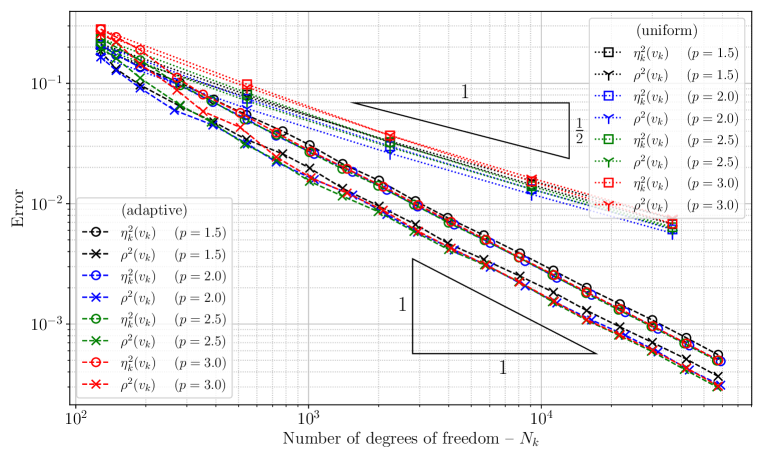
Figure 1: Plots of $\eta_{k}^{2}(v_{k})$ and $\rho^{2}(v_{k})$ for $p\in\{1.5,2,2.5,3\}$ and $v_{k}\coloneqq I_{h_{k}}^{\textit{av}}u_{k}^{\textit{cr}}\in\smash{\mathcal{S}^{1}_{D}(\mathcal{T}_{k})}$, using adaptive mesh refinement for $k=0,\dots,19$ and using uniform mesh refinement for $k=0,\dots,4$.

Appendix A Appendix

In this appendix, we give a proof of the inequalities (3.1).

Proposition A.1.

Let $\psi\colon\mathbb{R}_{\geq 0}\to\mathbb{R}_{\geq 0}$ be an $N$-function such that $\psi\in\Delta_{2}\cap\nabla_{2}$. Then, for every $v_{h}\in\mathcal{S}^{1,\textit{{cr}}}_{D}(\mathcal{T}_{h})$, $m\in\{0,1\}$, $a\geq 0$, and $T\in\mathcal{T}_{h}$, we have that

$$\fint_{T}{\psi_{a}(h_{T}^{m}|\nabla_{h}^{m}(v_{h}-{\color[rgb]{0,0,0}I_{h}^{\textit{av}}}v_{h})|)\,\textup{d}x}\leq c_{\textit{av}}\sum_{S\in\mathcal{S}_{h}(T)\setminus\Gamma_{N}}{\fint_{S}{\psi_{a}(|\llbracket{v_{h}}\rrbracket_{S}|)\,\textup{d}s}}\,,$$

where $c_{\textit{av}}>0$ depends only on $\Delta_{2}(\psi),\Delta_{2}(\psi^{*})>0$ and the chunkiness $\omega_{0}>0$.

Proof.

Owing to [9, Lemma A.2] together with [31, Lemma 12.1], there exists a constant $\overline{c}_{\textit{av}}>0$, depending only on the chunkiness $\omega_{0}>0$, such that

$$h_{T}^{m}\|\nabla_{h}^{m}(v_{h}-{\color[rgb]{0,0,0}I_{h}^{\textit{av}}}v_{h})\|_{L^{\infty}(T;\mathbb{R}^{d^{m}})}\leq\overline{c}_{\textit{av}}\sum_{\smash{S\in\mathcal{S}_{h}(T)\setminus\Gamma_{N}}}{\fint_{S}{|\llbracket{v_{h}}\rrbracket_{S}|\,\textup{d}s}}\,.$$ (A.1)

Therefore, using in (A.1) the $\Delta_{2}$-condition and convexity of $\psi_{a}\colon\mathbb{R}_{\geq 0}\to\mathbb{R}_{\geq 0}$, $a\geq 0$, in particular, Jensen’s inequality, and that $\sup_{h>0}{\sup_{T\in\mathcal{T}_{h}}{\textup{card}(\mathcal{S}_{h}(T)\setminus\Gamma_{N})}}\leq c_{\mathcal{T}}$, where $c_{\mathcal{T}}>0$ depends only on the chunkiness $\omega_{0}>0$, we find that

$$\fint_{T}{\psi_{a}(h_{T}^{m}|\nabla_{h}^{m}(v_{h}-{\color[rgb]{0,0,0}I_{h}^{\textit{av}}}v_{h})|)\,\textup{d}x} \leq\Delta_{2}(\psi_{a})^{\lceil\overline{c}_{\textit{av}}c_{\mathcal{T}}\rceil}\psi_{a}\bigg{(}\frac{1}{\textup{card}(\mathcal{S}_{h}(T)\setminus\Gamma_{N})}\sum_{S\in\mathcal{S}_{h}(T)\setminus\Gamma_{N}}{\fint_{S}{|\llbracket{v_{h}}\rrbracket_{S}|\,\textup{d}s}}\bigg{)}$$

$$\leq\Delta_{2}(\psi_{a})^{\lceil\overline{c}_{\textit{av}}c_{\mathcal{T}}\rceil}\frac{1}{\textup{card}(\mathcal{S}_{h}(T)\setminus\Gamma_{N})}\sum_{S\in\mathcal{S}_{h}(T)\setminus\Gamma_{N}}{\fint_{S}{\psi_{a}(|\llbracket{v_{h}}\rrbracket_{S}|)\,\textup{d}s}}\,.$$

Eventually, using that $\sup_{a\geq 0}{\Delta_{2}(\psi_{a})}<\infty$, cf. [23, Lemma 22], we conclude the assertion. ∎

Corollary A.2.

Let $\psi\colon\mathbb{R}_{\geq 0}\to\mathbb{R}_{\geq 0}$ be an $N$-function such that $\psi\in\Delta_{2}\cap\nabla_{2}$. Then, for every $v_{h}\in\mathcal{S}^{1,\textit{cr}}_{D}(\mathcal{T}_{h})$, $m\in\{0,1\}$, $a\geq 0$ and $T\in\mathcal{T}_{h}$, we have that

$$\fint_{T}{\psi_{a}(h_{T}^{m}|\nabla_{h}^{m}(v_{h}-{\color[rgb]{0,0,0}I_{h}^{\textit{av}}}v_{h})|)\,\textup{d}x} \leq c_{\textit{av}}\sum_{S\in\mathcal{S}_{h}(T)\setminus\Gamma_{N}}{\fint_{S}{\psi_{a}(h_{S}|\llbracket{\nabla_{h}v_{h}}\rrbracket_{S}|)\,\textup{d}s}}$$

$$\leq\tilde{c}_{\textit{av}}\fint_{\omega_{T}}{\psi_{a}(h_{T}|\nabla_{h}v_{h}|)\,\textup{d}x}\,,$$

where $\tilde{c}_{\textit{av}}>0$ depends only on $\Delta_{2}(\psi),\Delta_{2}(\psi^{*})>0$ and the chunkiness $\omega_{0}>0$.

Proof.

Follows from Proposition A.1, if we exploit that $\llbracket{v_{h}}\rrbracket_{S}=\llbracket{\nabla_{h}v_{h}}\rrbracket_{S}\cdot(\textup{id}_{\mathbb{R}^{d}}-x_{S})$ on $S$ for all $S\in\mathcal{S}_{h}$ and $v_{h}\in\mathcal{S}^{1,\textit{cr}}_{D}(\mathcal{T}_{h})$ and the discrete trace inequality [31, Lemma 12.8]. ∎

Acknowledgement. The author is grateful for the stimulating discussions with S. Bartels.

References

- [1] E. Acerbi and N. Fusco, Regularity for minimizers of nonquadratic functionals: the case , J. Math. Anal. Appl. 140 no. 1 (1989), 115–135.
- [2] P. R. Amestoy, I. S. Duff, J. Koster, and J.-Y. L’Excellent, A fully asynchronous multifrontal solver using distributed dynamic scheduling, SIAM Journal on Matrix Analysis and Applications 23 no. 1 (2001), 15–41.
- [3] S. Balay et al., and H. Zhang, PETSc Web page, https://www.mcs.anl.gov/petsc, 2019.
- [4] J. W. Barrett and W. B. Liu, Finite element approximation of the -Laplacian, Math. Comp. 61 no. 204 (1993), 523–537.
- [5] J. W. Barrett and W. B. Liu, Finite element approximation of degenerate quasilinear elliptic and parabolic problems, in Numerical analysis 1993 (Dundee, 1993), Pitman Res. Notes Math. Ser. 303, Longman Sci. Tech., Harlow, 1994, pp. 1–16.
- [6] J. W. Barrett and W. B. Liu, Quasi-norm error bounds for the finite element approximation of a non-Newtonian flow, Numer. Math. 68 no. 4 (1994), 437–456.
- [7] S. Bartels, Nonconforming discretizations of convex minimization problems and precise relations to mixed methods, Comput. Math. Appl. 93 (2021), 214–229. doi:10.1016/j.camwa.2021.04.014.
- [8] S. Bartels and A. Kaltenbach, Explicit and efficient error estimation for convex minimization problems, Math. Comp. (2023), accepted. doi:10.48550/ARXIV.2204.10745.
- [9] S. Bartels and A. Kaltenbach, Error analysis for a Crouzeix-Raviart approximation of the obstacle problem, 2023. doi:10.48550/ARXIV.2302.01646.
- [10] S. Bartels and M. Milicevic, Primal-dual gap estimators for a posteriori error analysis of nonsmooth minimization problems, ESAIM Math. Model. Numer. Anal. 54 (2020), 1635–1660. doi:10.1051/m2an/2019074.
- [11] L. Belenki, L. Diening, and C. Kreuzer, Optimality of an adaptive finite element method for the -Laplacian equation, IMA J. Numer. Anal. 32 no. 2 (2012), 484–510. doi:10.1093/imanum/drr016.
- [12] L. Berselli, L. Diening, and M. Růžička, Existence of strong solutions for incompressible fluids with shear dependent viscosities, Journal of Mathematical Fluid Mechanics 12 (2010), 101–132. doi:10.1007/s00021-008-0277-y.
- [13] L. C. Berselli and M. Růžička, Global regularity for systems with -structure depending on the symmetric gradient, Adv. Nonlinear Anal. 9 no. 1 (2020), 176–192. doi:10.1515/anona-2018-0090.
- [14] J. H. Bramble and S. R. Hilbert, Estimation of linear functionals on sobolev spaces with application to fourier transforms and spline interpolation, SIAM J. Numer. Anal. 7 no. 1 (1970), 112–124. doi:10.1137/0707006.
- [15] S. C. Brenner, Two-level additive schwarz preconditioners for nonconforming finite element methods, Mathematics of Computation 65 no. 215 (1996), 897–921.
- [16] S. C. Brenner, Forty years of the Crouzeix-Raviart element, Numer. Methods Partial Differential Equations 31 no. 2 (2015), 367–396. doi:10.1002/num.21892.
- [17] C. Carstensen, An adaptive mesh-refining algorithm allowing for an stable projection onto Courant finite element spaces, Constr. Approx. 20 no. 4 (2004), 549–564. doi:10.1007/s00365-003-0550-5.
- [18] C. Carstensen, W. Liu, and N. Yan, A posteriori FE error control for -Laplacian by gradient recovery in quasi-norm, Math. Comp. 75 no. 256 (2006), 1599–1616. doi:10.1090/S0025-5718-06-01819-9.
- [19] P. Ciarlet, The Finite Element Method for Elliptic Problems, Society for Industrial and Applied Mathematics, 2002. doi:10.1137/1.9780898719208.
- [20] M. Crouzeix and P.-A. Raviart, Conforming and nonconforming finite element methods for solving the stationary Stokes equations. I, Rev. Française Automat. Informat. Recherche Opérationnelle Sér. Rouge 7 no. R-3 (1973), 33–75.
- [21] B. Dacorogna, Direct methods in the calculus of variations, second ed., Applied Mathematical Sciences 78, Springer, New York, 2008.
- [22] L. Diening and F. Ettwein, Fractional estimates for non-differentiable elliptic systems with general growth, Forum Math. 20 no. 3 (2008), 523–556.
- [23] L. Diening and C. Kreuzer, Linear convergence of an adaptive finite element method for the -Laplacian equation, SIAM J. Numer. Anal. 46 no. 2 (2008), 614–638. doi:10.1137/070681508.
- [24] L. Diening, D. Kröner, M. Růžička, and I. Toulopoulos, A Local Discontinuous Galerkin approximation for systems with -structure, IMA J. Num. Anal. 34 no. 4 (2014), 1447–1488. doi:doi: 10.1093/imanum/drt040.
- [25] L. Diening and M. Růžička, Interpolation operators in Orlicz-Sobolev spaces, Numer. Math. 107 no. 1 (2007), 107–129. doi:10.1007/s00211-007-0079-9.
- [26] W. Dörfler, A convergent adaptive algorithm for Poisson’s equation, SIAM J. Numer. Anal. 33 no. 3 (1996), 1106–1124. doi:10.1137/0733054.
- [27] C. Ebmeyer, Global regularity in nikolskij spaces for elliptic equations with p-structure on polyhedral domains, Nonlinear Analysis 63 no. 6-7 (2005), e1–e9.
- [28] C. Ebmeyer and W. B. Liu, Quasi-norm interpolation error estimates for finite element approximations of problems with –structure, Numer. Math. 100 (2005), 233–258.
- [29] C. Ebmeyer, W. Liu, and M. Steinhauer, Global regularity in fractional order Sobolev spaces for the -Laplace equation on polyhedral domains, Z. Anal. Anwendungen 24 no. 2 (2005), 353–374.
- [30] I. Ekeland and R. Témam, Convex analysis and variational problems, english ed., Classics in Applied Mathematics 28, Society for Industrial and Applied Mathematics (SIAM), Philadelphia, PA, 1999, doi:10.1137/1.9781611971088.
- [31] A. Ern and J. L. Guermond, Finite Elements I: Approximation and Interpolation, Texts in Applied Mathematics no. 1, Springer International Publishing, 2021. doi:10.1007/978-3-030-56341-7.
- [32] E. Giusti, Direct methods in the calculus of variations, World Scientific Publishing Co. Inc., River Edge, NJ, 2003.
- [33] C. Helanow and J. Ahlkrona, Stabilized equal low-order finite elements in ice sheet modeling—accuracy and robustness, Comput. Geosci. 22 no. 4 (2018), 951–974. doi:10.1007/s10596-017-9713-5.
- [34] J. D. Hunter, Matplotlib: A 2d graphics environment, Computing in Science & Engineering 9 no. 3 (2007), 90–95. doi:10.1109/MCSE.2007.55.
- [35] A. Kaltenbach and M. Růžička, Convergence analysis of a Local Discontinuous Galerkin approximation for nonlinear systems with Orlicz-structure, 2022. doi:10.48550/arXiv.2204.09984
- [36] A. Kaltenbach and M. Zeinhofer, The Deep Ritz Method for Parametric -Dirichlet Problems, 2022. doi:10.48550/arXiv.2207.01894.
- [37] D. J. Liu, A. Q. Li, and Z. R. Chen, Nonconforming FEMs for the -Laplace problem, Adv. Appl. Math. Mech. 10 no. 6 (2018), 1365–1383.doi:10.4208/aamm.
- [38] W. Liu and N. Yan, Quasi-norm a priori and a posteriori error estimates for the nonconforming approximation of -Laplacian, Numer. Math. 89 no. 2 (2001), 341–378. doi:10.1007/PL00005470.
- [39] W. Liu and N. Yan, Quasi-norm local error estimators for -Laplacian, SIAM J. Numer. Anal. 39 no. 1 (2001), 100–127. doi:10.1137/S0036142999351613.
- [40] W. B. Liu, Degenerate quasilinear elliptic equations arising from bimaterial problems in elastic-plastic mechanics, Nonlinear Anal. 35 no. 4, Ser. A: Theory Methods (1999), 517–529. doi:10.1016/S0362-546X(98)00014-5.
- [41] A. Logg and G. N. Wells, Dolfin: Automated finite element computing, ACM Transactions on Mathematical Software 37 no. 2 (2010). doi:10.1145/1731022.1731030.
- [42] J. Málek, J. Nečas, M. Rokyta, and M. Růžička, Weak and measure-valued solutions to evolutionary PDEs, Applied Mathematics and Mathematical Computation 13, Chapman & Hall, London, 1996. doi:10.1007/978-1-4899-6824-1.
- [43] T. Malkmus, M. Růžička, S. Eckstein, and I. Toulopoulos, Generalizations of SIP methods to systems with -structure, IMA J. Numer. Anal. 38 no. 3 (2018), 1420–1451. doi:10.1093/imanum/drx040.
- [44] P. Oswald, On the robustness of the bpx-preconditioner with respect to jumps in the coefficients, Math. Comp. 68 no. 226 (1999), 633–650.
- [45] C. Padra, A posteriori error estimators for nonconforming approximation of some quasi-newtonian flows, SIAM J. Numer. Anal. 34 no. 4 (1997), 1600–1615. doi:10.1137/S0036142994278322.
- [46] P.-A. Raviart and J. M. Thomas, A mixed finite element method for 2nd order elliptic problems, in Mathematical aspects of finite element methods (Proc. Conf., Consiglio Naz. delle Ricerche (C.N.R.), Rome, 1975), 1977, pp. 292–315. Lecture Notes in Math., Vol. 606.
- [47] M. Růžička and L. Diening, Non–Newtonian fluids and function spaces, in Nonlinear Analysis, Function Spaces and Applications, Proceedings of NAFSA 2006 Prague, 8, 2007, pp. 95–144.
- [48] L. Scott and S. Zhang, Finite element interpolation of nonsmooth functions satisfying boundary conditions, Math. Comp. 54 (1990), 483–493. doi:10.1090/S0025-5718-1990-1011446-7.
- [49] R. Verfürth, A posteriori error estimates for nonlinear problems, Math. Comp. (1994), 445–475.
- [50] E. Zeidler, Nonlinear functional analysis and its applications. II/B Nonlinear monotone operators, Springer-Verlag, New York, 1990. doi:10.1007/978-1-4612-0985-0.