Adversarial permutation invariant training
for universal sound separation

Abstract

Universal sound separation consists of separating mixes with arbitrary sounds of different types, and permutation invariant training (PIT) is used to train source agnostic models that do so. In this work, we complement PIT with adversarial losses but find it challenging with the standard formulation used in speech source separation. We overcome this challenge with a novel $I$-replacement context-based adversarial loss, and by training with multiple discriminators. Our experiments show that by simply improving the loss (keeping the same model and dataset) we obtain a non-negligible improvement of 1.4 dB $\text{SI-SNR}_{\text{I}}$ in the reverberant FUSS dataset. We also find adversarial PIT to be effective at reducing spectral holes, ubiquitous in mask-based separation models, which highlights the potential relevance of adversarial losses for source separation.

Index Terms—  Adversarial, PIT, universal source separation.

1 Introduction

Audio source separation consists of separating the sources present in an audio mix, as in music source separation (separating vocals, bass, and drums from a music mix [1, 2, 3]) or speech source separation (separating various speakers talking simultaneously [4, 5, 6]). Recently, universal sound separation was proposed [7]. It consists of building source agnostic models that are not constrained to a specific domain (like music or speech) and can separate any source given an arbitrary mix. Permutation invariant training (PIT) [8] is used for training universal source separation models based on deep learning [7, 9, 10].

We consider mixes $m$ of length $L$ with $K^{\prime}$ arbitrary sources $\mathbf{{s}}$ as follows: $m=\sum_{k=1}^{K^{\prime}}s_{k}$, out of which the separator model $f_{\mathbf{\theta}}$ predicts $K$ sources $\mathbf{\hat{s}}=f_{\mathbf{\theta}}(m)$. PIT optimizes the learnable parameters $\mathbf{\theta}$ of $f_{\mathbf{\theta}}$ by minimizing the following permutation invariant loss:

$$\mathcal{L}_{\text{PIT}}=\min_{\mathbf{P}}\sum_{k=1}^{K}\mathcal{L}\left(s_{k},\left[\mathbf{P}{\hat{\mathbf{s}}}\right]_{k}\right),$$ (1)

where we consider all permutation matrices $\mathbf{P}$, $\mathbf{P}^{*}$ is the optimal permutation matrix minimizing Eq. 1, and $\mathcal{L}$ can be any regression loss. Since $f_{\mathbf{\theta}}$ outputs $K$ sources, in case a mix contains $K^{\prime}<K$ sources, we set the target ${s}_{k}=0$ for $k>K^{\prime}$. Note that a permutation invariant loss is required to build source agnostic models, because the outputs of $f_{\mathbf{\theta}}$ can be any source and in any order. As such, the model must not focus on predicting one source type per output, and any possible permutation of output sources must be equally correct [7, 8]. A common loss $\mathcal{L}$ for universal sound separation is the $\tau$-thresholded logarithmic mean squared error [7, 9], which is unbounded when ${s}_{k}=0$. In that case, since $m\neq 0$, one can use a different $\mathcal{L}$ based on thresholding with respect to the mixture [9]:

$$\mathcal{L}(s_{k},\hat{s}_{k})=\begin{cases}10\log_{10}\left(\|\hat{{s}_{k}}\|^{2}+\tau\|m\|^{2}\right)&\text{if }s_{k}=0\\ 10\log_{10}\left(\|{s}_{k}-\hat{{s}}_{k}\|^{2}+\tau\|{s}_{k}\|^{2}\right)&\text{otherwise.}\end{cases}$$ (2)

Previous works on (two speaker)	Discriminator type and input	Multiple $D$?	Input to $D$	With $\mathcal{L}_{\text{PIT}}$?	Adversarial
speech source separation	(Type $\rightarrow$ Input: real / fake)		(domain)	(+$\mathcal{L}_{\text{PIT}}$ domain)	loss
CBLDNN [11]	$D_{\text{ctx},I=0}^{\text{STFT}}$  $\rightarrow$  $[m,{s_{1}},{s_{2}}]$ / $[m,\hat{s}_{1},\hat{s}_{2}]$ ($m$-conditioned)	No	$|$STFT$|$	Yes, $|$STFT$|$	LSGAN
SSGAN-PIT [12]: variant (i)	$D_{\text{ctx},I=0}^{\text{STFT}}$  $\rightarrow$  $[m,{s_{1}},{s_{2}}]$ / $[m,\hat{s}_{1},\hat{s}_{2}]$ ($m$-conditioned)	No	$|$STFT$|$	Yes, $|$STFT$|$	LSGAN
SSGAN-PIT [12]: variant (ii)	$D_{\text{ctx},I=0}^{\text{STFT}}$  $\rightarrow$  $[{s_{1}},{s_{2}}]$ / $[\hat{s}_{1},\hat{s}_{2}]$	No	$|$STFT$|$	Yes, $|$STFT$|$	LSGAN
SSGAN-PIT [12]: variant (iii)	$D_{\text{inst}}^{\text{STFT}}$  $\rightarrow$  $[{s}_{1}]$ / $[\hat{s}_{1}]$  and  $[{s}_{2}]$ / $[\hat{s}_{2}]$	No	$|$STFT$|$	Yes, $|$STFT$|$	LSGAN
Furcax [13]	$D_{\text{ctx},I=0}^{\text{wave}}$  $\rightarrow$  $[{s_{1}},{s_{2}}]$ / $[\hat{s}_{1},\hat{s}_{2}]$	No	Waveform	Yes, waveform	LSGAN
Conv-TasSAN [14]	Metric predictor  $\rightarrow$  $[{s_{1}},{s_{2}},{s_{1}},{s_{2}}]$ / $[\hat{s}_{1},\hat{s}_{2},{s_{1}},{s_{2}}]$	No	Waveform	Yes, waveform	MetricGAN
Our source agnostic method for universal sound separation	Any above except “metric predictor”; with more than	Yes, for better quality	Any above, plus masks
	two input sources; using ${D}_{\text{ctx,}I>0}$ with $I$-replacement;			Optional	Hinge loss
	and with source agnostic discriminators

Table 1: Summary of differences between our work (bottom) and previous adversarial PIT works for speech source separation (top).

In this work, we complement PIT with adversarial losses for universal sound separation. A number of speech source separation works also complemented PIT with adversarial losses [11, 12, 13, 14]. Yet, we find that the adversarial PIT formulation used in speech separation does not perform well for universal source separation (sections 3 and 4). To improve upon that, in section 2 we extend speech separation works with: a novel $I$-replacement context-based adversarial loss, by combining multiple discriminators, and generalize adversarial PIT such that it works for universal sound separation (with source agnostic discriminators dealing with more than two sources). Table 1 outlines how our approach compares with speech separation works.

2 Adversarial PIT

Adversarial training, in the context of source separation, consists of simultaneously training two models: $f_{\theta}$ producing plausible separations $\mathbf{\hat{s}}$, and one (or multiple) discriminator(s) $D$ assessing if separations $\mathbf{\hat{s}}$ are produced by $f_{\theta}$ (fake) or are ground-truth separations $\mathbf{{s}}$ (real). Under this setup, the goal of $f_{\theta}$ is to estimate (fake) separations that are as close as possible to the (real) ones from the dataset, such that $D$ misclassifies $\mathbf{\hat{s}}$ as $\mathbf{{s}}$ [15, 16]. We propose combining variations of an instance-based discriminator $D_{\text{inst}}$ with a novel $I$-replacement context-based discriminator $D_{\text{ctx},I}$. Each $D$ has a different role and is applicable to various domains: waveforms, magnitude STFTs, or masks. Without loss of generality, we present $D_{\text{inst}}$ and $D_{\text{ctx},I}$ in the waveform domain and then show how to combine multiple discriminators operating at various domains to train $f_{\theta}$.

Instance-based adversarial loss — The role of $D_{\text{inst}}$ is to provide adversarial cues on the realness of the separated sources without context. That is, $D_{\text{inst}}$ assesses the realness of each source individually:

$$[s_{1}]\ /\ [\hat{s}_{1}]\ \ldots\ [s_{K}]\ /\ [\hat{s}_{K}].$$

Throughout the paper, we use brackets $[~{}]$ to denote the $D$’s input and left / right for real / fake separations (not division). Hence, individual real / fake separations (instances) are input to $D_{\text{inst}}$, which learns to classify them as real / fake (Fig. 1). $D_{\text{inst}}$ is trained to maximize

$$\mathcal{L}_{\text{inst}}=\frac{1}{K}\sum_{k=1}^{K}(\mathcal{L}_{\text{inst}}^{\text{real},k}+\mathcal{L}_{\text{inst}}^{\text{fake},k}),$$

where $\mathcal{L}_{\text{inst}}^{\text{real},k}$ and $\mathcal{L}_{\text{inst}}^{\text{fake},k}$ correspond to the hinge loss [17]:

$$\mathcal{L}_{\text{inst}}^{\text{real},k} =\min\left(0,-1+D_{\text{inst}}(s_{k})\right),$$

$$\mathcal{L}_{\text{inst}}^{\text{fake},k} =\min\left(0,-1-D_{\text{inst}}(\hat{s}_{k})\right).$$

Previous works also explored using $D_{\text{inst}}$. However, they used source specific setups where each $D_{\text{inst}}$ was specialized in a source type, e.g., for music source separation each $D_{\text{inst}}$ was specialized in bass, drums, and vocals [1, 18], or for speech source separation $D_{\text{inst}}$ was specialized in speech [19, 12]. Yet, each $D_{\text{inst}}$ for universal sound separation is not specialized in any source type (are source agnostic) and assesses the realness of any audio, regardless of its source type.

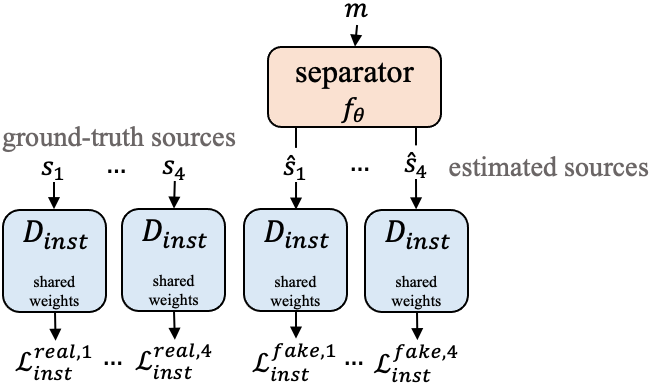
Fig. 1: Instance-based adversarial loss ($K=4$).

$I$-replacement context-based adversarial loss — The role of $D_{\text{ctx},I}$ is to provide adversarial cues on the realness of the separated sources considering all the sources in the mix (the context):

$$[s_{1},\dots,s_{K}]\ /\ [\bar{s}_{1},\dots,\bar{s}_{K}].$$

Here, all the separations are input jointly to provide context to $D_{\text{ctx},I}$, which learns to classify them as real / fake. $D_{\text{ctx},I}$ can also be conditioned on the input mix $m$:

$$[m,s_{1},\dots,s_{K}]\ /\ [m,\bar{s}_{1},\dots,\bar{s}_{K}].$$

Fake inputs contain entries $\bar{s}_{k}$, obtained by randomly getting $I<K$ source indices without replacement $\Lambda_{I}\subset\{1,\dots,K\}$, and substituting the selected estimated sources $\hat{s}^{*}_{k}$ with their ground-truth $s_{k}$:

$$\bar{s}_{k}=\begin{cases}s_{k}&\text{if }k\in\Lambda_{I},\\ \hat{s}^{*}_{k}&\text{otherwise},\end{cases}$$ (3)

where $\hat{s}^{*}_{k}=[\mathbf{P}^{*}\mathbf{\hat{s}}]_{k}$ and $\mathbf{P}^{*}$ is the optimal permutation matrix minimizing Eq. 1 with $\mathcal{L}$ as in Eq. 2. Note that finding the right permutation $\mathbf{P}^{*}$ is important to replace the selected source $\hat{s}^{*}_{k}$ with its corresponding ground-truth ${s}_{k}$, because the (source agnostic) estimations do not necessarily match the order of the ground-truth (see Fig. 2). Also, note that the $I=0$ case corresponds to the standard context-based adversarial loss used for speech source separation (without $I$-replacement, see Table 1). Thus, our work generalizes adversarial PIT for universal sound separation by proposing a novel $I$-replacing schema that explicitly uses the ground-truth to guide the adversarial loss. $D_{\text{ctx},I}$ is trained to maximize

$$\mathcal{L}_{\text{ctx},I}=\mathcal{L}^{\text{real}}_{\text{ctx},I}+\mathcal{L}^{\text{fake}}_{\text{ctx},I},$$

where we again use the hinge loss [17]:

$$\mathcal{L}^{\text{real}}_{\text{ctx},I} =\min(0,-1+D_{\text{ctx},I}(s_{1},\dots,s_{K})),$$

$$\mathcal{L}^{\text{fake}}_{\text{ctx},I} =\min(0,-1-D_{\text{ctx},I}(\bar{s}_{1},\dots,\bar{s}_{K})).$$

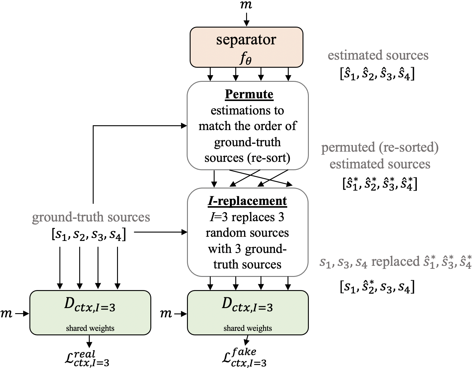
Fig. 2: $I$-replacement context-based adversarial loss ($I=3$, $K=4$).

Training with multiple discriminators — We have just presented $D_{\text{inst}}$ and $D_{\text{ctx},I}$ in the waveform domain: $D^{\text{wave}}_{\text{inst}}$ and $D^{\text{wave}}_{\text{ctx},I}$. Next, we introduce them in the magnitude STFT ($D^{\text{STFT}}_{\text{inst}},D^{\text{STFT}}_{\text{ctx},I}$) and mask ($D^{\text{mask}}_{\text{inst}},D^{\text{mask}}_{\text{ctx},I}$) domains, and explain how to combine them. The short-time Fourier transform (STFT) of a mix $m$ is defined as $M=\text{STFT}(m)$. The magnitude STFT is then obtained by taking the absolute value of $M$ in the complex domain, namely $|M|$. Similarly, we denote as $|S_{k}|$ and $|\hat{S}_{k}|$ the magnitude STFTs of the target and the estimated sources, respectively. Ratio masks

$$R_{k}=\frac{|S_{k}|}{\sum_{k=1}^{K}|S_{k}|}$$

are used to filter sources out from the mix by computing $S_{k}=M\odot R_{k}$, where $\odot$ denotes the element-wise product. Following the same notation as above, the input to the instance-based $D_{\text{inst}}^{\text{STFT}}$ and $D_{\text{inst}}^{\text{mask}}$ is

$$\begin{array}[]{cc}D^{\text{STFT}}_{\text{inst}}:&\left[|S_{1}|\right]\ /\ [|\hat{S}_{1}|]\ \ldots\ \left[|S_{K}|\right]\ /\ [|\hat{S}_{K}|],\\ D^{\text{mask}}_{\text{inst}}:&[R_{1}]\ /\ [\hat{R}_{1}]\ \ldots\ [R_{K}]\ /\ [\hat{R}_{K}],\end{array}\vspace{-1mm}$$

and for the context-based $D_{\text{ctx,}I}^{\text{STFT}}$ and $D_{\text{ctx,}I}^{\text{mask}}$ (conditioned on $m$) is

$$\begin{array}[]{cc}D^{\text{STFT}}_{\text{ctx},I}:&[|M|,|S_{1}|,\dots,|S_{K}|]\ /\ [|M|,|\bar{S}_{1}|,\dots,|\bar{S}_{K}|],\\ D^{\text{mask}}_{\text{ctx},I}:&[|M|,R_{1},\dots,R_{K}]\ /\ [|M|,\bar{R}_{1},\dots,\bar{R}_{K}],\end{array}$$

where $|\bar{S}_{k}|$ and $\bar{R}_{k}$ entries follow the same $I$-replacement procedure as in Eq. 3. Here, for $D_{\text{ctx},I}^{\text{STFT}}$ and $D_{\text{ctx},I}^{\text{mask}}$, the optimal permutation matrix $\mathbf{P}^{*}$ required for re-sorting the fake examples is computed considering the L1-loss between magnitude STFTs or masks. The motivation behind combining multiple discriminators is to facilitate a richer set of adversarial loss cues to train $f_{\theta}$ [18, 20, 21], such that both $D_{\text{inst}}$ and $D_{\text{ctx},I}$ can provide different perspectives with respect to the same signal in various domains: waveform, magnitude STFT, and mask. Hence, in addition to train each $D$ alone, one can train multiple combinations, e.g., $D^{\text{wave}}_{\text{inst}}+D^{\text{wave}}_{\text{ctx},I}$, $D^{\text{wave}}_{\text{ctx},I}+D^{\text{STFT}}_{\text{ctx},I}+D^{\text{mask}}_{\text{ctx},I}$, or any combination of the discriminators above. However, the more discriminators used, the more computationally expensive it is to run the loss, and the longer it takes to train $f_{\mathbf{\theta}}$ (but does not affect inference time). To the best of our knowledge, training with multiple discriminators has never been considered for source separation before.

Separator loss — In adversarial training, $f_{\theta}$ is trained such that its (fake) separations $\mathbf{\hat{s}}$ are misclassified by the discriminator(s) as ground-truth ones $\mathbf{{s}}$ (real). To do so, during every adversarial training step, we first update the discriminator(s) (without updating $f_{\theta}$) based on $\mathcal{L}_{\text{inst}}$, $\mathcal{L}_{\text{ctx},I}$, or any combination of the losses above. Then, $\mathcal{L}_{\text{sep}}$ is minimized to train $f_{\theta}$ without updating the discriminator(s). For example, when using $D^{\text{wave}}_{\text{inst}}$ (with $D^{\text{wave}}_{\text{inst}}$ frozen) we minimize

$$\mathcal{L}_{\text{sep}}=-\frac{1}{K}\sum_{k=1}^{K}D^{\text{wave}}_{\text{inst}}(\hat{s}_{k}),$$

when using $D^{\text{STFT}}_{\text{ctx},I}$ (with $D^{\text{STFT}}_{\text{ctx},I}$ frozen) we minimize

$$\mathcal{L}_{\text{sep}}=-D^{\text{STFT}}_{\text{ctx},I}(|\bar{S}_{1}|,\dots,|\bar{S}_{K}|),$$

or when using $D^{\text{STFT}}_{\text{inst}}$ and $D^{\text{STFT}}_{\text{ctx},I}$ conditioned on $m$ (with $D^{\text{STFT}}_{\text{inst}}$ and $D^{\text{STFT}}_{\text{ctx},I}$ frozen) we minimize

$$\mathcal{L}_{\text{sep}}=-\frac{1}{K}\sum_{k=1}^{K} D^{\text{STFT}}_{\text{inst}}(|\hat{S}_{k}|)-D^{\text{STFT}}_{\text{ctx},I}(|M|,|\bar{S}_{1}|,\dots,|\bar{S}_{K}|).$$

Again, note that we use the hinge loss [17]. While we are not presenting all possible loss combinations for brevity, from the above examples one can infer all the combinations we experiment with in section 4. Finally, we can also add an $\mathcal{L}_{\text{PIT}}$ term (as in Eqs. 1 and  2) to adversarial PIT: $\mathcal{L}_{\text{sep}}+\lambda\mathcal{L}_{\text{PIT}}$, where $\lambda$ scales $\mathcal{L}_{\text{PIT}}$ such that it is of the same magnitude as $\mathcal{L}_{\text{sep}}$ [22]. All previous adversarial PIT works for speech source separation used $\mathcal{L}_{\text{sep}}+\lambda\mathcal{L}_{\text{PIT}}$ (Table 1). Yet, in section 4 we show that our adversarial training setup allows dropping $\mathcal{L}_{\text{PIT}}$ while still obtaining competitive results, possibly because of the strong cues provided by $D_{\text{ctx},I}$ (with $I$-replacement) and the multiple discriminators. To the best of our knowledge, we are the first to report results similar to $\mathcal{L}_{\text{PIT}}$ with a purely adversarial setup (cf. [12]).

3 EXPERIMENTAL SETUP

Dataset, evaluation metrics, and baseline — We use the reverberant FUSS dataset, a common benchmark for universal sound separation with 20 k / 1 k / 1 k (train / val / test) mixes of 10 s with one to four sources [9, 23, 24]. Metrics rely on the scale-invariant SNR [9]:

$$\text{SI-SNR}(s_{k},\hat{{s}}_{k}^{*})=10\log_{10}\frac{\|{\alpha s_{k}}\|^{2}+\epsilon}{\|\alpha s_{k}-\hat{{s}}_{k}^{*}\|^{2}+\epsilon},$$

where $\alpha=\frac{{s_{k}}^{T}\hat{s}_{k}^{*}+\epsilon}{\|s_{k}\|^{2}+\epsilon}$, $\epsilon=10^{-5}$, and $\hat{s}^{*}_{k}=[\mathbf{P}^{*}\mathbf{\hat{s}}]_{k}$ with $\mathbf{P}^{*}$ being the optimal source-permutation matrix maximizing SI-SNR. Further, to account for inactive sources, estimate-target pairs that have silent target sources are discarded [10]. For mixes with one source, we compute $\text{SI-SNR}_{\text{S}}=\text{SI-SNR}(s_{k},\hat{s}^{*}_{k})$, which is equivalent to $\text{SI-SNR}(m,\hat{s}^{*}_{k})$ since with one-source mixes the goal is to bypass the mix (the S sub-index stands for single-source). For mixes with two to four sources, we report the average across sources of the $\text{SI-SNR}_{\text{I}}=\text{SI-SNR}(s_{k},\hat{s}^{*}_{k})-\text{SI-SNR}(s_{k},m)$ (the I sub-index stands for improvement). Note that we are using the standard SI-SNR formulation as in [10] instead of the alternative (less common) SI-SNR in [9, 25], and that we use the reverberant FUSS dataset as in [9, 26] instead of its dry counterpart [25, 10] because it is more realistic. As such, the results in [9, 10, 25] are not comparable with ours because they either use a different SI-SNR formulation or a different dataset. To compare our work against a meaningful state-of-the-art baseline we use the DCASE model, a TDCN++ predicting STFT masks [26]. It is trained on the reverberant FUSS dataset, and we evaluate it with the metrics based on the standard SI-SNR. Finally, we report $\text{SI-SNR}_{\text{S}}$ for consistency [9, 10], but $\text{SI-SNR}_{\text{I}}$ scores are more relevant for comparing models since most $\text{SI-SNR}_{\text{S}}$ scores are already very close to the upper-bound of 39.9 dB (see Table 3).

Separator — The mix $m$ of length $L=160000$ (10 s at 16 kHz) is mapped to the STFT domain $M$, with windows of 32 ms and 25% overlap (256 frequency bins and 1250 frames). From $M$ we obtain its magnitude STFT $|M|$, that is input to a U-Net $g_{\theta}$ that predicts a ratio mask $\hat{R}_{k}$. The mask is obtained using a softmax layer $\sigma$ across the source dimension $k$: $\mathbf{\hat{R}}=\sigma(g_{\theta}(|M|))$, such that $\sum_{k}|{\hat{S}_{k}}|=|M|$. Then, we filter the estimated STFTs out of the mix with ${\hat{S}_{k}}={M\odot\hat{R}_{k}}$, and use the inverse STFT to get the waveform estimates: $\mathbf{\hat{s}}=f_{\theta}(m)=\text{iSTFT}(\mathbf{\hat{S}})$. Hence, our separator can be trained in the waveform domain (with $\mathcal{L}_{\text{PIT}}$, $D_{\text{ctx},I}^{\text{wave}}$, $D^{\text{wave}}_{\text{inst}}$), in the magnitude STFT domain (with $D_{\text{ctx},I}^{\text{STFT}}$, $D^{\text{STFT}}_{\text{inst}}$), and/or in the mask domain (with $D_{\text{ctx},I}^{\text{mask}}$, $D^{\text{mask}}_{\text{inst}}$). Our U-Net $g_{\theta}$ (of 46.9 M parameters) consists of an encoder, a bottleneck, and a decoder whose inputs include the corresponding encoder’s block outputs [27, 28]. The encoder is built of 4 ResNet blocks, each followed by a downsampler that is a 1D-CNN (kernel size=3, stride=2). The number of channels across encoder blocks is [256, 512, 512, 512]. The bottleneck consists of a ResNet block, self-attention, and another ResNet block (with all layers having 512 channels). The decoder block is built of 4 ResNet blocks, reversing the structure of the encoder, with upsamplers in place of downsamplers, reversing the number of channels of the encoder. The upsamplers perform linear interpolation followed by a 1D-CNN (kernel size=3, stride=1). A final linear layer adapts the output to predict the expected number of sources ($K=4$).

Discriminators — Each $D$ is of around 900 k parameters, are fully convolutional, and output one scalar. $D^{\text{wave}}_{\text{inst}}$ and $D^{\text{wave}}_{\text{ctx},I}$ rely on a similar model: 4 1D-CNN layers (kernel size=4, stride=3), interleaved by LeakyReLUs, with the following number of channels: [$C$, 128, 256, 256, 512], where $C=1$ for $D^{\text{wave}}_{\text{inst}}$, and $C=5$ or $4$ for $D^{\text{wave}}_{\text{ctx},I}$, depending if it is $m$-conditioned or not. Then, the 512 channels are projected to 1 with a 1D-CNN (kernel size=4, stride=1), and the final linear layer maps the remaining temporal dimension into a scalar. $D^{\text{STFT}}_{\text{inst}}$, $D^{\text{STFT}}_{\text{ctx},I}$, $D^{\text{mask}}_{\text{inst}}$, and $D^{\text{mask}}_{\text{ctx},I}$ are similar to $D^{\text{wave}}_{\text{inst}}$ and $D^{\text{wave}}_{\text{ctx},I}$, with the difference that 1D-CNNs are 2D (kernel size=4$\times$4, stride=3$\times$3) and the number of channels is [$C$, 64, 128, 128, 256].

Training and evaluation setup — Models are trained until convergence (around 500 k iterations) using the Adam optimizer, and the best model on the validation set is selected for evaluation. For training, we adjust the learning rate $\{10^{-5},10^{-4},10^{-3}\}$ and batch size $\{16,32,64,96,128\}$ such that all experiments, including ablations and baselines, get the best possible results. Finally, we use a mixture-consistency projection [29] at inference time (not during training) because it systematically improved our $\text{SI-SNR}_{\text{S}}$ without degrading $\text{SI-SNR}_{\text{I}}$. Our best model was trained for a month with 4 V100 GPUs with a learning rate of $10^{-4}$ and a batch size of 128.

4 EXPERIMENTS AND DISCUSSION

First, in Table 3, we study various $D_{\text{ctx},I}$ configurations. We observe that the standard adversarial PIT ($I=0$, as in speech source separation) consistently obtains the worst results for universal sound separation. In contrast, the models trained with $I$-replacement ($I>0$) consistently obtain the best results. We hypothesize that with $I=0$ $f_{\theta}$ does not separate much. Instead, it tends to approximate the naive solution of bypassing the mix. We can see this with the $\text{SI-SNR}_{\text{S}}$ scores, which tend to be closer (if not the same) to the $\text{SI-SNR}_{\text{S}}$ of the lower and upper bounds in Table 3. Overall, we note that the $I$-replacement context-based adversarial loss seems key to generalize adversarial PIT for universal sound separation, where multiple heterogeneous sources are separated. This contrasts with adversarial PIT works for speech source separation, where two similar sources are separated. We argue that the universal sound separation case is more challenging, as speech separation discriminators can judge the realness of separations based on speech cues, but discriminators for universal sound separation cannot as sources can be of any kind. We hypothesize that the effectiveness of ${D}_{\text{ctx,}I>0}$ can be attributed to:

• Replacing ${\hat{s}^{*}}_{k}$ with ${{s}}_{k}$ explicitly guides the adversarial loss to perform source separation. Note that $D_{\text{ctx},I=0}$ (and $D_{\text{inst}}$) focuses on assessing the realness of its input. Under this setup, a naive solution is to always bypass the mix, which looks as real as one-source mixes where the goal is to bypass the mix. To avoid this naive solution, some guidance like the $I$-replacement is required.

• It is more difficult for ${D}_{\text{ctx,}I>0}$ to distinguish between real and fake separations, because fake ones contain replacements. Consequently, such replacements help defining a non-trivial task for the discriminator that results in a better adversarial loss to train $f_{\theta}$.

$m$	$D_{\text{ctx},I}^{\text{STFT}}$	SI-SNR	$D_{\text{ctx},I}^{\text{mask}}$	SI-SNR	$D_{\text{ctx},I}^{\text{wave}}$	SI-SNR
Yes	$I$$=$$0$	4.9 / 35.7	$I$$=$$0$	5.9 / 35.8	$I$$=$$0$	8.5 / 39.9
Yes	$I$$=$$1$	11.0 / 33.2	$I$$=$$1$	9.3 / 33.6	$I$$=$$1$	11.3 / 35.5
Yes	$I$$=$$2$	10.7 / 33.1	$I$$=$$2$	9.6 / 34.3	$I$$=$$2$	11.9 / 36.3
Yes	$I$$=$$3$	11.7 / 33.4	$I$$=$$3$	8.6 / 32.6	$I$$=$$3$	12.1 / 35.9
No	$I$$=$$0$	5.7 / 35.0	$I$$=$$0$	3.8 / 36.8	$I$$=$$0$	8.5 / 39.9
No	$I$$=$$1$	9.9 / 32.8	$I$$=$$1$	6.7 / 34.1	$I$$=$$1$	10.3 / 37.6
No	$I$$=$$2$	10.4 / 32.0	$I$$=$$2$	9.0 / 33.6	$I$$=$$2$	11.0 / 36.0
No	$I$$=$$3$	10.2 / 31.0	$I$$=$$3$	9.7 / 33.5	$I$$=$$3$	11.4 / 35.3

Table 2: Study of various $D_{\text{ctx},I}$ configurations. $m$ column: $D_{\text{ctx},I}$ is $m$-conditioned or not. SI-SNR column: $\text{SI-SNR}_{\text{I}}$ / $\text{SI-SNR}_{\text{S}}$ in dB.

$\mathcal{L}_{\text{ctx},I}^{\text{STFT}}$	$\mathcal{L}_{\text{ctx},I}^{\text{wave}}$	$\mathcal{L}_{\text{ctx},I}^{\text{mask}}$	$\mathcal{L}^{\text{STFT}}_{\text{inst}}$	$\mathcal{L}^{\text{wave}}_{\text{inst}}$	$\mathcal{L}^{\text{mask}}_{\text{inst}}$	$\mathcal{L}_{\text{PIT}}$	SI-SNR ($\uparrow$)
✓	✓	✓	✓	✓	✓	✓	13.5 / 37.2
✓	✓	✓	✓	✓	✓	-	12.9 / 36.7
✓	✓	✓	-	-	-	-	12.5 / 37.3
✓	✓	-	✓	✓	-	✓	13.8 / 35.3
✓	✓	-	✓	✓	-	-	12.0 / 38.3
✓	✓	-	-	-	-	-	11.6 / 35.3
✓	-	-	-	-	-	-	11.7 / 33.4
-	✓	-	-	-	-	-	12.1 / 35.9
-	-	✓	-	-	-	-	8.6 / 32.6
-	-	-	✓	-	-	-	8.2 / 27.0
-	-	-	-	✓	-	-	4.7 / 27.7
-	-	-	-	-	✓	-	4.5 / 36.8
-	-	-	-	-	-	✓	12.4 / 37.4
DCASE PIT baseline [26]							12.8 / 37.5
Lower-bound: return the input mix $m$							0.0 / 39.9
Upper-bound: ideal ratio STFT masks [30]							25.3 / 39.9

Table 3: Comparison of adversarial PIT variants and baselines. SI-SNR column: $\text{SI-SNR}_{\text{I}}$ / $\text{SI-SNR}_{\text{S}}$ in dB. All $D_{\text{ctx},I}$ above are $m$-conditioned with $I$$=$$3$, since it outperforms other setups (Table 3). All adversarial PIT ablations (rows 1-11 & Table 3) use the same $f_{\theta}$.

Next, we study the discriminators introduced in section 2 and their combination. In Table 3, we note that the $m$-conditioned $D_{\text{ctx},I=3}$ generally outperform the rest. Hence, and for simplicity, in Table 3 we only experiment with this setup. We note the following trends:

• Our best result using adversarial PIT improves the state-of-the-art by 1 dB (from 12.8 to 13.8 dB) and improves the $\mathcal{L}_{\text{PIT}}$ baseline by 1.4 dB (from 12.4 to 13.8 dB). Informal listening also reveals that our best model separations more closely match the ground-truth sources and contain less spectral holes than the DCASE baseline (audio examples are available online). Spectral holes are ubiquitous across mask-based source separation models, and are the unpleasant result of over-suppressing a source in a band where other sources are present. Adversarial training seems appropriate to tackle this issue since it improves the realness of the separations by avoiding spectral holes (which are not present in the training dataset). We also compare our best model score (13.8 dB) against the lower and upper bounds (25.3 and 0 dB) to see that there is still room for improvement (also note this in our examples online).

• Our best results are obtained when combining multiple discriminators with $\mathcal{L}_{\text{PIT}}$ (over 13 dB). This shows that complementing the adversarial loss with $\mathcal{L}_{\text{PIT}}$ is beneficial, and confirms that using multiple discriminators in various domains can help to improve the separations’ quality. We also note that $\mathcal{L}_{\text{PIT}}$ alone and the best adversarially trained models (without $\mathcal{L}_{\text{PIT}}$) obtain similar results (around 12.5 dB). Hence, purely adversarial models can obtain comparable results to $\mathcal{L}_{\text{PIT}}$ alone even without explicitly optimizing for $\mathcal{L}_{\text{PIT}}$, in Eq. 2, which is closely related to SI-SNR.

• When studying models trained with one $D$, we note that $D_{\text{ctx},I}$ alone tends to obtain better results than $D_{\text{inst}}$ alone. We argue that the replacements in $D_{\text{ctx},I}$ explicitly guide the separator to perform source separation, while for $D_{\text{inst}}$ this is not the case. In addition, $D_{\text{ctx},I}^{\text{wave}}$ alone obtains a competitive score of 12.1 dB, which can be improved up to 12.9 dB if combined with 5 additional discriminators. Hence, results can be improved by using multiple discriminators but one can save computational resources by choosing the right $D$ without dramatically compromising the results. Finally, even though $D_{\text{inst}}$ alone under-performs the rest, we note that it can help improving the results when combined with $D_{\text{ctx},I}$.

5 CONCLUSIONS

We adapted adversarial PIT for universal sound separation with a novel $I$-replacement context-based adversarial loss and by training with multiple discriminators. With that, we improve the separations by 1.4 dB $\text{SI-SNR}_{\text{I}}$ and reduce the unpleasant presence of spectral holes just by changing the loss, without changing the model or dataset. Even with the improved results, we also stress that the obtained separations can still be improved by an important margin.

6 ACKNOWLEDGMENTS

Work done during Emilian’s internship at Dolby. Emilian’s thesis is supported by the ERC grant no. 802554 (SPECGEO). Thanks to S. Wisdom and J. Hershey for your help with the metrics and baselines.

References

- [1] Daniel Stoller, Sebastian Ewert, and Simon Dixon, “Adversarial semi-supervised audio source separation applied to singing voice extraction,” in ICASSP, 2018.
- [2] Francesc Lluís, Jordi Pons, and Xavier Serra, “End-to-end music source separation: is it possible in the waveform domain?,” in Interspeech, 2019.
- [3] Jordi Pons, Santiago Pascual, Giulio Cengarle, and Joan Serrà, “Upsampling artifacts in neural audio synthesis,” in ICASSP, 2020.
- [4] Berkan Kadıoğlu, Michael Horgan, Xiaoyu Liu, Jordi Pons, Dan Darcy, and Vivek Kumar, “An empirical study of Conv-TasNet,” in ICASSP, 2020.
- [5] Xiaoyu Liu and Jordi Pons, “On permutation invariant training for speech source separation,” in ICASSP, 2021.
- [6] Vivek Narayanaswamy, Jayaraman J Thiagarajan, Rushil Anirudh, and Andreas Spanias, “Unsupervised audio source separation using generative priors,” arXiv, 2020.
- [7] Ilya Kavalerov, Scott Wisdom, Hakan Erdogan, Brian Patton, Kevin Wilson, Jonathan Le Roux, and John R Hershey, “Universal sound separation,” in WASPAA, 2019.
- [8] Dong Yu, Morten Kolbæk, Zheng-Hua Tan, and Jesper Jensen, “Permutation invariant training of deep models for speaker-independent multi-talker speech separation,” in ICASSP, 2017.
- [9] Scott Wisdom, Hakan Erdogan, Daniel PW Ellis, Romain Serizel, Nicolas Turpault, Eduardo Fonseca, Justin Salamon, Prem Seetharaman, and John R Hershey, “What’s all the fuss about free universal sound separation data?,” in ICASSP, 2021.
- [10] Scott Wisdom, Efthymios Tzinis, Hakan Erdogan, Ron Weiss, Kevin Wilson, and John Hershey, “Unsupervised sound separation using mixture invariant training,” NeurIPS, 2020.
- [11] Chenxing Li, Lei Zhu, Shuang Xu, Peng Gao, and Bo Xu, “CBLDNN-based speaker-independent speech separation via generative adversarial training,” in ICASSP, 2018.
- [12] Lianwu Chen, Meng Yu, Yanmin Qian, Dan Su, and Dong Yu, “Permutation invariant training of generative adversarial network for monaural speech separation,” in Interspeech, 2018.
- [13] Ziqiang Shi, Huibin Lin, Liu Liu, Rujie Liu, Shoji Hayakawa, and Jiqing Han, “Furcax: End-to-end monaural speech separation based on deep gated (de) convolutional neural networks with adversarial example training,” in ICASSP, 2019.
- [14] Chengyun Deng, Yi Zhang, Shiqian Ma, Yongtao Sha, Hui Song, and Xiangang Li, “Conv-TasSAN: Separative adversarial network based on conv-tasnet.,” in Interspeech, 2020, pp. 2647–2651.
- [15] Ian Goodfellow, Jean Pouget-Abadie, Mehdi Mirza, Bing Xu, David Warde-Farley, Sherjil Ozair, Aaron Courville, and Yoshua Bengio, “Generative adversarial networks,” Communications of the ACM, vol. 63, no. 11, pp. 139–144, 2020.
- [16] Santiago Pascual, Antonio Bonafonte, and Joan Serra, “SEGAN: Speech enhancement generative adversarial network,” arXiv, 2017.
- [17] Jae Hyun Lim and Jong Chul Ye, “Geometric GAN,” arXiv, 2017.
- [18] Enric Gusó, Jordi Pons, Santiago Pascual, and Joan Serrà, “On loss functions and evaluation metrics for music source separation,” in ICASSP, 2022.
- [19] Y Cem Subakan and Paris Smaragdis, “Generative adversarial source separation,” in 2018 IEEE International Conference on Acoustics, Speech and Signal Processing (ICASSP). IEEE, 2018, pp. 26–30.
- [20] Mikołaj Bińkowski, Jeff Donahue, Sander Dieleman, Aidan Clark, Erich Elsen, Norman Casagrande, Luis C Cobo, and Karen Simonyan, “High fidelity speech synthesis with adversarial networks,” arXiv, 2019.
- [21] Kundan Kumar, Rithesh Kumar, Thibault de Boissiere, Lucas Gestin, Wei Zhen Teoh, Jose Sotelo, Alexandre de Brébisson, Yoshua Bengio, and Aaron C Courville, “MelGAN: Generative adversarial networks for conditional waveform synthesis,” NeurIPS, 2019.
- [22] Patrick Esser, Robin Rombach, and Bjorn Ommer, “Taming transformers for high-resolution image synthesis,” in Proceedings of the IEEE/CVF conference on computer vision and pattern recognition, 2021, pp. 12873–12883.
- [23] Eduardo Fonseca, Jordi Pons Puig, Xavier Favory, Frederic Font Corbera, Dmitry Bogdanov, Andres Ferraro, Sergio Oramas, Alastair Porter, and Xavier Serra, “Freesound datasets: a platform for the creation of open audio datasets,” in ISMIR, 2017.
- [24] Eduardo Fonseca, Xavier Favory, Jordi Pons, Frederic Font, and Xavier Serra, “FSD50k: an open dataset of human-labeled sound events,” IEEE/ACM TASLP, vol. 30, pp. 829–852, 2021.
- [25] Scott Wisdom, Aren Jansen, Ron J Weiss, Hakan Erdogan, and John R Hershey, “Sparse, efficient, and semantic mixture invariant training: Taming in-the-wild unsupervised sound separation,” in WASPAA, 2021.
- [26] “DCASE2020 challenge: Sound event detection and separation in domestic environments,” https://dcase.community/challenge2020/task-sound-event-detection-and-separation-in-domestic-environments.
- [27] Olaf Ronneberger, Philipp Fischer, and Thomas Brox, “U-net: convolutional networks for biomedical image segmentation,” in International Conference on Medical image computing and computer-assisted intervention. Springer, 2015, pp. 234–241.
- [28] Andreas Jansson, Eric Humphrey, Nicola Montecchio, Rachel Bittner, Aparna Kumar, and Tillman Weyde, “Singing voice separation with deep U-net convolutional networks,” ISMIR, 2017.
- [29] Scott Wisdom, John R Hershey, Kevin Wilson, Jeremy Thorpe, Michael Chinen, Brian Patton, and Rif A Saurous, “Differentiable consistency constraints for improved deep speech enhancement,” in ICASSP, 2019.
- [30] Yi Luo and Nima Mesgarani, “Conv-TasNet: Surpassing ideal time–frequency magnitude masking for speech separation,” IEEE/ACM transactions on audio, speech, and language processing, vol. 27, no. 8, pp. 1256–1266, 2019.