XAI for transparent wind turbine power curve models

Abstract

Accurate wind turbine power curve models, which translate ambient conditions into turbine power output, are crucial for wind energy to scale and fulfil its proposed role in the global energy transition. While machine learning (ML) methods have shown significant advantages over parametric, physics-informed approaches, they are often criticised for being opaque ”black boxes”, which hinders their application in practice. We apply Shapley values, a popular explainable artificial intelligence (XAI) method, and the latest findings from XAI for regression models, to uncover the strategies ML models have learned from operational wind turbine data. Our findings reveal that the trend towards ever larger model architectures, driven by a focus on test set performance, can result in physically implausible model strategies. Therefore, we call for a more prominent role of XAI methods in model selection. Moreover, we propose a practical approach to utilize explanations for root cause analysis in the context of wind turbine performance monitoring. This can help to reduce downtime and increase the utilization of turbines in the field.

1 Introduction

The energy sector is responsible for the majority of global greenhouse gas emissions Ritchie et al. (2020) and wind energy is to play a key role in its decarbonization Council (2022). Accurate wind turbine power curve models are important enablers for this transition. Coupled with meteorological forecasts, they are used for energy yield prediction Optis & Perr-Sauer (2019); Nielson et al. (2020) and thereby crucial for stable operation of electricity grids with high wind penetration. Moreover, they have been successfully utilized for wind turbine condition monitoring Kusiak et al. (2009); Schlechtingen et al. (2013); Butler et al. (2013), which reduces downtime and directly increases the amount of renewable energy in the electricity mix.

Therefore, power curve modelling has received plenty of attention (see Sohoni et al. (2016) for a comprehensive review). While early approaches have mainly focused on parametric models based on physical considerations (e.g. Kusiak et al. (2009)), complex non-linear ML models have become the state-of-the-art today Methaprayoon et al. (2007); Schlechtingen et al. (2013); Pelletier et al. (2016); Optis & Perr-Sauer (2019); Nielson et al. (2020). However, the wind community has often uttered the need for more transparency and interpretability of ML approaches to be trusted and deliver actionable results Tautz-Weinert & Watson (2016); Sohoni et al. (2016); Optis & Perr-Sauer (2019); Chatterjee & Dethlefs (2021); Barreto et al. (2021).

As a response, researchers have started to utilize methods from the field of XAI Samek et al. (2021); Montavon et al. (2018); Lapuschkin et al. (2019) (compare for example Chatterjee & Dethlefs (2021)). Several works have applied Shapley values, a popular XAI method thanks to its easy to use implementation Lundberg & Lee (2017), for power prediction Tenfjord & Strand (2020); Pang et al. (2021) and turbine monitoring Chatterjee & Dethlefs (2020); Mathew et al. (2022); Movsessian et al. (2022). However, their out-of-the-box application of the method limits the insights to qualitative importance rankings of features. We address this issue and take the approach to a quantitative level by including the latest findings from research on XAI for regression models Letzgus et al. (2022). This allows to assess whether data-driven models learn physically reasonable strategies from operational wind turbine data and consequently draw conclusions for model selection. Furthermore, we highlight the benefits in turbine performance monitoring, where we decompose the deviation from an expected turbine output and assign it to the input features in a quantitatively faithful manner.

2 Data and Methods

2.1 Data

We use operational data from the Supervisory Control and Data Acquisition (SCADA) system of two 2 MW wind turbines and a meteorological met-mast, all located within the same site. The data set is openly accessible and covers a period of two years. Our pre-processing pipeline ensures the turbine is in operation ($P>0kW$) and not affected by stoppages or curtailment (filters based on SCADA logs). Overall, this results in roughly 50.000 data points per turbine, which we temporally divide into train and test set (one full year each), as well as a validation set (20% randomly sampled from training year).

2.2 Models

IEC models: we have implemented a physics-informed baseline model following the widely adopted international standard IEC 61400-12-1 IEC (2017). It consists of a binned power curve and the respective corrections for air density and turbulence intensity (more details in App. B).

ML models: we train three different ML-models that have successfully been applied to power curve modelling, each representing an established model class (for more details see App. B):

1. $\bf{RandomForest(RF)}$: well established data-driven baseline, used e.g. in Kusiak et al. (2009); Janssens et al. (2016).

2. $\bf{ANN_{small}}$: moderately sized, best performing ANN from Schlechtingen et al. (2013) with 2 layers (3,3 neurons) and sigmoid activation functions.

3. $\bf{ANN_{large}}$: state-of-the-art, fully connected ReLU network from Optis & Perr-Sauer (2019) with 3 layers (100,100,50 neurons).

As model inputs, we select wind speed ($\mathbf{v_{w}}$), air density ($\rho$) and turbulence intensity ($\mathbf{TI}$). This limits complexity and enables a fair comparison with the physical baseline model (both, in terms of performance and strategy). RFs were optimized using CART, the ANNs using Adam with an initial, adaptive learning rate of 0.1 and early stopping regularization after waiting for 100 epochs. We used the respective implementations of the scikit-learn library Pedregosa et al. (2011). Table 1 gives an overview of the implemented models and their performance for the two turbines. As expected, the ML models outperform the IEC model. In line with literature, the large ANNs show best performance followed by small ANNs and the RFs across all settings Sohoni et al. (2016).

Table 1: Summary of model performance ($RMSE_{test}$ [kW])

Model	Turbine A	Turbine B
IEC model	43.60	35.40
$RF$	$37.24\pm 0.02$	$34.42\pm 0.03$
$ANN_{small}$	$35.92\pm 0.65$	$33.34\pm 0.66$
$ANN_{large}$	$\textbf{35.36}\pm 0.51$	$\textbf{32.88}\pm 0.37$

2.3 Meaningful Shapley values for power curve models

Shapley values Shapley (1953) determine the contribution of a feature by removing it and observing the effect, averaged over all permutations Lundberg & Lee (2017). Its conservation property, combined with appropriately chosen reference points ($\widetilde{x}$), enables quantitatively faithful attributions which retain the unit of the model output Letzgus et al. (2022). For wind turbine power curve models we advocate domain-specific settings of $\widetilde{x}$ rather than the commonly used $\widetilde{x}_{mean}=\bar{X}_{tr}$ Mathew et al. (2022); Movsessian et al. (2022); Tenfjord & Strand (2020); Pang et al. (2021) (see App. A). For assessing physical compliance of model strategies, we generate attributions for both, physical and data-driven models, and compute correlation coefficients between them ($\bf{R^{2}_{phys}}$). This has shown to be a suitable quantitative indicator for the extent to which data-driven models follow the expected fluid mechanical principles (Sec. 3.1).

3 Results

3.1 Do ML models learn physically reasonable strategies?

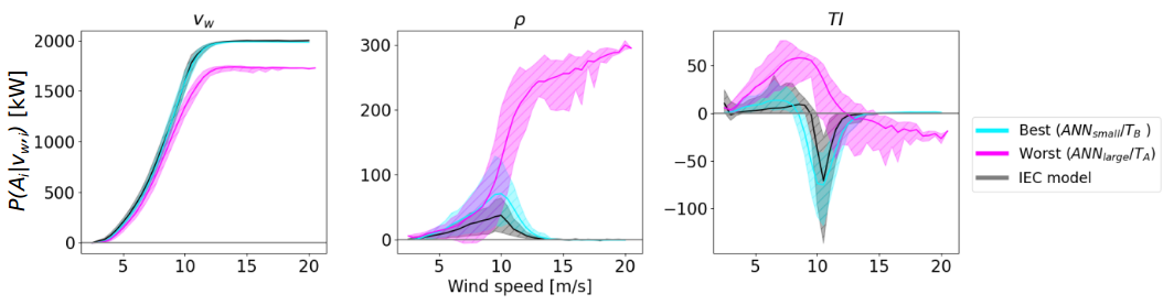
Figure 1: Distributions of attributions (mean as lines, range shaded) conditioned on wind speed ($v_{w}$) by feature (left, center, right). They represent the strategies that agree most (cyan) and least (pink) with the physical benchmark model (grey), and exemplify the wide range of of strategies learned.

As so often, the answer to this question is: it depends. Our results have revealed that ML models can learn a surprisingly wide range of strategies from operational SCADA data, some of which capture physical relationships in an almost textbook-like manner and others that fail to consider them almost entirely. Figure 1 facilitates a comparison between these extreme cases by visualizing strategies for the model with highest ($R^{2}=0.95$ - $ANN_{small}/T_{B}$) and the lowest ($R^{2}=0.47$ - $ANN_{large}/T_{A}$) correlation with the physics informed baseline (also displayed). To understand the reasons, we conduct a systematic analysis of potential impact factors. Figure 2 shows the similarity of learned strategies with the physical baseline for the different models, turbines and input features.

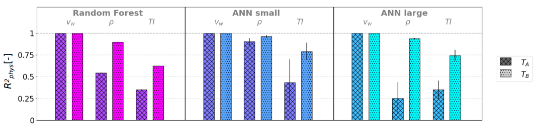
Figure 2: Mean correlation between data-driven and physical IEC model attributions by model (sections/color schemes), input parameter (subsections) and turbine (shade/hash). Error bars to the standard deviation of correlation over 10 training runs with different initializations.

Strategies by input features: intuitive ranking of physical compliance that coincides with the physical importance of the respective input features (influence of $v_{w}$ captured best, $\rho$ mostly reasonable, and $TI$ worst).

Impact of model: $ANN_{large}$ exhibits lower average agreement with IEC model strategies than $RF$ or $ANN_{small}$. The latter learned the most physical strategies across all settings. Also, ANN model initialization can have a profound impact on the learned strategy (see ’error bars’ in Fig. 2).

Impact of turbine: All ML models show higher overall agreement with IEC model strategies on $T_{B}$, large models in particular. The IEC model itself also performs much better on $T_{A}$, indicating that the data set contains less effects beyond the considered physical phenomena.

Implications for model selection: Physically reasonable power curve models are desirable and more robust in out of distribution settings (see App. B). Unfortunately, test-set RMSE is not a good indicator for physical compliance. $ANN_{large}$, for instance, show best performance but largest deviation from physical strategies. Based on our results, we recommend the use of moderately sized ANNs instead (similar to $ANN_{small}$). They have shown clear advantages in terms of strategy at only slightly increased test-set errors compared to $ANN_{large}$ while outperforming $RFs$ in both categories.

3.2 Explaining deviations from an expected turbine output

We demonstrate the importance of appropriate reference points for quantitatively faithful attributions and highlight their potential in the context of performance monitoring.

We utilize a model of type $ANN_{small}$ and include a yaw misalignment feature (details can be found in App. C). This enables experiments in a controlled fashion and a comparison between magnitudes of Shapley attributions ($R_{\Delta_{yaw}}$) and the ground truth ($\Delta P_{yaw}$). We compare attributions for three different reference points (Fig. 3, left): $\widetilde{x}_{min}$ (used for global strategies earlier), $\widetilde{x}_{mean}$ (often the standard choice), and $\widetilde{x}_{informed}$, which incorporates the assumptions implicit to the expected output relative to which we explain (see App. A). The latter clearly outperforms both others in the presented experiment and is, therefore, recommended for this task.

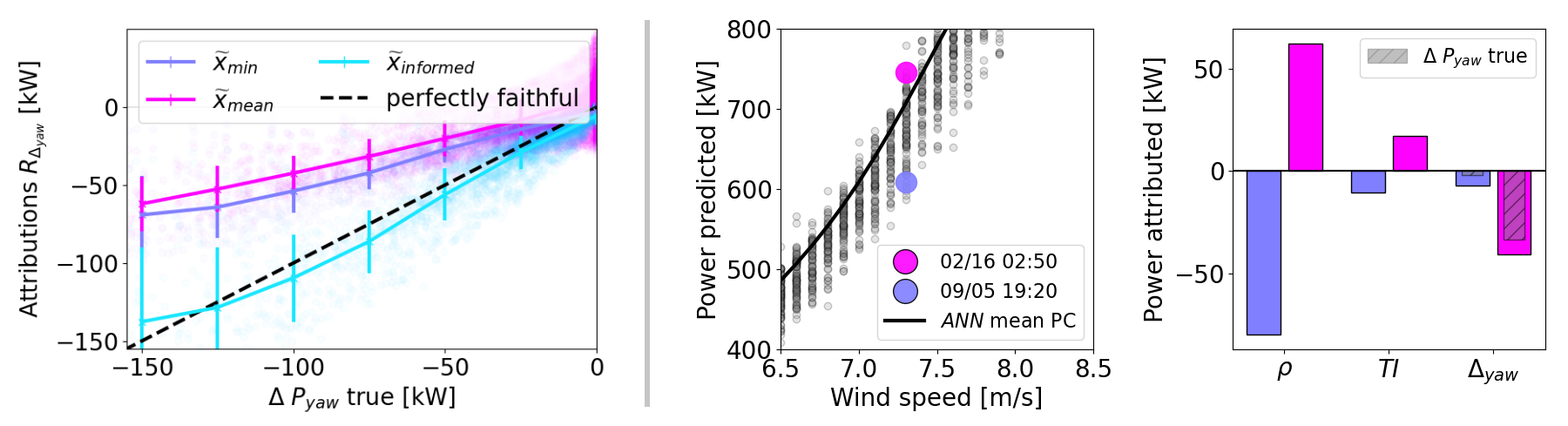
Figure 3: Left: Faithfulness for different reference points ($\widetilde{x}$) - true yaw-induced output reduction vs. respective attributions. Lines display mean and standard deviations over 25 kW bins. Right: two selected data points relative to the learned standard power curve (ANN mean PC), and their respective attributions per input feature.

Once we have ensured physically plausible model strategies and quantitatively faithful attributions, we can utilize the explanations in a performance monitoring context (Fig. 3, right). The first plot shows two selected data points and the learned power curve under mean ambient conditions (no yaw misalignment). Both instances have a low absolute error of $\sim$10 kW. Their position relative to each other and the mean curve suggests that the September instance (violet) is much more likely to be affected by yaw misalignment than the February instance (pink) (higher output at the same wind speed). The respective attributions, however, enable a decomposition and quantification of different entangled effects. In February, significant yaw misalignment was present but compensated by favourable ambient conditions. The September instance’s lower output, on the other hand, can be attributed to less advantageous environmental conditions rather than a technical malfunction. While monitoring yaw misalignment directly would be a trivial solution in this example, this is usually not possible for potential other root causes (blade-pitch-angles or turbine interactions, for example) which can be identified with the approach. Nevertheless, the potential to indicate root causes for underperformance is naturally limited to effects that are correctly captured by the model in the first place. Additionally, the absolute model error should serve as a confidence measure regarding the corresponding attributions (explanations for data points with a low error are more trustworthy).

4 Conclusions

So far, the trend towards ever more complex ML models in data-driven power curve modelling was justified based on superior test-set performance. The results from this contribution suggest, that this might be on the cost of physically reasonable model strategies. These findings remind of the famous Clever-Hans effect in classification Lapuschkin et al. (2019). Whether the deviation from physical intuition can have similarly severe implications here, should be the subject of further research.

Overall, it has to be considered whether a focus on smaller models, that better capture physical phenomena, would be the right way forward. Another benefit of smaller architectures is the reduced carbon footprint when training individual models for each turbine of a large fleet. In any case, we recommend a more prominent role of XAI methods in model selection, since often physically more plausible models were obtained with only minor performance losses. Moreover, we have introduced a practical approach to utilize XAI attributions in a quantitatively faithful manner. This is particularly useful in turbine performance monitoring where the increased transparency can help to identify root causes for underperformance.

With this work, we have laid the foundation for transparent data-driven wind turbine power curve models. We hope that the insights will help practitioners to more effectively utilise their ML models and turbines; along with the related positive implications for the global energy transition.

Appendix A Domain and problem specific reference points

The current practice in the wind domain is to use the mean training input feature vector $\widetilde{x}_{mean}=\bar{X_{tr}}$ (compare e.g. Mathew et al. (2022); Movsessian et al. (2022); Tenfjord & Strand (2020); Pang et al. (2021)). We advocate domain-specific settings for the application to wind turbine power curve models:

Global explanations: For explaining global model strategies, we suggest explaining relative to reference point $\widetilde{x}_{min}=min(X_{tr})$. This generates intuitive attributions relative to wind speed zero (or cut-in, depending on data pre-processing). Plotting their distributions conditioned on the measured wind speed $P(A_{i}|v_{w})$ against the wind speed additionally resembles the way power curves are typically displayed (compare Fig. 1). This facilitates contextualization and interpretation by domain experts.

Local explanations: In the context of wind turbine power curves, the most common question is to explain a deviation from an expected turbine output. This requires $\widetilde{x}$ to reflect the implicit assumptions of that expectation. We suggest the informed reference point ($\widetilde{x}_{informed}$) to be conditioned on $v_{w}$: $x_{ref_{i}}=\mathbb{E}(x_{i}|v_{w})$ for environmental parameters, and set to a healthy parameter baseline for technical parameters (e.g. zero for a yaw misalignment feature).

Appendix B Models and performance

IEC models: For each turbine, we calculate the binned power curve and apply air density, as well as TI corrections following the IEC standard IEC (2017). All required parameterizations for the physics-informed model (binned power curve, average air density and zero TI-reference power curve) are calculated using the training data set. Performance evaluation and explanations are calculated for the test set. More details can be found in IEC 61400-12 IEC (2017).

ML models: hyperparameters which were not specified in the respective publications (training modalities, for example), were selected based on a gird-search with 5-fold cross-validation on the training data set. For evaluation we then report the test set RMSE (mean and standard deviation over 10 training runs with different model initializations). All parameters not further specified were left at the standard settings of the scikit-learn Pedregosa et al. (2011) implementations:

$\bf{RF:}$
RandomForestRegressor(min_samples_split=3, min_samples_leaf=30, n_estimators=100)

$\bf{ANN_{small}}$Schlechtingen et al. (2013):
MLPRegressor(hidden_layer_sizes=(3, 3), activation=’logistic’, learning_rate_init=0.1, learning_rate=’adaptive’, max_iter=10000, tol=10**-6, alpha=0, early_stopping=True, n_iter_no_change=100, verbose=0)

$\bf{ANN_{large}}$ Optis & Perr-Sauer (2019):
MLPRegressor(hidden_layer_sizes=(100, 100, 25), activation=’relu’, learning_rate_init=0.1, learning_rate=’adaptive’, max_iter=10000, tol=10**-6, alpha=0, early_stopping=True, n_iter_no_change=100, verbose=0)

Lastly, we have created an out of distribution scenario to analyse the relation of model strategy and performance. We apply an additional norm filter that removes data points that are further away than 100 MW from the manufacturers standard power curve. We then train the models on the filtered data and evaluate them on the filtered test data (Figure 4, left) and the data during the test period that was removed by the norm-filter (Figure 4, right). The results show, that physically plausible models are more robust in out of distribution scenarios.

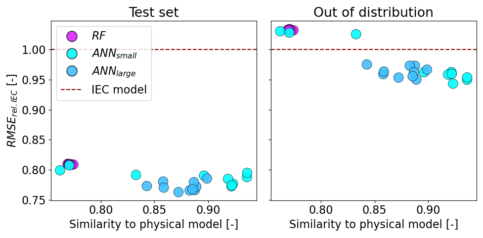
Figure 4: ML model strategy and vs. RMSE for test set (left) and an out of distribution test set (right). Each data point represents a model trained with a different initialization. Results are shown for $T_{B}$.

Appendix C Data augmentation with yaw misalignment

We utilize a model of type $ANN_{small}$ and include the absolute difference between average wind- and nacelle direction as a yaw-misalignment feature ($\Delta_{yaw}$). This allows for experiments in a controlled fashion by augmenting data with artificial yaw-misalignment. This is achieved by adding normally distributed yaw misalignment of up to $\pm 15^{\circ}$ to our data sets, and multiplying the respective targets (turbine output) with a yaw-misalignment factor $c_{ymis,i}=cos^{3}(\Delta_{yaw})$, if $v_{w,i}<v_{rated}$ (approximation derived from the actuator disk model Howland et al. (2020)). After training and evaluation of the model on the augmented data, we can compare magnitude of Shapley attributions to the ground truth:

$$\Delta P_{yaw,i}true=\begin{cases}c_{ymis,i}\cdot P_{T,i},\,&\text{if }v_{w,i}<v_{rated}\\ 0,\,&\text{otherwise}.\end{cases}$$ (1)

References

- Barreto et al. (2021) Guilherme A Barreto, Igor S Brasil, and Luis Gustavo M Souza. Revisiting the modeling of wind turbine power curves using neural networks and fuzzy models: an application-oriented evaluation. Energy Systems, pp. 1–28, 2021.
- Butler et al. (2013) Shane Butler, John Ringwood, and Frank O’Connor. Exploiting scada system data for wind turbine performance monitoring. In 2013 Conference on Control and Fault-Tolerant Systems (SysTol), pp. 389–394, 2013. doi: 10.1109/SysTol.2013.6693951.
- Chatterjee & Dethlefs (2020) Joyjit Chatterjee and Nina Dethlefs. Deep reinforcement learning for maintenance planning of offshore vessel transfer. In Developments in Renewable Energies Offshore, pp. 435–443. CRC Press, 2020.
- Chatterjee & Dethlefs (2021) Joyjit Chatterjee and Nina Dethlefs. Scientometric review of artificial intelligence for operations & maintenance of wind turbines: The past, present and future. Renewable and Sustainable Energy Reviews, 144:111051, 2021. ISSN 1364-0321. doi: https://doi.org/10.1016/j.rser.2021.111051. URL https://www.sciencedirect.com/science/article/pii/S1364032121003403.
- Council (2022) Global Wind Energy Council. Gwec— global wind report 2022. Global Wind Energy Council: Brussels, Belgium, 2022.
- Howland et al. (2020) Michael F Howland, Carlos Moral González, Juan José Pena Martínez, Jesús Bas Quesada, Felipe Palou Larranaga, Neeraj K Yadav, Jasvipul S Chawla, and John O Dabiri. Influence of atmospheric conditions on the power production of utility-scale wind turbines in yaw misalignment. Journal of Renewable and Sustainable Energy, 12(6):063307, 2020.
- IEC (2017) IEC. Wind energy generation systems – part 12-1: Power performance measurements of electricity producing wind turbines. Standard IEC 61400-12-1, International Electrotechnical Commission, Geneva, Switzerland, 2017.
- Janssens et al. (2016) Olivier Janssens, Nymfa Noppe, Christof Devriendt, Rik Van de Walle, and Sofie Van Hoecke. Data-driven multivariate power curve modeling of offshore wind turbines. Engineering Applications of Artificial Intelligence, 55:331–338, 2016.
- Kusiak et al. (2009) Andrew Kusiak, Haiyang Zheng, and Zhe Song. On-line monitoring of power curves. Renewable Energy, 34(6):1487–1493, 2009.
- Lapuschkin et al. (2019) Sebastian Lapuschkin, Stephan Wäldchen, Alexander Binder, Grégoire Montavon, Wojciech Samek, and Klaus-Robert Müller. Unmasking clever hans predictors and assessing what machines really learn. Nature Communications, 10:1096, 2019.
- Letzgus et al. (2022) Simon Letzgus, Patrick Wagner, Jonas Lederer, Wojciech Samek, Klaus-Robert Müller, and Grégoire Montavon. Toward explainable artificial intelligence for regression models: A methodological perspective. IEEE Signal Processing Magazine, 39(4):40–58, 2022. doi: 10.1109/MSP.2022.3153277.
- Lundberg & Lee (2017) Scott M. Lundberg and Su-In Lee. A unified approach to interpreting model predictions. In NIPS, pp. 4765–4774, 2017.
- Mathew et al. (2022) Manuel S Mathew, Surya Teja Kandukuri, and Christian W Omlin. Estimation of wind turbine performance degradation with deep neural networks. In PHM Society European Conference, volume 7, pp. 351–359, 2022.
- Methaprayoon et al. (2007) Kittipong Methaprayoon, Chitra Yingvivatanapong, Wei-Jen Lee, and James R. Liao. An integration of ann wind power estimation into unit commitment considering the forecasting uncertainty. IEEE Transactions on Industry Applications, 43(6):1441–1448, 2007. doi: 10.1109/TIA.2007.908203.
- Montavon et al. (2018) Grégoire Montavon, Wojciech Samek, and Klaus-Robert Müller. Methods for interpreting and understanding deep neural networks. Digital Signal Processing, 73:1–15, 2018.
- Movsessian et al. (2022) Artur Movsessian, David García Cava, and Dmitri Tcherniak. Interpretable machine learning in damage detection using shapley additive explanations. ASCE-ASME Journal of Risk and Uncertainty in Engineering Systems, Part B: Mechanical Engineering, 8(2):021101, 2022.
- Nielson et al. (2020) Jordan Nielson, Kiran Bhaganagar, Rajitha Meka, and Adel Alaeddini. Using atmospheric inputs for artificial neural networks to improve wind turbine power prediction. Energy, 190:116273, 2020.
- Optis & Perr-Sauer (2019) Mike Optis and Jordan Perr-Sauer. The importance of atmospheric turbulence and stability in machine-learning models of wind farm power production. Renewable and Sustainable Energy Reviews, 112:27–41, 2019.
- Pang et al. (2021) Chuanjun Pang, Jianming Yu, and Yan Liu. Correlation analysis of factors affecting wind power based on machine learning and shapley value. IET Energy Systems Integration, 3(3):227–237, 2021. doi: https://doi.org/10.1049/esi2.12022. URL https://ietresearch.onlinelibrary.wiley.com/doi/abs/10.1049/esi2.12022.
- Pedregosa et al. (2011) F. Pedregosa, G. Varoquaux, A. Gramfort, V. Michel, B. Thirion, O. Grisel, M. Blondel, P. Prettenhofer, R. Weiss, V. Dubourg, J. Vanderplas, A. Passos, D. Cournapeau, M. Brucher, M. Perrot, and E. Duchesnay. Scikit-learn: Machine learning in Python. Journal of Machine Learning Research, 12:2825–2830, 2011.
- Pelletier et al. (2016) Francis Pelletier, Christian Masson, and Antoine Tahan. Wind turbine power curve modelling using artificial neural network. Renewable Energy, 89:207–214, 2016.
- Ritchie et al. (2020) Hannah Ritchie, Max Roser, and Pablo Rosado. Co2 and greenhouse gas emissions. Our World in Data, 2020. https://ourworldindata.org/co2-and-other-greenhouse-gas-emissions.
- Samek et al. (2021) Wojciech Samek, Grégoire Montavon, Sebastian Lapuschkin, Christopher J. Anders, and Klaus-Robert Müller. Explaining deep neural networks and beyond: A review of methods and applications. Proceedings of the IEEE, 109(3):247–278, 2021.