The effective complex heavy-quark potential in an anisotropic quark-gluon plasma

Abstract

We introduce a method for reducing anisotropic heavy-quark potentials to isotropic potentials by using an effective screening mass that depends on the quantum numbers $l$ and $m$ of a given state. We demonstrate that, using the resulting 1D effective potential model, one can solve a 1D SchrÃdinger equation and reproduce the full 3D results for the energies and binding energies of low-lying heavy-quarkonium bound states to relatively high accuracy. This includes the splitting of different p-wave polarizations. The resulting 1D effective model provides a way to include momentum anisotropy effects in open quantum system simulations of heavy-quarkonium dynamics in the quark-gluon plasma.

1 Introduction

The survival probability of the heavy quarkonium states, such as $J/\Psi$ and $\Upsilon$ has been widely used as a sensitive probe to study the quark-gluon plasma (QGP) formed in relativistic heavy-ion experiments at RHIC and LHC Matsui:1986dk ; Karsch:1987pv . Due to non-relativistic nature of heavy quarkonium states, one can obtain their in-medium properties, such as masses and decay rates by solving a SchrÃdinger equation with a complex heavy-quark (HQ) potential. The real part of the HQ potential provides the binding energy, whereas the imaginary part provides information about the decay of a quarkonium state via wave function decoherence Laine:2006ns ; Brambilla:2008cx ; Beraudo:2007ky ; Escobedo:2008sy ; Brambilla:2010vq ; Brambilla:2011sg ; Brambilla:2013dpa . One can obtain the HQ potential at short distances by making use of hard-thermal-loop (HTL) resummed perturbation theory in the weak-coupling limit. Recently, several attempts have been made to develop complex-valued potential models to understand the in-medium properties of quarkonia quantitatively Dumitru:2009ni ; Margotta:2011ta ; Strickland:2011mw ; Strickland:2011aa ; Krouppa:2015yoa ; Krouppa:2016jcl ; Krouppa:2017jlg ; Islam:2020gdv ; Islam:2020bnp ; Wen:2022yjx . During the last decade, many prior works have treated the QGP as an anisotropic medium by incorporating momentum-space anisotropies generated by longitudinal expansion into the underlying parton distribution functions. To make a phenomenological study of this effect in heavy-ion collisions, we consider the following spheroidal distribution function ansatz in the local rest frame (LRF) of the QGP Romatschke:2003ms

$$f_{\rm aniso}^{\rm LRF}({\bf k})\equiv f_{\rm iso}\!\left(\frac{1}{\lambda}\sqrt{{\bf k}^{2}+\xi({\bf k}\cdot{\bf n})^{2}}\right)\,.$$ (1)

This form takes into account the rapid longitudinal expansion of the QGP at early times and allows for explicit pressure anisotropies in the LRF Strickland:2014pga ; Berges:2020fwq . Here, $f_{\rm iso}$ is an arbitrary isotropic distribution function, $\lambda$ is a temperature-like scale, which becomes the temperature $T$ of the system in the thermal equilibrium limit. The degree of momentum-space anisotropy ($\xi$) in the range $-1<\xi<\infty$ is given by

$$\xi=\frac{1}{2}\frac{\langle\bf k^{2}_{\perp}\rangle}{\langle k^{2}_{z}\rangle}-1\,,$$ (2)

where $k_{z}\equiv\bf k\cdot n$ and $\bf k_{\perp}\equiv\bf k-\bf n\,(k\cdot n)$ correspond to the particle momenta along and perpendicular to the direction of anisotropy ($\bf{n}$), respectively. Many prior works have studied heavy quarkonium physics by considering the momentum-space anisotropy inside the QGP Strickland:2011aa ; Thakur:2013nia ; Krouppa:2017jlg ; Islam:2020gdv ; Islam:2020bnp ; Dumitru:2009ni ; Romatschke:2003ms ; Strickland:2014pga . Here we focus on how to efficiently take momentum-space anisotropy into account in a one-dimensional effective theory and compare the one- and three-dimensional results for static and dynamical quantities numerically.

In this proceedings contribution, we summarize our previous works where the real part of a 3D anisotropic HQ potential has been reduced to 1D effective potential Dong:2021gnb ; Dong:2022mbo . This work is organized as follow: In sec. 2 we describe the isotropic complex HQ potential model, in sec. 3 we obtain the anisotropic complex HQ potential model, in sec. 4 we obtain our effective complex HQ potential model, in sec. 5 we present our static results, and in sec. 6 we present our dynamic results.

2 Isotropic Potential Model

The Fourier transform of the real time gluon propagator in the static limit gives the complex HQ potential in an isotropic QGP Guo:2018vwy .

$$V(\lambda,r)=-g^{2}C_{F}\int\frac{d^{3}{\bf p}}{(2\pi)^{3}}(e^{i{\bf p}\cdot{\bf r}}-1)D^{00}(p_{0}=0,{\bf p},\lambda)\,.$$ (3)

2.1 Perturbative Contribution

The perturbative contribution to the complex HQ potential can be obtained from HTL resummed perturbation theory. The real and imaginary parts of this perturbative contribution are given by

$${\rm Re}\,V_{\rm pt}(\lambda,r)=-g^{2}C_{F}\int\frac{d^{3}{\bf p}}{(2\pi)^{3}}(e^{i{\bf p}\cdot{\bf r}}-1)\left(\frac{1}{p^{2}+m_{D}^{2}}-\frac{1}{p^{2}}\right)\equiv\alpha m_{D}({\cal I}_{1}({\hat{r}})-1)\,,$$ (4)

$${\rm Im}\,V_{\rm pt}(\lambda,r)=-g^{2}C_{F}\int\frac{d^{3}{\bf p}}{(2\pi)^{3}}(e^{i{\bf p}\cdot{\bf r}}-1)\frac{-\pi\lambda m_{D}^{2}}{p(p^{2}+m_{D}^{2})^{2}}\equiv\alpha\lambda({\cal I}_{2}({\hat{r}})-1)\,,$$ (5)

where the integrals ${\cal I}_{1}({\hat{r}})$ and ${\cal I}_{2}({\hat{r}})$ are

$${\cal I}_{1}({\hat{r}}) = 4\pi\int\frac{d^{3}{\hat{\bf p}}}{(2\pi)^{3}}e^{i{\hat{\bf p}}\cdot{\hat{\bf r}}}\frac{1}{{\hat{p}}^{2}({\hat{p}}^{2}+1)}=\frac{1-e^{-{\hat{r}}}}{{\hat{r}}}\,,$$

$${\cal I}_{2}({\hat{r}}) = 4\pi^{2}\int\frac{d^{3}{\hat{\bf p}}}{(2\pi)^{3}}e^{i{\hat{\bf p}}\cdot{\hat{\bf r}}}\frac{1}{{\hat{p}}({\hat{p}}^{2}+1)^{2}}=\phi_{2}({\hat{r}})\,,$$ (6)

with

$$\phi_{n}({\hat{r}})=2\int_{0}^{\infty}dz\frac{\mathrm{sin}(z{\hat{r}})}{z{\hat{r}}}\frac{z}{(z^{2}+1)^{n}}\,.$$ (7)

Here, ${\hat{\bf p}}\equiv{\bf p}/m_{D}$, ${\hat{\bf r}}\equiv{\bf r}m_{D}$, and the strong coupling constant $\alpha=g^{2}C_{F}/(4\pi)$. We also subtracted a term $1/p^{2}$ in eq. (4) to make the $r$-independent part finite.

2.2 Non-perturbative Contribution

The gluon propagator also contains a non-perturbative string contribution which arises from a dimension two gluon condensate. Its Fourier transform gives us the non-perturbative contributions Guo:2018vwy

$${\rm Re}\,V_{\rm npt}(\lambda,r)=-g^{2}C_{F}m_{G}^{2}\int\frac{d^{3}{\bf p}}{(2\pi)^{3}}(e^{i{\bf p}\cdot{\bf r}}-1)\frac{p^{2}+5m_{D}^{2}}{(p^{2}+m_{D}^{2})^{3}}\equiv-\frac{2\sigma}{m_{D}}({\cal I}_{3}({\hat{r}})-1)\,,$$ (8)

$${\rm Im}\,V_{\rm npt}(\lambda,r)=-g^{2}C_{F}m_{G}^{2}\int\frac{d^{3}{\bf p}}{(2\pi)^{3}}(e^{i{\bf p}\cdot{\bf r}}-1)\frac{4\pi\lambda m_{D}^{2}(p^{2}-2m_{D}^{2})}{p(p^{2}+m_{D}^{2})^{4}}\equiv\frac{4\sigma\lambda}{m_{D}^{2}}({\cal I}_{4}({\hat{r}})-1)\,,$$ (9)

where $\sigma=\alpha m_{G}^{2}/2$ and $m_{G}^{2}$ is a dimensionful constant. The integrals appearing above are

$${\cal I}_{3}({\hat{r}}) = 4\pi\int\frac{d^{3}{\hat{\bf p}}}{(2\pi)^{3}}e^{i{\hat{\bf p}}\cdot{\hat{\bf r}}}\frac{{\hat{p}}^{2}+5}{({\hat{p}}^{2}+1)^{3}}=(1+{\hat{r}}/2)e^{-{\hat{r}}}\,,$$

$${\cal I}_{4}({\hat{r}}) = 8\pi^{2}\int\frac{d^{3}{\hat{\bf p}}}{(2\pi)^{3}}e^{i{\hat{\bf p}}\cdot{\hat{\bf r}}}\frac{2-{\hat{p}}^{2}}{{\hat{p}}({\hat{p}}^{2}+1)^{4}}=-2\phi_{3}({\hat{r}})+6\phi_{4}({\hat{r}})\,.$$ (10)

2.3 Total Isotropic potential

The sum of the perturbative and non-perturbative contributions give us the total complex isotropic HQ potential

$$\mathrm{Re}\,V_{\mathrm{Iso}}(r) = {\rm Re}\,V_{\rm pt}(\lambda,r)+{\rm Re}\,V_{\rm npt}(\lambda,r)$$ (11)

$$= \alpha m_{D}\left(\frac{1-e^{-rm_{D}}}{rm_{D}}\right)-\alpha m_{D}-\frac{\sigma}{m_{D}}\left(2+rm_{D}\right)e^{-rm_{D}}+\frac{2\sigma}{m_{D}}-\frac{\alpha}{r}\,,$$

$$\mathrm{Im}\,V_{\mathrm{Iso}}(r) = {\rm Im}\,V_{\rm pt}(\lambda,r)+{\rm Im}\,V_{\rm npt}(\lambda,r)$$ (12)

$$= \alpha\lambda\phi_{2}\left(rm_{D}\right)-\alpha\lambda-\frac{8\sigma\lambda}{m_{D}^{2}}\phi_{3}(rm_{D})+\frac{24\sigma\lambda}{m_{D}^{2}}\phi_{4}(rm_{D})-\frac{4\sigma\lambda}{m_{D}^{2}}\,.$$

We include a relativistic correction, $-0.8\sigma/(m_{b/c}^{2}r)$, in the potential model while solving the Schrödinger equation for charmonia and bottomonia Dumitru:2009ni , where the masses of the charm and bottom quarks are taken to be $m_{c}=1.3\,{\rm GeV}$ and $m_{b}=4.7\,{\rm GeV}$, respectively.

3 3D Anisotropic Potential Model

The real and imaginary part of the 3D anisotropic potential model as derived in our previous work Dong:2022mbo are

$$\mathrm{Re}\,V_{\mathrm{Aniso}}(r,\theta,\xi)=\alpha m_{D}^{A}\left(\frac{1-e^{-rm_{D}^{R}}}{rm_{D}^{R}}\right)-\alpha m_{D}^{A}-\frac{\sigma}{m_{D}^{A}}\left(2+rm_{D}^{R}\right)e^{-rm_{D}^{R}}+\frac{2\sigma}{m_{D}^{A}}-\frac{\alpha}{r}\,,$$ (13)

$$\mathrm{Im}\,V_{\mathrm{Aniso}}(r,\theta,\xi)=\alpha\lambda^{A}\phi_{2}\left(rm_{D}^{I}\right)-\alpha\lambda^{A}-\frac{8\sigma\lambda^{A}}{\left(m_{D}^{A}\right)^{2}}\phi_{3}\left(rm_{D}^{I}\right)+\frac{24\sigma\lambda^{A}}{\left(m_{D}^{A}\right)^{2}}\phi_{4}\left(rm_{D}^{I}\right)-\frac{4\sigma\lambda^{A}}{\left(m_{D}^{A}\right)^{2}}\,,$$ (14)

where,

$$m_{D}^{A}=m_{D}\left(1-\frac{\xi}{6}\right)\,,\quad\lambda^{A}=\lambda\left(1-\frac{\xi}{6}\right),$$ (15)

and

$$m^{R}_{D}=m_{D}\bigg{[}1+\xi\left(0.108\cos 2\theta-0.131\right)\bigg{]}\,,\quad m^{I}_{D}=m_{D}\bigg{[}1+\xi\left(0.026\cos 2\theta-0.158\right)\bigg{]}.$$ (16)

Eq(15) assures a correct asymptotic behavior of the potential. Eq. (16) was obtained by matching effective and exact result at ${\hat{r}}=1$ as described in  Dong:2022mbo .

4 1D Effective Potential Model

Due to the angular dependence in the 3D anisotropic potential model, solving a 3D Schrödinger equation to find various in-medium properties of the quarkonium states is rather time consuming and much more complicated. One possible solution to this problem is to introduce an angle-averaged effective screening mass ${\cal{M}}_{lm}(\lambda,\xi)$  Dong:2021gnb

$${\cal{M}}^{R,I}_{lm}(\lambda,\xi) = \langle{\rm{Y}}_{lm}(\theta,\phi)|m^{R,I}_{D}(\lambda,\xi,\theta)|{\rm{Y}}_{lm}(\theta,\phi)\rangle\,,$$ (17)

$$= \int_{-1}^{1}d\cos\theta\int_{0}^{2\pi}d\phi{\rm{Y}}_{lm}(\theta,\phi)m^{R,I}_{D}(\lambda,\xi,\theta){\rm{Y}}^{*}_{lm}(\theta,\phi)\,,$$

and where ${\rm{Y}}_{lm}(\theta,\phi)$ refers to the spherical harmonics with azimuthal quantum number $l$ and magnetic quantum number $m$. The main advantage of using an angle-averaged effective screening mass ${\cal{M}}_{lm}(\lambda,\xi)$ is to utilize the spherical symmetry in the potential model which significantly simplifies the numerics.

The real and imaginary part of the 1D effective potential model as derived in our previuos work Dong:2022mbo are

$$\mathrm{Re}\,V_{\mathrm{Eff}}(r,\xi)=\alpha m_{D}^{A}\left(\frac{1-e^{-r{\cal{M}}_{lm}^{R}}}{r{\cal{M}}_{lm}^{R}}\right)-\alpha m_{D}^{A}-\frac{\sigma}{m_{D}^{A}}\left(2+r{\cal{M}}_{lm}^{R}\right)e^{-r{\cal{M}}_{lm}^{R}}+\frac{2\sigma}{m_{D}^{A}}-\frac{\alpha}{r}\,,$$ (18)

$$\mathrm{Im}\,V_{\mathrm{Eff}}(r,\xi)=\alpha\lambda^{A}\phi_{2}\left(r{\cal{M}}_{lm}^{I}\right)-\alpha\lambda^{A}-\frac{8\sigma\lambda^{A}}{\left(m_{D}^{A}\right)^{2}}\phi_{3}\left(r{\cal{M}}_{lm}^{I}\right)+\frac{24\sigma\lambda^{A}}{\left(m_{D}^{A}\right)^{2}}\phi_{4}\left(r{\cal{M}}_{lm}^{I}\right)-\frac{4\sigma\lambda^{A}}{\left(m_{D}^{A}\right)^{2}}\,,$$ (19)

where,

$$K_{lm}=\frac{2l(l+1)-2m^{2}-1}{4l(l+1)-3}\,$$ (20)

and

$${\cal{M}}_{lm}^{R}=m_{D}\bigg{[}1+\xi\left(0.216K_{lm}-0.239\right)\bigg{]}\leavevmode\nobreak\ ,\quad{\cal{M}}_{lm}^{I}=m_{D}\bigg{[}1+\xi\left(0.052K_{lm}-0.184\right)\bigg{]}.$$ (21)

The $l$ and $m$ values of various quarkonium states are given in Table 1.

Table 1: $l$ and $m$ values of various quarkonium states.

5 Static Results

For the static solutions, we used a previously developed 3D eigensolver called quantumFDTD Strickland:2009ft ; Delgado:2020ozh . Using this code, we compared results obtained with the 1D effective potential and the full 3D anisotropic potential. In Table 2, we list the exact results of the eigenenergies (${\rm Re}\,E$), decay widths (${\rm Im}\,E$) and the binding energies ($E_{\rm bind}$) with the anisotropy parameter $\xi=1$ for $\Upsilon(1S)$ and $J/\Psi$.

In the numerical evaluations, we took $\alpha=0.272$ and $\sigma=0.215\,{\rm GeV}^{2}$. For the $\Upsilon(1S)$ state, we used a lattice size of $N^{3}=512^{3}$ with a lattice spacing of $a=0.020\,{\rm GeV}^{-1}\approx 0.004\,{\rm fm}$ giving a lattice size of $L=Na\approx 2.05\,{\rm fm}$. For the $J/\psi$, we used a lattice size of $N^{3}=256^{3}$ with a lattice spacing of $a=0.085\,{\rm GeV}^{-1}\approx 0.017\,{\rm fm}$ giving a lattice size of $L=Na\approx 4.35\,{\rm fm}$.

$\Upsilon(1S)$	${\rm Re}E$	$\delta{\rm Re}E$	$E_{\rm bind}$	${\rm Im}E$	$\delta{\rm Im}E$
$T_{o}$	$182.869$	$0.611$	$-662.669$	$11.838$	$0.027$
$1.1T_{o}$	$174.957$	$0.593$	$-570.612$	$14.830$	$0.031$
$1.2T_{o}$	$166.556$	$0.573$	$-493.689$	$18.190$	$0.034$
$1.4T_{o}$	$148.439$	$0.531$	$-372.540$	$26.004$	$0.039$

$J/\Psi$	${\rm Re}E$	$\delta{\rm Re}E$	$E_{\rm bind}$	${\rm Im}E$	$\delta{\rm Im}E$
$T_{o}$	$439.336$	$1.230$	$-406.202$	$41.980$	$0.107$
$1.1T_{o}$	$422.207$	$1.163$	$-323.362$	$51.467$	$0.105$
$1.2T_{o}$	$404.597$	$1.095$	$-255.648$	$61.698$	$0.098$
$1.3T_{o}$	$386.604$	$1.028$	$-199.583$	$72.564$	$0.086$
$1.4T_{o}$	$368.301$	$0.963$	$-152.678$	$83.958$	$0.070$

Table 2: The exact 3D results of the complex eigenenergies ($E$) and binding energies ($E_{\rm bind}$) for different quarkonium states at various temperatures with $\xi=1$. $\delta E$ are the differences in results obtained using 1D effective and 3D anisotropic potentials. Here $T_{o}$ is $192\,{\rm{MeV}}$ and all results are in MeV Dong:2022mbo .

6 Dynamical Results

In order to solve the 3D Schrödinger equation in real time, we used a split-step pseudospectral method Taha:1984jz with temporal step size $\Delta t=0.001$ fm/c. Once again we compare results obtained with the full 3D anisotropic potential to those obtained with the 1D effective potential. We evolve the wave function from $\tau=0$ fm/c to $\tau=0.25$ fm/c in the vacuum ($T=0$). Starting at $\tau=\tau_{0}=0.25$ fm/c, we consider a fixed anisotropy parameter $\xi=1$ and boost-invariant Bjorken evolution for the hard scale

$$\lambda(\tau)=\lambda_{0}\left(\frac{\tau_{0}}{\tau}\right)^{1/3}\,.$$ (22)

Here we take the initial hard scale to be $\lambda_{0}=$ 630 MeV. Further details of the numerical method can be found in  Dong:2022mbo .

6.1 Bottomonium

For bottomonium states we take the box size to be $L=$ 2.56 fm, $m_{b}=4.7$ GeV, and use $N=128$ lattice points in each direction. The top row of fig. 1 shows the time evolution of overlaps of the $\Upsilon(1S)$, $\Upsilon(2S)$, and $\Upsilon(3S)$ using a pure $\Upsilon(1S)$ eigenstate as the initial condition. Whereas the bottom row shows the time evolution of the bottomonium p-wave overlaps resulting from initialization with different p-wave polarizations. Results with pure $\Upsilon(2S)$ and $\Upsilon(3S)$ eigenstates and a Gaussian as the initial condition can be found in Ref. Dong:2022mbo .

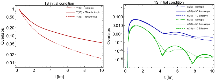
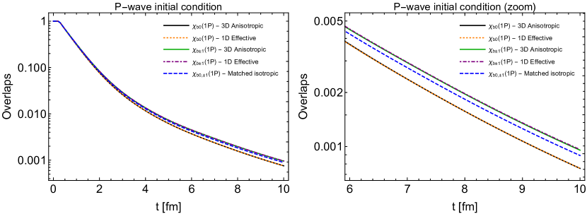
Figure 1: The top row shows the overlaps of $\Upsilon(1S)$, $\Upsilon(2S)$, and $\Upsilon(3S)$ resulting from real-time solution of the Schrödinger equation. Here we initialized the wave function as pure $\Upsilon(1S)$ eigenstate. The bottom row shows the time evolution of the bottomonium p-wave overlaps resulting from initialization with different p-wave polarizations Dong:2022mbo .

6.2 Charmonium

For charmonium states we take $L=$ 5.12 fm, $m_{c}=1.3$ GeV, and use $N=128$ lattice points in each direction. The top row of the fig. 2 shows the time evolution of overlaps of the $J/\psi$, $\psi(2S)$, and $\psi(3S)$ by using pure $J/\psi$ eigenstate as the initial condition. Whereas the bottom row shows the time evolution of the charmonium p-wave overlaps resulting from initialization with different p-wave polarizations. The results with pure $\psi(2S)$ and $\psi(3S)$ eigenstate and Gaussian as the initial condition can be found in Ref. Dong:2022mbo .

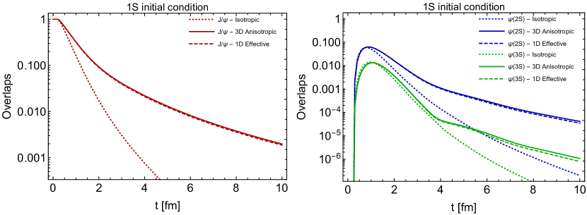
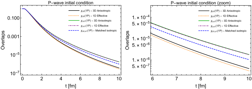
Figure 2: The top row shows the overlaps of $J/\psi$, $\psi(2S)$, and $\psi(3S)$ resulting from real-time solution of the Schrödinger equation. Here we initialized the wave function as pure $J/\psi$ eigenstate. The bottom row shows the time evolution of the charmonium p-wave overlaps resulting from initialization with different p-wave polarizations Dong:2022mbo .

7 Conclusions

We have reduced anisotropic heavy-quark potentials to isotropic ones by introducing an effective screening mass that depends on the quantum numbers $l$ and $m$ of a given state. We demonstrated that, using the resulting 1D effective potential model, one can reproduce the full 3D results for the energies and binding energies of low-lying heavy-quarkonium bound states to relatively high accuracy. This finding is important because it can be used to incorporate anisotropy effects into one-dimensional real-time Schrödinger equations which underpin phenomenological calculations of bottomonium suppression in open quantum systems approaches.

References

- (1) T. Matsui, H. Satz, Phys. Lett. B 178, 416 (1986)
- (2) F. Karsch, M.T. Mehr, H. Satz, Z. Phys. C 37, 617 (1988)
- (3) M. Laine, O. Philipsen, P. Romatschke, M. Tassler, JHEP 03, 054 (2007), hep-ph/0611300
- (4) N. Brambilla, J. Ghiglieri, A. Vairo, P. Petreczky, Phys. Rev. D 78, 014017 (2008), 0804.0993
- (5) A. Beraudo, J.P. Blaizot, C. Ratti, Nucl. Phys. A 806, 312 (2008), 0712.4394
- (6) M.A. Escobedo, J. Soto, Phys. Rev. A 78, 032520 (2008), 0804.0691
- (7) N. Brambilla, M.A. Escobedo, J. Ghiglieri, J. Soto, A. Vairo, JHEP 09, 038 (2010), 1007.4156
- (8) N. Brambilla, M.A. Escobedo, J. Ghiglieri, A. Vairo, JHEP 12, 116 (2011), 1109.5826
- (9) N. Brambilla, M.A. Escobedo, J. Ghiglieri, A. Vairo, JHEP 05, 130 (2013), 1303.6097
- (10) A. Dumitru, Y. Guo, A. Mocsy, M. Strickland, Phys. Rev. D 79, 054019 (2009), 0901.1998
- (11) M. Margotta, K. McCarty, C. McGahan, M. Strickland, D. Yager-Elorriaga, Phys. Rev. D 83, 105019 (2011), [Erratum: Phys.Rev.D 84, 069902 (2011)], 1101.4651
- (12) M. Strickland, Phys. Rev. Lett. 107, 132301 (2011), 1106.2571
- (13) M. Strickland, D. Bazow, Nucl. Phys. A 879, 25 (2012), 1112.2761
- (14) B. Krouppa, R. Ryblewski, M. Strickland, Phys. Rev. C 92, 061901 (2015), 1507.03951
- (15) B. Krouppa, M. Strickland, Universe 2, 16 (2016), 1605.03561
- (16) B. Krouppa, A. Rothkopf, M. Strickland, Phys. Rev. D 97, 016017 (2018), 1710.02319
- (17) A. Islam, M. Strickland, Phys. Lett. B 811, 135949 (2020), 2007.10211
- (18) A. Islam, M. Strickland, JHEP 21, 235 (2020), 2010.05457
- (19) L. Wen, B. Chen (2022), 2208.10050
- (20) P. Romatschke, M. Strickland, Phys. Rev. D 68, 036004 (2003), hep-ph/0304092
- (21) M. Strickland, Acta Phys. Polon. B 45, 2355 (2014), 1410.5786
- (22) J. Berges, M.P. Heller, A. Mazeliauskas, R. Venugopalan, Rev. Mod. Phys. 93, 035003 (2021), 2005.12299
- (23) L. Thakur, U. Kakade, B.K. Patra, Phys. Rev. D 89, 094020 (2014), 1401.0172
- (24) L. Dong, Y. Guo, A. Islam, M. Strickland, Phys. Rev. D 104, 096017 (2021), 2109.01284
- (25) L. Dong, Y. Guo, A. Islam, A. Rothkopf, M. Strickland, JHEP 09, 200 (2022), 2205.10349
- (26) Y. Guo, L. Dong, J. Pan, M.R. Moldes, Phys. Rev. D 100, 036011 (2019), 1806.04376
- (27) M. Strickland, D. Yager-Elorriaga, J. Comput. Phys. 229, 6015 (2010), 0904.0939
- (28) R.L. Delgado, S. Steinbeißer, M. Strickland, J.H. Weber, Comput. Phys. Commun. 272, 108250 (2022), 2006.16935
- (29) T.R. Taha, M.J. Ablowitz, J. Comput. Phys. 55, 203 (1984)