Bisparse Blind Deconvolution through Hierarchical Sparse Recovery

Abstract

The bi-sparse blind deconvolution problem is studied – that is, from the knowledge of $h*(Qb)$, where $Q$ is some linear operator, recovering $h$ and $b$, which are both assumed to be sparse. The approach rests upon lifting the problem to a linear one, and then applying the hierarchical sparsity framework. In particular, the efficient HiHTP algorithm is proposed for performing the recovery. Then, under a random model on the matrix $Q$, it is theoretically shown that an $s$-sparse $h\in\mathbb{K}^{\mu}$ and $\sigma$-sparse $b\in\mathbb{K}^{n}$ with high probability can be recovered when $\mu\gtrsim s^{2}\log(\mu)+s^{2}\sigma\log(n)$.

I Introduction

We begin by motivating and illustrating the bi-sparse deconvolution problem within a simple communication scenario. Consider two persons, Alice and Bob, communicating with each other. Bob would like to send a message $b\in\mathbb{K}^{n}$, where $\mathbb{K}$ denotes one of the fields $\mathbb{R}$ or $\mathbb{C}$, to Alice. To do so, he first linearly encodes his message in a signal $Qb\in\mathbb{K}^{\mu}$, and then sends it over a wireless channel to Alice. Due to scattering in the environment, Alice will not receive $Qb$, but rather a superposition of several time and phase-shifted versions of the signal $Qb$. Put differently, she will observe the convolution

$$y=h*(Qb)$$

of $Qb$ with a filter $h\in\mathbb{K}^{\mu}$ modelling the impulse response of the environment. A schematic sketch is provided in Figure 1. The filter $h$ will be highly dependent on largely unknown features of the environment. In traditional communication protocols, Alice determine the filter $h$ prior to the actual communication by receiving an pre-determined pilot signals from Bob through the channel. Interesting alternative approaches are presented by blind communication protocols that omit the separate channel estimation stage. In order to retrieve the message $b$, Alice here needs to solve a blind deconvolution problem, i.e. determine $b$ given $y$ and $Q$ but without knowledge of $h$. Since the scattered signal typically only reaches the receiver antenna along a few, distinct paths, it is reasonable to assume that the filter $h$ is sparse [1]. We can furthermore render the message $b$ sparse by system design. Under these assumption we arrive at a bi-sparse blind deconvolution problem. In the following we will denote the sparsity of $h$ and $b$ by $s$ and $\sigma$, respectively.

Figure 1: Our communication model.

I-A Related work.

The approaches to solving the sparse blind deconvolution problem can broadly be divided into two overarching categories:

• Solve the problem via minimizing a function of the form

  $$L:\mathbb{K}^{\mu}\times\mathbb{K}^{n}\to\mathbb{R},\quad(h,b)\mapsto L(h,b)=\mathcal{L}(y,h*(Qb),h,b),$$

  defined in terms of a suitable loss function $\mathcal{L}$. Let us call such methods direct.

• Using the universal property of tensor spaces, identify the bilinear map $\gamma(h,b)=h*Qb$ on $\mathbb{K}^{\mu}\times\mathbb{K}^{n}$ with a linear map $\mathcal{C}$ on $\mathbb{K}^{\mu}\otimes\mathbb{K}^{n}$, and then minimize

  $$K:\mathbb{K}^{\mu}\otimes\mathbb{K}^{n}\to\mathbb{R},\quad w\mapsto K(w)={\mathcal{L}}(y,\mathcal{C}(w),w).$$

  Effectively, we go over from recovering the pair $(h,b)$ to recovering the tensor $h\otimes b$. This procedure is generally referred to as lifting, and we will here refer to them as lifted methods.

Let us give a brief overview of some results from the literature about methods from both families. Throughout the discussion, it is instructive to consider that the optimal sample complexity (i.e. the number of needed observations to enable injectivity) are given by $(\mu+n)$ in the non-sparse setting and $(s+\sigma)$ in the sparse setting [2, 3].

Direct approaches

As for the direct approaches, the alternating minimization technique is probably the most prominent. It was introduced in [4] as a means for solving the so called phase retrieval problem. It was later adapted to blind deconvolution in [5, 6]. The alternating minimization techniques generally refers to alternating between solving the two problems,

$$\operatorname*{minimize}_{h\text{ (sparse) }}\ L(h,b^{\prime})\quad\text{and}\quad\operatorname*{minimize}_{b\text{ (sparse) }}\ L(h^{\prime},b).$$

Since the convolution is linear in each argument, each subproblem is effectively a classical compressed sensing problem, and can be solved using a number of technique, e.g. iterative hard thresholding [7] or CoSAMP [8].

As for success of alternating minimization, the authors of [5, 6] give a recovery guarantee in a special setting: First, they use a a generic subspace model - that is, they assume that also $h$ has a representation $h=Bg$ for some $s$-sparse vector $g$, rather than being sparse itself, and $B$ is assumed to be matrix with Gaussian entries. The measurement matrix $Q$ is also assumed to be Gaussian. Crucially, they make the assumption that $h$ and $x=Qb$ are spectrally flat, meaning that their Fourier transforms have approximately constant amplitude. The spectral flatness assumption is not only a regularity assumption on the signals, but it is actively used via a projection step in their algorithm. This projection step is hard to perform exactly, and the authors need to resort to heuristics to resolve that step. However, accepting this caveat, the authors prove convergence already when only observing $(s+\sigma)\log(\mu)^{5}$ of the entries in $h*x$, which is up to log-terms sample optimal.

In [9], Li, Ling, Strohmer and Wei proposed a different non-convex approach for the related problem where $h$ and $b$ are in a known subspaces. Concretely, they assume that $h$ is the Fourier transform of a vector $g\in\mathbb{C}^{\mu}$ supported on its first $s$ entries (rather than being $s$-sparse), and $b=Bc$ for some $c\in\mathbb{C}^{\sigma}$ and $B$ a Gaussian. Needless to say, this variation of the problem amounts to a significant simplification. For a non-convex, smooth, loss function including regularization terms, together with a careful initialization, they prove convergence. They also assume a spectral flatness condition. This assumption is again built into the method, now implicitly in that it governs the size of a constant in the loss function. They prove global convergence already when $\mu\gtrsim\max(s,\sigma)\log(\mu)^{2}$. Note that in our setting, where the supports of the vectors are unknown, this condition would read $\mu\gtrsim\max(\mu,n)\log(\mu)^{2}$, which would be vacuous.

Lifted approaches

As for lifted approach, it is crucial to understand that the lifted ground truth signal $h_{0}\otimes b_{0}$ or equivalently its matrix form $h_{0}b_{0}^{*}$, where $b_{0}^{*}$ denotes the Hermitian transpose of $b_{0}$, simultaneously enjoys two structures: it has rank one and is sparse (in a structured manner). Each of these structures can individually be exploited using convex regularizers – if we take the low-rank property as the crucial one, the nuclear norm is the canonical regularizer [10, 11, 12], whereas if the sparsity is taken as the crucial property, the $\ell_{1}$-norm [13] or its relative, the $\ell_{1,2}$-norm [14] should be used. While the convex approaches are stable, mathematically pleasing and can be globally solved by off-the-shelf algorithms, they are computationally intensive and, thus, often impractical. Furthermore, recovery guarantees are only known for generic subspace models. Under similar assumption of known supports as above, the nuclear norm approach recovers the ground truth when $\mu\gtrsim\max(s,\sigma)\log(\mu)^{2}$ [11, 12, 15]. However, not assuming know supports, that guarantee degenerates to $\mu\gtrsim\max(\mu,n)\log(\mu)^{2}$. The sparse models ($\ell_{1}$ and $\ell_{1,2}$) recover the ground truth with high probability when $\mu\gtrsim s\sigma\log(sn)\log(\mu)^{2}$ under the assumption that the support of $h$ is known [13, 14]. If the the support of $h$ is not known, the guarantee again degenerates to $\mu\gtrsim\mu\sigma\log(n)\log(\mu)^{2}$.

There also is a natural non-convex-way to solve the lifted problem: a gradient descent projected onto the set of (bi)-sparse and low-rank matrices. As is thorougly discussed in [16], there is however no practical algorithm available to compute this projection. The bi-sparse unit-rank projection is known as the sparsePCA problem, that has been shown to be worst-case NP-hard, as well as under approximation and on average [17, 18, 19]. A canonical way to circumvent this obstacle is to alternate between projections onto the two sets. This approach is for instance investigated in [20]. There, a local convergence guarantee is presented under optimal sample complexity using the considerably simpler a measurement model with a Gaussian linear map without the structure of the convolution. Similar results are given in [21] for an alternating minimization approach, this guarantee is however only sample optimal under an additional assumption on the signal.

In this context, [22] should also be mentioned - these authors obtain global convergence in just two alternations steps, however by assuming a nested measurement structure tailor-made for a jointly low-rank and sparse setting, which is often not given.

The findings of this literature review can be summarized as follows.

• Direct methods. These operate at optimal sample complexity, however only under complicated additional assumptions. Furthermore, they typically rest upon a good initialisation.

• Lifted methods. There are convex and non-convex approaches to solve the lifted problems. The convex ones converge globally and are simple to implement, but are computationally heavy and cannot recover the signals at optimal sample complexity. Furthermore, their convergence can only be guaranteed when either the filter or the signal a-priori has known support.

  The non-convex ones are fast and converge quickly, but only work sample-optimally when computationally intractable projection routines are assumed. When heuristics and approximations of the projection steps are applied instead, only local convergence results are known for practical measurement models.

I-B Contribution

In this work, we propose a new, non-convex, approach to the problem, namely to solve the lifted problem as an hierarchically sparse recovery problem. Notice that if both $h$ and $b$ are sparse, the lifted-ground truth signal in its matrix form $w=h_{0}b^{*}$ only has $s$ non-zero rows, and each row is a $\sigma$-sparse vector itself. This is an example of an $(s,\sigma)$-hierarchically sparse signal [23, 24, 25, 26, 27]. The signal $w$ has in fact even more structure such as a joint row-support due to the low-rank. At the core of our approach, however, is to only explicitly exploit the hierarchical sparse structure. In [28], a subset of the authors showed that such signals can be effectively reconstructed from linear measurements using a hard-thresholding algorithm. This type of algorithmic modifications can be regarded as a special case of model based compressed sensing [29]. The algorithm in each step estimates the the sparse support from a gradient step to minimize the residual via projection onto the set of hierarchically sparse vectors, and subsequently solves the least squares problem restricted to the support estimate. The resulting algorithm is called HiHTP, Hierarchical Hard Thresholding Pursuit – the hierarchical variant of the HTP of Ref. [7]. A formal definition of the algorithm is given later in the paper (Algorithm 1).

Crucially, the projection step of HiHTP is computationally efficient. The algorithm can further be proven to recover the ground truth in a stable and robust fashion under a suitable restricted isometry condition (RIP). We refer to Ref. [27] for a more detailed overview of the framework.

Using HiHTP for bisparse blind deconvolution was proposed and numerically demonstrated to work by a subset of the authors in [30]. In the present paper, we provide a theoretical recovery guarantee for its success. The main result can be qualitatively stated as follows:

Main Result.

Suppose $y=h\ast(Qb)\in\mathbb{K}^{\mu}$ with $b\in\mathbb{K}^{n}$ $\sigma$-sparse, $h\in\mathbb{K}^{\mu}$ $s$-sparse and $Q$ Gaussian. Suppose

$$\mu\gtrsim s^{2}\log(\mu)+s^{2}\sigma\log(n),$$

the HiRIP-algorithm will with high probability recovery the ground truth signal $h\otimes b$ from $y$ and $Q$.

Disregarding logarithmic terms, our bound is of the order $s^{2}\sigma$ in the sparsity parameters $s$ and $\sigma$. This is of course not even close to the sample optimal number $(s+\sigma)$ of measurements. At the same time it seems close-to-optimal compared to what one can achieve with a hierarchically sparse relaxation of the original problem structure. Note that the HiHTP-algorithm would work equally well when the measurements originated from a hierarchically sparse signal $(w_{1},\dots,w_{n})$ where the blocks are not equal. Counting the degrees of freedom of the hierarchical sparse vector, thus, suggest an optimal sample complexity of $s\cdot\sigma$. The result here has an additional factor of $s$, that we believe to be an artefact of the proof. In the final part of the paper, we support this claim with a small numerical study, which suggests that the number of measurement the algorithm needs only scales linearly with $s$.

Compared to the existing guarantees for direct approaches, we however do not require a spectral-flatness condition, a generic dictionary for $h$ and a heuristic projection step or known subspaces. Compared to the existing lifted approaches, our guarantee has an improved sampling complexity in the bi-sparse setting with unknown supports. Thus, although the sample complexity of our proof is not optimal, it solves either a ‘harder’ problem or works under more general conditions than the methods available in the literature.

A feature of the hierarchical sparse approach to sparse deconvolution problems is that it readily generalizes to more complicated settings, e.g. arising in a multi-user communication. In addition to the above result, we also discuss how to solve a combined deconvolution and demixing problem using the hierarchically sparse framework: Given $M$ measurements of the form

$$y_{q}=\sum_{p\in[N]}d_{qp}h^{p}*(Q_{p}b^{p}),$$

where $d_{qp}\in\mathbb{K},\ q\in[M],p\in\mathbb{K}$ are ‘mixing scalars’, how do we recover the collection of $N$ filter-signal pairs $(h^{p},b^{p}),p\in[N]$. This problem instance, e.g., appears when users are separated both through their spatial angles and their multipath delay as in [31]. Under the assumption that only $S$ filters/messages are non-zero, we can interpret this again as an hierarchical sparse recovery problem (albeit now in three levels of hierarchy). Using recent results from [32], we show that if each matrix $Q_{p}$ is constructed as above, HiHTP can recover all signals and all filters from $M\gtrsim S\log(N)$ mixtures.

I-C Outline of the paper

In Section II, we give a formal introduction to our approach and our assumptions, and also formally state the main result, Theorem II.1. We also briefly discuss the multi-user setup there. Section III is in its entirety devoted to proving the main result. In Section IV, we briefly numerically investigate the achievable scaling.

Notation

Most of the notation will be either be standard or be introduced when used for the first time. Let us however now already agree that for a vector $v\in\mathbb{F}^{n}$, we will interchangedly use $[v]_{i}$, $v(i)$ and $v_{i}$ to denote its $i$:th entry. Also, we will use $\|\,\cdot\,\|$ to denote the euclidean norm for both vectors and tensors, $\|\,\cdot\,\|_{F}$ for the Frobenius norm for matrices, and $\|\,\cdot\,\|_{2\to 2}$ for the induced $\ell_{2}\to\ell_{2}$-operator norm for matrices. Finally, we denote by $\gtrsim$ ordering up-to a constant factor that does not dependent on the stated variables.

II Bisparse blind deconvolution with HiHTP

Let us first agree on some notation. As outlined above, we are interested in the blind deconvolution program, i.e. recovering $h\in\mathbb{K}^{\mu}$ and $x\in\mathbb{K}^{\mu}$ from the convolution $h*x$. We thereby understand the convolution as circular, i.e.

$$[h\ast x]_{\ell}=\sum_{k\in[\mu]}h_{\ell-k}x_{k}\,,$$ (1)

Here, $[\mu]$ is the set of reminder classes modulo $\mu$, i.e. the set of non-negative integers from $0$ to $(\mu-1)$ equipped with the addition modulo $\mu$. In the following also all indices are understood using this cyclic identification.

Let us state the formal assumptions on the filter and message vectors $h$ and $x$.

Assumption 1.

We assume that

• The filter $h\in\mathbb{K}^{\mu}$ is $s$-sparse.

• The signal $x\in\mathbb{K}^{\mu}$ has a $\sigma$-sparse representation in a dictionary $Q\in\mathbb{K}^{\mu,n}$. That is, there exists a $\sigma$-sparse vector $b\in\mathbb{K}^{n}$ with $x=Qb$.

Lifting

The map $(h,b)\mapsto h*(Qb)$ is bilinear, and can therefore be lifted to a linear map $\mathcal{C}:\mathbb{K}^{n}\otimes\mathbb{K}^{\mu}\cong(\mathbb{K}^{n})^{\mu}\to\mathbb{K}^{\mu}$ by linearly extending

$${h\otimes b\mapsto}\mathcal{C}(h{\otimes}b)=h*(Qb)\,.$$ (2)

This means that we can interpret the blind deconvolution problem as a linear reconstruction problem for the lifted vector $h\otimes b\in\mathbb{R}^{\mu}\otimes\mathbb{R}^{n}$. The idea of this paper is to utilize that the sparsity assumptions on $h$ and $b$ implies that the lifted vector has a particular structure: Among others, it is hierarchically sparse [28]. Let $\{e_{i}\}_{k\in[\mu]}$ denote the standard basis for $\mathbb{K}^{\mu}$ with entries $[e_{i}]_{j}=1$ for $i=j$ and $[e_{i}]_{j}=0$ otherwise.

Definition 1.

Let $\mu,n,s,\sigma\in\mathbb{N}$. A tensor

$$w=\sum_{k\in[\mu]}e_{k}\otimes w_{k}\in\mathbb{K}^{n}\otimes\mathbb{K}^{\mu}$$

is $(s,\sigma)$-(hierarchically)-sparse if

• At most $s$ of the blocks $w_{i}\in\mathbb{K}^{n}$ are non-zero.

• Each block $w_{i}$ is $\sigma$-sparse for all $i$.

We will also simply refer to $w$ as hierarchically sparse.

Remark 1.

We can recursively extend this definition to higher hierarchies of sparsity. For instance, a vector with $N$ blocks out of which only $S$ are non-zero, and each non-zero block is $(s,\sigma)$-sparse, is $(S,s,\sigma)$-sparse. For details, see [28].

An $(s,\sigma)$-sparse vector $w$ can be reconstructed from linear measurements $\mathcal{A}(w)$ with the help of the so-called HiHTP-algorithm [28], see Algorithm (1). In essence, it is a hybrid approach combining a projected gradient descent and exact linear inversion [7]. Notably, the projection step can be performed efficiently in the lifted vector space dimension.

Algorithm 1 (HiHTP)

0:  Measurement operator $\mathcal{A}$, measurement vector $y$, block column sparsity $(s,\sigma)$

1:  $w_{0}=0$

2:  repeat

3:     Calculate the support $\Omega^{k+1}$ of the best approximation of $(w_{k}+\mathcal{A}^{\ast}(y-\mathcal{A}w_{k}))$ in the set of $(s,\sigma)$-sparse vectors.

4:     $w^{k+1}=\mathop{\mathrm{argmin}}_{z\in\mathbb{R}^{m\mu}}\{\|y-\mathcal{A}z\|,\ \operatorname{supp}(z)\subset\Omega^{k+1}\}.$

5:  until stopping criterion is met at $\tilde{k}=k$

5:  $(s,\sigma)$-sparse vector $w^{\tilde{k}}$

The main recovery criterion for HiHTP relies on the hierarchical restricted isometry property, or HiRIP, a generalization of the standard RIP [33].

Definition 2.

Let $\mathcal{A}:\mathbb{K}^{n}\otimes\mathbb{K}^{\mu}\to\mathbb{R}^{m}$ be a linear operator.

1. The $k$-RIP constant of $\mathcal{A}$ is given by

   $$\delta_{k}(\mathcal{A})=\min_{\begin{subarray}{c}w\text{ }k\text{-sparse}\\ \|w\|\leq 1\end{subarray}}\left|\|\mathcal{A}w\|^{2}-\|w\|^{2}\right|.$$

2. The $(s,\sigma)$-HiRIP constant of $\mathcal{A}$ is given by

   $$\delta_{(s,\sigma)}(\mathcal{A})=\min_{\begin{subarray}{c}w\text{ }(s,\sigma)\text{-sparse}\\ \|w\|\leq 1\end{subarray}}\left|\|\mathcal{A}w\|^{2}-\|w\|^{2}\right|.$$

The main recovery guarantee in [28] informally states that if an operator has the HiRIP, HiHTP can stably and robustly recover any hierarchically sparse vector. Concretely, $\delta_{3s,2\sigma}(\mathcal{A})<\tfrac{1}{\sqrt{3}}$ ensures that any $(s,\sigma)$ sparse vector will be recovered from the measurements $\mathcal{A}(w)$. Under the same conditions, the algorithm handles small measurement errors and model mismatches (i.e., that the ground truth is not exactly sparse) in a graceful manner [28].

Let us now state assumptions on the linear map $Q$. These will make it possible to prove that the lifted convolution operator $\mathcal{C}$ has the $(s,\sigma)$-HiRIP.

Assumption 2.

The matrix $Q\in\mathbb{K}^{\mu,n}$ can be decomposed as follows

$$Q=UA$$

where

1. $A\in\mathbb{K}^{m,n}$ is a matrix with $\sigma$-RIP constant $\delta_{\sigma}(A)<1$.

2. $U\in\mathbb{K}^{\mu,m}$ is a matrix with columns $(\gamma_{j})_{j\in[m]}$, whose entries $\gamma^{-\nicefrac{{1}}{{2}}}\gamma_{j}(i)$ are

   • centered, i.e. $\mathbb{E}\left(\gamma_{j}(i)\right)=0$.

   • independent (over $i$ and $j$),

   • normalized, i.e. $\mathbb{E}(\left|\gamma_{j}(i)\right|^{2})=1$.

   • sub-Gaussian variables, i.e. that there exists a number $R$ so that $\mathbb{E}\left(\exp(\tfrac{\left|\gamma\right|^{2}}{R^{2}})\right)\leq 2$.

Remark 2.

1. A more common definition of subgaussianity of a random variable $X$ is a tail estimate

   $$\mathbb{P}\left(\left|X\right|>t\right)\geq 2\exp(-\tfrac{t^{2}}{\widetilde{R}^{2}}).$$

   In fact, this notion is equivalent to the we use, with $R\sim\widetilde{R}$ [34, Prop. 2.5.2].

2. The infimum of all $R$ for which $\mathbb{E}\left(\exp(\tfrac{\left|\gamma\right|^{2}}{R^{2}})\right)\leq 2$ is the subgaussian norm of $\gamma$, $\|\gamma\|_{\psi_{2}}$. This is really a norm, so that e.g. $\|\lambda\gamma\|_{\psi_{2}}=\left|\lambda\right|\|\gamma\|_{\psi_{2}}$ for $\lambda\in\mathbb{K}$.

3. Gaussian variables (in $\mathbb{C}$ and $\mathbb{R}$) are subgaussian, with $\|X\|_{\psi_{2}}\sim\mathbb{E}\left(\left|X\right|^{2}\right)$. Another example of subgaussian variables are bounded variables - if $\left|X\right|\leq\theta$ almost surely, $\|X\|_{\psi_{2}}\leq\theta^{2}$.

To understand the intuition behind this construction in our setting, let us rewrite

$$\mathcal{C}(h\otimes b)=\sum_{k\in[\mu]}h_{k}e_{k}*(Qb)=\sum_{k\in[\mu]}e_{k}*(UA(h_{k}b)).$$ (3)

Applying $\mathcal{C}$ amounts to first applying the operator $Q$ to the vector $b$. Then, we mix the shifts of the resulting signal $e_{k}~{}*~{}(Qb),k\in[\mu]$ using the scalars $h_{k}$ as weights. Our standard RIP assumption on $A$ ensures that, if we had access to the measurement $A(h_{k}b)\in\mathbb{R}^{m}$, $k\in[\mu]$ (before applying $U$), we could recover $h_{k}b,k\in[\mu]$ (and thus both $h$ and $b$) using standard compressed sensing methods. We can however only access them in observing their mixture (3). Being able to recover the different summands of this mixture requires sufficent ‘incoherence’ of the shifts. We achieve this with the operator $U$. The operator $U$ embeds the vectors $A(h_{k}b)$ into a higher-dimensional space rendering the shifts incoherent.

From the point of view of applications in wireless communication, we can think of $Q$ as applying first a compressive encoding of a sparse message $b\in\mathbb{R}^{n}$ giving rise to the ‘code word’ $Ab$. The code word is subsequently again encoded using $U$ for transmission via the channel $h$ into a sequence $UAb$.

Remark 3.

Note that one can as well ignore the possibility of compression before the transport encoding. Choosing $\mu=n$ and $A=\operatorname{id}$, $A$ trivially has $\delta_{\sigma}(A)=0$ for all $\sigma$. Using a non-trivial matrix $A$, however, typically allows one to considerably reduce the number of parameters needed to describe the measurement map. The product $UA$ is specified using only $\mu\cdot m+m\cdot n$ parameters, whereas without compression, $Q\in\mathbb{K}^{\mu,n}$ has $\mu\cdot n$ degree of freedoms. Since typically $n\gg\sigma$ and the $\sigma$-RIP of $A$ can be guaranteed already when $m\gtrsim\sigma\log(n)$, the former number can be considerably smaller than the latter for small values of $\sigma$. Thus, our low-rank decomposition of $Q$ constitutes a significant de-randomization of the measurement ensembles without considerably complicating the proof. With other more structured standard compressed sensing matrices for $A$ such as sub-sampled Fourier matrices, the complexity of specifying $Q$ and the computationally efficiently of the algorithm can be further reduced.

We are now in a position to formulate the main result.

Theorem II.1.

Fix $\delta_{0}\in(0,1)$ and let $\epsilon>0$. Suppose $Q=UA$ fulfils the Assumption 2 and it holds that

$$\mu\gtrsim(s^{2}\log(\mu)+s^{2}\sigma\log(n))\cdot\delta_{0}^{-2}\cdot\max(1,\log(\epsilon^{-1}))\,.$$ (4)

Then, the map $\mathcal{C}$ defined in (2) has

$$\delta_{(s,\sigma)}(\mathcal{C})\leq(1+\delta_{\sigma}(A))^{2}\delta_{0}+\delta_{\sigma}(A)$$

with a probability at least $1-\epsilon$.

We refer to the introduction for a discussion about the theorem’s implications in terms of sample complexity.

Let us here point to a more subtle reason why a non-optimal dependence on $s$ is not as uncompetitive as one would first believe. For this, let us consider the sparse phase retrieval problem. That problem consists of recovering a vector $x_{0}$ from the amplitudes of linear measurements $\left|\left\langle A,x\right\rangle\right|^{2}$. This can be seen as a quadratic compressed sensing problem, which to some extent is a simplified bilinear one. To be concrete, we can write $\left|Ax\right|^{2}=\alpha(x,x)$ with $\alpha(x,y)=\left\langle x,a_{i}a_{i}*y\right\rangle$. While there are many (non)-convex algorithms [35, 36, 37, 38, 39] available that converge locally already when the number of measurements $m$ fulfill $m\gtrsim s\log(n)$, the global convergence (or equivalently, the success of the proposed initialization procedures) can only be guaranteed when $\sim s^{2}\log(n)$ are used, which is the same complexity as for our algorithm. Especially interesting for us is the paper [35] where also a block-sparse model is used. In our notation, that paper reports a recovery guarantee under the assumption $m\gtrsim s^{2}\sigma\log(n)$.

We postpone the technical proof to the next section. Let us instead conclude this section by extending our approach to a combined deconvolution and demixing problem.

II-A Deconvolution and demixing.

An attractive feature of the hierarchically sparse approach to the sparse blind deconvolution problem is it generalizability to more complicated problems where the measurements arise from (potentially multiple) convolutions and further mixing (weighted superpositioning) of the signal. To illustrate this point, we consider the combined blind sparse deconvolution and demixing problem: Recover $N$ filter-signal pairs $(h^{p},b^{p})\in\mathbb{K}^{\mu}\times\mathbb{K}^{n}$ from $M$ weighted mixtures of the convolutions $h^{p}*(Qb^{p})$,

$$y_{q}=\sum_{p\in[N]}d_{q,p}h^{p}*(Q_{p}b^{p}),q\in[M]\,,$$ (5)

with mixing weights $d_{q,p}\in\mathbb{K}$.

Motivation

This problem is directly motivated by extending the previous communication model to a multi-user scenario: We imagine $N$ Alices simultaneously transmitting messages $b^{p}$, $p\in[N]$ over channels with impulse responses $h^{p}$. They also modulate their transmission, meaning that in timeslot $q$, Alice $p$ sends a message $d_{q,p}b^{p}$ rather than $b^{p}$. If the Alices do so over $M$ slots, Bob will receive a signal of exactly the form (5).

Another interesting, but a slightly less direct, route to motivate the model is a MIMO (Multiple-Input-Multiple-Output) scenario. In this setting, Bob has $M$ antennas arranged in an array. The collective response of the antennas of a single incoming wavefront $v(\ell)$ from a direction at angle $\theta$ is given by a vector $d(\theta)v(\ell)\in\mathbb{K}^{M}$. Hence, if the scattered transmitted signals $x$ from a user arrives with delays $k$ from directions $\theta_{k}$, the collective response of the antennas is

$$y(\ell)_{q}=\sum_{k\in[\mu]}h_{k}x_{\ell-k}d(\theta_{k})_{q}\,.$$

If several users simultaneously send signals $x^{p}$ over channels with impulse responses $h^{p}$, the antenna will measure a superposition of such measurements,

$$y_{q}(\ell)=\sum_{p\in[N]}\sum_{k\in[\mu]}h_{k}^{p}x_{\ell-k}^{p}d(\theta_{k}^{p})_{q}\,.$$

Let us assume that the angle for each transmitting user to Bob stays constant for a transmission. Then, the wavefronts of one user are arriving from the same angle, and we have

$$y_{q}(\ell)=\sum_{p\in[N]}\sum_{k\in[\mu]}h_{k}^{p}x_{\ell-k}^{p}d(\theta^{p})_{q}=\sum_{p\in[N]}d(\theta^{p})_{q}(h^{p}*x^{p})\,.$$

With $x^{p}=Q_{p}b^{p}$ and $d_{q,p}=d(\theta^{p})_{q}$, we arrive again at the form of (5).

Multi-level hierarchical sparsity

The deconvolution and demixing problem can easily be formulated as a hierarchically structured recovery problem. We view the collection $(h^{p}\otimes b^{p})_{p\in[N]}\in(\mathbb{K}^{\mu}\otimes\mathbb{K}^{n})^{N}$ as a three-tensor

$$X=\sum_{p\in[N]}e_{p}\otimes h^{p}\otimes b^{p}\in\mathbb{K}^{N}\otimes\mathbb{K}^{\mu}\otimes\mathbb{K}^{n}\,.$$

If we assume that each message $b^{p}$ is $\sigma$-sparse, each filter is $s$-sparse, and that only $S$ filter-message tensors $h^{p}\otimes b^{p}$ are non-zero, the ground truth signal $X$ is $(S,s,\sigma)$-(hierarchically)-sparse. In the above communication model, such an assumption corresponds to assuming sporadic user activity with only a subset of possible users actively sending at a given instance in time. Such sporadic traffic is well-motivated in today’s and future machine-type communications.

The blind deconvolution and demixing model can hence be treated as a hierarchical sparse recovery problem. As such, we may use the HiHTP to recover it. Defining $d^{p}=(d_{q,p})_{q\in[M]}\in\mathbb{K}^{M}$, and $\mathcal{C}_{p}$ as the lifted convolutions associated to filter-message pair $q$, the collective measurement operator takes the form $\mathcal{M}:\mathbb{K}^{N}\otimes\mathbb{K}^{\mu}\otimes\mathbb{K}^{n}\to\mathbb{K}^{M}\otimes\mathbb{K}^{\mu}$,

$$\sum_{p\in[N]}e_{p}\otimes w_{p}\mapsto\sum_{p\in[N]}d^{p}\otimes\mathcal{C}_{p}(w_{p})\,.$$ (6)

These type of operators for arbitrary operators $\mathcal{C}_{p}(w_{p})$ having HiRIP were analyzed by the authors of the article in [32]. The results [32, Theorem 2.1] state that such a hierarchical measurement operator inherits a HiRIP from the RIP of its constituent operators and it holds that

$$\delta_{(S,s,\sigma)}(\mathcal{M})\leq\delta_{S}(D)+\sup_{p}\delta_{(s,\sigma)}(\mathcal{C}_{p})+\delta_{S}(D)\cdot\sup_{p}\delta_{(s,\sigma)}(\mathcal{C}_{p}),$$

where $D=[d_{p}]_{p\in[N]}\in\mathbb{K}^{M,N}$. Hence, if $\delta_{S}(D)$ and each $\delta_{s,\sigma}(\mathcal{C}_{p})$ is small, the entire measurement $\mathcal{M}$ will have an $(S,s,\sigma)$-HiRIP. Let us formulate this and its immediate consequences as a corollary.

Corollary II.2 (Blind Deconvolution and demixing guarantee).

(i) Assume that $D\in\mathbb{K}^{M,N}$ has $\delta_{S}(D)<1$ and $\mathcal{C}_{p}$ fulfils $\sup_{p\in[N]}\delta_{(s,\sigma)}(\mathcal{C}_{p})=:\delta_{\mathcal{C}}<1$. Then, the $\mathcal{M}$ defined in (6) obeys

$$\delta_{(S,s,\sigma)}(\mathcal{M})\leq\delta_{S}(D)+\delta_{\mathcal{C}}+\delta_{S}(D)\cdot\delta_{\mathcal{C}}.$$

(ii) Assume that the $\mathcal{C}_{p}$ are equal to one operator constructed according to Assumption 2, and $D\in\mathbb{K}^{M,N}$ is Gaussian. Suppose

$$M \gtrsim S\log(N)$$

$$\mu \gtrsim s^{2}\log(\mu)+s^{2}\sigma\log(n),$$

then with high probability, HiHTP will recover each $(S,s,\sigma)$-sparse ground truth $X$ from the measurements $\mathcal{M}(X)$.

Remark 4.

The assumption of identical $\mathcal{C}_{p}$ is not essential – it merely simplifies the formulation of the result. Using a union bound together with Theorem II.1, we can also address the case where the $\mathcal{C}_{p}$ are independently chosen and establish a recovery guarantee for

$$\mu\gtrsim(s^{2}\log(\mu)+s^{2}\sigma\log(n))\log(N)\,.$$

The additional $\log(N)$ factor comes from applying a union bound over the $N$ operators $\mathcal{C}_{p}$. Although this bound does not suggest it, letting the constituent operators $\mathcal{C}_{p}$ be different, and in particular uncorrelated, may in the general hierarchical measurement case assist the recovery. We refer to [32] for a detailed discussion on this matter.

III Proof of Theorem II.1

The proof of Theorem II.1 proceeds in three steps. First, we simply rewrite the problem, partly factoring out the operator $A$. Second, we identify the HiRIP constant as the supremum a random process as in [40]. Using the results of said paper, we reduce the problem to the estimation of so-called $\gamma_{\alpha}$-functionals of a set of matrices, which we then solve. After that, we only need to assemble our partial results to complete the proof and obtain the sample complexity.

III-A First step: Preliminaries

We start out small and provide an explicit form of the lifted convolution operator. To do that, we need some further notation.

Definition 3.

For $\ell\in[\mu]$, let $S_{\ell}:\mathbb{K}^{\mu}\to\mathbb{K}^{\mu}$ be the shift operator

$$[S_{\ell}x]_{k}=x_{k+\ell}\,.$$

We define $\mathcal{H}:\mathbb{K}^{\mu}\otimes\mathbb{K}^{n}\to\mathbb{K}^{\mu}$ through

$$w=\sum_{k\in[\mu]}e_{k}\otimes w_{k}\ \mapsto\ \mathcal{H}(w)=\sum_{k\in[\mu]}S_{k}Qw_{k}\,.$$

The claim is now that up to reflections, the lifted version of the convolution is given by $\mathcal{H}$.

Lemma III.1.

Define the reflection operator $R:\mathbb{R}^{\mu}\to\mathbb{R}^{\mu}$ through

$$[Rx]_{k}=x_{-k},$$

and extend it to $\mathbb{R}^{\mu}\otimes\mathbb{R}^{n}$ through linear extension of $R(h\otimes b)=R(h)\otimes b$. Then, for $h\in\mathbb{R}^{\mu}$ and $b\in\mathbb{R}^{n}$,

$$\mathcal{C}=\mathcal{H}\circ R$$

Proof.

It suffices to show the claimed equality on elements $h\otimes b$. Hence, it suffices to show that $[h*(Qb)]_{\ell}=\mathcal{H}(Rh\otimes b)_{\ell}$ for each $\ell\in[\mu]$. Note that $Rh\otimes b=\sum_{k\in[\mu]}(Rh)_{k}e_{k}\otimes b=\sum_{k\in[\mu]}h_{-k}e_{k}\otimes b$. Hence, for each $\ell\in[\mu]$ we have

$$\mathcal{H}(Rh\otimes b)_{\ell} =\sum_{k\in[\mu]}[S_{k}(h_{-k}Qb)]_{\ell}=\sum_{k\in[\mu]}h_{-k}[Qb]_{k+\ell}=\sum_{j\in[\mu]}h_{\ell-j}[Qb]_{j}=[h*(Qb)]_{\ell},$$

which was what to be shown. ∎

Since the reflection is an isometry both on $\mathbb{K}^{\mu}$ and $\mathbb{K}^{\mu}\otimes\mathbb{K}^{n}$ and leaves the hierarchical sparsity structure intact, we can concentrate on proving the HiRIP for the $\mathcal{H}$-operator. Let us introduce a further notational simplification.

Definition 4.

1. For $w=\sum_{k\in[N]}e_{k}\otimes w_{k}\in{\mathbb{K}^{\mu}\otimes\mathbb{K}^{n}}$ and $A\in\mathbb{K}^{m,n}$, we let $Aw$ denote the result of a block-wise application of $A$ to $w$, i.e.

   $$Aw:=\sum_{k\in[n]}e_{k}\otimes(Aw_{k}).$$

2. For $s,\sigma$, we define $T_{s,\sigma}$ be the set of $(s,\sigma)$-sparse vectors in $\mathbb{K}^{\mu}\otimes\mathbb{K}^{n}$ with unit norm. We furthermore define $AT_{s,\sigma}$ as the image of $T_{s,\sigma}$ under $A$, i.e.

   $$AT_{s,\sigma}=\left\{\Sigma_{k\in[\mu]}e_{k}\otimes(Aw_{k})\,|\,w=\Sigma_{k\in[\mu]}e_{k}\otimes w_{k}\in T_{s,\sigma}\right\}\,.$$

We now prove a slightly less trivial lemma than the ones above. It shows that we may partially factor out the matrix $A$ from the analysis.

Lemma III.2.

For $Q=UA$, let $\widehat{\mathcal{H}}:\mathbb{K}^{\mu}\otimes\mathbb{K}^{m}\to\mathbb{K}^{\mu}$ denote the operator

$$v=\sum_{k\in[\mu]}e_{k}\otimes v_{k}\ \mapsto\ \widehat{\mathcal{H}}(v)=\sum_{k\in[\mu]}S_{k}Uv_{k}\,.$$

Let further

$$\Delta_{s,\sigma}(\widehat{\mathcal{H}}):=\sup_{w\in AT_{s,\sigma}}\|\hat{\mathcal{H}}(w)\|^{2}-\|w\|^{2}|,$$ (7)

We then have

$$\delta_{s,\sigma}(\mathcal{H})\leq\Delta_{s,\sigma}(\widehat{\mathcal{H}})+\delta_{\sigma}(A)+\Delta_{s,\sigma}(\widehat{\mathcal{H}})\delta_{\sigma}(A)\,.$$

Proof.

Let $w\in\mathbb{K}^{\mu}\otimes\mathbb{K}^{n}$ be a normalized $(s,\sigma)$-sparse vector. Then, $Aw$ clearly is an element of $AT_{s,\sigma}$. Moreover, $\mathcal{H}(w)=\widehat{\mathcal{H}}(Aw)$. Hence,

$$\left|\|\mathcal{H}(w)\|^{2}-\|Aw\|^{2}\right|=\left|\|\widehat{\mathcal{H}}(Aw)\|^{2}-\|Aw\|^{2}\right|\leq\Delta_{s,\sigma}(\widehat{\mathcal{H}})\|Aw\|^{2}.$$

Now, since each $w_{k}$ is $\sigma$-sparse

$$\left|\|Aw\|^{2}-\|w\|^{2}\right|\leq\sum_{k\in[\mu]}\left|\|Aw_{k}\|^{2}-\|w_{k}\|^{2}\right|\leq\delta_{\sigma}(A)\sum_{k\in[\mu]}\|w_{k}\|^{2}=\delta_{\sigma}(A)\|w\|^{2}.$$

Combining these two ineqalities yields

$$\left|\|\mathcal{H}(w)\|^{2}-\|w\|^{2}\right| \leq\left|\|\mathcal{H}(w)\|^{2}-\|Aw\|^{2}\right|+\left|\|Aw\|^{2}-\|w\|^{2}\right|$$

$$\leq\Delta_{s,\sigma}(\widehat{\mathcal{H}})\|Aw\|^{2}+\delta_{\sigma}(A)\|w\|^{2}\leq\left(\Delta_{s,\sigma}(\widehat{\mathcal{H}})(1+\delta_{\sigma}(A))+\delta_{\sigma}(A)\right)\|w\|^{2},$$

which is the claim. ∎

Remark 5.

A careful inspection of the proof shows that we can let $\sigma$ be a multiindex referring to an hierarchically sparse blocks itself. Then, it suffices that the compression matrix $A$ has a $\sigma$-HiRIP instead (where $\sigma$ is understood as a tuple of sparsities) to arrive at the analogous result. It is hence only a notational effort to extend the above results to the case where the signal $b$ is not only sparse, but hierarchichally sparse.

III-B Step 2: Concentration result

The main tool of our argument will be a result from [40]. It uses the result uses the so-called Talagrand’s $\gamma$-functional. Since the definition of the functional is rather technical and not particularly insightful, we refer the interested reader to [41, Def. 1.2.5]. For our purposes, we only need to know that for a set $T$ and a metric $d$,

$$\gamma_{\alpha}(M,d)\lesssim\int_{0}^{\infty}\log(\mathcal{N}(T,d,u))^{\nicefrac{{1}}{{\alpha}}}\,\mathrm{d}u,$$

where $\mathcal{N}(T,d,u)$ denotes the covering numbers of the set $T$ [41] [42, App. A], [43].

Let us now cite the aforementioned result.

Theorem III.3.

([40, Th. 3.1, see also Rem 3.4]) Let $\gamma$ be a vector as in assumption 2 and $\mathcal{T}$ a symmetric set of matrices in $\mathbb{C}^{\mu,\mu\cdot n}$. Define

$$d_{2\to 2}=\sup_{T\in\mathcal{T}}\|T\|_{2\to 2},\quad d_{F}=\sup_{T\in\mathcal{T}}\|T\|_{F}$$

and

$$E =\gamma_{2}(\mathcal{T},\|\cdot\|_{2\to 2})^{2}+d_{F}\gamma_{2}(\mathcal{T},\|\cdot\|_{2\to 2})$$

$$V =d_{2\to 2}(\mathcal{T})\left(\gamma_{2}(\mathcal{T},\|\cdot\|_{2\to 2})+d_{F}(\mathcal{T})\right)\quad U=d_{2\to 2}(\mathcal{T})^{2}.$$

Then

$$\mathbb{P}\left(\sup_{T\in\mathcal{T}}\left|\|T\gamma\|^{2}-\mathbb{E}\left(\|T\gamma\|^{2}\right)\right|>CE+t\right)\leq 2\exp\left(-\min\left(\tfrac{t^{2}}{V^{2}},\tfrac{t}{U}\right)\right).$$

Let us begin by, as in [40] to rewrite our measurement $\mathcal{H}(w)$ as a product of a matrix and a random vector.

Lemma III.4.

Let

$$\mathcal{A}:\mathbb{C}^{\mu}\otimes\mathbb{C}^{n}\to\mathbb{C}^{\mu,\mu\cdot n},w\mapsto(\tfrac{1}{\mu^{\nicefrac{{1}}{{2}}}}w_{j-k}(i))_{k\in[\mu],(j,i)\in[\mu]\times[n]}.$$

Then,

$$\Delta_{s,\sigma}(\widehat{H})=\sup_{T\in\mathcal{A}(AT_{s,\sigma})}\left|\|T\gamma\|^{2}-\mathbb{E}\left(\|T\gamma\|^{2}\right)\right|,$$

Proof.

We have for each $k\in[\mu]$

$$\widehat{\mathcal{H}}(w)_{k} =\sum_{\ell\in[\mu]}(S_{\ell}Uw_{\ell})_{k}=\sum_{\ell\in[\mu],i\in[n]}(S_{\ell}u_{i})_{k}w_{\ell}(i)=\sum_{\ell\in[\mu],i\in[n]}u_{i}(\ell+k)w_{\ell}(i)$$

$$=\tfrac{1}{\mu^{\nicefrac{{1}}{{2}}}}\sum_{j\in[\mu],i\in[n]}w_{j-k}(i)\gamma_{i}(j)=(\mathcal{A}(w)\gamma)_{k},$$

i.e. $\widehat{\mathcal{H}}(w)=\mathcal{A}(w)\gamma$. Now it is only left to note that

$$\mathbb{E}\left(\|\mathcal{A}(w)\gamma\|^{2}\right)=\mathbb{E}\left(\mathrm{tr}(\gamma^{*}\mathcal{A}(w)^{*}\mathcal{A}(w)\gamma)\right)=\mathbb{E}\left(\mathrm{tr}(\mathcal{A}(w)^{*}\mathcal{A}(w)\gamma\gamma^{*})\right)=\mathrm{tr}(\mathcal{A}(w)^{*}\mathcal{A}(w))=\|\mathcal{A}(w)\|_{F}^{2},$$

where we in the penultimate step used that $\mathbb{E}\left(\overline{\gamma_{i}}\gamma_{j}\right)=\delta_{ij}$. Hence

$$\|\mathcal{A}(w)\|_{F}^{2}=\sum_{k,j\in[\mu],i\in[n]}\tfrac{1}{\mu}\left|w_{j-k}(i)\right|^{2}=\|w\|^{2}.$$

∎

To bound the constant $\Delta_{s,\sigma}(\mathcal{H})$, we now need to estimate the parameters $E,V$ and $U$ in Theorem III.3. For this, we have the following Lemma.

Lemma III.5.

Let $u,w\in AT_{s,\sigma}$ have representations $\check{u},\check{w}\in T_{s,\sigma}$, i.e. $u=A\check{u},w=A\check{w}$ with the same supports. Then

$$\|\mathcal{A}(u-w)\|_{2\to 2}\leq 2\sqrt{\tfrac{s}{\mu}}(1+\delta_{\sigma}(A))^{\nicefrac{{1}}{{2}}}\|\check{u}-\check{w}\|.$$

In particular, for all $t>0$

$$\mathcal{N}(\mathcal{A}(AT_{s,\sigma}),\|\cdot\|_{2\to 2},t)\leq\binom{\mu}{s}\binom{n}{\sigma}^{s}\left(1+\tfrac{4s^{\nicefrac{{1}}{{2}}}(1+\delta_{\sigma}(A))^{\nicefrac{{1}}{{2}}}}{\mu^{\nicefrac{{1}}{{2}}}t}\right)^{2s\sigma}$$

Proof.

Let us for convenience write $v=u-w$. Let us notice that $\mathcal{A}(v)$ is a matrix consisting of $n$ Toeplitz blocks

$$\mathcal{A}(v)=[N^{0},\dots,N^{n}],$$

with $N^{i}=\tfrac{1}{\mu^{\nicefrac{{1}}{{2}}}}(w_{j-k}(i)\gamma_{i}(j))_{j\in[\mu],i\in[n]}$. The operator norms of a Toeplitz matrix $M=(m_{j-k})_{j,k\in[\mu]}$ is well-known to be upper bounded by (see for example [44])

$$\|M\|_{2\to 2}\leq 2\sup_{\theta\in[0,2\pi]}\left|\sum_{k\in[\mu]}m_{k}e^{\iota k\theta}\right|.$$

We may therefore estimate

$$\|N^{i}\|_{2\to 2}\leq 2\sup_{\theta\in[0,2\pi]}\left|\tfrac{1}{\sqrt{\mu}}\sum_{k\in[\mu]}v_{k}(i)e^{\iota k\theta}\right|\leq\tfrac{2}{\sqrt{\mu}}\bigg{(}\sum_{\begin{subarray}{c}k\in[\mu]\\ v_{k}(i)\neq 0\end{subarray}}1\bigg{)}^{\nicefrac{{1}}{{2}}}\left(\sum_{k\in[\mu]}\left|v_{k}(i)\right|^{2}\right)^{\nicefrac{{1}}{{2}}}=2\sqrt{\tfrac{s}{\mu}}\left(\sum_{k\in[\mu]}\left|v_{k}(i)\right|^{2}\right)^{\nicefrac{{1}}{{2}}},$$ (8)

where we in the final step utilized that since $u$ and $w$ have the same support, $v=u-w$ is $(s,\sigma)$-sparse, and hence, $v_{k}(i)\neq 0$ for only $s$ values of $k$ for each $i$. It is now only left to note that since each $\check{v}_{k}$ is $\sigma$-sparse,

$$\|v\|^{2}=\sum_{k}\|A\check{v}_{k}\|^{2}\leq(1+\delta_{\sigma}(A))\sum_{k}\|\check{v}_{k}\|^{2}=(1+\delta_{\sigma}(A))\|\check{v}\|^{2}.$$

The above estimate allows us to bound the covering number as follows. Let us set $\kappa=2\sqrt{\tfrac{s}{\sigma}}(1+\delta_{\sigma}(A))^{\nicefrac{{1}}{{2}}}$. For each $(s,\sigma)$-sparse support $\Omega$, let $U_{\Omega}$ intersection of the unit ball with the signals supported on $\Omega$. Since the the latter spaces in both the real and complex case have a dimension smaller than $2s\sigma$, it is well known that (see for example [45, Appendix 2]) we have for each $t>0$

$$\mathcal{N}(U_{\Omega},\kappa\cdot\|\cdot\|,t)\leq\mathcal{N}(U_{\Omega},\|\cdot\|,\tfrac{t}{\kappa})\leq\left(1+\tfrac{2\kappa}{t}\right)^{2s\sigma}.$$

The above means that there exists a $t$-net of $U_{\Omega}$ w.r.t $\kappa\|\cdot\|$ of cardinality less than $\left(1+\tfrac{2\kappa}{t}\right)^{2s\sigma}$. By the inequality we just prove, such a net is however also a $t$-net of $\mathcal{A}(U_{\Omega})$ with respect to $\|\cdot\|_{2\to 2}$. Hence, since there are $\binom{\mu}{s}\binom{n}{\sigma}^{s}$ $(s,\sigma)$-sparse supports, we conclude

$$\mathcal{N}(\mathcal{T},\|\cdot\|,t)\leq\binom{\mu}{s}\binom{n}{\sigma}^{s}\left(1+\tfrac{2\kappa}{t}\right)^{2s\sigma},$$

which was the claim. ∎

Remark 6.

Note that for the special case of $v$ being a tensor product $h\otimes b$ of a filter and signal, (8) we actually have

$$2\sup_{\theta\in[\mu]}\left|\tfrac{1}{\sqrt{\mu}}\sum_{k\in[\mu]}v_{k}(i)e^{\iota k\theta}\right|=\tfrac{2}{\sqrt{\mu}}\left|b(i)\right|\sup_{\theta\in[0,2\pi]}\left|\sum_{k\in[\mu]}h_{k}e^{\iota k\theta}\right|.$$

Hence, by assuming a spectral flatness condition on $h$, say

$$\sup_{\theta\in[0,2\pi]}\left|\sum_{k\in[\mu]}h_{k}e^{\iota k\theta}\right|\leq\rho_{0},$$

we would have an inequality of the form $\|N^{i}\|_{2\to 2}\leq\tfrac{2}{\sqrt{\mu}}\rho_{0}\left|b(i)\right|$, which in turn would lead to

$$\|\mathcal{A}(u-w)\|_{2\to 2}\leq\tfrac{2}{\sqrt{\mu}}(1+\delta_{\sigma}(A))^{\nicefrac{{1}}{{2}}}\rho_{0}\|\check{u}-\check{w}\|.$$

Working out the details, one see that this would lead to a RIP already when $\mu\gtrsim s\log(\mu)+s\sigma\log(n)$. However, these considerations would lead to a RIP only over a special subset of the $(s,\sigma)$-sparse signals, which would not lead to a recovery guarantee of a provably efficient algorithm.

Corollary III.6.

We have

$$d_{2\to 2}(\mathcal{A}(AT_{s,\sigma}),\|\cdot\|_{2\to 2}) \leq\sqrt{\tfrac{s}{\mu}}(1+\delta_{\sigma}(A))^{\nicefrac{{1}}{{2}}}\quad d_{F}(\mathcal{A}(AT_{s,\sigma}),\|\cdot\|_{2\to 2})\leq(1+\delta_{\sigma}(A))^{\nicefrac{{1}}{{2}}}$$

$$\gamma_{2}(\mathcal{A}(AT_{s,\sigma}),\|\cdot\|_{2\to 2}) \lesssim\sqrt{\tfrac{s}{\mu}}(1+\delta_{\sigma}(A))^{\nicefrac{{1}}{{2}}}(s\log(\mu)+s\sigma\log(n))^{\nicefrac{{1}}{{2}}}$$

Proof.

The statement about $d_{2\to 2}(\mathcal{A}(AT_{s,\sigma}),\|\cdot\|_{2\to 2})$ follows directly from Lemma III.5. As for the Frobenius norm statement, we have for $w\in AT_{s,\sigma}$ with representation $\check{w}\in T_{s,\sigma}$, we have

$$\|\mathcal{A}(w)\|_{F}^{2}=\tfrac{1}{\mu}\sum_{k,j\in[\mu],i\in[n]}\left|w_{j-k}(i)\right|^{2}=\|w\|^{2}\leq(1+\delta_{\sigma}(A))\|\check{w}\|^{2},$$

which implies the bound. To estimate the $\gamma_{2}$-functional, we use the Dudley bound. Denoting $\kappa=2\sqrt{\tfrac{s}{\mu}}(1+\delta_{\sigma}(A))^{\nicefrac{{1}}{{2}}}$, Lemma III.5 implies

$$\gamma_{2}(\mathcal{A}(AT_{s,\sigma}),\|\cdot\|_{2\to 2} \leq\int_{0}^{\infty}\log(\mathcal{N}(\mathcal{A}(AT_{s,\sigma}),\|\cdot\|_{2\to 2},t))^{\nicefrac{{1}}{{2}}}\,\mathrm{d}t$$

$$\lesssim\int_{0}^{\kappa}(s\log(mu)+s\sigma\log(n)+2s\sigma\log(1+\tfrac{2\kappa}{t}))^{\nicefrac{{1}}{{2}}}\,\mathrm{d}t,$$

where we in the final step used that the integral of course only need to range the values $[0,d_{2\to 2}\mathcal{A}(T_{s,\sigma})]$. Now, using the variable substition $r=\tfrac{t}{\kappa}$, we see that the above is equal to

$$\kappa\int_{0}^{1}(s\log(mu)+s\sigma\log(n)+2s\sigma\log(1+\tfrac{2}{r})^{\nicefrac{{1}}{{2}}}\,\mathrm{d}r\lesssim\sqrt{\tfrac{s}{\mu}}(1+\delta_{\sigma}(A))^{\nicefrac{{1}}{{2}}}(s\log(mu)+s\sigma\log(n)^{\nicefrac{{1}}{{2}}},$$

which was the claim. ∎

III-C Third step: Conclusion

We now have all the tools we need to prove our main theorem. Let us begin by bounding $\Delta_{s,\sigma}(\mathcal{H})$.

Theorem III.7.

Under our assumptions,

$$\mathbb{P}\left(\Delta_{s,\sigma}(\widehat{H})>(1+\delta_{\sigma}(A))\delta_{0}\right)\leq 2\epsilon.$$

Proof.

Let us define

$$\lambda=\tfrac{s}{\mu}(s\log(\mu)+s\sigma\log(n)).$$

Our assumption on $\mu$ states that

$$\lambda\lesssim\delta_{0}^{2}\min(1,\log(\epsilon^{-1})^{-1}).$$

This together Corollary III.6 then states that, with the notation used in Theorem III.3,

$$E \lesssim(1+\delta_{\sigma}(A))(\lambda+\sqrt{\lambda})\lesssim(1+\delta_{\sigma}(A))\delta_{0}$$

$$V \lesssim(1+\delta_{\sigma}(A))(\lambda+\sqrt{\lambda})\lesssim(1+\delta_{\sigma}(A))\log(\epsilon^{-1})^{-\nicefrac{{1}}{{2}}}\delta_{0},$$

$$U \lesssim(1+\delta_{\sigma}(A))\tfrac{s}{\mu}\leq(1+\delta_{\sigma}(A))\lambda\leq\delta_{0}\log(\epsilon^{-1})^{-1}$$

Therefore, said theorem implies

$$\mathbb{P}\left(\Delta_{s,\sigma}(\widehat{H})>(1+\delta_{\sigma}(A))\delta_{0}\right)\leq 2\exp(-\log(\epsilon^{-1}))=2\epsilon,$$

which was the claim. ∎

We may now conclude the proof.

Proof of Theorem II.1.

First, Lemma III.1 and Lemma III.2 imply that

$$\delta_{s,\sigma}(\mathcal{C})\stackrel{{\scriptstyle\ref{lem:lifting}}}{{=}}\delta_{s,\sigma}(\mathcal{H})\stackrel{{\scriptstyle\ref{lem:factorization}}}{{\leq}}\Delta_{s,\sigma}(\widehat{\mathcal{H}})+\delta_{\sigma}(A)+\Delta_{s,\sigma}(\widehat{\mathcal{H}})\delta_{\sigma}(A).$$

Now, the lower bound on the number of measurements 4 together with Theorem III.7 implies that

$$\mathbb{P}\left({\Delta}_{(s,{\sigma})}(\widehat{\mathcal{H}})\geq\delta_{0}(1+\delta_{\sigma}(A))\right)\leq\epsilon.$$

Thus, with a probability larger than $1-\epsilon$,

$$\delta_{(s,\sigma)}(\mathcal{C})\leq\delta_{0}(1+\delta_{\sigma}(A))+\delta_{\sigma}(A)+\delta_{0}\delta_{\sigma}(A)(1+\delta_{\sigma}(A)=(1+\delta_{\sigma}(A))^{2}\delta_{0}+\delta_{\sigma}(A),$$

which was the claim.

∎

IV Numerics

Let us make a small numerical experiment where we focus on validating Theorem II.1. In particular, we want to investigate whether the the number of measurements the needed actually scales as $s^{2}$ with $s$, or if a linear scaling can be empirically observed. Note that such a comparison is inevitably indirect since we numerically observe average case performances while the theoretical results are worst-case bounds over all problem instances.

Implementation details

We have implemented our algorithm in the python package CuPy [46], an open source package for running NumPy-based scripts on NVIDIA GPU:s. We have chosen to do so to utilize the opportunities for parallelization the HiHTP-algorithm allows in this context: When applying the operator $\mathcal{H}$ we need to calculate $S_{k}(Ww_{k})$ for all $k\in[\mu]$. Similarly, when applying applying $\mathcal{H}^{*}$

$$\mathcal{H}^{*}(y)=\sum_{k\in[\mu]}e_{k}\otimes(Q^{*}S_{-k}y),$$

$(Q^{*}S_{-k}y)$ needs to be calculated for all $k\in[\mu]$. Both these sets of calculations can be done in parallel.

Finally, the application of the thresholding operation also benefits from parallelization – as discussed in [28], the application of the thresholding operation consists in first projecting each block onto the set of $\sigma$-sparse vectors, and then choosing the $s$ projected blocks with the largest norms. The first step here can again be parallellized over the block dimension.

For solving the least-squares problems in each step of the HiHTP-algorithm, we apply a conjugated gradient algorithm, which we stop once the $\ell_{2}$-residual is smaller than 1e-4, or $100$ iterations have passed. This is justified since in the regime of HiRIP, the restricted least squares problems are expected to be well-conditioned.

Experimental setup

In all of the experiments, we choose $A=\operatorname{id}$ and in particular $m=n$. $Q=U$ is chosen as a properly renormalized standard Gaussian matrix. We try to solve the blind deconvolution problem for different values of $s,\sigma$ and $\mu$.

In our first set of experiments, the values of the sparsity parameters range $\sigma=5,10,15$ and $s=1,2,\dots,7$. We test three values for $n$ ($n=50$,$n=170$ and $n=350$) and let $\mu$ be $10,20,\dots,250$. For each quadruple $(n,\mu,s,\sigma)$: we draw $100$ sparse instances of $b$ and $h$ by choosing a sparse support uniformly at random and filling the non-zero entries with independent normally distributed values; we ‘measure’ them with $\mathcal{H}$, and try to recover it with the HiHTP algorithm. We halt the algorithm once the difference in Frobenius norm of consecutive approximations drops below 1e-6 or after $25$ iterations. We then solve the final restricted least squares problem with a lower residual tolerance (1e-6.5). A success is declared when the final relative error between the approximation and the original value for $h\otimes b$ in Frobenius norm is smaller than 1e-6. The results are depicted in Figure 2.

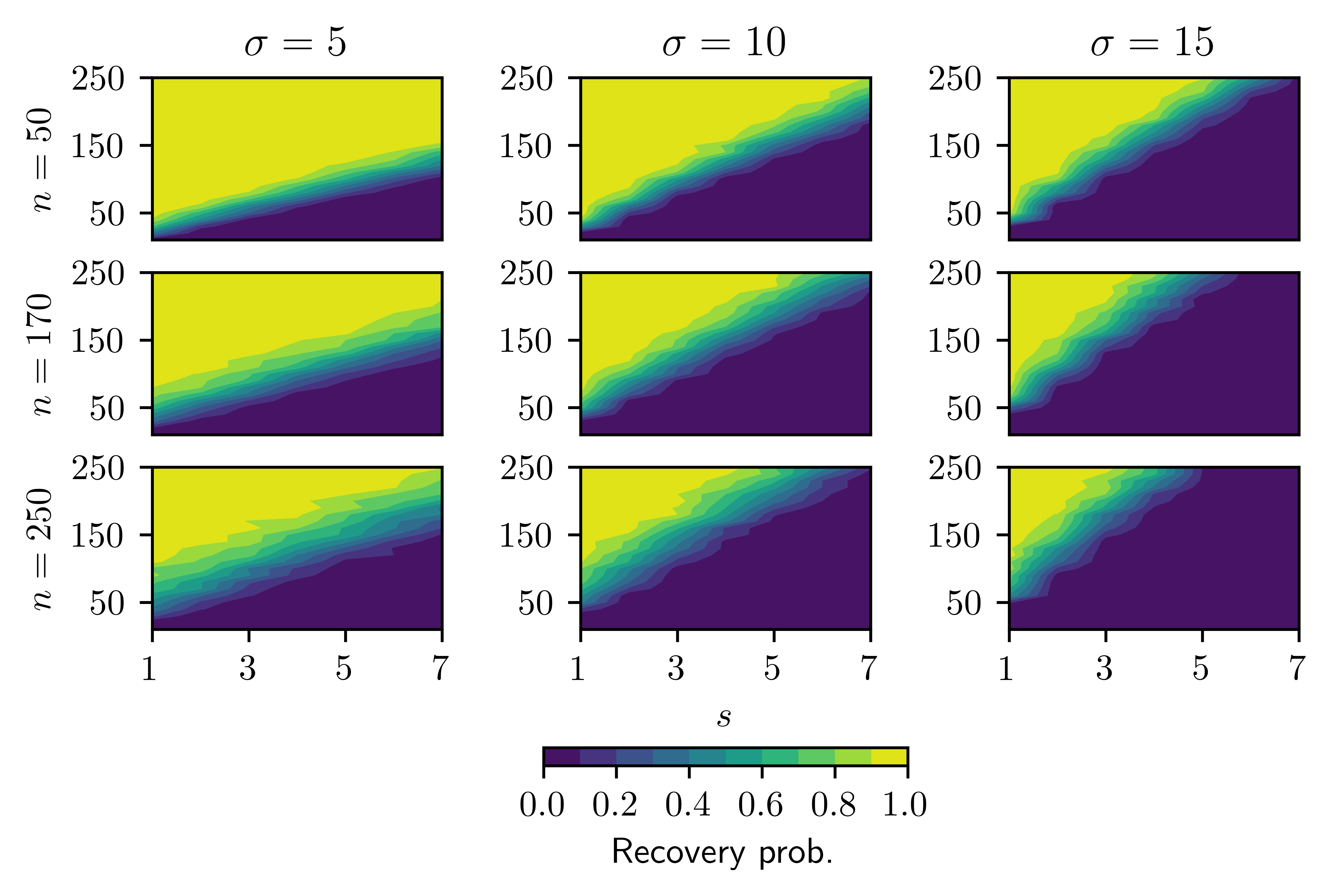
Figure 2: Recovery probability plots over $s=1,2,\dots,7$ and $\mu=10,20,\dots,250$ for different values of $n$ and $\sigma$.

By a simple visual inspection, we see that the number of measurements needed for successful recovery scales linearly with $s$ across all sparsities and values for $n$. We furthermore see that the dependence on $n$ is relatively mild.

To go further, we do a logistic regression of the empirical distributions against the values of

$$\lambda_{a}=\frac{\mu}{s^{a}\sigma\log(n)+C_{a}s\log(\mu)},$$

for $a=1$ and $a=2$ (we use the sklearn-package to do so). For each value of $a$, we manually tune the value $C_{a}>0$ to obtain the best fit. Indeed, the data fits much better to $\lambda_{1}$ than to $\lambda_{2}$ – the logistic loss for the former is $0.217$, and $0.40$ for the latter. A plot of the empirical probabilites against the values of $\lambda_{a}$, together with the logistic fit, for the two values of $a$ are shown in Figure 3.

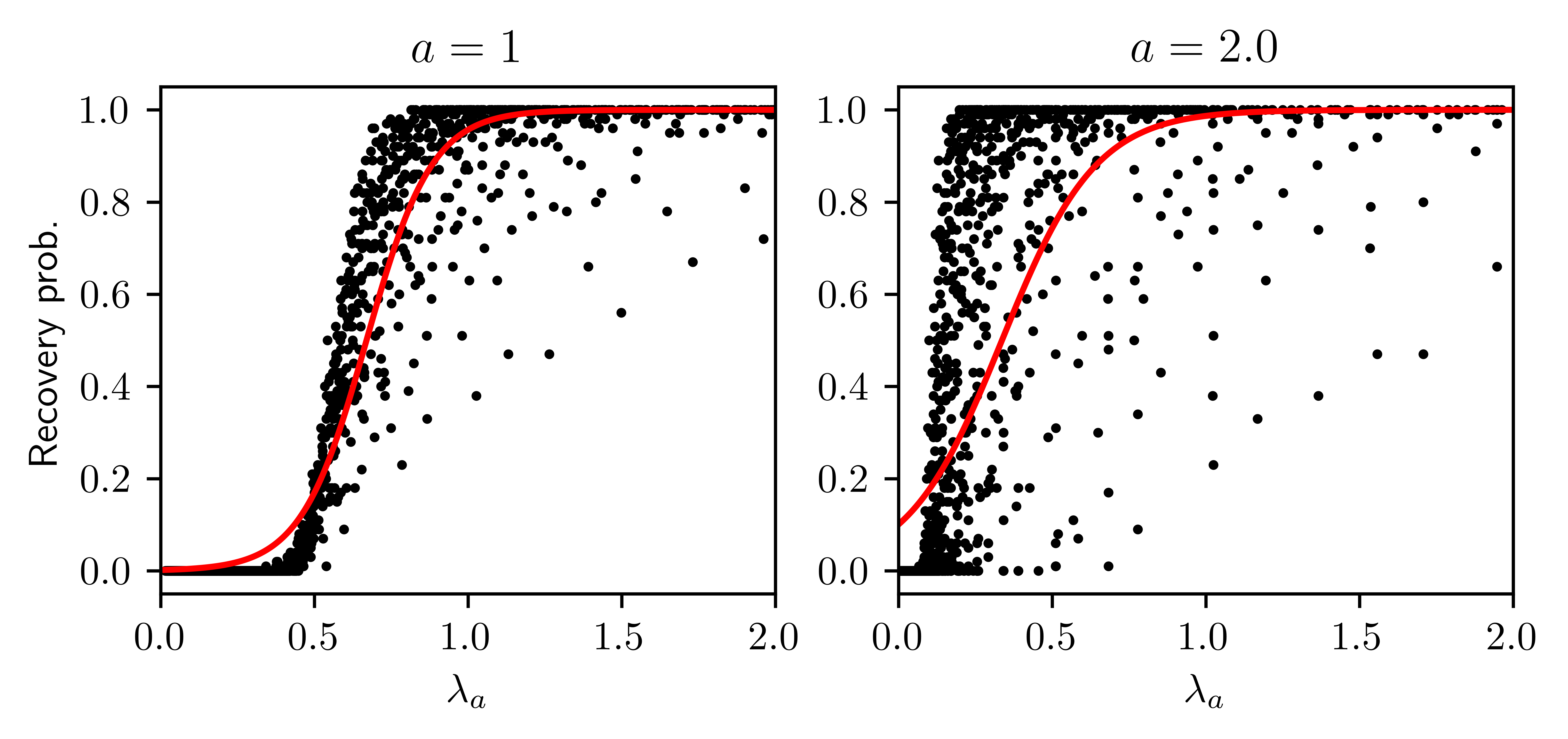
Figure 3: The empirical recovery probabilities and fitted logistic curves for the first set of experiments, i.e. $n=50,170,350$, $s=1,\dots,7$ and $\sigma=5,10,15$. Only datapoints with $\lambda_{a}\leq 2.0$ are displayed.

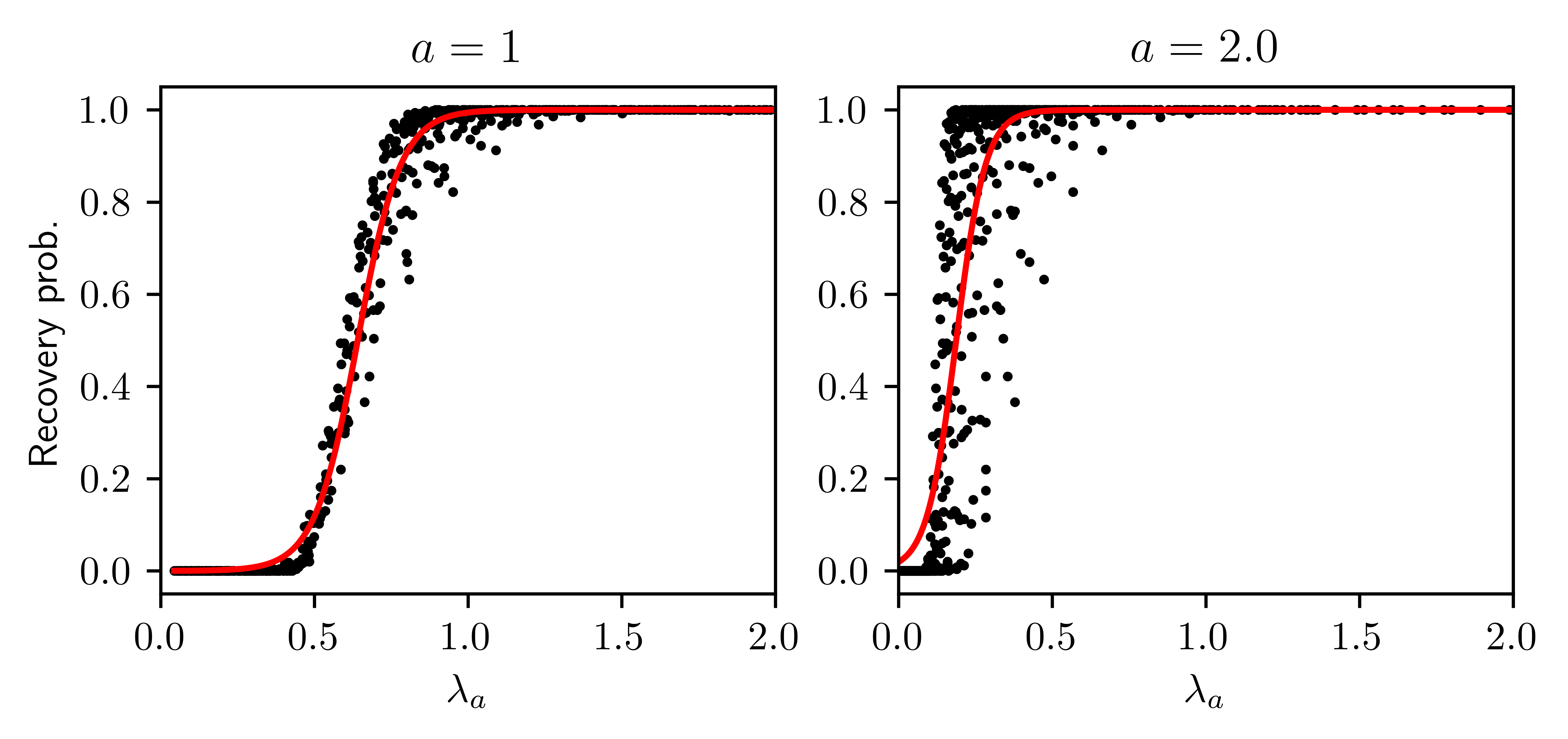
Figure 4: The empirical recovery probabilities and fitted logistic curves for the second set of experiments, i.e. $n=50$ $s=3,\dots,7$ and $\sigma=3,\dots,7$. Only datapoints with $\lambda_{a}\leq 2.0$ are displayed.

We repeat the last experiment for $n=50$, and both $\sigma$ and $s$ ranging between $3$ and $7$, performing $500$ experiments per data point. Now, the data even more points to $a=1$ being the correct model - the logistic loss for $a=1$ is now $0.148$ for the best $C_{a}$-value, whereas it is $0.27$ for $a=2$. The empirical success probabilitites and the fitted logistic curve are plotted against $\lambda_{a}$ in Figure 4.

We conclude that our experiments clearly suggest that the $s^{2}$-scaling is not reflective of the empirical performance of the HiHTP algorithm.

Acknowledgement

AF acknowledges support from the Wallenberg AI, Autonomous Systems and Software Program (WASP) funded by the Knut and Alice Wallenberg Foundation, and CHAIR. GW is supported by the German Science Foundation (DFG) under grants 598/7-1, 598/7-2, 598/8-1, 598/8-2 and the 6G research cluster (6g-ric.de) supported by the German Ministry of Education and Research (BMBF).

References

- [1] W. U. Bajwa, J. Haupt, A. M. Sayeed, and R. Nowak, “Compressed channel sensing: A new approach to estimating sparse multipath channels,” Proceedings of the IEEE, vol. 98, no. 6, pp. 1058–1076, 2010.
- [2] M. Kech and F. Krahmer, “Optimal injectivity conditions for bilinear inverse problems with applications to identifiability of deconvolution problems,” SIAM Journal on Applied Algebra and Geometry, vol. 1, pp. 20–37, 2017.
- [3] Y. Li, K. Lee, and Y. Bresler, “Identifiability and stability in blind deconvolution under minimal assumptions,” IEEE Trans. Inf. Th., vol. 63, pp. 4619–4633, 2017.
- [4] P. Netrapalli, P. Jain, and S. Sanghavi, “Phase retrieval using alternating minimization,” IEEE Trans. Sign. Proc., vol. 63, pp. 4814–4826, 2015.
- [5] K. Lee, Y. Li, M. Junge, and Y. Bresler, “Stability in blind deconvolution of sparse signals and reconstruction by alternating minimization,” in International Conference on Sampling Theory and Applications (SampTA), 2015, pp. 158–162.
- [6] ——, “Blind recovery of sparse signals from subsampled convolution,” IEEE Trans. Inf. Th., vol. 63, pp. 802–821, 2016.
- [7] S. Foucart, “Hard thresholding pursuit: an algorithm for compressive sensing,” SIAM Journal on Numerical Analysis, vol. 49, pp. 2543–2563, 2011.
- [8] D. Needell and J. A. Tropp, “Cosamp: Iterative signal recovery from incomplete and inaccurate samples,” Applied and computational harmonic analysis, vol. 26, pp. 301–321, 2009.
- [9] X. Li, S. Ling, T. Strohmer, and K. Wei, “Rapid, robust, and reliable blind deconvolution via nonconvex optimization,” Applied and computational harmonic analysis, vol. 47, pp. 893–934, 2019.
- [10] A. Ahmed, B. Recht, and J. Romberg, “Blind deconvolution using convex programming,” IEEE Trans. Inf. Th., vol. 60, pp. 1711–1732, 2013.
- [11] S. Ling and T. Strohmer, “Blind deconvolution meets blind demixing: Algorithms and performance bounds,” IEEE Trans. Inf. Th., vol. 63, pp. 4497–4520, 2017.
- [12] P. Jung, F. Krahmer, and D. Stöger, “Blind demixing and deconvolution at near-optimal rate,” IEEE Trans. Inf. Th., vol. 64, pp. 704–727, 2018.
- [13] S. Ling and T. Strohmer, “Self-calibration and biconvex compressive sensing,” Inverse Problems, vol. 31, p. 115002, sep 2015. [Online]. Available: https://doi.org/10.1088%2F0266-5611%2F31%2F11%2F115002
- [14] A. Flinth, “Sparse blind deconvolution and demixing through -minimization.” Advances in Computational Mathematics, vol. 44, 2018.
- [15] Y. Chen, J. Fan, B. Wang, and Y. Yan, “Convex and nonconvex optimization are both minimax-optimal for noisy blind deconvolution under random designs,” Journal of the American Statistical Association, pp. 1–11, 2021. [Online]. Available: https://doi.org/10.1080/01621459.2021.1956501
- [16] S. Foucart, R. Gribonval, L. Jacques, and H. Rauhut, “Jointly low-rank and bisparse recovery: Questions and partial answers,” Analysis and Applications, vol. 18, pp. 25–48, 2020.
- [17] M. Magdon-Ismail, “NP-hardness and inapproximability of sparse PCA,” Inf. Proc. Lett., vol. 126, pp. 35–38, Oct. 2017. [Online]. Available: http://www.sciencedirect.com/science/article/pii/S002001901730100X
- [18] S. O. Chan, D. Papailliopoulos, and A. Rubinstein, “On the approximability of sparse PCA,” in PMLR, vol. 49, Jun. 2016, pp. 623–646. [Online]. Available: http://proceedings.mlr.press/v49/chan16.html
- [19] M. Brennan and G. Bresler, “Optimal average-case reductions to sparse PCA: From weak assumptions to strong hardness,” Arxiv e-prints, Feb. 2019. [Online]. Available: http://arxiv.org/abs/1902.07380
- [20] H. Eisenmann, F. Krahmer, M. Pfeffer, and A. Uschmajew, “Riemannian thresholding methods for row-sparse and low-rank matrix recovery,” arXiv preprint arXiv:2103.02356, 2021.
- [21] K. Lee, Y. Wu, and Y. Bresler, “Near-optimal compressed sensing of a class of sparse low-rank matrices via sparse power factorization,” IEEE Trans. Inf. Th., vol. 64, pp. 1666–1698, 2017.
- [22] S. Bahmani and J. Romberg, “Near-optimal estimation of simultaneously sparse and low-rank matrices from nested linear measurements,” Information and Inference: A Journal of the IMA, vol. 5, pp. 331–351, 2016.
- [23] P. Sprechmann, I. Ramirez, G. Sapiro, and Y. Eldar, “Collaborative hierarchical sparse modeling,” in 2010 44th Annual Conference on Information Sciences and Systems (CISS), 2010, pp. 1–6.
- [24] J. Friedman, T. Hastie, and R. Tibshirani, “A note on the group lasso and a sparse group lasso,” Preprint, 2010, arXiv: 1001.0736.
- [25] P. Sprechmann, I. Ramirez, G. Sapiro, and Y. C. Eldar, “C-HiLasso: A collaborative hierarchical sparse modeling framework,” IEEE Trans. Sig. Proc., vol. 59, pp. 4183–4198, 2011.
- [26] N. Simon, J. Friedman, T. Hastie, and R. Tibshirani, “A sparse-group Lasso,” J. Comp. Graph. Stat., vol. 22, pp. 231–245, 2013.
- [27] J. Eisert, A. Flinth, B. Groß, I. Roth, and G. Wunder, “Hierarchical compressed sensing,” arXiv preprint arXiv:2104.02721, 2021.
- [28] I. Roth, M. Kliesch, A. Flinth, G. Wunder, and J. Eisert, “Reliable recovery of hierarchically sparse signals for gaussian and kronecker product measurements,” IEEE Transactions on Signal Processing, vol. 68, pp. 4002–4016, 2020.
- [29] R. G. Baraniuk, V. Cevher, M. F. Duarte, and C. Hegde, “Model-based compressive sensing,” IEEE Transactions on information theory, vol. 56, no. 4, pp. 1982–2001, 2010.
- [30] G. Wunder, I. Roth, R. Fritschek, B. Groß, and J. Eisert, “Secure massive iot using hierarchical fast blind deconvolution,” in 2018 IEEE Wireless Communications and Networking Conference Workshops (WCNCW). IEEE, 2018, pp. 119–124.
- [31] G. Wunder, S. Stefanatos, A. Flinth, I. Roth, and G. Caire, “Low-overhead hierarchically-sparse channel estimation for multiuser wideband massive mimo,” IEEE Transactions on Wireless Communications, vol. 18, pp. 2186–2199, April 2019.
- [32] A. Flinth, B. Groß, I. Roth, J. Eisert, and G. Wunder, “Hierarchical isometry properties of hierarchical measurements,” Appl. Harm. Comp. Anal, vol. 58, pp. 27–49, 2021.
- [33] E. J. Candès, “The restricted isometry property and its implications for compressed sensing,” Comptes Rendus Mathematique, vol. 346, no. 9, pp. 589–592, 2008. [Online]. Available: https://www.sciencedirect.com/science/article/pii/S1631073X08000964
- [34] R. Vershynin, High-Dimensional Probability. An Introduction with Applications in Data Science. Cambridge University Press, 2018.
- [35] G. Jagatap and C. Hedge, “Phase retrieval using structured sparsity: A sample efficient algorithmic framework,” stat, vol. 1050, p. 18, 2017.
- [36] G. Wang, L. Zhang, G. B. Giannakis, M. Akçakaya, and J. Chen, “Sparse phase retrieval via truncated amplitude flow,” IEEE Transactions on Signal Processing, vol. 66, pp. 479–491, 2017.
- [37] Z. Liu, S. Ghosh, and J. Scarlett, “Towards sample-optimal compressive phase retrieval with sparse and generative priors,” arXiv preprint arXiv:2106.15358, 2021.
- [38] M. Soltanolkotabi, “Structured signal recovery from quadratic measurements: Breaking sample complexity barriers via nonconvex optimization,” IEEE Trans. Inf. Th., vol. 65, pp. 2374–2400, 2019.
- [39] J.-F. Cai, J. Li, X. Lu, and J. You, “Sparse signal recovery from phaseless measurements via hard thresholding pursuit,” arXiv preprint arXiv:2005.08777, 2020.
- [40] F. Krahmer, S. Mendelson, and H. Rauhut, “Suprema of chaos processes and the restricted isometry property,” Communications on Pure and Applied Mathematics, vol. 67, pp. 1877–1904, 2014. [Online]. Available: https://onlinelibrary.wiley.com/doi/abs/10.1002/cpa.21504
- [41] M. Talagrand, The generic chaining. Upper and Lower Bounds of Stochastic Processes. Springer, 2005.
- [42] H. Rauhut, J. Romberg, and J. A. Tropp, “Restricted isometries for partial random circulant matrices,” Applied and Computational Harmonic Analysis, vol. 32, pp. 242–254, 2012. [Online]. Available: https://www.sciencedirect.com/science/article/pii/S1063520311000649
- [43] S. Dirksen, “Tail bounds via generic chaining,” Electronic Journal of Probability, vol. 20, pp. 1–29, 2015.
- [44] A. Böttcher and B. Silbermann, Introduction to Large Truncated Toeplitz Matrices. New York, NY: Springer New York, 1999. [Online]. Available: https://doi.org/10.1007/978-1-4612-1426-7_6
- [45] S. Foucart and H. Rauhut, A Mathematical Introduction to Compressive Sensing. Birkhäuser, 2013.
- [46] R. Okuta, Y. Unno, D. Nishino, S. Hido, and C. Loomis, “Cupy: A numpy-compatible library for nvidia gpu calculations,” in Proceedings of Workshop on Machine Learning Systems (LearningSys) in The Thirty-first Annual Conference on Neural Information Processing Systems (NIPS), 2017. [Online]. Available: http://learningsys.org/nips17/assets/papers/paper_16.pdf