The hadron pair forward-backward asymmetry in the electron positron annihilation process

Abstract

The forward-backward asymmetry is an important measurable quantity which can enable independent determination of the neutral-current couplings of fermions. In this paper, we extend the definition of the asymmetry from the partonic level to the hadronic level by calculating this asymmetry of the hadron pair in the semi-inclusive electron position annihilation process. Semi-inclusive implies that a back-to-back jet is also measured in addition to the hadron pair. Due to the limitation of the factorization theorem, we calculate this process up to leading order twist-4 level by applying the collinear expansion formalism. After obtaining the differential cross section, we calculate the forward-backward asymmetries and show them in terms of the corresponding di-hadron fragmentation functions. Di-hadron fragmentation functions are introduced to describe the hadron pair productions in the fragmentation process. With available parameterization of the functions, we present a numerical estimation of the forward-backward asymmetry. On the flip side, measurements of the forward-backward asymmetry would give strict restrictions of parameterizations of the di-hadron fragmentation functions. We also present a numerical estimation of the twist-4 di-hadron fragmentation functions in order to illustrate their contributions.

Keywords: forward-backward asymmetry, electron position annihilation

I Introduction

The spontaneously broken electroweak (EW) theory and the color gauge theory or quantum chromodynamics (QCD) are two basic components of the Standard Model (SM) which has achieved great success in describing the elementary particles and their interactions. Since the left- and right-handed fermions in the EW theory live in different representations of the fundamental gauge group, they have different couplings for the gauge bosons. As for $Z^{0}$, the difference leads to an asymmetry in the angular distribution of positively and negatively charged fermions (leptons and quarks) produced in $Z^{0}$ decays. This asymmetry, known as the forward-backward asymmetry Wu:1984ik ; Marshall:1988bk ; Langacker:1995eqb ; ALEPH:2005ab , depends on the weak mixing angle and can enable independent determinations of the neutral-current couplings of these fermions. Asymmetries for known fermions have definite distributions with respect to center-of-mass energy. They can be measured with very precision at the $Z^{0}$ pole. Therefore, it is more interesting to calculate the asymmetries for a certain produced hadron or hadron pair in the $Z^{0}$ decays. The difficulty in describing the weak interactions of quarks lies in the description of the quark fragmentation process. Thanks to the asymptotic freedom of QCD, the fragmentation process can be studied in the factorization theorem (see, e.g., Refs. Amati:1978wx ; Ellis:1978ty ; Collins:1989gx ). Factorization theorem tells that measurable quantities, e.g. cross section, can be separated by the calculable hard parts from the non-perturbative soft parts. If only the fragmentation process is taken into consideration, the non-perturbative soft parts are usually factorized as fragmentation functions (FFs) and/or di-hadron fragmentation functions (DiFFs). Quantities therefore can be expressed in terms of FFs and/or DiFFs in the annihilation and other fragmentation processes.

The discussion of the forward-backward asymmetry for a single certain hadron is available in Ref. Yang:2022mmh . In this paper, we consider the asymmetry for a hadron pair in the semi-inclusive electron positron annihilation process. The hadron pair is described by the DiFFs which were first introduced to describe the hadron pair production in a fragmenting jet at leading twist level in refs. Bianconi:1999cd ; Bianconi:1999uc and extended to the twist-3 level in Ref. Bacchetta:2003vn . DiFFs are assumed to be universal and can be factorized in high energy reactions. By extracting from the two-jet events in the electron positron annihilation process Boer:2003ya ; Bacchetta:2008wb ; Courtoy:2012ry ; Matevosyan:2018icf , they can be used to study the nucleon structures in the framework of collinear factorization Bacchetta:2002ux ; Bacchetta:2004it ; Bacchetta:2011ip ; Pisano:2015wnq . Recent measurement of the invariant-mass dependence DiFF can be found in Ref. Belle:2017rwm . DiFFs are also considered to be strongly related to the jet handedness and can be used to investigate the quark and/or gluon polarizations Boer:2003ya ; Pisano:2015wnq ; Metz:2016swz . Here we note that the hadron pair have two origins. First of all, the pair could come from a single parton which fragments into two hadrons. Second, two hadrons can also arise when the parton first splits into two partons with each of them afterwards fragmenting into a single hadron. The key to distinguish the two possible origins is the size of the hadron pair invariant mass. If the invariant mass is much smaller than the hard scale, we can parametrize the fragmentation process with the nonperturbative DiFFs. Otherwise, we fall back to the convolution of two single-hadron FFs. For the first case, the DiFFs is similar to FFs and they have the same evolution equations Metz:2016swz ; deFlorian:2003cg ; Ceccopieri:2007ip . For the second case, a splitting term should be added into the evolution equation. We do not consider this case in this paper.

Since factorization beyond leading order for twist-4 terms is unclear, we limit ourselves by leading order calculations in this paper. In other words, the calculations are carried out at leading order twist-4 by applying the collinear expansion formalism Ellis:1982wd ; Ellis:1982cd ; Qiu:1990xxa ; Qiu:1990xy . This will greatly simplify the systematic calculation of higher twist contributions. The detailed calculations for the hadron pair production electron positron process by one of us can be found in Yang:2022knp . In this paper we use the results and introduce the definition of the forward-backward asymmetry for the hadron pair and present these asymmetry results in terms of DiFFs. With the available parameterizations of the DiFF from the Monte Carlo simulation Courtoy:2012ry , we show numerical estimates for this asymmetry. We also present a numerical estimate of the twist-4 DiFFs in order to illustrate their contributions. To be explicit, we organize the rest of the paper as follows. In Sec. II, we first introduce the general definition of the forward-backward asymmetry of the fermion pair in the annihilation process and show some conventions used in this paper. We also present the results of the hadron pair production process obtained in Yang:2022knp . The explicit expressions of the forward-backward asymmetries in terms of DiFFs and numerical estimations are shown in Sec. III. A brief summary is finally given in Sec. IV.

II The differential cross section

II.1 The forward-backward asymmetry

A simple exercise for the fermion pair production in the electron positron annihilation process is to calculate the muon pair production process. By considering the EW theory, the tree level differential cross section of this process can be written as

$$\frac{d\sigma}{d\cos\theta}=\frac{\pi\alpha_{em}^{2}}{2Q^{2}} \bigg{\{}\chi\left[c_{1}^{e}c_{1}^{\mu}\left(1+\cos^{2}\theta\right)+2c_{3}^{e}c_{3}^{\mu}\cos\theta\right]$$

$$+ \chi_{int}\left[c_{V}^{e}c_{V}^{\mu}\left(1+\cos^{2}\theta\right)+2c_{A}^{e}c_{A}^{\mu}\cos\theta\right]$$

$$+ e_{q}^{2}\left(1+\cos^{2}\theta\right)\bigg{\}},$$ (1)

where $\theta$ is the scattering angle in the lepton center-of-mass frame or the gauge boson rest frame, $\alpha_{em}=e^{2}/4\pi$ is the fine structure constant and $Q^{2}=q^{2}=(l+l^{\prime})^{2}$.

$$\chi=\frac{Q^{4}}{\left[(Q^{2}-M_{Z}^{2})^{2}+\Gamma_{Z}^{2}M_{Z}^{2}\right]\sin^{4}2\theta_{W}},$$ (2)

$$\chi_{int}=-\frac{2e_{q}Q^{2}(Q^{2}-M_{Z}^{2})}{\left[(Q^{2}-M_{Z}^{2})^{2}+\Gamma_{Z}^{2}M_{Z}^{2}\right]\sin^{2}2\theta_{W}},$$ (3)

where $M_{Z}$ and $\Gamma_{Z}$ are respectively the mass and decay width of $Z$-boson, $\theta_{W}$ is the weak mixing angle. $c_{1}^{e}=(c_{V}^{e})^{2}+(c_{A}^{e})^{2}$ and $c_{3}^{e}=2c_{V}^{e}c_{A}^{e}$, $c_{V}^{e}$ and $c_{A}^{e}$ are defined in the weak interaction current $J_{\mu}(x)=\bar{\psi}(x)\Gamma_{\mu}\psi(x)$ where $\Gamma_{\mu}=\gamma_{\mu}(c_{V}^{e}-c_{A}^{e}\gamma^{5})$. Similar notations are also used for muon and quarks where we use a superscripts $\mu$ and $q$ to replace $e$.

The forward-backward asymmetry in the angular distribution of positively and negatively charged fermions is defined as

$$A_{FB}=\frac{\int_{0}^{1}d\sigma_{\theta}d\cos\theta-\int_{-1}^{0}d\sigma_{\theta}d\cos\theta}{\int_{-1}^{1}d\sigma_{\theta}d\cos\theta},$$ (4)

where $d\sigma_{\theta}=d\sigma/d\cos\theta$ is the differential cross section given in Eq. (1). Using the definition in Eq. (4) and the differential cross section in Eq. (1), we obtain

$$A^{f}_{FB}=\frac{3(\chi c_{3}^{e}c_{3}^{f}+\chi_{int}c_{A}^{e}c_{A}^{f})}{4(e_{f}^{2}+\chi c_{1}^{e}c_{1}^{f}+\chi_{int}c_{V}^{e}c_{V}^{f})},$$ (5)

where superscript $f$ denotes fermions (muon and quarks) and $e_{f}$ is the corresponding electric charge. In the following context, we extend the results to the hadron pair production process. We note that the definition of the forward-backward asymmetry given in Eq. (4) will be slightly modified for calculating that for hadron pairs. It will be shown in Sec. III.

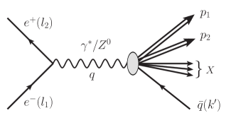
Figure 1: Illustrating diagram for the $e^{+}+e^{-}\to h_{1}+h_{2}+\bar{q}+X$ process.

II.2 The formalism

To be explicit, we label the tree-level semi-inclusive electron positron annihilation process as

$$e^{+}+e^{-}\to q+\bar{q}\to h_{1}+h_{2}+\bar{q}+X$$ (6)

where $\bar{q}$ denotes an antiquark that corresponds to a jet of hadrons and $h_{1},h_{2}$ denote outgoing hadrons fragmented from $q$ in experiments, see Fig. 1. The differential cross section of this process is given by

$$d\sigma= \frac{\alpha_{em}^{2}}{2\pi^{2}sQ^{4}}A_{r}L^{r}_{\mu\nu}(l_{1},l_{2})W_{r}^{\mu\nu}(p_{1},p_{2},k^{\prime})\frac{d^{3}p_{1}}{2E_{1}}\frac{d^{3}p_{2}}{2E_{2}}\frac{d^{3}k^{\prime}}{2\pi 2E_{k}},$$ (7)

where $s=Q^{2}=q^{2}$ with $q=l_{1}+l_{2}$, $l_{1},l_{2}$ are momenta of the leptons, $p_{1},p_{2}$ are momenta of the outgoing hadrons.The symbol $r$ can be $\gamma\gamma$, $ZZ$ and $\gamma Z$, for electromagnetic (EM), weak and interference terms, respectively. A summation over $r$ is understood, i.e., the total cross section is given by

$$d\sigma=d\sigma^{ZZ}+d\sigma^{\gamma Z}+d\sigma^{\gamma\gamma}.$$ (8)

$A_{r}$’s are defined as

$$A_{\gamma\gamma}=e_{q}^{2}, A_{ZZ}=\chi, A_{\gamma Z}=\chi_{int}.$$ (9)

The leptonic tensors for different cases are respectively given by

$$L^{\gamma\gamma}_{\mu\nu}(l_{1},l_{2})=l_{1\mu}l_{2\nu}+l_{1\nu}l_{2\mu}-(1_{l}\cdot l_{2})g_{\mu\nu},$$ (10)

$$L^{ZZ}_{\mu\nu}(l_{1},l_{2})=c_{1}^{e}\left[l_{1\mu}l_{2\nu}+l_{1\nu}l_{2\mu}-(1_{l}\cdot l_{2})g_{\mu\nu}\right]+ic_{3}^{e}\varepsilon_{\mu\nu l_{1}l_{2}},$$ (11)

$$L^{\gamma Z}_{\mu\nu}(l_{1},l_{2})=c_{V}^{e}\left[l_{1\mu}l_{2\nu}+l_{1\nu}l_{2\mu}-(1_{l}\cdot l_{2})g_{\mu\nu}\right]\!+\!ic_{V}^{e}\varepsilon_{\mu\nu l_{1}l_{2}},$$ (12)

where coefficients $c_{1,3}^{e}$ have been introduced in the previous subsection. The corresponding hadronic tensor are given by

$$W_{\gamma\gamma}^{\mu\nu}= \sum_{X}\delta(q-p_{1}-p_{2}-k^{\prime}-p_{X})\langle 0|J^{\mu}_{\gamma\gamma}(0)|p_{1},p_{2},k^{\prime},X\rangle\langle p_{1},p_{2},k^{\prime},X|J^{\nu}_{\gamma\gamma}(0)|0\rangle,$$ (13)

$$W_{ZZ}^{\mu\nu}= \sum_{X}\delta(q-p_{1}-p_{2}-k^{\prime}-p_{X})\langle 0|J^{\mu}_{ZZ}(0)|p_{1},p_{2},k^{\prime},X\rangle\langle p_{1},p_{2},k^{\prime},X|J^{\nu}_{ZZ}(0)|0\rangle,$$ (14)

$$W_{\gamma Z}^{\mu\nu}= \sum_{X}\delta(q-p_{1}-p_{2}-k^{\prime}-p_{X})\langle 0|J^{\mu}_{ZZ}(0)|p_{1},p_{2},k^{\prime},X\rangle\langle p_{1},p_{2},k^{\prime},X|J^{\nu}_{\gamma\gamma}(0)|0\rangle,$$ (15)

where $J^{\mu}_{\gamma\gamma}(0)=\bar{\psi}(0)\gamma^{\mu}\psi(0)$ and $J^{\mu}_{ZZ}(0)=\bar{\psi}(0)\Gamma^{\mu}\psi(0)$. Although, we have shown EM, weak and interference terms for both the leptonic and hadronic tensors, we only present calculations of the weak interaction in the following context for simplicity. Other cases can be obtained in the similar way or by changing $c_{1},c_{3}$ into $1,0$ and $c_{V},c_{A}$ for EM and interference cases, respectively.

In describing the hadron pair production in the electron positron annihilation process, following the previous conventions Bianconi:1999cd ; Bianconi:1999uc , we define $p_{h}=p_{1}+p_{2}$, $R=(p_{1}-p_{2})/2$ and introduce the frame where momenta can be parameterized in the following forms:

$$q=Q(1,0,0,0),$$ (16)

$$l_{1}=\frac{Q}{2}(1,-\sin\theta,0,-\cos\theta),$$ (17)

$$p_{h}=(E_{h},0,0,p_{z}),$$ (18)

$$R=(E_{r},|R_{T}|\cos\phi_{r},|R_{T}|\sin\phi_{r},R_{z}),$$ (19)

$$k^{\prime}=(E_{k},|k^{\prime}_{T}|\cos\phi_{k},|k^{\prime}_{T}|\sin\phi_{k},k^{\prime}_{z}).$$ (20)

We also introduce the following standard variables used in this paper,

$$z=\frac{2p_{h}\cdot q}{Q^{2}}=\frac{2p_{1}\cdot q}{Q^{2}}+\frac{2p_{2}\cdot q}{Q^{2}}=z_{1}+z_{2},$$ (21)

$$\xi=\frac{z_{1}}{z}=1-\frac{z_{2}}{z}.$$ (22)

In terms of the variables above, the phase space factor can be rewritten as

$$\frac{d^{3}p_{1}}{2E_{1}}\frac{d^{3}p_{2}}{2E_{2}}\frac{d^{3}k^{\prime}}{2E_{k}}=\frac{\pi}{8}zQ^{2}dzdyd\phi_{r}dM_{h}^{2}d\xi\frac{dk^{\prime}_{z}}{2E_{k}}d^{2}k^{\prime}_{T}.$$ (23)

Here we have used $d\Omega=2dyd\phi_{L}=4\pi dy$ where $y=p_{h}\cdot l_{1}/p_{h}\cdot q$, $\phi_{L}$ is the angle of lepton with respect to $p_{h}$. The differential cross section therefore can be rewritten as

$$\frac{d\sigma}{dzdyd\phi_{r}M_{h}^{2}d\xi d^{2}k^{\prime}_{T}}=\frac{\alpha_{em}^{2}z}{16\pi Q^{4}}\chi L_{\mu\nu}(l_{1},l_{2})W^{\mu\nu}(p_{h},k^{\prime}_{T}).$$ (24)

Here the $k^{\prime}_{T}$-dependent hadronic tensor is defined by integrating over $dk_{z}^{\prime}$,

$$W^{\mu\nu}(p_{h},k^{\prime}_{T})=\int\frac{dk^{\prime}_{z}}{2\pi 2E_{k}}W^{\mu\nu}(p_{h},k^{\prime}).$$ (25)

In the leptons center-of-mass frame $|k_{T}|=|k^{\prime}_{T}|$, the hadronic tensor therefore can also be seen as a function of $k_{T}$.

II.3 The cross section at twist-4

Without repeating the tedious mathematical calculations which can be found in Yang:2022knp , we here only write down the result of the differential cross section for simplicity. The complete expression for the weak interaction process at tree level twist-4 is given by

$$[d\sigma] =\frac{\alpha_{em}^{2}\chi}{8\pi Q^{2}}\Bigg{\{}T_{1}(y)\left(D_{1}-\kappa^{2}_{M}\frac{D_{4q}}{z}\right)+T_{2}(y)k_{TM}R_{TM}\sin(\phi_{r}-\phi_{k})\left(G^{\perp}_{1}-\kappa^{2}_{M}\frac{G_{4q}}{z}\right)$$

$$-2\kappa_{M}\left[T_{3}(y)k_{TM}\cos\phi_{k}D^{\perp}+T_{3}(y)R_{TM}\cos\phi_{r}D^{\sphericalangle}\right]$$

$$-2\kappa_{M}\left[T_{4}(y)k_{TM}\sin\phi_{k}G^{\perp}+T_{4}(y)R_{TM}\sin\phi_{r}G^{\sphericalangle}\right]$$

$$+4\kappa_{M}^{2}\Big{[}2c_{1}^{e}c_{1}^{q}B(y)\frac{D_{3}}{z}+2c_{1}^{e}c_{3}^{q}B(y)k_{TM}R_{TM}\sin(\phi_{r}-\phi_{k})\frac{G_{3}}{z}-T_{1}(y)\mathrm{Re}D_{-3dd}\Big{]}$$

$$-4\kappa_{M}^{2}c_{1}^{e}c_{1}^{q}B(y)\Big{[}k_{TM}^{2}\cos 2\phi_{k}\mathrm{Re}D^{\perp}_{-3d}+R_{TM}^{2}\cos 2\phi_{r}\mathrm{Re}D^{\sphericalangle}_{-3d}+k_{TM}R_{TM}\cos(\phi_{r}+\phi_{k})\mathrm{Re}D^{\times}_{-3d}\Big{]}$$

$$-4\kappa_{M}^{2}c_{1}^{e}c_{3}^{q}B(y)\Big{[}k_{TM}^{2}\sin 2\phi_{k}\mathrm{Im}D^{\perp}_{-3d}+R_{TM}^{2}\sin 2\phi_{r}\mathrm{Im}D^{\sphericalangle}_{-3d}+k_{TM}R_{TM}\sin(\phi_{r}+\phi_{k})\mathrm{Im}D^{\times}_{-3d}\Big{]}\Bigg{\}},$$ (26)

where $[d\sigma]=d\sigma/dzdyd\phi_{r}dM_{h}^{2}d\xi d^{2}k^{\prime}_{T}$. We also used $k_{TM}=|k_{T}|/M_{h}$, $R_{TM}=|R_{T}|/M_{h}$ and

$$T_{1}(y)=2c_{1}^{e}c_{1}^{q}A(y)-c_{3}^{e}c_{3}^{q}C(y),$$ (27)

$$T_{2}(y)=2c_{1}^{e}c_{3}^{q}A(y)-c_{3}^{e}c_{1}^{q}C(y),$$ (28)

$$T_{3}(y)=c_{1}^{e}c_{1}^{q}C(y)D(y)+c_{3}^{e}c_{3}^{q}D(y),$$ (29)

$$T_{4}(y)=c_{1}^{e}c_{3}^{q}C(y)D(y)-c_{3}^{e}c_{1}^{q}D(y)$$ (30)

with $A(y)=\frac{1}{2}-y+y^{2},B(y)=2y(1-y),C(y)=1-2y$ and $D(y)=\sqrt{y(1-y)}$ to simplify the expression. The twist suppression factor $\kappa_{M}$ is defined as $\kappa_{M}=M_{h}/Q$. Contributions from four-quark correlator which are labeled with subscript $4q$ are involved in Eq. (26), e.g, $D_{4q}/z$. As for the EM and the interference cases, $T_{i}(i=1,2,3,4)$ are respectively reduced as

$$T^{em}_{1}(y)=2A(y),$$ (31)

$$T^{em}_{2}(y)=0,$$ (32)

$$T^{em}_{3}(y)=C(y)D(y),$$ (33)

$$T^{em}_{4}(y)=0,$$ (34)

$$T^{int}_{1}(y)=2c_{V}^{e}c_{V}^{q}A(y)-c_{A}^{e}c_{A}^{q}C(y),$$ (35)

$$T^{int}_{2}(y)=2c_{V}^{e}c_{A}^{q}A(y)-c_{A}^{e}c_{V}^{q}C(y),$$ (36)

$$T^{int}_{3}(y)=c_{V}^{e}c_{V}^{q}C(y)D(y)+c_{A}^{e}c_{A}^{q}D(y),$$ (37)

$$T^{int}_{4}(y)=c_{V}^{e}c_{A}^{q}C(y)D(y)-c_{A}^{e}c_{V}^{q}D(y).$$ (38)

The kinematic factor $\chi$ should changes to $e_{q}^{2}$ and $\chi_{int}$ for EM and interference contributions, respectively. The total cross section is the sum of the EM, weak and interference terms, see Eq. (8).

III The results at twist-4

III.1 The forward-backward asymmetry

The forward-backward asymmetry which is introduced to describe the angle distribution of the fermions from $Z^{0}$ decays has been introduced in Sec. II. Here we redefine the asymmetry at the hadonic level to illustrate the angle distribution of the produced hadron pair in the electron positron annihilation process. Comparing to Eq. (4), we define the forward-backward asymmetry for a hadron pair as

$$A_{FB}=\frac{\int_{0}^{1}[d\sigma]d\cos\theta-\int_{-1}^{0}[d\sigma]d\cos\theta}{\int_{-1}^{1}[d\sigma]_{U}d\cos\theta},$$ (39)

where $[d\sigma]$ is the differential cross section of the scattering angle $\theta(\cos\theta)$ while $[d\sigma]_{U}$ denotes the azimuthally independent one. Instead of $\cos\theta$, the differential cross section is given in terms of $y$ in Eq. (26). It is then convenient to rewrite the forward-backward asymmetry $A_{FB}$ in the following form,

$$A_{FB}=\frac{\int_{1/2}^{1}(d\sigma)dy-\int_{0}^{1/2}(d\sigma)dy}{\int_{0}^{1}(d\sigma)_{U}dy},$$ (40)

where $(d\sigma)=d\sigma/dzdyd\phi_{r}dM_{h}^{2}d\xi d^{2}k^{\prime}_{T}$ and $(d\sigma)_{U}$ only includes azimuthally independent terms. Remember the differential cross section is a sum of the EM, weak and interference terms, see Eq. (8). Then we obtain the denominator:

$$\int^{1}_{0}(d\sigma)_{U}dy=\frac{\alpha_{em}^{2}}{12Q^{2}}\left(e_{q}^{2}+\chi c_{1}^{e}c_{1}^{q}+\chi_{int}c_{V}^{e}c_{V}^{q}\right)\tilde{D}_{1},$$ (41)

where $\tilde{D}_{1}=D_{1}-\kappa^{2}_{M}D_{4q}/z$.

Using the asymmetry definition in Eq. (40) and the corresponding differential cross section, we obtain 6 kinds of asymmetries, 2 of them are leading twist effects while 4 of them are twist-3 effects:

$$A_{FB} =\frac{3\left(\chi c_{3}^{e}c_{3}^{q}+\chi_{int}c_{A}^{e}c_{A}^{q}\right)\tilde{D}_{1}}{4\left(e_{q}^{2}+\chi c_{1}^{e}c_{1}^{q}+\chi_{int}c_{V}^{e}c_{V}^{q}\right)\tilde{D}_{1}},$$ (42)

$$A_{FB}^{kR,y} =\frac{3\left(\chi c_{3}^{e}c_{1}^{q}+\chi_{int}c_{A}^{e}c_{V}^{q}\right)\tilde{G}^{\perp}_{1}}{4\left(e_{q}^{2}+\chi c_{1}^{e}c_{1}^{q}+\chi_{int}c_{V}^{e}c_{V}^{q}\right)\tilde{D}_{1}},$$ (43)

$$A_{FB}^{k,x} =-k_{TM}\frac{\kappa_{M}\left(\chi c_{1}^{e}c_{1}^{q}+\chi_{int}c_{V}^{e}c_{V}^{q}\right)D^{\perp}}{2\left(e_{q}^{2}+\chi c_{1}^{e}c_{1}^{q}+\chi_{int}c_{V}^{e}c_{V}^{q}\right)\tilde{D}_{1}},$$ (44)

$$A_{FB}^{k,y} =-k_{TM}\frac{\kappa_{M}\left(\chi c_{1}^{e}c_{3}^{q}+\chi_{int}c_{V}^{e}c_{A}^{q}\right)G^{\perp}}{2\left(e_{q}^{2}+\chi c_{1}^{e}c_{1}^{q}+\chi_{int}c_{V}^{e}c_{V}^{q}\right)\tilde{D}_{1}},$$ (45)

$$A_{FB}^{r,x} =-R_{TM}\frac{\kappa_{M}\left(\chi c_{1}^{e}c_{1}^{q}+\chi_{int}c_{V}^{e}c_{V}^{q}\right)D^{\sphericalangle}}{2\left(e_{q}^{2}+\chi c_{1}^{e}c_{1}^{q}+\chi_{int}c_{V}^{e}c_{V}^{q}\right)\tilde{D}_{1}},$$ (46)

$$A_{FB}^{r,y} =-R_{TM}\frac{\kappa_{M}\left(\chi c_{1}^{e}c_{3}^{q}+\chi_{int}c_{V}^{e}c_{A}^{q}\right)G^{\sphericalangle}}{2\left(e_{q}^{2}+\chi c_{1}^{e}c_{1}^{q}+\chi_{int}c_{V}^{e}c_{V}^{q}\right)\tilde{D}_{1}},$$ (47)

where $\tilde{G}^{\perp}_{1}=G^{\perp}_{1}-\kappa^{2}_{M}G_{4q}/z$. Twist-4 asymmetries are suppressed at high energies, we do not show them here. We note that a summation of flavor $q$ is explicit in the numerator and in the denominator, respectively. This applies also to all the results presented in the following context. From the point of view of experimental measurement, it is convenient to consider contributions from the collinear DiFFs. If one integrates over $k_{T}$, only asymmetries shown in Eqs. (42), (46) and (47) are left.

Considering the low energy limit, forward-backward asymmetries shown above can be rewritten as

$$A_{FB} =\frac{3G_{F}Q^{2}c_{A}^{e}c_{A}^{q}\tilde{D}_{1}}{4\sqrt{2}e_{q}\pi\alpha_{em}\tilde{D}_{1}},$$ (48)

$$A_{FB}^{kR,y} =\frac{3G_{F}Q^{2}c_{A}^{e}c_{V}^{q}\tilde{G}^{\perp}_{1}}{4\sqrt{2}e_{q}\pi\alpha_{em}\tilde{D}_{1}},$$ (49)

$$A_{FB}^{k,x} =-k_{TM}\kappa_{M}\frac{G_{F}Q^{2}c_{V}^{e}c_{V}^{q}D^{\perp}}{2\sqrt{2}e_{q}\pi\alpha_{em}\tilde{D}_{1}},$$ (50)

$$A_{FB}^{k,y} =-k_{TM}\kappa_{M}\frac{G_{F}Q^{2}c_{V}^{e}c_{A}^{q}G^{\perp}}{2\sqrt{2}e_{q}\pi\alpha_{em}\tilde{D}_{1}},$$ (51)

$$A_{FB}^{r,x} =-R_{TM}\kappa_{M}\frac{G_{F}Q^{2}c_{V}^{e}c_{V}^{q}D^{\sphericalangle}}{2\sqrt{2}e_{q}\pi\alpha_{em}\tilde{D}_{1}},$$ (52)

$$A_{FB}^{r,y} =-R_{TM}\kappa_{M}\frac{G_{F}Q^{2}c_{V}^{e}c_{A}^{q}G^{\sphericalangle}}{2\sqrt{2}e_{q}\pi\alpha_{em}\tilde{D}_{1}},$$ (53)

where $G_{F}=g^{2}/4\sqrt{2}M_{W}^{2}=e^{2}/\sqrt{2}M_{Z}^{2}\sin^{2}2\theta_{W}$, is the Fermi constant.

To have an intuitive impression of the hadron forward-backward asymmetry shown above, we present the numerical values of $A_{FB}$ in Fig. 2. We do not show other asymmetries due to lack of proper parameterizations. Parameterizations of $D_{1}(z,M_{h},Q^{2})$ are taken from ref. Courtoy:2012ry in which only $u,d,s$ and $c$ quarks are considered. The QCD evolution of the DiFF starts from $Q^{2}=1GeV$ and is limited at leading order Metz:2016swz ; deFlorian:2003cg ; Ceccopieri:2007ip . Invariant mass $M_{h}$ is chosen as $0.5GeV$. As a contrast, the asymmetries for quarks are shown by dashed lines while asymmetries for the produced hadron pair are shown by solid lines. From Fig. 2, we see the forward-backward asymmetry of the hadron pair is insensitive to the momentum fraction $z$ but can be distinguished from that of the quarks.

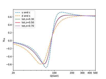
Figure 2: The forward-backward asymmetry for $A_{FB}$. Dashed lines show asymmetries for quarks. Solid lines show asymmetries for produced hadron pairs with different momentum fraction $z$. Here $M_{h}=0.5GeV$.

III.2 Estimation of the twist-4 DiFFs

In this paper, our calculations are shown at twist-4 level. In order to estimate the contributions from the twist-4 DiFFs, we introduce the ratio of the twist-4 DiFFs to the leading twist DiFF. For simplicity, we consider

$$[d\sigma] =\frac{\alpha_{em}^{2}\chi}{8Q^{2}}\Bigg{\{}T_{1}(y)\left(D_{1}-\kappa^{2}_{M}\frac{D_{4q}}{z}\right)+4\kappa_{M}^{2}\Big{[}2c_{1}^{e}c_{1}^{q}B(y)\frac{D_{3}}{z}-T_{1}(y)\mathrm{Re}D_{-3dd}\Big{]}\Bigg{\}},$$ (54)

where $k_{T}$- and $R_{T}$-dependent terms are neglected. In terms of twist-4 contribution factor or the ratio $\alpha$, we have

$$[d\sigma] =\frac{\alpha_{em}^{2}\chi}{8Q^{2}}\left[T_{1}(y)D_{1}\left(1+\kappa^{2}_{M}\alpha\right)-T_{1}(y)\kappa^{2}_{M}\frac{D_{4q}}{z}\right],$$ (55)

where

$$\alpha=4\frac{2c_{1}^{e}c_{1}^{q}B(y)D_{3}-zT_{1}(y)\mathrm{Re}D_{-3dd}}{zT_{1}(y)D_{1}}.$$ (56)

We next need to find the relations between $D_{3},\mathrm{Re}D_{-3dd}$ and $D_{1}$. Since $D_{1}$ and $D_{3}$ can be obtained by calculating the traces from the decomposition of the correlation function, using $\not{k}=k^{+}\not{\bar{n}}+k^{-}\not{n}+\not{k}_{T}$, we finally have

$$D_{3}=-\frac{z^{2}k_{T}^{2}}{2M_{h}^{2}}D_{1}.$$ (57)

By using the rough approximation $g=0$, i.e., neglecting the contribution from gluons, we calculate the quark-gluon-gluon-quark correlator and obtain Yang:2022knp

$$\big{(}\hat{\Xi}^{(2)}_{\rho\sigma}+\gamma^{0}\hat{\Xi}^{(2){\dagger}}_{\sigma\rho}\gamma^{0}\big{)}|_{g=0}=k_{T\rho}k_{T\sigma}z^{2}\frac{\partial}{\partial z}\hat{\Xi}^{(0)}|_{g=0}.$$ (58)

Inserting the decomposition of the quark-j-gluon-quark correlator into Eq. (58) and neglecting the T-odd functions (e.g., $G_{3dd}$), we obtain

$$2\mathrm{Re}D_{3dd}=\frac{z^{2}k_{T}^{2}}{2M_{h}^{2}}\frac{\partial}{\partial z}D_{1}.$$ (59)

Therefore the $\alpha$ can be rewritten as

$$\alpha=zk_{TM}^{2}\left[\frac{\partial\ln T_{1}(y)D_{1}}{\partial\ln z}+\frac{4c_{1}^{e}c_{1}^{q}B(y)D_{1}}{T_{1}(y)D_{1}}\right].$$ (60)

With the parametrization of $D_{1}$ used in the previous subsection, we show a rough estimation of the twist-4 contribution factor $\alpha$ in Fig. 3. We can see that the ratio $\alpha$ is sensitive to the invariant mass of the hadron pair for $z>0.3$ and the twist-4 DiFFs have approximately the same order of magnitude as the leading twist DiFF $D_{1}$. Higher twist suppressions come from the factor $\kappa_{M}$ rather than the higher twist parton functions. However, for $z<0.3$, the twist-4 DiFFs are one order of magnitude smaller than the leading twist DiFF $D_{1}$.

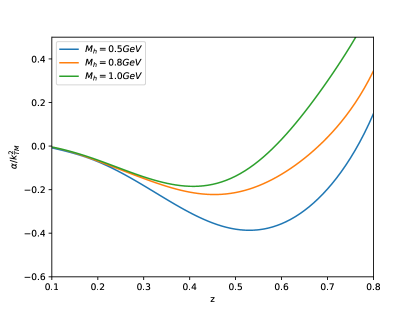
Figure 3: A rough estimation of the twist-4 contribution factor $\alpha/k_{TM}^{2}$ as a function of $z$ at $Q=M_{Z}$ with different $M_{h}$.

III.3 The azimuthal asymmetries

From Eq. (26), we can see there are sets of azimuthal modulations which can be measured in experiments and used to extract the corresponding DiFFs. We show the results for completeness in the following.

To clarify our calculations we first present the definition of the azimuthal asymmetries, e.g.

$$\langle\sin\phi_{k}\rangle=\frac{\int[d\sigma]\sin\phi_{k}d\phi_{k}}{\int[d\sigma]d\phi_{k}}.$$ (61)

Other asymmetries can be defined in the similar way, we do not show them here. According to the definition, we write down all the azimuthal asymmetries. The leading twist asymmetry is given by

$$\langle\sin(\phi_{r}-\phi_{k})\rangle_{2}=k_{TM}R_{TM}\frac{\chi T_{2}(y)G^{\perp}_{1}}{2\chi T_{1}(y)D_{1}}.$$ (62)

Here subscript $2$ denotes the leading twist. The twist-4 correction of the leading twist asymmetry in Eq. (62) in the numerator is $\kappa_{M}^{2}\left(-T_{2}(y)G_{4q}+8c_{1}^{e}c_{3}^{q}B(y)G_{3}\right)/z$.

There are four twist-3 azimuthal asymmetries which are given by

$$\langle\cos\phi_{k}\rangle_{3}=-\kappa_{M}k_{TM}\frac{\chi T_{3}(y)D^{\perp}}{z\chi T_{1}(y)D_{1}},$$ (63)

$$\langle\cos\phi_{r}\rangle_{3}=-\kappa_{M}R_{TM}\frac{\chi T_{3}(y)D^{\sphericalangle}}{z\chi T_{1}(y)D_{1}},$$ (64)

$$\langle\sin\phi_{k}\rangle_{3}=-\kappa_{M}k_{TM}\frac{\chi T_{4}(y)G^{\perp}}{z\chi T_{1}(y)D_{1}},$$ (65)

$$\langle\sin\phi_{r}\rangle_{3}=-\kappa_{M}R_{TM}\frac{\chi T_{4}(y)G^{\sphericalangle}}{z\chi T_{1}(y)D_{1}},$$ (66)

where subscript $3$ denotes the twist-3. There are six twist-4 azimuthal asymmetries which are given by

$$\langle\cos 2\phi_{k}\rangle_{4}=-\kappa^{2}_{M}k^{2}_{TM}\frac{2\chi c_{1}^{e}c_{1}^{q}B(y)\mathrm{Re}D_{-3d}^{\perp}}{z\chi T_{1}(y)D_{1}},$$ (67)

$$\langle\cos 2\phi_{r}\rangle_{4}=-\kappa^{2}_{M}R^{2}_{TM}\frac{2\chi c_{1}^{e}c_{1}^{q}B(y)\mathrm{Re}D_{-3d}^{\sphericalangle}}{z\chi T_{1}(y)D_{1}},$$ (68)

$$\langle\sin 2\phi_{k}\rangle_{4}=-\kappa^{2}_{M}k^{2}_{TM}\frac{2\chi c_{1}^{e}c_{3}^{q}B(y)\mathrm{Im}D_{-3d}^{\perp}}{z\chi T_{1}(y)D_{1}},$$ (69)

$$\langle\sin 2\phi_{r}\rangle_{4}=-\kappa^{2}_{M}R^{2}_{TM}\frac{2\chi c_{1}^{e}c_{3}^{q}B(y)\mathrm{Im}D_{-3d}^{\sphericalangle}}{z\chi T_{1}(y)D_{1}},$$ (70)

$$\langle\cos(\phi_{r}+\phi_{k})\rangle_{4}=\kappa^{2}_{M}k_{TM}R_{TM}\frac{2\chi c_{1}^{e}c_{1}^{q}B(y)\mathrm{Re}D_{-3d}^{\times}}{z\chi T_{1}(y)D_{1}},$$ (71)

$$\langle\sin(\phi_{r}+\phi_{k})\rangle_{4}=\kappa^{2}_{M}k_{TM}R_{TM}\frac{2\chi c_{1}^{e}c_{3}^{q}B(y)\mathrm{Im}D_{-3d}^{\times}}{z\chi T_{1}(y)D_{1}},$$ (72)

where subscript $4$ denotes the twist-4.

IV Summary

The forward-backward asymmetry is an important measurable quantity which can be used to determine the neutral-current couplings. In this paper, we extend the definition of the asymmetry from the partonic level to the hadronic level by calculating this asymmetry of the hadron pair in the semi-inclusive electron position annihilation process. The production of the hadron pair is described by the DiFFs. Semi-inclusive implies that a back-to-back jet is also measured in addition to the hadron pair. We first calculate the cross section according to the collinear expansion method. It provides explicit expressions of the hadronic tensor at twist-4 level and the cross section can be easily obtained. We calculate the leading twist and twist-3 forward-backward asymmetries and present the numerical estimates at leading twist with available parametrizations. We find that the forward-backward asymmetry of the hadron pair is insensitive to the momentum fraction $z$ but can be distinguished from that of the quarks. We also show a rough estimation of the twist-4 DiFFs. We find that the twist-4 DiFFs are one order of magnitude smaller than the leading twist DiFF $D_{1}$ in the $z<0.3$ region. However, for $z>0.3$, the twist-4 DiFFs have approximately the same order of magnitude as the leading twist DiFF $D_{1}$. Azimuthal asymmetries are also shown for completeness.

References

- (1) S. L. Wu, Phys. Rept. 107, 59-324 (1984) doi:10.1016/0370-1573(84)90033-4
- (2) R. Marshall, Z. Phys. C 43, 607 (1989) doi:10.1007/BF01550939
- (3) P. Langacker, “Precision tests of the standard electroweak model,” doi:10.1142/1927
- (4) S. Schael et al. [ALEPH, DELPHI, L3, OPAL, SLD, LEP Electroweak Working Group, SLD Electroweak Group and SLD Heavy Flavour Group], Phys. Rept. 427, 257-454 (2006) doi:10.1016/j.physrep.2005.12.006 [arXiv:hep-ex/0509008 [hep-ex]].
- (5) D. Amati, R. Petronzio and G. Veneziano, Nucl. Phys. B 140, 54-72 (1978) doi:10.1016/0550-3213(78)90313-9
- (6) R. K. Ellis, H. Georgi, M. Machacek, H. D. Politzer and G. G. Ross, Nucl. Phys. B 152, 285-329 (1979) doi:10.1016/0550-3213(79)90105-6
- (7) J. C. Collins, D. E. Soper and G. F. Sterman, Adv. Ser. Direct. High Energy Phys. 5, 1 (1989) doi:10.1142/97898145032660001 [hep-ph/0409313].
- (8) W. Yang and C. Li, Phys. Rev. D 106, no.3, 036016 (2022) doi:10.1103/PhysRevD.106.036016 [arXiv:2205.04068 [hep-ph]].
- (9) A. Bianconi, S. Boffi, R. Jakob and M. Radici, Phys. Rev. D 62, 034008 (2000) doi:10.1103/PhysRevD.62.034008 [arXiv:hep-ph/9907475 [hep-ph]].
- (10) A. Bianconi, S. Boffi, R. Jakob and M. Radici, Phys. Rev. D 62, 034009 (2000) doi:10.1103/PhysRevD.62.034009 [arXiv:hep-ph/9907488 [hep-ph]].
- (11) A. Bacchetta and M. Radici, Phys. Rev. D 69, 074026 (2004) doi:10.1103/PhysRevD.69.074026 [arXiv:hep-ph/0311173 [hep-ph]].
- (12) D. Boer, R. Jakob and M. Radici, Phys. Rev. D 67, 094003 (2003) [erratum: Phys. Rev. D 98, no.3, 039902 (2018)] doi:10.1103/PhysRevD.67.094003 [arXiv:hep-ph/0302232 [hep-ph]].
- (13) A. Bacchetta, F. A. Ceccopieri, A. Mukherjee and M. Radici, Phys. Rev. D 79, 034029 (2009) doi:10.1103/PhysRevD.79.034029 [arXiv:0812.0611 [hep-ph]].
- (14) A. Courtoy, A. Bacchetta, M. Radici and A. Bianconi, Phys. Rev. D 85, 114023 (2012) doi:10.1103/PhysRevD.85.114023 [arXiv:1202.0323 [hep-ph]].
- (15) H. H. Matevosyan, A. Bacchetta, D. Boer, A. Courtoy, A. Kotzinian, M. Radici and A. W. Thomas, Phys. Rev. D 97, no.7, 074019 (2018) doi:10.1103/PhysRevD.97.074019 [arXiv:1802.01578 [hep-ph]].
- (16) A. Bacchetta and M. Radici, Phys. Rev. D 67, 094002 (2003) doi:10.1103/PhysRevD.67.094002 [arXiv:hep-ph/0212300 [hep-ph]].
- (17) A. Bacchetta and M. Radici, Phys. Rev. D 70, 094032 (2004) doi:10.1103/PhysRevD.70.094032 [arXiv:hep-ph/0409174 [hep-ph]].
- (18) A. Bacchetta, A. Courtoy and M. Radici, Phys. Rev. Lett. 107, 012001 (2011) doi:10.1103/PhysRevLett.107.012001 [arXiv:1104.3855 [hep-ph]].
- (19) S. Pisano and M. Radici, Eur. Phys. J. A 52, no.6, 155 (2016) doi:10.1140/epja/i2016-16155-5 [arXiv:1511.03220 [hep-ph]].
- (20) R. Seidl et al. [Belle], Phys. Rev. D 96, no.3, 032005 (2017) doi:10.1103/PhysRevD.96.032005 [arXiv:1706.08348 [hep-ex]].
- (21) A. Metz and A. Vossen, Prog. Part. Nucl. Phys. 91, 136-202 (2016) doi:10.1016/j.ppnp.2016.08.003 [arXiv:1607.02521 [hep-ex]].
- (22) D. de Florian and L. Vanni, Phys. Lett. B 578, 139-149 (2004) doi:10.1016/j.physletb.2003.10.047 [arXiv:hep-ph/0310196 [hep-ph]].
- (23) F. A. Ceccopieri, M. Radici and A. Bacchetta, Phys. Lett. B 650, 81-89 (2007) doi:10.1016/j.physletb.2007.04.065 [arXiv:hep-ph/0703265 [hep-ph]].
- (24) R. K. Ellis, W. Furmanski and R. Petronzio, Nucl. Phys. B 207, 1 (1982).
- (25) R. K. Ellis, W. Furmanski and R. Petronzio, Nucl. Phys. B 212, 29 (1983).
- (26) J. -w. Qiu and G. F. Sterman, Nucl. Phys. B 353, 105 (1991).
- (27) J. -w. Qiu and G. F. Sterman, Nucl. Phys. B 353, 137 (1991).
- (28) W. Yang, Eur. Phys. J. C 82, no.8, 741 (2022) doi:10.1140/epjc/s10052-022-10698-y