Generalizing over Long Tail Concepts for Medical Term Normalization

Abstract

Medical term normalization consists in mapping a piece of text to a large number of output classes. Given the small size of the annotated datasets and the extremely long tail distribution of the concepts, it is of utmost importance to develop models that are capable to generalize to scarce or unseen concepts. An important attribute of most target ontologies is their hierarchical structure. In this paper we introduce a simple and effective learning strategy that leverages such information to enhance the generalizability of both discriminative and generative models. The evaluation shows that the proposed strategy produces state-of-the-art performance on seen concepts and consistent improvements on unseen ones, allowing also for efficient zero-shot knowledge transfer across text typologies and datasets.

1 Introduction

Term normalization is the task of mapping a variety of natural language expressions to specific concepts in a dictionary or an ontology. It is a key component for information processing systems, and it is extensively used in the medical domain. In this context, term normalization is often used to map reported adverse events (AEs) related to a drug to a medical ontology, such as MedDRA (Brown et al., 1999). This is a challenging task, due to the high variability of natural language input (i.e., from the informality of social media and conversational transcripts to the formality of medical and legal reports) and the high cardinality and long tail distribution of the output concepts. AEs are usually mappable to different levels of the same ontology: low-level concepts, which are closer to layman terms, and higher level concepts, which encompass the meaning of multiple low-level concepts. In MedDRA, these two sets of concepts are called Lowest Level Terms (LLT), and Preferred Terms (PT) respectively; both of them have a very high cardinality (48,713 for LLT and 24,571 for PT, in MedDRA version 23.1). The following are examples of AEs, with their corresponding LLTs and PTs:

AE	LLT	PT
feel like crap	feeling unwell	malaise
weak knees	weakness	asthenia
zap me of all energy	loss of energy	asthenia

Currently this problem is addressed with large pretrained language models (Gonzalez-Hernandez et al., 2020), finetuned on medical term normalization datasets, such as SMM4H (Gonzalez-Hernandez et al., 2020) or CADEC (Karimi et al., 2015). However, these datasets contain maximum 5,000 samples, distributed on a few PT/LLT classes, and with a long tail distribution (see Figure 1). Due to the size and distribution of these datasets, the resulting models usually perform well on examples that are seen in the training, but struggle to generalize on rare or unseen samples.

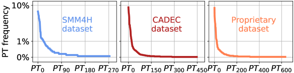
Figure 1: Long tail distribution of PTs in the datasets used for this paper.

To improve the generalization capabilities of the models on long tail concepts, in this paper, we suggest to leverage the hierarchical nature of the medical ontology to enrich the large language models with domain knowledge before finetuning on a given training set. Extensive experimental evaluation on three different datasets shows that the proposed strategy can be successfully applied to various model typologies, and it consistently outperforms other mainstream learning strategies, showing generalization capabilities not only across the long tail distribution, but also across text typologies and datasets. The code and resources needed to replicate our experiments and test our learning strategy are publicly available.

2 Related Work

Medical term normalization is generally regarded as either a classification or a ranking problem (Yuan et al., 2022). In the former case, a neural architecture encodes the term into a hidden representation and outputs a distribution over the classes (Limsopatham and Collier, 2016; Tutubalina et al., 2018; Niu et al., 2019), but this is difficult to scale to ontologies containing thousands of concepts, due to the absence of comprehensive datasets. In the ranking approach, on the other hand, the goal is to rank concepts by their similarity to the input term (Leaman et al., 2013; Li et al., 2017; Sung et al., 2020): a system is trained on binary classification, where terms and matching concepts are the positive samples, while terms and non-matching concepts are the negative ones. The raw output of the model is then used to rank the concepts.

Recent work successfully combined the two approaches. Ziletti et al. (2022) presented a system mixing a BERT-based classifier (Devlin et al., 2019) and a zero/few-shot learning method to incorporate label semantics in the input instances (Halder et al., 2020), showing improved performance in single model and in ensemble settings.

Finally, systems like CODER (Yuan et al., 2022) and SapBERT (Liu et al., 2021) introduced novel contrastive pretraining strategies that leverage UMLS to improve the medical embeddings of BERT-based models. While SapBERT leverages self-alignment methods, CODER maximizes the similarities between positive term-term pairs and term-relation-term triples and it claimed state-of-the-art results on several tasks, including zero-shot term normalization. Another recent work by Zhang et al. (2021) introduced an even more extensive pretraining procedure, based on self-supervision and a combination of the traditional masked language modelling with contrastive losses . The strategy proved to be extremely effective for medical entity linking, a kind of term normalization which makes use of the full original context (instead of using only the AE).

3 Proposed Learning Strategy: OP+FT

Dataset	Total Samples	Train Samples	Test Samples	%out Samples	Unique PTs
SMM4H	1,442	868 ±06	574 ±06	12.49 ±0.94	274
CADEC	5,866	3,540 ±21	2,326 ±21	4.65 ±0.41	488
PROP	4,453	2,658 ±65	1,796 ±65	10.02 ±0.79	634

Table 1: Dimensions of the datasets, reporting the average figures over the three train/test splits (± std), as well as the number of unique PT terms contained in each dataset.

Let’s consider a target ontology (e.g. MedDRA v23.1) containing two sets of concepts $\mathit{PT}=\{p_{i}\}$ and the $\mathit{LLT}=\{\ell_{i}\}$. The ontology is structured so that every $\ell_{i}$ has only one parent $p_{j}$: $\mathit{parent}(\ell_{i})=p_{j}$, but each $p_{j}$ can be parent of many $\ell_{i}$. Given a set of Adverse Events $\mathit{AE}=\{a_{i}\}$, every $a_{i}$ can be univocally mapped to a $p_{j}$: $\mathit{norm}(a_{i})=p_{j}$.

Our objective is to train a large language model $\mathcal{M}$ to encode $\mathit{norm}$: given a sample $(a_{i},p_{j})$, such that $\mathit{norm}(a_{i})=p_{j}$, we want $\mathcal{M}(a_{i})=p_{j}$.

We propose a learning strategy based on the hierarchical structure of the ontology, composed of two steps: Ontology Pretraining and Finetuning.

During the first step, we expose the language model $\mathcal{M}$ to all possible output classes $p_{j}$ by leveraging the intrinsic hierarchical relation between LLT and PT. Specifically, we use the $\mathit{parent}$ relation to create a new set of training samples from the ontology, pairing each $\ell_{i}$ to its parent concept $p_{j}$. In the case of MedDRA, the new set of samples contains 48,713 $(\ell_{i},p_{j})$ pairs, where each $p_{j}$ appears multiple times, associated with different $\ell_{i}$. For example the PT “asthenia” will appear in the samples (weakness, asthenia), and (loss of energy, asthenia). As LLTs are more informal than PTs, the language model $\mathcal{M}$ can be pretrained on this new set of data to gain general knowledge about all the target classes. This pretraining set is highly similar to our target dataset ($\mathcal{M}(a_{i})=p_{j}$), increasing the model transfer capability. We call this process “Ontology Pretraining” (OP).

The second step consists in finetuning (FT) an OP model on a specific term normalization dataset, which maps every AE $a_{i}$ to the corresponding PT $p_{j}$. This step is crucial because the OP model lacks specific knowledge about the natural language style of real-world samples. Finetuning will also exploit the dataset sample distribution to boost the model’s accuracy on the specific set of $p_{j}$ in the training set. Note that the FT step can also be applied to a regular model without OP, resulting in a regular finetuning.

We hypothesize that the combination of OP+FT to a discriminative or a generative language model $\mathcal{M}$ will improve its performance on seen concepts in the training set, while making it more generalizable to long tail and unseen concepts.

4 Experimental Setting

4.1 Datasets

To investigate the performance of our learning strategy, we used three English datasets for MedDRA term normalization, with different writing styles.

SMM4H (Gonzalez-Hernandez et al., 2020). Public dataset for the challenge SMM4H 2020 - Task 3, AE normalization. It contains 2,367 tweets, 1,212 of which report AEs with highly informal language, mapped to a PT/LLT.

CADEC (Karimi et al., 2015). Public dataset containing 1,250 posts from the health forum “AskaPatient”, containing user-reported AEs mapped to a PT/LLT. The language is informal, but still more medically precise than SMM4H.

PROP. Proprietary dataset provided by Bayer Pharmaceuticals, containing 2,010 transcripts of phone-calls with healthcare professionals reporting their patients’ AEs, mapped to PTs. The language is more formal and medically accurate.

4.2 Data Preparation

All datasets were preprocessed to obtain samples containing only $(a_{i},p_{j})$ pairs. The samples in CADEC and SMM4H which were labelled with an $\ell_{i}\in\mathit{LLT}$ were re-labelled with $\mathit{parent}(\ell_{i})=p_{j}\in\mathit{PT}$, obtaining a uniform output space for all datasets containing only PT concepts.

Since the focus of this work is on the generalization capabilities of the models, it is important to test the models on different sets of unseen labels. For this reason, we created three random splits of train/test samples using a 60:40 proportion, instead of using the public fixed train/test split. Given a train and a test set, every test sample with label $p_{j}$ falls into one of the following categories:
– in, if $p_{j}$ is present in the training set;
– out, if $p_{j}$ is not present in the training set.

The most important set of samples to measure the generalization capabilities of the models is out.

Table 1 reports figures for the resulting datasets. CADEC and PROP contain the largest number of samples (5,866 and 4,453 respectively), while SMM4H is sensibly smaller, with only 1,442 samples. The largest datasets also contain the largest number of PTs: 488 for CADEC and 634 for PROP. SMM4H only contains 274 PTs instead. Most of the PTs are unique to one of the three datasets and do not appear in the other ones, making it impossible to gain a substantial advantage by combining them (see Appendix C). We observe that the percentage of out samples varies from 5% to 12%, with SMM4H being the most challenging dataset. The standard deviation is low, showing that the presence of 5–12% out samples is a characteristic of the specific dataset, resulting from its long tail PT distribution. Note also that the smaller the dataset, the higher the percentage of out samples in the test set.

4.3 Models

To test the proposed strategy and observe how it affects generalization, we selected different kinds of widely-adopted models. In particular, we compare PubMedBERT (Gu et al., 2020), Sci5 (Phan et al., 2021), GPT-2 (Radford et al., 2019), CODER (Yuan et al., 2022) and SapBERT (Liu et al., 2021).

PubMedBERT (PMB). It was chosen as an example of a BERT-based classifier due to its medical pretraining (PubMed articles) and strong performance in other medical tasks (Gu et al., 2020; Portelli et al., 2021; Scaboro et al., 2021, 2022).

GPT-2 and Sci5. GPT-2 was selected as an example of a general-purpose autoregressive language model for text generation, while Sci5 was chosen for its medical pretraining, performed on the same kind of texts as PMB. The models were trained to generate a PT, given an input prompt containing the adverse event.

CODER and SapBERT (SapB). To the best of our knowledge, CODER and SapBERT are some of the best dataset-agnostic models for medical term embeddings. They were both trained on the UMLS ontology (Bodenreider, 2004), which is a super-set of MedDRA, and tested on several term normalization datasets, showing promising results. Following both original papers, we use CODER and SapBERT to generate embeddings for $a_{i}$ and for all $p_{j}\in\mathit{PT}$. We then select as prediction the $p_{j}$ that minimizes the cosine similarity with $a_{i}$.

We also trained both models according to our proposed strategy. Both models were trained using the contrastive settings described in their paper and the respective codebases.

See Appendix A for training details for all models and B for more details on the contrastive training of CODER and SapBERT.

Performance is assessed with the Accuracy metric, but we also report the F1 Score in Appendix D, as it can give more insights when classes are unbalanced.

5 Experimental Results

In an ablation-study fashion, we compare the OP+FT learning strategy with its two components: OP and FT. Figure 2 contains the results for all the tested models and training strategies, and is organized as follows. We display a plot for each dataset, reporting the accuracy of the models on in samples ($\circ$), out samples ($\diamond$) and the whole test set ($\bullet$). The first column shows the performance of a basic CODER and SapBERT model without any additional training. We consider their accuracy on out ($\diamond$) as our generalization goal, and plot them as solid lines across the chart. The following three columns display the performance of all the models, trained with one of the learning strategies (FT, OP and OP+FT respectively). For tabular results, see Appendix D.

CODER and SapBERT on their own proved to be strong baselines across the three datasets. Looking at the first column, they reach 40–50% accuracy on CADEC and SMM4H (overall, in and out, see solid lines), and around 15–20% overall accuracy ($\bullet$) on PROP.

All learning strategies seemed to be ineffective on CODER: its performance (gray markers) remains roughly the same across all strategies (FT, OP or OP+FT). A possible explanation for this behaviour is that CODER embeddings are already in an optimal state according to the training objectives, as they have been trained on a very similar task. In fact, CODER generates predictions using the similarity between the embeddings, and the stable performance indicates that there were no drastic changes in the structure of the embedding space.

A clearer effect of the training strategies can be seen on SapBERT (lilac markers), although it is still limited when compared with the other models. SapBERT embeddings are probably more subject to adjustments compared to CODER because the latter was trained for significantly more steps and using more objective functions, leading to less-adaptable embeddings.

The following observations apply the other three models: PMB, GPT-2 and Sci5.

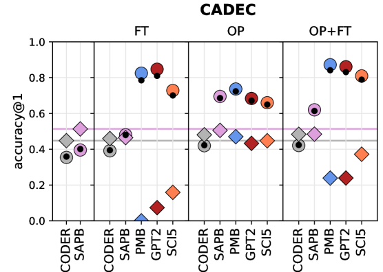
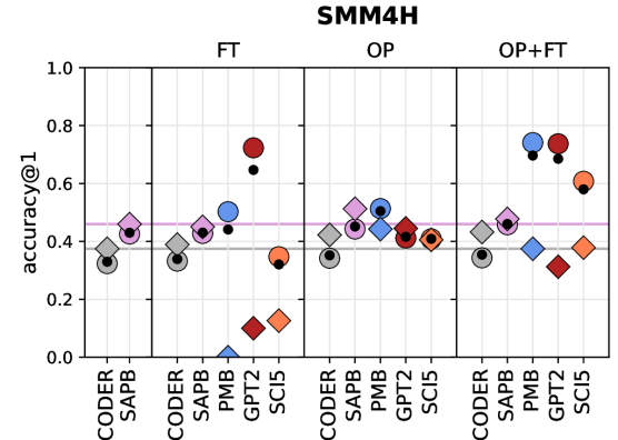
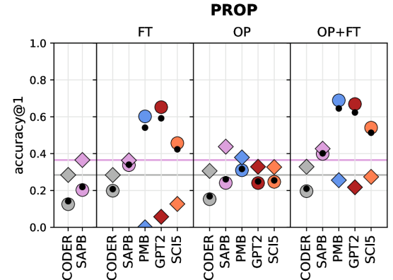
Figure 2: Accuracy of all models on the three datasets on in ($\circ$), out ($\diamond$) and all ($\bullet$) samples.

The FT strategy (second column), as expected, works really well for in ($\circ$) samples: on CADEC the in accuracy of all models is over to 80%, while it is close to 50% for the other two datasets. However, the out accuracy ($\diamond$) is lower than 20% in all cases (significantly lower than the solid line), and reaches 0% for PMB, showing that finetuning alone is not sufficient for classifiers to generalize on out samples in this setting.

The OP strategy (third column), brings the out accuracy of all models on pair with the CODER/SapBERT baselines, while the in/overall accuracy matches or surpasses them. Comparing OP with FT, we see that the overall accuracy ($\bullet$) of the model is generally lower for OP. However, the performance on out ($\diamond$) samples doubles for generative models, and jumps from 0 to  40% for PMB. This shows that the first step of our proposed learning strategy has the desired effect, as it improves the models’ understanding of all the output classes.

Finally, looking at the models trained with the OP+FT strategy (fourth column), we see that they outperform the FT ones on overall and in accuracy. The effect is particularly strong on the SMM4H dataset (cf. PMB FT, 44% and PMB OP+FT, 70%). At the same time, the performance on out ($\diamond$) samples remains similar to the OP models and close to the CODER baseline (gray solid line). The only exception is CADEC, where the performance on out is in-between the baseline and the accuracy with FT only. This shows that the proposed OP+FT learning strategy can successfully improve the generalization capabilities of various language models, while also improving their overall performance.

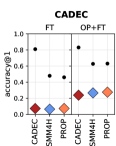
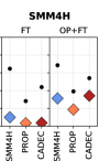
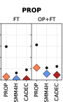
Figure 3: Cross-dataset accuracy for GPT-2 (FT and OP+FT) on out ($\diamond$) and all ($\bullet$) samples. One plot for each test dataset; the x-axis reports the training dataset.

We further test the generalization of OP+FT models in zero-shot, cross-dataset term normalization, normalizing the terms of each dataset with models that have been trained on one of the other two. Figure 3 shows the accuracy of GPT-2, with a plot for each test dataset, different training datasets on the x-axis, and one column for each learning strategy (FT or OP+FT). The behaviour of the other models is similar (see Appendix D). In all columns, we observe a drop in overall accuracy ($\bullet$) between the first data point and the following ones (e.g., cf. CADEC trained on CADEC and CADEC trained on SMM4H). However, this drop is larger for FT models than OP+FT ones (e.g., 35 vs. 20 points on CADEC). In addition, the out accuracy of OP+FT models remains high regardless of the training set. This shows that OP+FT models generalize better than FT models across-dataset. Note that generalization is still challenging when moving from a dataset with highly informal language to a formal one (see PROP trained on SMM4H).

6 Conclusions

In this paper, we shed some light on the importance of generalization for medical term normalization models. We showed that AE normalization models trained with traditional finetuning, despite showing high accuracy on leaderboards, have low generalization capabilities due to the long tail distribution of the target labels. Our proposed training strategy (OP+FT), which leverages the hierarchical structure of the ontology, outperforms traditional models, while also obtaining state-of-the-art results in generalization on out samples. This was also demonstrated in a zero-shot normalization setting. OP+FT showed improvements on discriminative and generative language models, while it seems to be less effective on models trained with contrastive losses. This promising technique could also be applied to other tasks with massive output spaces organized in a hierarchical manner.

Limitations

The proposed learning strategy was tested only for the task of medical term normalization (from adverse events to MedDRA concepts). However, it would be interesting to test its effectiveness on other term normalization tasks beyond MedDRA mapping and outside of the medical domain.

Even restricting the problem to medical term normalization, and using datasets with different text styles, we only focused on English texts. Medical ontologies such as MedDRA and UMLS are released in multiple languages, and the research community is moving towards multi-lingual approaches. In the future, we plan to extend this strategy to other languages (such as Spanish and Chinese) and to test the models’ capacity to perform crosslingual transfer in zero-shot scenarios.

Appendix A Training Specifications

Table 2 contains the specifics for the number of Ontology Pretraining (OP) and Finetuning (FT) used for all the selected models.

Model	OP epochs	FT epochs	OP+FT epochs
PMB	30	10	30  +	5
GPT-2	30	15	30  +	10
Sci5	40	15	40  +	8
CODER	50	20	50  +	15
SapBERT	30	15	30  +	10

Table 2: Further details about training parameters

Other model-related details:

• PMB A classification head (24,571 output classes) was added to the base model.

• GPT-2 Given a sample $(a_{i},p_{j})$, the input prompt for the model was "INPUT: $a$\nMEANING:". The model was trained to complete the sentence with $p_{j}$.

• Sci5 Given a sample $(a_{i},p_{j})$, the input prompt for the model was "normalize: $a$". The model was trained to respond with a string containing $p_{j}$.

• CODER/ SapBERT Following their original papers, we use CODER/SapBERT to normalize an AE $a$ as follows:

  $$\hat{p}=\mathop{\mathrm{argmax}}_{p\in P}\mathit{sim}(\mathcal{C}(a),\mathcal{C}(p))$$

  where $\mathit{sim}$ is a similarity measure (cosine, in our case), and $\mathcal{C}(\cdot)$ is the result of embedding a term with CODER/SapBERT. $\hat{p}$ is the predicted PT, which is compared with the actual one to evaluate the model.

Appendix B Sample Creation for Contrastive Training

B.1 CODER

CODER leverages on term-term pairs and term-relation-term triples for its contrastive training strategy. We create positive/negative samples for the term-term pairs using the AEs having equal/different PT, and term-relation-term triples connecting AEs whose PTs have the same $\mathit{parent}$.

For example, let’s consider the following $(a_{i},p_{j})$ samples, for which we also report $\mathit{parent}(p_{j})$:

$a_{i}$	$p_{j}$	$\mathit{parent}(p_{j})$
feel like crap	malaise	Asthenic conditions
weak knees	asthenia	Asthenic conditions
zap me of all energy	asthenia	Asthenic conditions

This will generate the following training samples for CODER:

• positive term-term:
  (weak knees, zap me of all energy)
  because they share the same $p_{j}$ “asthenia”

• negative term-term:
  (weak knees, feel like crap) and
  (zap me of all energy, feel like crap)
  because they are labelled with a different $p_{j}$ (“asthenia” vs “malaise”)

• positive term-relation-term:
  (weak knees, RO, feel like crap) and
  (zap me of all energy, RO, feel like crap),
  because their $p_{j}$ share the same $\mathit{parent}$ “Asthenic conditions”. RO stands for “Related Other”, one of the standard term relations defined in the UMLS ontology, and we use it to encode the relation “same granparent”.

This sample generation procedure is repeated for all samples in the three datasets (SMM4H, CADEC and PROP), as well as for the additional samples generated from MedDRA for the OP strategy.

B.2 SapBERT

SapBERT leverages on term-term synonym pairs, where the positive pairs belong to the same upper-level concept.

The finetuning script present in the GitHub repository requires a list of term pairs belonging to the same concept. In the the case of the three datasets (SMM4H, CADEC and PROP) we generate the terms pairs as $(\ell_{i},a_{j})$, where $\mathit{parent}(\ell_{i})=\mathit{norm}(a_{j})$. For the OP strategy, the samples are all possible pairs $(\ell_{i},\ell_{j})$, where $\mathit{parent}(\ell_{i})=\mathit{parent}(\ell_{j})$.

Appendix C Dataset Comparison

Most of the PTs present in the three datasets are unique to a specific dataset, making it really challenging to perform transfer learning from one to the other without dealing with long-tail and unseen concepts. The Venn diagram in Figure 4 shows the number of PT concepts in common between all the datasets. 706 PTs are unique to one of the three datasets, 276 are shared among at least two datasets, and only 98 appear in all three of them. Out of all the PTs in PROP, 64% are unique (410 out of 634) to this dataset alone, making it the most challenging to perform cross-dataset normalization on. The following most challenging datasets are CADEC (41% unique PTs) and SMM4H (34% unique PTs).

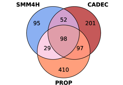
Figure 4: Venn diagram of the shared/unique PT concepts for the three datasets.

Appendix D Complete Results

Tables 3, 4 and 5 include the full results of all tested models (both Accuracy and F1 Score).

Tables 6, 7, 8, 9 and 10 report the accuracy for all the cross-dataset experiments (one table for each model).

SMM4H

		Accuracy
		in	out	overall
	CODER	32.34 ±1.22	37.47 ±2.07	32.98 ±1.24
	SAPB	42.56 ±0.50	45.98 ±3.60	43.00 ±0.77
FT	CODER	33.20 ±1.53	38.91 ±1.97	33.90 ±1.58
	SAPB	42.76 ±1.58	45.02 ±4.84	43.05 ±1.96
	PMB	50.26 ±0.95	00.00 ±0.00	44.12 ±1.24
	GPT2	72.31 ±1.55	10.02 ±2.21	64.68 ±0.98
	SCI5	34.73 ±2.05	12.63 ±3.33	32.06 ±1.84
OP	CODER	34.20 ±0.62	42.25 ±1.86	35.19 ±0.65
	SAPB	44.29 ±1.91	51.25 ±6.04	45.15 ±2.31
	PMB	51.33 ±1.15	44.25 ±2.10	50.46 ±1.18
	GPT2	41.17 ±0.52	44.48 ±4.90	41.60 ±1.05
	SCI5	40.90 ±0.80	40.56 ±6.90	40.90 ±1.48
OP+FT	CODER	34.33 ±0.80	43.24 ±1.40	35.43 ±0.83
	SAPB	45.75 ±0.66	47.76 ±7.09	46.03 ±1.36
	PMB	74.10 ±2.55	37.46 ±4.10	69.64 ±1.80
	GPT2	73.71 ±1.29	31.25 ±3.37	68.52 ±1.30
	SCI5	60.76 ±0.91	37.87 ±3.21	57.98 ±0.97

F1 Score
in	out	overall
13.52 ±0.96	23.67 ±1.42	16.34 ±1.14
16.91 ±0.57	29.93 ±3.32	20.23 ±0.20
14.12 ±1.22	24.67 ±1.16	17.14 ±1.34
16.80 ±0.78	29.58 ±4.68	20.10 ±1.17
21.43 ±1.91	00.00 ±0.00	13.68 ±1.43
11.51 ±0.49	07.09 ±1.68	10.43 ±0.48
13.77 ±0.93	05.27 ±2.61	11.83 ±0.42
14.25 ±0.81	27.30 ±1.20	17.93 ±0.83
17.96 ±1.03	35.12 ±4.84	22.27 ±1.45
25.87 ±1.21	27.95 ±0.84	27.51 ±1.41
17.50 ±0.89	24.29 ±4.18	19.63 ±1.47
17.13 ±1.05	22.70 ±2.60	18.99 ±1.37
14.40 ±0.64	28.19 ±1.02	18.18 ±0.65
18.43 ±1.17	32.04 ±5.22	21.92 ±1.66
55.59 ±3.08	22.49 ±2.73	45.62 ±2.51
52.52 ±2.61	19.59 ±2.53	42.20 ±2.68
32.25 ±2.85	23.50 ±2.83	30.08 ±1.77

Table 3: Full metrics (accuracy and F1 score) of all tested models on the SMM4H dataset.

CADEC

		Accuracy
		in	out	overall
	CODER	35.44 ±0.40	44.79 ±3.35	35.89 ±0.42
	SAPB	39.57 ±1.05	51.34 ±4.67	40.14 ±1.14
FT	CODER	39.13 ±1.54	45.96 ±2.15	39.46 ±1.45
	SAPB	48.04 ±4.03	46.48 ±4.49	47.97 ±3.70
	PMB	82.47 ±0.27	00.00 ±0.00	78.49 ±0.10
	GPT2	84.70 ±0.42	07.40 ±0.13	80.97 ±0.45
	SCI5	72.80 ±0.12	15.94 ±1.37	70.05 ±0.17
OP	CODER	41.98 ±0.65	48.06 ±3.12	42.26 ±0.65
	SAPB	69.49 ±0.37	50.53 ±1.40	68.58 ±0.37
	PMB	73.64 ±0.35	47.05 ±0.50	72.36 ±0.40
	GPT2	68.35 ±0.22	43.29 ±2.47	67.14 ±0.22
	SCI5	65.99 ±0.58	44.73 ±2.22	64.96 ±0.45
OP+FT	CODER	42.08 ±0.80	48.34 ±2.86	42.38 ±0.75
	SAPB	62.02 ±2.06	48.44 ±1.74	61.38 ±1.91
	PMB	87.18 ±0.33	23.88 ±1.79	84.12 ±0.28
	GPT2	86.08 ±0.78	23.92 ±1.09	83.08 ±0.69
	SCI5	80.96 ±0.40	37.21 ±4.32	78.85 ±0.52

F1 Score
in	out	overall
17.78 ±0.43	26.81 ±2.20	19.89 ±0.58
17.44 ±0.63	31.62 ±3.29	20.20 ±0.56
18.72 ±0.54	27.53 ±1.46	20.88 ±0.38
20.25 ±1.50	27.02 ±3.67	22.11 ±0.62
47.64 ±1.29	00.00 ±0.00	33.32 ±1.44
30.97 ±0.50	08.31 ±0.83	25.00 ±0.40
37.02 ±1.63	07.11 ±3.29	29.84 ±1.39
24.40 ±1.78	27.12 ±3.61	25.25 ±1.95
27.48 ±0.81	32.38 ±1.54	29.39 ±0.32
38.46 ±1.36	32.21 ±1.40	38.47 ±0.65
28.76 ±1.20	28.75 ±1.23	29.66 ±1.35
27.10 ±1.09	27.27 ±1.49	27.98 ±0.86
20.77 ±0.66	29.52 ±1.66	23.31 ±0.71
27.20 ±0.82	29.45 ±1.59	28.68 ±0.54
70.43 ±1.00	15.74 ±1.15	55.78 ±0.36
64.17 ±2.89	15.07 ±0.67	51.05 ±1.04
50.09 ±2.36	22.66 ±2.23	44.36 ±2.11

Table 4: Full metrics (accuracy and F1 score) of all tested models on the CADEC dataset.

PROP

		Accuracy
		in	out	overall
	CODER	12.58 ±0.44	28.44 ±3.02	14.19 ±0.71
	SAPB	20.28 ±0.59	36.54 ±3.61	21.91 ±0.81
FT	CODER	19.88 ±0.89	28.39 ±3.81	20.76 ±1.20
	SAPB	33.77 ±2.57	36.34 ±3.71	34.02 ±2.63
	PMB	60.20 ±0.34	00.00 ±0.00	54.09 ±0.76
	GPT2	65.21 ±0.73	05.75 ±1.22	59.18 ±1.12
	SCI5	45.70 ±0.77	12.71 ±1.13	42.34 ±0.61
OP	CODER	15.29 ±0.24	30.62 ±1.97	16.84 ±0.38
	SAPB	24.10 ±0.76	43.80 ±2.54	26.09 ±0.85
	PMB	30.99 ±1.00	37.92 ±1.66	31.69 ±1.04
	GPT2	24.05 ±0.77	32.89 ±2.23	24.94 ±0.86
	SCI5	24.71 ±0.78	32.71 ±4.80	25.49 ±1.12
OP+FT	CODER	19.64 ±0.25	32.88 ±2.51	20.98 ±0.28
	SAPB	39.88 ±3.20	42.68 ±3.66	40.16 ±3.23
	PMB	68.89 ±1.17	25.60 ±1.91	64.50 ±1.48
	GPT2	66.90 ±0.61	21.75 ±2.16	62.31 ±1.10
	SCI5	54.07 ±0.54	27.42 ±4.77	51.34 ±0.81

F1 Score
in	out	overall
08.02 ±0.56	16.79 ±1.30	10.79 ±0.83
10.43 ±0.33	22.50 ±2.83	13.67 ±0.83
10.18 ±0.77	15.85 ±2.01	12.23 ±0.84
12.20 ±0.77	22.41 ±2.96	15.35 ±1.14
25.56 ±0.66	00.00 ±0.00	14.66 ±0.96
17.50 ±0.50	07.90 ±0.63	13.91 ±0.31
20.80 ±1.26	07.76 ±0.49	17.31 ±1.51
09.61 ±0.66	17.79 ±0.70	12.35 ±0.51
12.71 ±0.83	27.30 ±2.13	16.67 ±0.93
20.89 ±1.88	23.60 ±1.39	22.75 ±1.66
11.36 ±0.78	19.54 ±3.04	13.38 ±1.18
10.86 ±0.66	19.73 ±1.98	13.10 ±0.85
11.38 ±0.32	19.27 ±1.27	14.22 ±0.51
16.11 ±1.88	26.86 ±2.79	19.61 ±2.09
54.19 ±2.05	16.35 ±1.59	39.66 ±2.77
49.29 ±1.26	13.41 ±1.28	35.12 ±2.52
33.36 ±1.16	17.15 ±2.70	27.89 ±2.35

Table 5: Full metrics (accuracy and F1 score) of all tested models on the PROP dataset.

CODER FT

		Test (in)
		CADEC	SMM4H	PROP
Train	CADEC	39.13	35.80	31.84
	SMM4H	37.78	33.20	40.44
	PROP	37.83	35.08	19.88

Test (out)
CADEC	SMM4H	PROP
45.96	35.79	08.79
31.87	38.91	09.39
35.73	32.56	28.39

Test (overall)
CADEC	SMM4H	PROP
39.46	35.82	15.25
36.00	33.90	14.25
37.39	33.85	20.76

CODER OP+FT

		Test (in)
		CADEC	SMM4H	PROP
Train	CADEC	42.08	35.12	33.56
	SMM4H	44.90	34.33	43.95
	PROP	44.25	38.62	19.64

Test (out)
CADEC	SMM4H	PROP
48.34	35.63	11.34
36.72	43.24	12.81
37.77	32.21	32.88

Test (overall)
CADEC	SMM4H	PROP
42.38	35.25	17.59
42.42	35.43	17.69
42.85	35.49	20.98

Table 6: Cross-dataset accuracy for CODER FT and CODER OP+FT on the three datasets.

SapBERT FT

		Test (in)
		CADEC	SMM4H	PROP
Train	CADEC	42.69	35.09	30.80
	SMM4H	39.14	39.58	39.92
	PROP	32.21	31.07	26.69

Test (out)
CADEC	SMM4H	PROP
34.47	35.32	8.73
23.79	32.42	10.02
29.77	34.97	25.81

Test (overall)
CADEC	SMM4H	PROP
42.30	35.12	14.94
34.53	38.69	14.71
31.71	32.98	26.60

SapBERT OP+FT

		Test (in)
		CADEC	SMM4H	PROP
Train	CADEC	63.96	45.93	49.29
	SMM4H	70.71	46.28	62.73
	PROP	68.69	49.77	41.33

Test (out)
CADEC	SMM4H	PROP
47.76	34.72	14.63
61.31	48.43	17.84
48.09	28.82	39.81

Test (overall)
CADEC	SMM4H	PROP
63.19	42.65	24.39
67.89	46.54	24.90
64.24	39.45	41.17

Table 7: Cross-dataset accuracy for SapBERT FT and SapBERT OP+FT on the three datasets.

PMB FT

		Test (in)
		CADEC	SMM4H	PROP
Train	CADEC	82.47	54.00	51.74
	SMM4H	38.82	50.26	31.43
	PROP	47.76	39.83	60.20

Test (out)
CADEC	SMM4H	PROP
00.00	00.00	00.00
00.00	00.00	00.00
00.00	00.00	00.00

Test (overall)
CADEC	SMM4H	PROP
78.49	38.00	14.55
27.16	44.12	04.93
37.48	20.22	54.09

PMB OP+FT

		Test (in)
		CADEC	SMM4H	PROP
Train	CADEC	87.18	61.05	64.95
	SMM4H	79.84	74.10	79.24
	PROP	75.33	63.33	68.89

Test (out)
CADEC	SMM4H	PROP
23.88	18.76	11.64
53.14	37.46	17.35
39.84	23.86	25.60

Test (overall)
CADEC	SMM4H	PROP
84.12	48.54	26.64
71.82	69.64	27.07
67.72	43.88	64.50

Table 8: Cross-dataset accuracy for PMB FT and PMB OP+FT on the three datasets.

GPT-2 FT

		Test (in)
		CADEC	SMM4H	PROP
Train	CADEC	84.70	60.86	60.52
	SMM4H	65.73	72.31	69.88
	PROP	56.68	52.43	65.21

Test (out)
CADEC	SMM4H	PROP
07.40	03.78	01.51
06.54	10.02	01.84
07.41	03.45	05.75

Test (overall)
CADEC	SMM4H	PROP
80.97	43.99	18.10
47.94	64.68	12.52
46.08	28.31	59.18

GPT-2 OP+FT

		Test (in)
		CADEC	SMM4H	PROP
Train	CADEC	86.08	62.50	62.56
	SMM4H	78.23	73.71	77.98
	PROP	72.75	58.96	66.90

Test (out)
CADEC	SMM4H	PROP
23.92	34.21	08.90
26.72	31.25	11.02
27.65	18.72	21.75

Test (overall)
CADEC	SMM4H	PROP
83.08	54.06	24.00
62.74	68.52	21.54
63.09	39.15	62.31

Table 9: Cross-dataset accuracy for GPT-2 FT and GPT-2 OP+FT on the three datasets.

Sci5 FT

		Test (in)
		CADEC	SMM4H	PROP
Train	CADEC	72.80	44.44	46.20
	SMM4H	35.28	34.73	44.05
	PROP	29.23	28.44	45.70

Test (out)
CADEC	SMM4H	PROP
15.94	06.86	03.07
10.42	12.63	03.30
15.44	11.14	12.71

Test (overall)
CADEC	SMM4H	PROP
70.05	33.33	15.19
27.81	32.06	09.71
26.24	19.93	42.34

Sci5 OP+FT

		Test (in)
		CADEC	SMM4H	PROP
Train	CADEC	80.96	56.07	60.35
	SMM4H	71.96	60.76	72.82
	PROP	63.63	47.74	54.07

Test (out)
CADEC	SMM4H	PROP
37.21	36.86	13.95
52.17	37.87	17.19
40.12	26.95	27.42

Test (overall)
CADEC	SMM4H	PROP
78.85	50.34	27.02
66.02	57.98	25.92
58.52	37.45	51.34

Table 10: Cross-dataset accuracy for Sci5 FT and Sci5 OP+FT on the three datasets.

References

- Bodenreider (2004) Olivier Bodenreider. 2004. The Unified Medical Language System (UMLS): Integrating Biomedical Terminology. Nucleic Acids Research, 32:D267–70.
- Brown et al. (1999) Elliot G Brown, Louise Wood, and Sue Wood. 1999. The Medical Dictionary for Regulatory Activities (MedDRA). Drug Safety, 20(2):109–117.
- Devlin et al. (2019) Jacob Devlin, Ming-Wei Chang, Kenton Lee, and Kristina Toutanova. 2019. BERT: Pre-training of Deep Bidirectional Transformers for Language Understanding. In Proceedings of NAACL.
- Gonzalez-Hernandez et al. (2020) Graciela Gonzalez-Hernandez, Ari Z. Klein, Ivan Flores, Davy Weissenbacher, Arjun Magge, Karen O’Connor, Abeed Sarker, Anne-Lyse Minard, Elena Tutubalina, Zulfat Miftahutdinov, and Ilseyar Alimova. 2020. Proceedings of the COLING Social Media Mining for Health Applications Workshop & Shared Task.
- Gu et al. (2020) Yu Gu, Robert Tinn, Hao Cheng, Michael Lucas, Naoto Usuyama, Xiaodong Liu, Tristan Naumann, Jianfeng Gao, and Hoifung Poon. 2020. Domain-Specific Language Model Pretraining for Biomedical Natural Language Processing. arXiv preprint arXiv:2007.15779.
- Halder et al. (2020) Kishaloy Halder, Alan Akbik, Josip Krapac, and Roland Vollgraf. 2020. Task-aware Representation of Sentences for Generic Text Classification. In Proceedings of COLING.
- Karimi et al. (2015) Sarvnaz Karimi, Alejandro Metke-Jimenez, Madonna Kemp, and Chenchen Wang. 2015. Cadec: A Corpus of Adverse Drug Event Annotations. Journal of Biomedical Informatics, 55:73–81.
- Leaman et al. (2013) Robert Leaman, Rezarta Islamaj Doğan, and Zhiyong Lu. 2013. DNorm: Disease Name Normalization with Pairwise Learning to Rank. Bioinformatics, 29(22):2909–2917.
- Li et al. (2017) Haodi Li, Qingcai Chen, Buzhou Tang, Xiaolong Wang, Hua Xu, Baohua Wang, and Dong Huang. 2017. CNN-based Ranking for Biomedical Entity Normalization. BMC Bioinformatics, 18(11):79–86.
- Limsopatham and Collier (2016) Nut Limsopatham and Nigel Collier. 2016. Normalising Medical Concepts in Social Media Texts by Learning Semantic Representation. In Proceedings of ACL.
- Liu et al. (2021) Fangyu Liu, Ehsan Shareghi, Zaiqiao Meng, Marco Basaldella, and Nigel Collier. 2021. Self-Alignment Pretraining for Biomedical Entity Representations. pages 4228–4238.
- Niu et al. (2019) Jinghao Niu, Yehui Yang, Siheng Zhang, Zhengya Sun, and Wensheng Zhang. 2019. Multi-task Character-level Attentional Networks for Medical Concept Normalization. Neural Processing Letters, 49(3):1239–1256.
- Phan et al. (2021) Long N. Phan, James T. Anibal, Hieu Tran, Shaurya Chanana, Erol Bahadroglu, Alec Peltekian, and Grégoire Altan-Bonnet. 2021. SciFive: A Text-to-text Transformer Model for Biomedical Literature. arXiv preprint arXiv:2106.03598.
- Portelli et al. (2021) Beatrice Portelli, Edoardo Lenzi, Emmanuele Chersoni, Giuseppe Serra, and Enrico Santus. 2021. BERT Prescriptions to Avoid Unwanted Headaches: A Comparison of Transformer Architectures for Adverse Drug Event Detection. In Proceedings of EACL.
- Radford et al. (2019) Alec Radford, Jeff Wu, Rewon Child, David Luan, Dario Amodei, and Ilya Sutskever. 2019. Language Models are Unsupervised Multitask Learners. OpenAI Blog.
- Scaboro et al. (2021) Simone Scaboro, Beatrice Portelli, Emmanuele Chersoni, Enrico Santus, and Giuseppe Serra. 2021. NADE: A Benchmark for Robust Adverse Drug Events Extraction in Face of Negations. In Proceedings of the EMNLP Workshop on Noisy User-Generated Text.
- Scaboro et al. (2022) Simone Scaboro, Beatrice Portelli, Emmanuele Chersoni, Enrico Santus, and Giuseppe Serra. 2022. Increasing Adverse Drug Events Extraction Robustness on Social Media: Case Study on Negation and Speculation. arXiv preprint arXiv:2209.02812.
- Sung et al. (2020) Mujeen Sung, Hwisang Jeon, Jinhyuk Lee, and Jaewoo Kang. 2020. Biomedical Entity Representations with Synonym Marginalization. In Proceedings of ACL.
- Tutubalina et al. (2018) Elena Tutubalina, Zulfat Miftahutdinov, Sergey Nikolenko, and Valentin Malykh. 2018. Medical Concept Normalization in Social Media Posts with Recurrent Neural Networks. Journal of Biomedical Informatics, 84:93–102.
- Yuan et al. (2022) Zheng Yuan, Zhengyun Zhao, Haixia Sun, Jiao Li, Fei Wang, and Sheng Yu. 2022. CODER: Knowledge-infused Cross-lingual Medical Term Embedding for Term Normalization. Journal of Biomedical Informatics, 126:103983.
- Zhang et al. (2021) Sheng Zhang, Hao Cheng, Shikhar Vashishth, Cliff Wong, Jinfeng Xiao, Xiaodong Liu, Tristan Naumann, Jianfeng Gao, and Hoifung Poon. 2021. Knowledge-Rich Self-Supervised Entity Linking. CoRR, abs/2112.07887.
- Ziletti et al. (2022) Angelo Ziletti, Alan Akbik, Christoph Berns, Thomas Herold, Marion Legler, and Martina Viell. 2022. Medical coding with biomedical transformer ensembles and zero/few-shot learning. In Proceedings of the 2022 Conference of the North American Chapter of the Association for Computational Linguistics: Human Language Technologies: Industry Track, pages 176–187, Hybrid: Seattle, Washington + Online. Association for Computational Linguistics.