Pauli-Term-Induced Fixed Points in $d$-dimensional QED

Abstract

We explore the fixed-point structure of QED-like theories upon the inclusion of a Pauli spin-field coupling. We concentrate on the fate of UV-stable fixed points recently discovered in $d=4$ spacetime dimensions upon generalizations to lower as well as higher dimensions for an arbitrary number of fermion flavors $N_{\text{f}}$. As an overall trend, we observe that going away from $d=4$ dimensions and increasing the flavor number tends to destabilize the non-Gaussian fixed points discovered in four spacetime dimensions. A notable exception is a non-Gaussian fixed point at finite Pauli spin-field coupling but vanishing gauge coupling, which also remains stable down to $d=3$ dimensions and for small flavor numbers. This includes also the range of degrees of freedom used in effective theories of layered condensed-matter systems. As an application, we construct renormalization group trajectories that emanate from the non-Gaussian fixed point and approach a long-range regime in the conventional QED₃ universality class that is governed by the interacting (quasi) fixed point in the gauge coupling.

I Introduction

The Pauli term, denoting the coupling between the electron spin and the electromagnetic field, plays an interesting role in quantum electrodynamics (QED): it undergoes finite renormalization [1] while receiving contributions from all scales [2, 3]; in the effective action, it parameterizes the famous anomalous magnetic moment of the electron [4, 5] which has been measured and computed to an extraordinary precision [6, 7, 8]; and from a Wilsonian viewpoint, it corresponds to a perturbatively nonrenormalizable dimension-5 operator and thus has the least possible finite distance to the set of renormalizable operators in QED theory space.

Specifically the last property makes the Pauli term a candidate for a relevant interaction in a coupling regime where nonperturbative interactions set in. In fact, a recent study [9] provides evidence that the observed long-range properties of (pure) QED can be extended to high-energy scales along renormalization group (RG) trajectories that exhibit a sizable Pauli-term contribution. Remarkably, a systematic next-to-leading order expansion of the effective action features nonperturbative ultraviolet (UV) stable fixed points that give rise to a UV-complete version of QED within an asymptotic-safety scenario [10, 11]. The possibility that a sizable Pauli term could be sufficient for QED to evade the infamous Landau-pole problem [12] had already been suggested in [13] on the basis of an effective-field-theory study.

It is important to note that the Pauli-term-induced UV-completion of QED also evades the conclusion of QED triviality from previous analyses of QED in the strong-coupling regime on the lattice [14] as well as using the functional RG [15]. The reason is that the Pauli term goes beyond the chirally invariant subspace of massless QED; moreover, one of the non-Gaussian fixed points occurs at vanishing gauge coupling. QED triviality observed in [14, 15] relies on the observation of chiral symmetry breaking induced by a strong gauge coupling which prohibits the connection of a strongly coupled high-energy regime to the observed phase with a light electron. As a caveat, we should mention that the potential of the Pauli term to generate a heavy electron mass has not yet been explored.

The findings of [9] serve as a strong inspiration to study the Pauli term and the fate of the corresponding nonperturbative fixed points also in dimensions larger and smaller than $d=4$. Specifically $d=3$ is a relevant case, since QED₃ serves as an effective theory for the long-range excitations of various layered condensed-matter systems [16, 17, 18, 19, 20, 21, 22, 23, 24] including graphene and cuprate superconductors. In this context, also the dependence of the renormalization structure of the theory on the number of fermion flavors $N_{\text{f}}$ is of substantial interest: the question as to whether the long-range properties of QED₃ depend on the flavor number and whether quantum phase transitions as a function of $N_{\text{f}}$ exist has a long tradition in the literature [25, 26, 27, 28, 29, 30, 31, 32, 33, 34, 35, 36, 37, 38, 39, 40, 41, 42, 43, 44, 45, 46, 47, 48, 49, 50, 51, 52, 53, 54, 55, 56, 57, 58, 59, 60, 61].

At the same time, it is interesting to explore the features of the system towards higher dimensions: whereas perturbative renormalization clearly favors four dimensional spacetime as a setting where interacting field theories of scalar and fermionic matter with gauge interactions can exist over a wide range of scales, the possibility of nonperturbative fixed points appears to loosen this connection between the existence of interacting quantum field theories and the observed dimensionality of spacetime. Still, various studies find that evidence for nonperturbative UV completions appears to become less robust beyond $d=4$ dimensions [62, 63, 64, 65, 66, 67, 68, 69, 70, 71, 72].

We start by introducing the model in general dimensions in Sect. II. Section III briefly reviews the results derived in [9] as a reference point for our investigations of lower (Sect. IV) and higher (Sect. V) dimensional spacetimes. Our conclusions are given in Sect. VI.

II QED_d with a Pauli term

We investigate QED_d, i.e. QED in $d$ spacetime dimensions, with $N_{\text{f}}$ Dirac flavors $\psi^{a}$ interacting with an electromagnetic field $A_{\mu}$. In addition to the conventional gauge interaction, we include a Pauli spin-field coupling already on the level of the bare action. Throughout this work, we use Euclidean conventions in which the bare action satisfying Osterwalder-Schrader positivity reads

$$S\!=\!\int_{x}\frac{1}{4}F_{\mu\nu}F^{\mu\nu}+\bar{\psi}^{a}i\not{D}[A]\psi^{a}-i\bar{m}\bar{\psi}^{a}\psi^{a}+i\bar{\kappa}\bar{\psi}^{a}\sigma_{\mu\nu}F^{\mu\nu}\psi^{a},$$ (1)

Here the covariant derivative is defined as $D_{\mu}[A]=\partial_{\mu}-i\bar{e}A_{\mu}$. All mass and coupling parameters are understood to denote bare quantities. While the kinetic term is chirally invariant, the mass term $\sim\bar{m}$ and the Pauli term $\sim\bar{\kappa}$ break chiral symmetry explicitly.

In this work, we study the renormalization flow of the couplings and the mass, also allowing for wave function renormalizations $Z_{\psi,A}$ that renormalize the fields of a Wilsonian-type action of the form of Eq. (1) multiplicatively, $\psi\to\sqrt{Z_{\psi}}\psi$, $A\to\sqrt{Z_{A}}A$. This allows us to define the corresponding renormalized couplings. For our present goal of searching for fixed points, where the theory becomes (quantum) scale invariant, it is useful to introduce dimensionless renormalized quantities:

$$e=\frac{k^{\frac{d}{2}-2}\bar{e}}{Z_{\psi}\sqrt{Z_{A}}},\quad m=\frac{\bar{m}}{Z_{\psi}k},\quad\kappa=\frac{k^{\frac{d}{2}-1}\bar{\kappa}}{Z_{\psi}\sqrt{Z_{A}}},$$ (2)

where $k$ denotes an RG scale that is used to parameterize RG trajectories in the space of couplings. The exponents of $k$ reflect the canonical scaling of the corresponding operators. For instance, the gauge coupling $e$ is power-counting marginal in $d=4$, relevant in $d<4$ and irrelevant in higher dimensions. The mass term is a relevant operator in any dimension, whereas the Pauli term is power-counting irrelevant in all dimensions $d>2$. Note, however, that the Pauli term, being a dimension-5 operator in $d=4$, has the smallest possible distance to marginality in an operator expansion of the action. In addition, it is a leading term in a derivative expansion, in which the only other dimension-5 term $\sim\bar{\psi}\not{D}\not{D}\psi$ is subleading.

Even though the canonical scaling fully governs RG (ir-)relevance in the perturbative regime, where corrections to scaling can only be logarithmic according to Weinberg’s theorem [73], nonperturbative phenomena can be characterized by large anomalous dimensions and thus strongly affect canonical scaling. In both $d=4$ and $d=3$, the nonperturbative phenomenon of chiral symmetry breaking is a prime example for this: at large coupling, the anomalous dimensions of the fermionic self-interaction operators of the type $\mathcal{O}_{\psi^{4}}\sim(\bar{\psi}\psi)^{2}$ can result in RG relevance and induce a chiral condensate. This can occur in both $d=4$ [74, 75, 76], where $\mathcal{O}_{\psi^{4}}$ is a dimension-6 operator, as well as in $d=3$ [36, 35, 77, 44] where it is a dimension-4 operator. These observations put an even stronger emphasis on the question of a possible RG relevance of the Pauli term in the nonperturbative regime, as it is closest to marginality.

We approach the answer to this question by studying the phase diagram of QED_d. More specifically, we use the Wetterich equation [78, 79, 80, 81], a functional RG flow equation, and determine the $\beta$ functions of the couplings $e$, $m$, and $\kappa$. Using $t=\ln k$ as a flow parameter, the $\beta$ functions can be written as

$$\partial_{t}e = \beta_{e}=e\left(\frac{d}{2}-2+\eta_{\psi}+\frac{\eta_{A}}{2}\right)+\Delta\beta_{e},$$ (3)

$$\partial_{t}m = \beta_{m}=-m\left(1-\eta_{\psi}\right)+\Delta\beta_{m},$$ (4)

$$\partial_{t}\kappa = \beta_{\kappa}=\kappa\left(\frac{d}{2}-1+\eta_{\psi}+\frac{\eta_{A}}{2}\!\right)+\Delta\beta_{\kappa},$$ (5)

where $\eta_{\psi,A}$ denote the anomalous dimensions obtained from

$$\eta_{\psi}=-\partial_{t}\ln Z_{\psi},\quad\eta_{A}=-\partial_{t}\ln Z_{A}.$$ (6)

In Eqs. (3)-(5), we highlighted the dimensional scaling terms explicitly, which reflect the canonical scaling exponents already displayed in Eq. (2) together with the anomalous dimensions $\eta_{\psi,A}$. The last terms $\Delta\beta_{e,m,\kappa}$ abbreviate the quantum (loop) contributions. Their explicit forms have been computed in [9] and are summarized in Appendix A to next-to-leading order in a systematic expansion scheme of the Wetterich equation. Structurally, these fluctuation contributions depend on

$$\Delta\beta=\Delta\beta(e,m,\kappa;\eta_{\psi},\eta_{A}|d,d_{\gamma}N_{\text{f}}),$$ (7)

where the anomalous dimensions satisfy algebraic equations also listed in App. A and can be expressed as functions of the couplings as well. In addition to a parametric dependence on the dimension $d$, the $\beta$ functions also depend on the product $d_{\gamma}N_{\text{f}}$ counting the number of spinor degrees of freedom: in addition to the flavor number $N_{\text{f}}$, $d_{\gamma}$ denotes the dimensionality of the representation of the Dirac algebra. The irreducible representations satisfy $d_{\gamma}=2^{\lfloor d/2\rfloor}$ which is used below unless specified otherwise.

Rather generally, the $\beta$ functions (3)-(5) are not universal, but also depend on the details of the regularization. Even perturbatively, only the one- and two-loop coefficient of the marginal coupling $e$ in $d=4$ are universal in a mass-independent scheme. Since we include the running of the mass and pay attention to threshold effects, we work with a standard mass-scale-dependent functional RG scheme. Nevertheless, the existence of fixed points of the RG, where all $\beta$ functions vanish, is a universal statement. Summarizing the couplings and the $beta$ functions in vector-like quantities, $\mathbf{g}=(e,\kappa,m)$, $\bm{\beta}=(\beta_{e},\beta_{\kappa},\beta_{m})$, a fixed point $\mathbf{g}^{\ast}$ satisfies $\bm{\beta}(\mathbf{g}=\mathbf{g}^{\ast})=0$. In addition, the critical exponents $\theta_{I}$ at a fixed point are also universal. Linearizing the $\beta$ functions near a fixed point, the flow is governed by the stability matrix $\mathbf{B}$, the eigenvalues of which determine the critical exponents,

$$\mathbf{B}_{ij}=\frac{\partial\beta_{g_{i}}}{\partial g_{j}}\Big{|}_{\mathbf{g}=\mathbf{g}^{\ast}},\quad\theta_{I}=-\text{eig}(\mathbf{B}).$$ (8)

Since we work in an approximation scheme, our results for the universal quantities listed in the following also exhibit only approximate universality and thus depend on the scheme to some extent. For concrete computations, we use the partially linear regularization scheme which is known to be optimized for fast convergence to universal results in a class of approximations also used here [82, 83].

Positive (negative) critical exponents $\theta_{i}>0$ ($\theta_{i}<0$) are associated with relevant (irrelevant) directions. The eigendirections associated with the positive exponents span the UV critical surface of trajectories emanating from the fixed point. The dimensionality of this surface, and thus the number of positive exponents, is equal to the number of physical parameters to be fixed in order to render the long-range behavior of the theory fully computable. (Eigenvalues $\theta_{I}=0$ denote marginal directions; here, higher orders beyond the linearized flow determine relevance or irrelevance. For instance, the QED₄ gauge coupling $e$ is marginally irrelevant.)

In addition to gauge symmetry as a local redundancy, the action has a global U($N_{\text{f}}$) flavor symmetry, whereas an extended U$(N_{\text{f}})_{\text{L}}\times$U$(N_{\text{f}})_{\text{R}}$ chiral symmetry is present only in the absence of the mass and the Pauli term, $m=0$ and $\kappa=0$. In the general case, the action is also invariant under a discrete axial rotation of the spinors by an angle of $\pi/2$ and a simultaneous sign flip of $\kappa$ and $m$, as well as under charge conjugation and a simultaneous sign flip of $e$ and $\kappa$. These latter $\mathbb{Z}_{2}$ symmetries are also visible on the level of the flow equations which remain invariant under $(e,\kappa,m)\to(e,-\kappa,-m)$ and $(e,\kappa,m)\to(-e,-\kappa,m)$ as well as combinations thereof. Correspondingly, fixed points can exist in these sign-flip multiplicities, but, of course, describe one and the same universality class.

In the following, results for fixed-point searches in various dimensions and for various fermion degrees of freedom (flavor number, spinor representation) are presented. As fixed points at finite couplings are an inherently nonperturbative phenomenon, it is important to discuss consistency criteria in the absence of a generically small control parameter. Our systematic approximation scheme represents a combined expansion in operator dimension and in derivatives. In this sense, the inclusion of wave function renormalizations $Z_{\psi,A}$ already represents a next-to-leading order contribution. As a quantitative control, we can compare to the leading-order result which is obtained by ignoring wave-function-renormalization effects in loop terms. In practice, this corresponds to setting $\eta_{\psi,A}=0$ inside the loop terms (technically, inside the threshold functions, see App. A), but retaining them in the scaling terms displayed in Eqs. (3)-(5).

We list results only for fixed points where the transition from leading- to next-to-leading-order results are quantitatively controlled. This control is implemented by demanding that the anomalous dimensions remain sufficiently small, $|\eta_{\psi,A}|\lesssim\mathcal{O}(1)$. From a technical viewpoint, the flow equations (3)-(5) feature rational functions of high order in the couplings on the right-hand sides. Generically, they exhibit a large number of fixed-points, most of which do not satisfy our quality criteria and are thus considered as artifacts of our approximation. Only a small number fulfills the consistency conditions in a remarkably stable manner. These are the ones presented in the following sections.

III Pauli-term fixed points in $d=4$

As a reference point, we start by reviewing the phase diagram of QED₄ with a Pauli term for $N_{\text{f}}=1$ as has been found in the literature [9]. Generalizations to different dimensions and different flavor numbers can be well understood by analyzing the similarities and differences to this reference case.

In addition to the Gaussian fixed point $\mathcal{A}$ characterized by vanishing couplings, we find two interacting fixed points that satisfy all our consistency criteria, cf. Tab.1. Both these fixed points $\mathcal{B}$ and $\mathcal{C}$ occur at finite Pauli $\kappa$ but vanishing gauge coupling. Fixed point $\mathcal{B}$ also occurs at finite mass parameter $m$ and has full $\mathbb{Z}_{2}\times\mathbb{Z}_{2}$-fold multiplicity, whereas for fixed point $\mathcal{C}$ only the charge conjugation multiplicity is pertinent.

	$e$	$\kappa$	$m$	multiplicity	$n_{\mathrm{phys}}$	$\theta_{\mathrm{max}}$	$\eta_{\psi}$	$\eta_{\mathrm{A}}$
$\mathcal{A:}$	$0$	$0$	$0$	$-$	$1$	$1.00$	$0.00$	$0.00$
$\mathcal{B:}$	$0$	$5.09$	$0.328$	$\mathbb{Z}_{2}\times\mathbb{Z}_{2}$	$2$	$3.10$	$-1.38$	$0.53$
$\mathcal{C:}$	$0$	$3.82$	$0$	$\mathbb{Z}_{2}$	$3$	$2.25$	$-1.00$	$0.00$

Table 1: Fixed points of $d=4$ dimensional QED.

At the Gaussian fixed point $\mathcal{A}$, only the mass is a relevant direction. At fixed point $\mathcal{B}$, the direction towards finite gauge coupling also represents a relevant direction. Fixed point $\mathcal{C}$ features 3 relevant directions, implying that all couplings in the action correspond to physical parameters that define the long-range behavior of the system. The flow towards the long-range IR is visualized in the phase diagram of the $(\kappa,m)$ plane at $e=0$ in Fig. 1. Note that the rapid flow near the $m$ axis towards large values of $m$ reflects the fact that $m$ denotes a dimensionless mass parameter increasing as $m\sim 1/k$ for $k\to 0$ if the physical mass approaches a finite value.

Figure 1: Phase diagram for $d=4$, $N_{\text{f}}=1$ in the $(\kappa,m)$ plane at vanishing $e=0$ exhibiting the Gaussian fixed point $\mathcal{A}$, and the non-Gaussian fixed points $\mathcal{B}$ and $\mathcal{C}$ (a $\mathbb{Z}_{2}$ reflection of $\mathcal{B}$ is also visible). Arrows denote the renormalization group flow towards the IR. The massive phase where the dimensionless mass $m$ scales as $m\sim 1/k$ to large values is accessible from all fixed points.

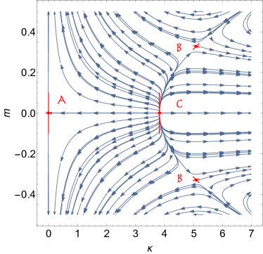
As discussed in [9], UV-complete trajectories that agree with the observed long-range behavior of pure QED₄ can be constructed with fixed point $\mathcal{C}$ as a UV fixed point. Even though UV-complete trajectories emanating from $\mathcal{B}$, of course, also exist, their long-range behavior is characterized by very large values of the anomalous magnetic moment of the electron, incompatible with observations.

Beyond arguments of physical compatibility (ultimately, pure QED is only a part of the electroweak sector), a second glance at the non-Gaussian fixed points further reveals more subtle differences: at fixed point $\mathcal{C}$, the fermion anomalous dimension is exactly $\eta_{\psi}=-1$ which is the value needed to render the Pauli coupling power-counting marginal. The fermionic scaling dimension at the fixed point becomes equivalent to that of a scalar field for this value. In order to quantify how nonperturbative the system is at the fixed points, let us introduce the quantity

$$\alpha_{\kappa}=\frac{\kappa^{2}}{4\pi},$$ (9)

in analogy to the fine-structure constant $\alpha=\frac{e^{2}}{4\pi}$. At the fixed point $\mathcal{C}$, we observe that $\alpha_{\kappa}^{\ast}\simeq 1.16$, whereas $\alpha_{\kappa}^{\ast}\simeq 2.06$ at fixed point $\mathcal{B}$. This, together with the fact that the anomalous dimensions are larger, indicates that fixed point $\mathcal{B}$ is in a significantly deeper nonperturbative region.

Let us now go beyond the literature results of [9] and study the flavor number $N_{\text{f}}$ dependence of the phase diagram for the irreducible representation $d_{\gamma}=4$. Since we have $e=0=m$ at the fixed point $\mathcal{C}$, the flow equation for the remaining coupling $\kappa$ simplifies considerably, yielding

$$\partial_{t}\kappa|_{e,m=0}=(1+\eta_{\psi})\kappa,\quad\eta_{\psi}=-\frac{3}{5\pi^{2}}\frac{\kappa^{2}}{1-\frac{3}{40\pi^{2}}\kappa^{2}}.$$ (10)

We observe that $\eta_{\psi}=-1$ is a requirement for the existence of a fixed-point at the present level of approximation which is indeed satisfied for $\mathcal{C}$. Furthermore, the flow and thus also its fixed points are completely independent of $N_{\text{f}}$. The same statement also holds for the stability matrix $\mathbf{B}$ at the fixed point and thus also for the critical exponents. We conclude that the results for fixed point $\mathcal{C}$ in Tab. 1 persist for any value of $N_{\text{f}}$.

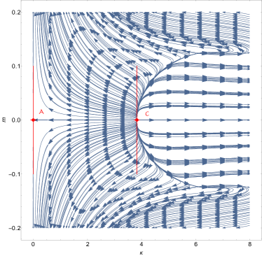
This is different for fixed point $\mathcal{B}$ where both fixed point position and critical exponents do depend on $N_{\text{f}}$. We observe that $\kappa^{\ast}$ at the fixed point increases with $N_{\text{f}}$ whereas $m^{\ast}$ decreases. At a critical value of the flavor number $N_{\text{f}}\simeq 18.50$, fixed point $\mathcal{B}$ collides with another fixed point and then disappears into the complex plane. This other fixed point comes from even larger values of the coupling and belongs to those that do not satisfy our consistency conditions at $N_{\text{f}}=1$. In fact, near the collision, fixed point $\mathcal{B}$ no longer satisfies our consistency conditions. For instance, at $N_{\text{f}}=18$, we have $\eta_{\psi}\simeq-2.65$, $\eta_{A}=3.24$, and $\kappa^{\ast}\simeq 6.13$, implying $\alpha_{\kappa}\simeq 3$. A phase diagram for $N_{\text{f}}=19$ where $\mathcal{B}$ has disappeared is shown in Fig. 2.

Figure 2: Phase diagram for $d=4$, $N_{\text{f}}=19$ in the $(\kappa,m)$ plane at vanishing $e=0$. In comparison to $N_{\text{f}}=1$, the fixed point $\mathcal{B}$ has disappeared as a consequence of a fixed point collision, whereas the Gaussian fixed point $\mathcal{A}$ and the non-Gaussian fixed point $\mathcal{C}$ persist for all values of $N_{\text{f}}$.

As a summary of the $d=4$ dimensional theory, we find that fixed point $\mathcal{C}$ exists for all values of $N_{\text{f}}$, remains quantitatively stable and supports UV-complete trajectories that can be matched to the physical long-range observables. By contrast, fixed point $\mathcal{B}$ becomes less consistent with increasing $N_{\text{f}}$ and disappears for large $N_{\text{f}}$ in a fixed-point collision. Since this collision occurs in a regime which is not well controlled in our approximation, we anticipate that the critical flavor number estimated here as $N_{\text{f}}\simeq 18.50$ can undergo large corrections upon improvements of the approximation.

IV Pauli-term fixed points in lower dimensions

In spacetime dimensions lower than four, $d<4$, the RG flow of the couplings exhibits both qualitative as well as quantitative changes. Quantitatively, we observe in Eqs. (A)-(18) that a sizable number of terms have a prefactor $(d-4)$ and thus contribute only away from $d=4$.

Qualitatively, a major change occurs, since the scaling term of the gauge coupling flow Eq. (3) now contributes to linear order in $e$, i.e., $\partial_{t}e=-\frac{1}{2}e+\mathcal{O}(e^{3},\dots)$. Provided that the loop terms of higher order are sufficiently positive, a new fixed point $\mathcal{D}$ emerges on the positive $e$ axis (with a corresponding $\mathbb{Z}_{2}$ reflection at negative values of $e$). The occurrence of this fixed point $\mathcal{D}$ is well known in the literature [84, 85, 25]. It is infrared (IR) attractive in the coupling flow in contrast to the Gaussian fixed point $\mathcal{A}$ at which the gauge coupling $e$ now parameterizes a relevant IR-repulsive interaction.

The fixed-point value $e^{\ast}$ at $\mathcal{D}$ is decisive for the long-range behavior of the lower-dimensional QED. If $e^{\ast}$ is sufficiently weak, chiral symmetry can persist: along a trajectory emanating from the Gaussian fixed point $\mathcal{A}$, the system remains massless and the theory can be IR conformal. For such trajectories, $e^{\ast}$ at $\mathcal{D}$ represents the maximum long-range coupling strength of the theory.

If this maximum coupling is sufficiently large, it has the potential to trigger chiral symmetry breaking and the formation of chiral condensates. From an RG picture, symmetry breaking can proceed via induced fermionic self-interactions becomes relevant [36, 35, 44], rendering fixed point $\mathcal{D}$ unstable through a fixed-point collision; in this case, $\mathcal{D}$ represents a quasi fixed point that exists only for a finite range of the RG flow and disappears in the deep IR. Whether this occurs or not in the physically relevant case $d=3$, and for which range of $N_{\text{f}}$, has been a major research thread in the past decades [25, 26, 27, 28, 29, 30, 31, 32, 33, 34, 35, 36, 37, 38, 39, 40, 41, 42, 43, 44, 45, 46, 47, 48, 49, 50, 51, 52, 53, 54, 55, 56, 57, 58, 59, 60, 61] with different methods yielding different answers.

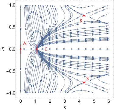
While the present work has nothing to add to the question of chiral symmetry breaking of the system at or near fixed point $\mathcal{D}$, let us now study how the Pauli coupling complements the phase diagram away from the chirally symmetric subspace. In fact, we observe the existence of the Pauli-coupling fixed point $\mathcal{C}$ for all lower dimensions in between $2<d<4$ with qualitative properties similar to $d=4$ for sufficiently small flavor numbers. For the relevant case of $d=3$ and $N_{\text{f}}=1$ irreducible Dirac flavors with $d_{\gamma}=2$, both non-Gaussian fixed points can be seen in the $(e,\kappa)$ plane at $m=0$ in Fig. 3. This phase diagram illustrates that fixed point $\mathcal{D}$ remains IR attractive also in the direction of the chiral symmetry breaking Pauli coupling; by contrast, a mass-type perturbation remains relevant. We also observe that fixed point $\mathcal{C}$ is fully repulsive. Quantitatively, it is interesting to see that the fixed-point value of the Pauli coupling at $\mathcal{C}$ decreases with decreasing dimension; e.g., we have $\alpha_{\kappa}\simeq 0.1$ at $d=3$.

Figure 3: Phase diagram for $d=3$, $N_{\text{f}}=1$ in the $(e,\kappa)$ plane at vanishing $m=0$ for the irreducible representation $d_{\gamma}=2$. The IR-attractive fixed point $\mathcal{D}$ is characteristic for lower-dimensional QED. It can characterize a chirally invariant long-range conformal phase or–if sufficiently strongly coupled–trigger dynamical chiral symmetry breaking. This fixed point also remains IR attractive in the direction of the Pauli coupling.

Figure 4: Phase diagram for $d=3$, $N_{\text{f}}=1$ in the $(\kappa,m)$ plane at vanishing $e=0$ for the irreducible representation $d_{\gamma}=2$. In comparison to Fig. 1 in $d=4$, the fixed point $\mathcal{C}$ is more weakly coupled.

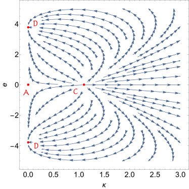
Quantitative results for the fixed points for $d=3$ and $N_{\text{f}}=1$ irreducible flavors are listed in Tab. 2. In addition, the non-Gaussian fixed point $\mathcal{B}$ is present at smaller values of $\kappa^{\ast}$ but larger mass parameter values $m^{\ast}$ in comparison to $d=4$, cf. Fig.  4. More critically, the fixed point exhibits rather large anomalous dimensions and thus no longer fully meets our consistency criteria in contrast to fixed point $\mathcal{C}$. In fact, fixed point $\mathcal{B}$ undergoes a fixed-point collision with an inconsistent fixed point somewhat below $d\simeq 2.9$ and thus disappears from the spectrum. We take this as an indication that fixed point $\mathcal{B}$ is likely to also be an artifact in $d=3$.

	$e$	$\kappa$	$m$	multiplicity	$n_{\mathrm{phys}}$	$\theta_{\mathrm{max}}$	$\eta_{\psi}$	$\eta_{\mathrm{A}}$
$\mathcal{A:}$	$0$	$0$	$0$	$-$	$2$	$1.00$	$0.00$	$0.00$
$\mathcal{B:}$	$0$	$4.31$	$0.757$	$\mathbb{Z}_{2}\times\mathbb{Z}_{2}$	$2$	$1.69$	$-1.84$	$2.42$
$\mathcal{C:}$	$0$	$1.10$	$0$	$\mathbb{Z}_{2}$	$3$	$1.03$	$-0.426$	$0.121$
$\mathcal{D:}$	$3.77$	$0$	$0$	$\mathbb{Z}_{2}$	$1$	$2.98$	$-0.571$	$0.885$

Table 2: Fixed points of $d=3$ dimensional QED for $N_{\text{f}}=1$ irreducible flavors ($d_{\gamma}=2$). Potential dynamical chiral symmetry breaking triggered near the strong-coupling IR fixed point $\mathcal{D}$ is not accounted for.

For completeness, we add that towards even lower dimensions, e.g., at $d\lesssim 2.28$, further $\mathcal{B}$-type fixed points reappear again satisfying our consistency criteria with $\eta_{\psi,A}\lesssim\mathcal{O}(1)$. This is reminiscent of the occurrence of multicritical models for $d<3$ with an increasing number of models towards $d\to 2$ in scalar O($N$) theories [86, 87, 88, 89]. A proper resolution of such fixed points, however, requires a larger set of operators in the truncated theory space.

Let us now study the theory for larger flavor numbers. For concreteness, we restrict ourselves to the relevant case of $d=3$. Also, we concentrate on the fixed points $\mathcal{C}$ and $\mathcal{D}$ in addition to the Gaussian fixed point $\mathcal{A}$; in fact, this turns out to not be a limitation, since fixed point $\mathcal{B}$ undergoes a fixed-point collision slightly above $N_{\text{f}}=1$ and hence disappears from the phase diagram anyway. For a more transparent analysis, it is useful to introduce the quantity

$$N_{\text{i}}=\frac{1}{2^{\lfloor d/2\rfloor}}N_{\text{f}}d_{\gamma},$$ (11)

which counts the number of irreducible flavor degrees of freedom. Since the non-Gaussian fixed points $\mathcal{C}$ and $\mathcal{D}$ lie on their corresponding coupling axes, the $\beta$ functions reduce to a rather compact form,

$$\beta_{e}(e)|_{\kappa=m=0} = \frac{\left(-4e^{7}-135\pi^{2}e^{5}+2025\pi^{4}e^{3}\right)N_{i}-50\left(5\pi^{2}e^{5}-27\pi^{4}e^{3}+81\pi^{6}e\right)}{900\pi^{4}\left(9\pi^{2}-e^{2}\right)},$$ (12)

$$\beta_{\kappa}(\kappa)|_{e=m=0} = \frac{8\left(-184\kappa^{7}+15390\pi^{2}\kappa^{5}+14175\pi^{4}\kappa^{3}\right)N_{i}+189\left(176\pi^{2}\kappa^{5}-6210\pi^{4}\kappa^{3}+675\pi^{6}\kappa\right)}{630\pi^{2}\left(20\kappa^{4}N_{i}+81\left(5\pi^{4}-2\pi^{2}\kappa^{2}\right)\right)}.$$ (13)

Solving Eqs. (12) and (13) for the fixed-point condition in the regime where our consistency criteria are satisfied yields the fixed point values $e^{\ast}$ at $\mathcal{D}$ and $\kappa^{\ast}$ at $\mathcal{C}$, respectively, as a function of $N_{\text{i}}$. Treating $N_{\text{i}}$ as a continuous variable for the purpose of illustration, the results are shown in Fig. 5. In agreement with the literature [84, 36, 35, 44], we observe that fixed point $\mathcal{D}$ becomes more weakly coupled towards larger flavor numbers. This indicates that chiral symmetry is not spontaneously broken, and QED with a large number of flavors features a massless conformal long-range phase. The latter is quantitatively accessible by means of large-$N_{\text{f}}$ expansions.

Figure 5: Fixed-point values $\kappa^{\ast}$ at fixed point $\mathcal{C}$ and $e^{\ast}$ at fixed point $\mathcal{D}$ as a function of the irreducible flavor number $N_{\text{i}}$ in $d=3$ spacetime dimensions. Fixed point $\mathcal{C}$ disappears in a fixed-point collision slightly above $N_{\text{i}}=5.1$.

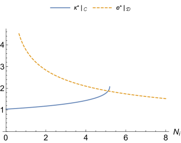
By contrast, the fixed-point value $\kappa^{\ast}$ at fixed point $\mathcal{C}$ increases with flavor number. Moreover, the fixed point disappears in a fixed-point collision at $N_{\text{i,cr}}^{\kappa}=5.195$. We conclude that the universality class defined by fixed point $\mathcal{C}$ and UV-complete trajectories emanating from it exist only at small values of $N_{\text{i}}$. This suggests that the universality class, its property of asymptotic safety, as well as possible quantum phase transitions induced in the long-range properties are not visible in a large-$N_{\text{f}}$ expansion. We emphasize that the interesting case of $N_{\text{f}}=2$ and $d_{\gamma}=4$, i.e., $N_{\text{i}}=4$–discussed in the context of high-$T_{\text{c}}$ cuprate superconductors or graphene–is below the critical flavor number $N_{\text{i,cr}}^{\kappa}$. We list our quantitative results for the fixed-point properties for this important case in Tab. 3.

	$e$	$\kappa$	$m$	multiplicity	$n_{\mathrm{phys}}$	$\theta_{\mathrm{max}}$	$\eta_{\psi}$	$\eta_{\mathrm{A}}$
$\mathcal{A:}$	$0$	$0$	$0$	$-$	$2$	$1.00$	$0.00$	$0.00$
$\mathcal{C:}$	$0$	$1.44$	$0$	$\mathbb{Z}_{2}$	$3$	$1.05$	$-0.716$	$0.876$
$\mathcal{D:}$	$2.10$	$0$	$0$	$\mathbb{Z}_{2}$	$1$	$1.64$	$-0.156$	$0.946$

Table 3: Fixed points of $d=3$ dimensional QED for $N_{\text{f}}=2$ flavors of reducible fermions $d_{\gamma}=4$, i.e., $N_{\text{i}}=4$.

The finite range of flavor numbers for which $\mathcal{C}$ exists can accommodate several scenarios depending on the value of the critical flavor number $N_{\text{i,cr}}^{\chi}$ below which chiral symmetry breaking occurs as potentially triggered by a large gauge coupling near fixed point $\mathcal{D}$. If $N_{\text{i,cr}}^{\chi}<N_{\text{i,cr}}^{\kappa}$, then there is a finite window where the system can flow from $\mathcal{C}$ in the UV to $\mathcal{D}$ in the IR along a separatrix. Let us for the moment assume that the case $N_{\text{i}}=4$, i.e., $N_{\text{f}}=2$ for reducible fermions $d_{\gamma}=4$, is inside this conformal window. Then there must be at least one trajectory that connects the two fixed points. If the system evolves along this trajectory from the UV to the IR, it would constitute an example of emerging chiral symmetry in the long-range properties of the theory. The reason is that the UV regime characterized by fixed point $\mathcal{C}$ corresponds to a universality class without chiral symmetry: the Pauli coupling violates chiral symmetry explicitly. By contrast, fixed point $\mathcal{D}$ is characterized by $m^{\ast}=0=\kappa^{\ast}=0$ and thus represents a chirally symmetric universality class.

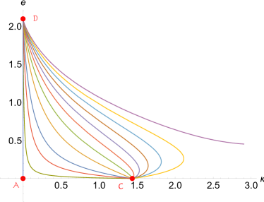
Of course, the mass direction is still a relevant perturbation at fixed point $\mathcal{D}$. Since fixed point $\mathcal{D}$ has two irrelevant directions in our approximation, a two-dimensional plane of trajectories must exist that end exactly in $\mathcal{D}$ and thus in a state of exact chiral symmetry. From the UV perspective, fixed point $\mathcal{C}$ has three relevant directions; hence, one of them needs to be fine-tuned in order for a trajectory to end in the chiral plane at fixed point $\mathcal{D}$. A projection of this one-parameter family onto the $(\kappa,e)$ plane is depicted in Fig. 6. Figure 7 further focuses on the running couplings and mass for a typical trajectory. We observe that the transition from the strong-Pauli-coupling regime to the long-range value of the gauge coupling coincides with the generation of a finite explicit mass which nonetheless subsides in the IR. For comparison, we also show an analogous trajectory from the Gaussian fixed point $\mathcal{A}$ to $\mathcal{D}$.

Figure 6: One-parameter family of RG trajectories projected onto the $(\kappa,e)$ plane for $N_{i}=4$ irreducible flavor degrees of freedom in $d=3$ spacetime dimensions. These lead from the fully repulsive UV fixed point $\mathcal{C}$ to the IR fixed point $\mathcal{D}$ at $\kappa^{*}=m^{*}=0$, thus exhibiting emergent chiral symmetry.

Figure 7: RG flow from the fully repulsive UV fixed point $\mathcal{C}$ to the IR fixed point $\mathcal{D}$ for $N_{i}=4$ irreducible flavor degrees of freedom in $d=3$ spacetime dimensions; initial conditions are chosen such that the mass parameter is zero in the UV and IR. For comparison, the trajectory from the Gaussian fixed point $\mathcal{A}$ to $\mathcal{D}$ is also shown (gray).

V Pauli-term fixed points in higher dimensions

Whereas the search for fixed points in higher dimensions may not offer an immediate physical implication, their study illustrates a mechanism underlying the existence of the fixed points investigated so far: namely, the competition between canonical scaling and quantum fluctuations. Towards higher dimensions, the gauge coupling which is marginal in $d=4$ becomes power-counting irrelevant, while the power-counting irrelevance of the Pauli coupling is further enhanced. The existence of non-Gaussian fixed-points thus requires similarly enhanced contributions from quantum fluctuations. If the latter contributions are bounded for some reason, we expect the non-Gaussian fixed points to disappear towards higher dimensions.

In the present case, we observe that the power-counting irrelevance of the gauge coupling $e$ is not counter-balanced by the fluctuation terms which further contribute to RG irrelevance. Hence, no fixed point is found on the $e$ axis apart from the Gaussian fixed point. In fact, slightly above $d=4$ dimensions, the fixed-point structure of $d=4$ as shown in Fig. 1 persists, but fixed points $\mathcal{B}$ and $\mathcal{C}$ approach each other. At a critical dimension $d_{\text{cr}}\simeq 4.27$ for $N_{\text{f}}=1$, the fixed point $\mathcal{C}$ collides with fixed point $\mathcal{B}$ (and its $\mathbb{Z}_{2}$ reflection), such that only one fixed point which we call $\mathcal{C}^{\prime}$ remains on the $\kappa$ axis. As a consequence of the fixed-point collision, the new fixed point $\mathcal{C}^{\prime}$ has one relevant direction (and thus one physical parameter) fewer than $\mathcal{C}$. Towards higher dimensions, $\mathcal{C}^{\prime}$ moves towards larger values of $\kappa$ and the anomalous dimensions grow beyond $\mathcal{O}(1)$.

Towards larger values of $N_{\text{f}}$, we observe only quantitative changes, but the picture remains qualitatively the same. For instance, for $N_{\text{f}}=10$, the collision of $\mathcal{B}$ and $\mathcal{C}$ occurs at $d_{\text{cr}}\simeq 4.69$. This number increases beyond $d=5$ for even larger $N_{\text{f}}$. The fixed-point value of the Pauli coupling at $\mathcal{C}^{\prime}$ slightly decreases for larger $N_{\text{f}}$, but the anomalous dimensions remain rather large, cf. Tab.4.

	$N_{\text{f}}$	$e$	$\kappa$	$m$	multiplicity	$n_{\mathrm{phys}}$	$\theta_{\mathrm{max}}$	$\eta_{\psi}$	$\eta_{\mathrm{A}}$
$\mathcal{A:}$	$\forall$	$0$	$0$	$0$	$-$	$1$	$1.00$	$0.00$	$0.00$
$\mathcal{C}^{\prime}$:	1	$0$	$13.9$	$0$	$\mathbb{Z}_{2}$	$2$	$5.49$	$-2.17$	$-0.903$
$\mathcal{C}^{\prime}$:	5	$0$	$10.3$	$0$	$\mathbb{Z}_{2}$	$2$	$3.46$	$-1.05$	$-2.14$
$\mathcal{C}^{\prime}:$	10	$0$	$8.15$	$0$	$\mathbb{Z}_{2}$	$2$	$3.24$	$-0.623$	$-2.53$

Table 4: Fixed points of $d=5$ dimensional QED for various flavor numbers of irreducible fermions $d_{\gamma}=4$. Fixed point $\mathcal{C}^{\prime}$ is a remnant of a fixed-point collision. In view of the large anomalous dimensions, we interpret fixed point $\mathcal{C}^{\prime}$ as an artifact of the approximation (indicated by the gray font).

Since fixed point $\mathcal{C}^{\prime}$ with its large anomalous dimensions does not fully meet our consistency criteria, we consider $\mathcal{C}^{\prime}$ in $d=5$ as an artifact of our approximation. We interpret these findings as indicating that an asymptotic-safety scenario for QED induced by the Pauli term may not exist in higher dimensions $d=5,6,\dots$.

VI Conclusions

We have studied the renormalization flow of QED upon the inclusion of a Pauli spin-field coupling in general dimensions and flavor numbers. Using the functional RG for a nonperturbative estimate of the $\beta$ functions of the investigated couplings, we explore the fixed-point structure of the theory within a derivative expansion of the effective action. We specifically investigate the fate of UV-stable fixed points recently discovered in $d=4$ spacetime dimensions for $N_{\text{f}}=1$ and follow their evolution in theory space as a function of the number of dimensions and fermion flavors. Such fixed points serve to construct a UV-complete version of QED within an asymptotic-safety scenario. They define universality classes that govern the physical properties of the theory in the long-range limit.

Going away from $d=4$ dimensions, we observe the general trend that increasing the flavor number tends to destabilize the non-Gaussian fixed points discovered in four spacetime dimensions. The most promising candidate for a physically relevant universality class is the non-Gaussian fixed point at finite Pauli spin-field coupling but vanishing gauge coupling, termed fixed point $\mathcal{C}$, which also exists in $d=3$ dimensions for sufficiently small flavor numbers while satisfying the self-consistency criteria of our approximation. In particular, we observe this fixed-point for flavor numbers which are of relevance for effective theories of layered condensed-matter systems. This universality class may be of interest as it serves as an example where the microscopic theory exhibits explicit chiral symmetry breaking, but the long-range effective theory may still show a gapless phase protected by an emergent chiral symmetry. We explicitly construct RG trajectories that emanate from the non-Gaussian fixed point $\mathcal{C}$ and approach a long-range regime that is governed by the IR-attractive interacting fixed point in the gauge coupling known in the QED₃ literature. Depending on the flavor number, the latter may correspond to a strongly coupled IR phase characterized by spontaneous (or dynamical) chiral symmetry breaking, as is subject to an ongoing debate in the literature.

It is also interesting to observe that the fixed-point scenario found in $d=4$ does not analogously persist above four dimensions. A fixed-point collision modifies the phase structure at a critical flavor dimension which is in between $d=4$ and $d=5$ for small to moderate flavor numbers, but beyond $d=5$ for large flavor numbers. In either case, the fixed point observed in $d=5$ no longer meets the quality criteria of our approximation, implying that we do not find reliable evidence for a UV completion of QED within an asymptotic safety scenario in higher dimensions.

These findings represent an instructive example for the fact that UV completion through asymptotic safety requires a delicate balance of dimensional (canonical) scaling and quantum contributions to scaling. Simply adding higher-order operators to the truncated effective action is not sufficient to induce non-Gaussian fixed points–at least not in the computationally controllable part of theory space. This makes the evidence for the UV completion of QED exploiting the Pauli coupling as found in [9] even more remarkable as it is somewhat special to $d=4$. It does not analogously exist in higher dimensions, and extends to $d=3$ only for small flavor numbers.

Finally, the important question persists as to whether the strong Pauli coupling at the fixed point exerts a relevant influence on higher-dimensional operators such as four-fermion interactions. The latter are known to be crucial for the status of chiral symmetry in strongly interacting QED both in $d=3$ as well as $d=4$ dimensions. This is left for future work.

Appendix A $\beta$ functions

The quantum contributions to the beta functions along with the anomalous dimensions of the fields were computed in [9] and are summarized as follows.

$$\Delta\beta_{e} =-4v_{d}\frac{\left(d-4\right)\left(d-1\right)}{d}e^{3}\;l_{d}^{(1,\mathrm{B},\tilde{\mathrm{F}}^{2})}(0,m^{2})-16v_{d}\frac{\left(d-2\right)\left(d-1\right)}{d}e\kappa^{2}\;l_{d}^{(2,\mathrm{B},\tilde{\mathrm{F}}^{2})}(0,m^{2})$$

$$\phantom{=}-32v_{d}\frac{d-1}{d}e^{2}\kappa m\;l_{d}^{(1,\mathrm{B},\mathrm{F},\tilde{\mathrm{F}})}(0,m^{2},m^{2})-4v_{d}\frac{\left(d-2\right)\left(d-1\right)}{d}e^{3}m^{2}\;l_{d}^{(\mathrm{B},\mathrm{F}^{2})}(0,m^{2})$$

$$\phantom{=}-16v_{d}\frac{\left(d-4\right)\left(d-1\right)}{d}e\kappa^{2}m^{2}\;l_{d}^{(2,\mathrm{B},\mathrm{F}^{2})}(0,m^{2})$$ (14)

$$\Delta\beta_{\kappa} =16v_{d}\frac{\left(d-4\right)\left(d-1\right)}{d}\kappa^{3}\;l_{d}^{(2,\mathrm{B},\tilde{\mathrm{F}}^{2})}(0,m^{2})-4v_{d}\left(3\frac{\left(d-6\right)\left(d-2\right)}{d}+1\right)e^{2}\kappa\;l_{d}^{(1,\mathrm{B},\tilde{\mathrm{F}}^{2})}(0,m^{2})$$

$$\phantom{=}+4v_{d}\,e^{3}m\;\left[\frac{d-3}{d}\left(l_{d}^{(1,\mathrm{B},\tilde{\mathrm{F}}_{1},\mathrm{F})}(0,m^{2},m^{2})-l_{d}^{(1,\mathrm{B},\mathrm{F}_{1},\tilde{\mathrm{F}})}(0,m^{2},m^{2})\right)-\frac{\left(d-4\right)\left(d-1\right)}{2d}l_{d}^{(\mathrm{B},\mathrm{F},\tilde{\mathrm{F}})}(0,m^{2},m^{2})\right]$$

$$\phantom{=}+16v_{d}\;e\kappa^{2}m\;\left[\frac{5\left(d-4\right)\left(d-3\right)}{2d}\;l_{d}^{(1,\mathrm{B},\mathrm{F},\tilde{\mathrm{F}})}(0,m^{2},m^{2})+\frac{d-3}{d}\;l_{d}^{(2,\mathrm{B},\mathrm{F},\tilde{\mathrm{F}}_{1})}(0,m^{2},m^{2})\right]$$

$$\phantom{=}+16v_{d}\;e\kappa^{2}m\;\left[-\frac{d-3}{d}\;l_{d}^{(2,\mathrm{B},\mathrm{F}_{1},\tilde{\mathrm{F}})}(0,m^{2},m^{2})-\frac{d+2}{d}\;l_{d}^{(1,\mathrm{B},\mathrm{F},\tilde{\mathrm{F}})}(0,m^{2},m^{2})\right]$$

$$\phantom{=}+16v_{d}\left(1-\frac{\left(d-4\right)^{2}}{d}\right)\kappa^{3}m^{2}\;l_{d}^{(1,\mathrm{B},\mathrm{F}^{2})}(0,m^{2})+4v_{d}\frac{\left(d-4\right)\left(d-1\right)}{d}e^{2}\kappa m^{2}\;l_{d}^{(\mathrm{B},\mathrm{F}^{2})}(0,m^{2})$$ (15)

$$\Delta\beta_{m} =-16v_{d}\left(d-1\right)e\kappa\;l_{d}^{(1,\mathrm{B},\tilde{\mathrm{F}})}(0,m^{2})+16v_{d}\left(d-1\right)m\kappa^{2}\;l_{d}^{(1,\mathrm{B},\mathrm{F})}(0,m^{2})-4v_{d}\left(d-1\right)e^{2}m\;l_{d}^{(\mathrm{B},\mathrm{F})}(0,m^{2})$$ (16)

$$\eta_{\psi} =4v_{d}\frac{\left(d-2\right)\left(d-1\right)}{d}e^{2}\;l_{d}^{(\mathrm{B},\tilde{\mathrm{F}})}(0,m^{2})-8v_{d}\frac{d-1}{d}e^{2}\;l_{d}^{(1,\mathrm{B},\tilde{\mathrm{F}}_{1})}(0,m^{2})+16v_{d}\frac{\left(d-4\right)\left(d-1\right)}{d}\kappa^{2}\;l_{d}^{(1,\mathrm{B},\tilde{\mathrm{F}})}(0,m^{2})$$

$$\phantom{=}-32v_{d}\frac{d-1}{d}\kappa^{2}\;l_{d}^{(2,\mathrm{B},\tilde{\mathrm{F}}_{1})}(0,m^{2})+32v_{d}\frac{d-1}{d}e\kappa m\;l_{d}^{(1,\mathrm{B},\mathrm{F}_{1})}(0,m^{2})$$ (17)

$$\eta_{A} =8v_{d}\frac{d_{\gamma}N_{\text{f}}}{d+2}e^{2}\;l_{d}^{(2,\tilde{\mathrm{F}}_{1}^{2})}(m^{2})+16v_{d}d_{\gamma}N_{\text{f}}\kappa^{2}m^{2}l_{d}^{(\mathrm{F}^{2})}(m^{2})-16v_{d}\frac{d-4}{d}d_{\gamma}N_{\text{f}}\kappa^{2}\;l_{d}^{(1,\tilde{\mathrm{F}}^{2})}(m^{2})$$

$$\phantom{=}-64v_{d}\frac{d_{\gamma}N_{\text{f}}}{d}e\kappa m\;l_{d}^{(1,\tilde{\mathrm{F}},\mathrm{F}_{1})}(m^{2},m^{2})+8v_{d}\frac{d_{\gamma}N_{\text{f}}}{d}e^{2}m^{2}\;l_{d}^{(1,\mathrm{F}_{1}^{2})}(m^{2})$$ (18)

The threshold functions $l_{\dots}^{\dots}$ are defined according to the convention introduced in [9]:

$$l_{d}^{([n],X_{[x_{d}]}^{[x_{p}]},Y_{[y_{d}]}^{[y_{p}]},...)}(\omega_{X},\omega_{Y},...;\eta_{X},\eta_{Y},...) =\left(-1\right)^{1+x_{d}\,x_{p}+y_{d}\,y_{p}+...}\frac{k^{-2n-d+2x_{p}\left(1+x_{d}\right)+2y_{p}\left(1+y_{d}\right)+...}}{4v_{d}}$$ (19)

$$\phantom{=}\times\int\frac{\mathrm{d}^{d}p}{\left(2\pi\right)^{d}}\left(p^{2}\right)^{n}\tilde{\partial}_{t}\left[\left(\frac{\partial}{\partial p^{2}}\right)^{x_{d}}G_{X}(\omega_{X})\right]^{x_{p}}\left[\left(\frac{\partial}{\partial p^{2}}\right)^{y_{d}}G_{Y}(\omega_{Y})\right]^{y_{p}}\dots$$

Parameters in brackets are optional and are understood to have defaults: $n=0,x_{d}=0,y_{d}=0,\dots,x_{p}=1,y_{p}=1,\dots$. The sign conventions are such that all threshold functions are positive for finite mass parameters $\omega_{X,Y,\dots}$ and vanishing anomalous dimensions $\eta_{X,Y,\dots}$. As is conventional in the literature, the modified scale derivative is understood to act only on the regulator terms. The quantity $G_{X}(\omega)$ denotes the inverse regularized propagator of type $X$, i.e.,

$$G_{\mathrm{B}}(\omega)=\frac{1}{P_{\mathrm{B}}+\omega k^{2}},\quad P_{\mathrm{B}}=p^{2}\left[1+r_{\mathrm{B}}\left(\frac{p^{2}}{k^{2}}\right)\right],$$ (20)

$$G_{\mathrm{F}}(\omega) = \frac{1}{P_{\mathrm{F}}+\omega k^{2}},\quad P_{\mathrm{F}}=p^{2}\left[1+r_{\mathrm{F}}\left(\frac{p^{2}}{k^{2}}\right)\right]^{2}\!\!,$$ (21)

$$G_{\tilde{\mathrm{F}}}(\omega) = \frac{1+r_{\mathrm{F}}}{P_{\mathrm{F}}+\omega k^{2}},$$ (22)

where $r_{\mathrm{B}}$ and $r_{\mathrm{F}}$ are the boson and fermion regulator shape functions respectively. More details along with some explicitly computed threshold functions can be found in [9].

References

- Jackiw [2000] R. Jackiw, Int. J. Mod. Phys. B 14, 2011 (2000), arXiv:hep-th/9903044 .
- Zinn-Justin [1989] J. Zinn-Justin, Int. Ser. Monogr. Phys. 77, 1 (1989).
- Peskin and Schroeder [1995] M. E. Peskin and D. V. Schroeder, An Introduction to quantum field theory (1995).
- Schwinger [1948] J. S. Schwinger, Phys. Rev. 73, 416 (1948).
- Schwinger [1951] J. S. Schwinger, Phys. Rev. 82, 664 (1951).
- Laporta and Remiddi [1996] S. Laporta and E. Remiddi, Phys. Lett. B 379, 283 (1996), arXiv:hep-ph/9602417 .
- Aoyama et al. [2015] T. Aoyama, M. Hayakawa, T. Kinoshita, and M. Nio, Phys. Rev. D 91, 033006 (2015), [Erratum: Phys.Rev.D 96, 019901 (2017)], arXiv:1412.8284 [hep-ph] .
- Hanneke et al. [2011] D. Hanneke, S. F. Hoogerheide, and G. Gabrielse, Phys. Rev. A 83, 052122 (2011), arXiv:1009.4831 [physics.atom-ph] .
- Gies and Ziebell [2020] H. Gies and J. Ziebell, Eur. Phys. J. C 80, 607 (2020), arXiv:2005.07586 [hep-th] .
- Weinberg [1976] S. Weinberg, in Erice Subnucl.Phys.1976:1 (1976) p. 1.
- Weinberg [1980] S. Weinberg, in General Relativity: An Einstein Centenary Survey (1980) pp. 790–831.
- Landau [1955] L. D. Landau, in Niels Bohr and the Development of Physics, ed. Wolfgang Pauli, London: Pergamon Press (1955).
- Djukanovic et al. [2017] D. Djukanovic, J. Gegelia, and U.-G. Meißner, (2017), arXiv:1706.10039 [hep-th] .
- Gockeler et al. [1998] M. Gockeler, R. Horsley, V. Linke, P. E. L. Rakow, G. Schierholz, and H. Stuben, Phys. Rev. Lett. 80, 4119 (1998), arXiv:hep-th/9712244 [hep-th] .
- Gies and Jaeckel [2004] H. Gies and J. Jaeckel, Phys. Rev. Lett. 93, 110405 (2004), arXiv:hep-ph/0405183 [hep-ph] .
- Cortijo et al. [2012] A. Cortijo, F. Guinea, and M. A. H. Vozmediano, J. Phys. A 45, 383001 (2012), arXiv:1112.2054 [cond-mat.mes-hall] .
- Vafek and Vishwanath [2014] O. Vafek and A. Vishwanath, Ann. Rev. Condensed Matter Phys. 5, 83 (2014), arXiv:1306.2272 [cond-mat.mes-hall] .
- Franz and Tesanovic [2001] M. Franz and Z. Tesanovic, Phys. Rev. Lett. 87, 257003 (2001), arXiv:cond-mat/0012445 .
- Franz et al. [2002] M. Franz, Z. Tesanovic, and O. Vafek, Phys. Rev. B 66, 054535 (2002), arXiv:cond-mat/0203333 .
- Herbut [2002a] I. F. Herbut, Phys. Rev. Lett. 88, 047006 (2002a), arXiv:cond-mat/0110188 .
- Herbut [2002b] I. F. Herbut, Phys. Rev. B 66, 094504 (2002b), arXiv:cond-mat/0202491 .
- Tesanovic et al. [2002] Z. Tesanovic, O. Vafek, and M. Franz, Phys. Rev. B 65, 180511 (2002), arXiv:cond-mat/0110253 .
- Mavromatos and Papavassiliou [2004] N. E. Mavromatos and J. Papavassiliou, Recent Res. Devel. Phys. 5, 369 (2004), arXiv:cond-mat/0311421 .
- Herbut [2005] I. F. Herbut, Phys. Rev. Lett. 94, 237001 (2005), arXiv:cond-mat/0410557 .
- Appelquist et al. [1988] T. Appelquist, D. Nash, and L. C. R. Wijewardhana, Phys. Rev. Lett. 60, 2575 (1988).
- Nash [1989] D. Nash, Phys. Rev. Lett. 62, 3024 (1989).
- Pennington and Walsh [1991] M. R. Pennington and D. Walsh, Phys. Lett. B 253, 246 (1991).
- Atkinson et al. [1990] D. Atkinson, P. W. Johnson, and P. Maris, Phys. Rev. D 42, 602 (1990).
- Curtis et al. [1992] D. C. Curtis, M. R. Pennington, and D. Walsh, Phys. Lett. B 295, 313 (1992).
- Ebihara et al. [1995] T. Ebihara, T. Iizuka, K.-i. Kondo, and E. Tanaka, Nucl. Phys. B 434, 85 (1995), arXiv:hep-ph/9404361 .
- Aitchison et al. [1997] I. J. R. Aitchison, N. E. Mavromatos, and D. McNeill, Phys. Lett. B 402, 154 (1997), arXiv:hep-th/9701087 .
- Appelquist et al. [1999] T. Appelquist, A. G. Cohen, and M. Schmaltz, Phys. Rev. D 60, 045003 (1999), arXiv:hep-th/9901109 .
- Gusynin and Reenders [2003] V. P. Gusynin and M. Reenders, Phys. Rev. D 68, 025017 (2003), arXiv:hep-ph/0304302 .
- Fischer et al. [2004] C. S. Fischer, R. Alkofer, T. Dahm, and P. Maris, Phys. Rev. D70, 073007 (2004), arXiv:hep-ph/0407104 [hep-ph] .
- Kaveh and Herbut [2005] K. Kaveh and I. F. Herbut, Phys. Rev. B 71, 184519 (2005), arXiv:cond-mat/0411594 .
- Kubota and Terao [2001] K.-i. Kubota and H. Terao, Prog. Theor. Phys. 105, 809 (2001), arXiv:hep-ph/0101073 .
- Hands et al. [2002] S. J. Hands, J. B. Kogut, and C. G. Strouthos, Nucl. Phys. B 645, 321 (2002), arXiv:hep-lat/0208030 .
- Hands et al. [2004] S. J. Hands, J. B. Kogut, L. Scorzato, and C. G. Strouthos, Phys. Rev. B 70, 104501 (2004), arXiv:hep-lat/0404013 .
- Mitra et al. [2007] I. Mitra, R. Ratabole, and H. S. Sharatchandra, Mod. Phys. Lett. A 22, 297 (2007), arXiv:hep-th/0601058 .
- Bashir et al. [2008] A. Bashir, A. Raya, I. C. Cloet, and C. D. Roberts, Phys. Rev. C 78, 055201 (2008), arXiv:0806.3305 [hep-ph] .
- Bashir et al. [2009] A. Bashir, A. Raya, S. Sanchez-Madrigal, and C. D. Roberts, Few Body Syst. 46, 229 (2009), arXiv:0905.1337 [hep-ph] .
- Feng et al. [2012] H.-t. Feng, B. Wang, W.-m. Sun, and H.-s. Zong, Phys. Rev. D 86, 105042 (2012).
- Grover [2014] T. Grover, Phys. Rev. Lett. 112, 151601 (2014), arXiv:1211.1392 [hep-th] .
- Braun et al. [2014] J. Braun, H. Gies, L. Janssen, and D. Roscher, Phys. Rev. D90, 036002 (2014), arXiv:1404.1362 [hep-ph] .
- Raviv et al. [2014] O. Raviv, Y. Shamir, and B. Svetitsky, Phys. Rev. D 90, 014512 (2014), arXiv:1405.6916 [hep-lat] .
- Karthik and Narayanan [2015] N. Karthik and R. Narayanan, Phys. Rev. D 92, 025003 (2015), arXiv:1505.01051 [hep-th] .
- Di Pietro et al. [2016] L. Di Pietro, Z. Komargodski, I. Shamir, and E. Stamou, Phys. Rev. Lett. 116, 131601 (2016), arXiv:1508.06278 [hep-th] .
- Giombi et al. [2016] S. Giombi, I. R. Klebanov, and G. Tarnopolsky, J. Phys. A 49, 135403 (2016), arXiv:1508.06354 [hep-th] .
- Chester and Pufu [2016] S. M. Chester and S. S. Pufu, JHEP 08, 019 (2016), arXiv:1601.03476 [hep-th] .
- Janssen [2016] L. Janssen, Phys. Rev. D 94, 094013 (2016), arXiv:1604.06354 [hep-th] .
- Herbut [2016] I. F. Herbut, Phys. Rev. D 94, 025036 (2016), arXiv:1605.09482 [hep-th] .
- Karthik and Narayanan [2016] N. Karthik and R. Narayanan, Phys. Rev. D 94, 065026 (2016), arXiv:1606.04109 [hep-th] .
- Gusynin and Pyatkovskiy [2016] V. P. Gusynin and P. K. Pyatkovskiy, Phys. Rev. D 94, 125009 (2016), arXiv:1607.08582 [hep-ph] .
- Gukov [2017] S. Gukov, Nucl. Phys. B 919, 583 (2017), arXiv:1608.06638 [hep-th] .
- Goswami et al. [2017] P. Goswami, H. Goldman, and S. Raghu, Phys. Rev. B 95, 235145 (2017), [Erratum: Phys.Rev.B 99, 079903 (2019)], arXiv:1701.07828 [cond-mat.str-el] .
- Janssen and He [2017] L. Janssen and Y.-C. He, Phys. Rev. B 96, 205113 (2017), arXiv:1708.02256 [cond-mat.str-el] .
- Di Pietro and Stamou [2017] L. Di Pietro and E. Stamou, JHEP 12, 054 (2017), arXiv:1708.03740 [hep-th] .
- Ihrig et al. [2018] B. Ihrig, L. Janssen, L. N. Mihaila, and M. M. Scherer, Phys. Rev. B 98, 115163 (2018), arXiv:1807.04958 [cond-mat.str-el] .
- Benvenuti and Khachatryan [2018] S. Benvenuti and H. Khachatryan, (2018), arXiv:1812.01544 [hep-th] .
- Li [2018] Z. Li, (2018), arXiv:1812.09281 [hep-th] .
- Albayrak et al. [2022] S. Albayrak, R. S. Erramilli, Z. Li, D. Poland, and Y. Xin, Phys. Rev. D 105, 085008 (2022), arXiv:2112.02106 [hep-th] .
- Gies [2003] H. Gies, Phys. Rev. D68, 085015 (2003), arXiv:hep-th/0305208 [hep-th] .
- Morris [2005] T. R. Morris, JHEP 01, 002 (2005), arXiv:hep-ph/0410142 .
- de Forcrand et al. [2010] P. de Forcrand, A. Kurkela, and M. Panero, JHEP 06, 050 (2010), arXiv:1003.4643 [hep-lat] .
- Knechtli and Rinaldi [2016] F. Knechtli and E. Rinaldi, Int. J. Mod. Phys. A 31, 1643002 (2016), arXiv:1605.04341 [hep-lat] .
- Codello et al. [2016] A. Codello, K. Langæble, D. F. Litim, and F. Sannino, JHEP 07, 118 (2016), arXiv:1603.03462 [hep-th] .
- Eichhorn et al. [2016] A. Eichhorn, L. Janssen, and M. M. Scherer, (2016), arXiv:1604.03561 [hep-th] .
- Gracey et al. [2018] J. A. Gracey, I. F. Herbut, and D. Roscher, Phys. Rev. D 98, 096014 (2018), arXiv:1810.05721 [hep-th] .
- Fischer and Litim [2006] P. Fischer and D. F. Litim, Phys. Lett. B 638, 497 (2006), arXiv:hep-th/0602203 .
- Falls [2015] K. Falls, Phys. Rev. D 92, 124057 (2015), arXiv:1501.05331 [hep-th] .
- Gies et al. [2015] H. Gies, B. Knorr, and S. Lippoldt, (2015), arXiv:1507.08859 [hep-th] .
- Eichhorn and Schiffer [2019] A. Eichhorn and M. Schiffer, Phys. Lett. B 793, 383 (2019), arXiv:1902.06479 [hep-th] .
- Weinberg [1960] S. Weinberg, Phys. Rev. 118, 838 (1960).
- Aoki et al. [1997] K.-I. Aoki, K.-i. Morikawa, J.-I. Sumi, H. Terao, and M. Tomoyose, Prog. Theor. Phys. 97, 479 (1997), arXiv:hep-ph/9612459 .
- Gies and Jaeckel [2006] H. Gies and J. Jaeckel, Eur. Phys. J. C46, 433 (2006), arXiv:hep-ph/0507171 [hep-ph] .
- Braun and Gies [2006] J. Braun and H. Gies, JHEP 06, 024 (2006), arXiv:hep-ph/0602226 [hep-ph] .
- Herbut [2006] I. F. Herbut, Phys. Rev. Lett. 97, 146401 (2006), arXiv:cond-mat/0606195 [cond-mat] .
- Wetterich [1993] C. Wetterich, Phys. Lett. B301, 90 (1993).
- Bonini et al. [1993] M. Bonini, M. D’Attanasio, and G. Marchesini, Nucl. Phys. B409, 441 (1993), arXiv:hep-th/9301114 [hep-th] .
- Ellwanger [1994] U. Ellwanger, Proceedings, Workshop on Quantum field theoretical aspects of high energy physics: Bad Frankenhausen, Germany, September 20-24, 1993, Z. Phys. C62, 503 (1994), [,206(1993)], arXiv:hep-ph/9308260 [hep-ph] .
- Morris [1994] T. R. Morris, Int. J. Mod. Phys. A9, 2411 (1994), arXiv:hep-ph/9308265 [hep-ph] .
- Litim [2000] D. F. Litim, Phys. Lett. B486, 92 (2000), arXiv:hep-th/0005245 [hep-th] .
- Litim [2001] D. F. Litim, Phys. Rev. D64, 105007 (2001), arXiv:hep-th/0103195 [hep-th] .
- Pisarski [1984] R. D. Pisarski, Phys. Rev. D 29, 2423 (1984).
- Stam [1986] K. Stam, Phys. Rev. D 34, 2517 (1986).
- O’Dwyer and Osborn [2008] J. O’Dwyer and H. Osborn, Annals Phys. 323, 1859 (2008), arXiv:0708.2697 [hep-th] .
- Codello et al. [2018] A. Codello, M. Safari, G. P. Vacca, and O. Zanusso, Eur. Phys. J. C78, 30 (2018), arXiv:1705.05558 [hep-th] .
- Codello et al. [2017] A. Codello, M. Safari, G. P. Vacca, and O. Zanusso, JHEP 04, 127 (2017), arXiv:1703.04830 [hep-th] .
- Martini and Zanusso [2019] R. Martini and O. Zanusso, Eur. Phys. J. C 79, 203 (2019), arXiv:1810.06395 [hep-th] .