Adjoint-based Control of Three Dimensional Stokes Droplets

Abstract

We develop a continuous adjoint formulation and implementation for controlling the deformation of clean, neutrally buoyant droplets in Stokes flow through farfield velocity boundary conditions. The focus is on dynamics where surface tension plays an important role through the Young-Laplace law. To perform the optimization, we require access to first-order gradient information, which we obtain from the linearized sensitivity equations and their corresponding adjoint by applying shape calculus to the space-time tube formed by the interface evolution. We show that the adjoint evolution equation can be efficiently expressed through a scalar adjoint transverse field. The optimal control problem is discretized by high-order boundary integral methods using Quadrature by Expansion coupled with a spherical harmonic representation of the droplet surface geometry. We show the accuracy and stability of the scheme on several tracking-type control problems.

Ox  d #1 m #1 m m d #1d #2 m m ∂#1∂#2 sm #1 ⟨#2 ⟩ ⟨#2 ⟩ sm #1 ⟨#2 ⟩ ⟨#2 ⟩ sm #1 ⟨#2 ⟩ ⟦#2 ⟧ O1 m m m m exampleExamplesection remarkRemarksection definitionDefinitionsection propositionPropositionsection lemmaLemmasection theoremTheoremsection

1 Introduction

In many droplet-based microfluidic processes and applications, the precise shape and position of the droplets over time plays a significant role in the performance and efficiency of the system. A standard simplified model for such problems consists of the two-phase Stokes equations coupled with interfacial forces (surface tension) or additional surfactants and gravity (several concrete examples can be found in [1]). Optimizing aspects of this type of system is our focus. However, other types of interface evolution share similar features, e.g. mean curvature flows [2, 3], fluid-structure interactions or free surface flows, and can be analyzed by similar methods.

In general, the application of the continuous or discrete adjoint method to the field of optimal control has been very successful, with applications to fluid mechanics starting from [4]. However, applications to two-phase flows are rare due, in part, to the fact that the field itself remains an active area of research. Phase-field-type models present a compelling starting point, as the fields representing the flow quantities are smooth and classic approaches to adjoint methods can be applied. For example, in [5, 6, 7] the Cahn–Hilliard equations are coupled with the incompressible Navier–Stokes equations and the corresponding optimal control problem is solved. On the other-hand, sharp interface models (see [8]) are difficult to handle due to the discontinuities of the state variables and material quantities. Furthermore, incorporating interface jump conditions containing higher-order derivatives of the geometry (mainly curvature) is problematic, see [9]. Work on two-phase problems has also advanced in recent years, with applications to fluid-structure interactions [10], two-phase Stefan equations [11], free-surface flows [12, 13], geometric flows [14, 15], etc. Initial extensions to the incompressible two-phase Navier–Stokes with Volume-of-Fluid formulation are presented in [16, 17].

In this paper, we extend the work presented initially in [18]. The focus of the previous work was on the optimal control of a single droplet under axisymmetric assumptions. We relax these assumptions and extend the applications to fully three-dimensional problems with multiple droplets. While applications to scenarios of practical interest, where hundreds or thousands of droplets are present in the system, are still prohibitively expensive, we present several improvements. First, we show that the vector adjoint evolution equation from [18] can be transformed into a scalar evolution equation for the normal component only. This is a significant reduction in cost, especially in three dimensions. Furthermore, we make use of state-of-the art methods for solving boundary integral equations to improve the general performance of the Stokes solver itself. In this work, the Quadrature by Expansion method [19] is used, for which accurate Fast Multipole Methods have been developed [20]. This allows constructing a fast solver that scales approximately linearly in the number of degrees of freedom.

The outline of the paper is as follows. We start in Section 2 with a description of the two-phase control problem, focusing on the constraints and the cost functional. In Section 3, we present the main ideas behind applying shape calculus to PDEs on moving domains. These concepts are applied to deriving the linearized and adjoint equations for the control problem. In Section 4, we present a discretization of the state and adjoint systems through a coupled representation by boundary integral methods (for the Stokes problem) and spherical harmonics (for the geometry). Finally, Section 5 presents several verification tests and applications to three-dimensional multi-droplet systems. We conclude with some remarks in Section 6.

2 Control of Two-Phase Stokes Flow

In this paper we will consider the evolution of a system of droplets in an otherwise infinite domain. To this end, we define an open finite domain $\Omega_{-}\subset\mathbb{R}^{d}$, where $d=3$, and its complement $\Omega_{+}\triangleq\mathbb{R}^{d}\setminus\bar{\Omega}_{-}$ to denote the interior of the droplets and the surrounding fluid, respectively. The droplet surface $\Sigma\triangleq\bar{\Omega}_{+}\cap\bar{\Omega}_{+}$ is assumed to be a finite set of disjoint, closed, bounded, and orientable surfaces at each instance of time (see Figure 1).

Figure 1: Example droplet configuration.

The interface $\Sigma(t)$ is the focus in the control of two-phase flows. As such, we define $\mathcal{D}\subset\mathbb{R}^{d}$ as a bounded open set which will contain all admissible interface configurations $\Sigma(t)$ for our problem. The general optimization problem we will be looking at pertains to evolutions equations of the form

$$\begin{cases}\dot{\vect{X}}=\vect{V}(t,\vect{X}(t),\vect{g}),&\quad t\in[0,T],\\ \vect{X}(0)=\vect{X}_{0},\end{cases}$$ (1)

where $\vect{X}(t)\in\mathcal{D}$ is a parametrization of the interface $\Sigma(t)$ and $\vect{g}$ represents a chosen control. For sufficiently smooth right-hand sides, we can define a transformation $\vect{T}(\vect{V}):\mathcal{D}\to\mathcal{D}$ by $\vect{X}(t)=\vect{T}(\vect{V})(\vect{X}_{0})$ for every flow $\vect{V}$. We can then follow the results from [21] to derive evolution equations for the linearized problem, the adjoint problem and ultimately an expression for the adjoint-based gradient. This will be discussed in detail in Section 3.

2.1 Quasi-static Two-Phase Stokes Flow

We consider the quasi-static evolution of multiple droplets in a viscous incompressible flow. The droplets experience no phase change, but are driven by surface tension forces at the fluid-fluid interface. In each phase, the fluid is described by the velocity fields $\vect{u}_{\pm}:\Omega_{\pm}\to\mathbb{R}^{d}$ and the pressures $p_{\pm}:\Omega_{\pm}\to\mathbb{R}_{+}$. Assuming a low-Reynolds number, the equations governing the flow are the two-phase Stokes equations

$$\begin{cases}\nabla\cdot\vect{u}_{\pm}=0,&\quad\vect{x}\in\Omega_{\pm}(t),\\ \nabla\cdot\sigma_{\pm}[\vect{u},p]=0,&\quad\vect{x}\in\Omega_{\pm}(t),\\ \vect{u}_{+}\to\vect{u}_{\infty}(\vect{g}),&\quad\|\vect{x}\|\to\infty,\end{cases}$$ (2)

where $\vect{u}_{\infty}$ defines an intended decay at infinity of the velocity field $\vect{u}_{+}$. The full velocity field $\vect{u}$ is to be understood as a superposition of $\vect{u}_{\infty}$ and a flow that decays to zero in the farfield. The Cauchy stress tensor $\sigma_{\pm}$ and the rate of strain tensor $\varepsilon_{\pm}$ are written as

$$\sigma_{\pm}[\vect{u},p]\triangleq -p_{\pm}I+2\mu_{\pm}\varepsilon_{\pm}[\vect{u}],$$

$$\varepsilon_{\pm}[\vect{u}]\triangleq \frac{1}{2}(\nabla\vect{u}_{\pm}+\nabla\vect{u}_{\pm}^{T}),$$

where $\mu_{\pm}\in\mathbb{R}_{+}$ are the dynamic viscosities of each fluid. We will assume that the surface forces are entirely due to a constant surface tension. The boundary conditions at the drop surface are the continuity of velocity and the Young-Laplace law, i.e.

$$\begin{cases}\jump{\vect{u}}=0,\\ \jump{\vect{n}\cdot\sigma[\vect{u},p]}=\gamma\kappa\vect{n},\end{cases}$$ (3)

where $\gamma$ is a constant surface tension coefficient, $\kappa$ is the total curvature (sum of the principal curvatures) and $\vect{n}$ is the exterior normal to $\Omega_{-}$. The jump at the interface is defined as

$$\jump{f}\triangleq f(\vect{x}_{+})-f(\vect{x}_{-}),\quad\text{where }f(\vect{x}_{\pm})\triangleq\lim_{\epsilon\to 0^{+}}f(\vect{x}\pm\epsilon\vect{n}).$$

The equations are non-dimensionalized by making use of a characteristic velocity magnitude $U$ and a characteristic droplet radius $R$. The resulting non-dimensional parameters are the viscosity ratio $\lambda$ and the Capillary number $\mathrm{Ca}$,

$$\lambda\triangleq\frac{\mu_{-}}{\mu_{+}}\quad\text{and}\quad\mathrm{Ca}\triangleq\frac{\mu_{+}U}{\gamma},$$

The non-dimensional equations will be used going forward. In this form, non-dimensional weighted jump and average operators are defined as

$$\jump{f}_{\lambda}\triangleq f(\vect{x}_{+})-\lambda f(\vect{x}_{-})\quad\text{and}\quad\avg{f}_{\lambda}\triangleq\frac{1}{2}(f(\vect{x}_{+})+\lambda f(\vect{x}_{-})).$$

In order to evolve the interface in time, we use a quasi-static approach in which we first compute the velocity from (2) and then displace the interface using the ODE from (1). For Stokes flow, the motion law is given by

$$\vect{V}(\vect{u},\vect{X})\triangleq(\vect{u}\cdot\vect{n})\vect{n}+(I-\vect{n}\otimes\vect{n})\vect{w},$$ (4)

which is well-defined since $\jump{\vect{u}}=0$ allows for a unique interface velocity field. At a continuous level, only the normal component of the velocity is necessary to define the deformation of the interface. Tangential components from $\vect{w}:[0,T]\times\mathbb{R}^{3}\to\mathbb{R}^{3}$ can be seen as reparametrizations and represent the same abstract shape. They become important in the discretization stage, as discussed in Section 4, and should be included in the adjoint to obtain accurate gradients.

2.2 Cost Functionals

Our goal is to find controls $\vect{g}$ (from (1)) that minimize a class of tracking-type cost functionals. The general form of the cost functionals we will be looking at is

$$J(\vect{g})\triangleq\frac{\alpha_{1}}{2}\int_{0}^{T}\int_{\Sigma(t)}(\vect{u}\cdot\vect{n}-u_{d})^{2}\dx[S]\dx[t]+\frac{\alpha_{2}}{2}\int_{0}^{T}\|\vect{x}_{c}(t)-\vect{x}_{d}(t)\|^{2}\dx[t]+\frac{\alpha_{3}}{2}\|\vect{x}_{c}(T)-\vect{x}_{d,T}\|^{2},$$ (5)

where $u_{d}$ is a target surface normal velocity field, while $\vect{x}_{d}(t)$ and $\vect{x}_{d,T}$ are target droplets centroids. We mainly consider the droplet centroids as a way to describe the position, but any quantity that is invariant to reparametrizations can be used. This assumption can be relaxed by considering reparametrizations as described in [22]. Then, we consider the optimization problem

$$\begin{cases}\min J(\vect{g}),\\ \text{subject to~{}\eqref{eq:evolution} (with~{}\eqref{eq:kinematic}), \eqref{eq:stokes} and~{}\eqref{eq:jumps}.}\end{cases}$$ (6)

The main control variable we will be focusing on are the farfield boundary conditions $\vect{u}_{\infty}(\vect{g})$. For finite domains, this is a straightforward choice. However, as the farfield boundary conditions are used to impose a decay in the velocity field, further discussion is required (see Section 3).

In the absence of an evolution equation, such as (1), we can consider a static system. In this case, the interface $\vect{X}$ becomes the control and we are left with a standard shape optimization problem. As shown in [18], the static problem is an important stepping stone in deriving and verifying the required optimality conditions. We will be making use of the static problem to verify the adjoint equations for the three-dimensional problem presented here as well.

3 Cost Gradients

To understand the optimization problem proposed by (6), we must introduce several important notions from shape calculus and more general perturbations of moving domains. These ideas are detailed in [21]. First, for an initial configuration $\Omega_{0}$ and interface $\Sigma_{0}$, we define the space-time tubes on $\mathbb{R}_{+}\times\mathbb{R}^{d}$, corresponding to a velocity field $\vect{V}$, by (see also Figure 2)

$$\Omega(\vect{V})\triangleq \bigcup_{t\in[0,T]}\{t\}\times\Omega(t)=\bigcup_{t\in[0,T]}\{t\}\times\vect{T}(\vect{V})(\Omega_{0}),$$

$$\Sigma(\vect{V})\triangleq \bigcup_{t\in[0,T]}\{t\}\times\Sigma(t)=\bigcup_{t\in[0,T]}\{t\}\times\vect{T}(\vect{V})(\Sigma_{0}).$$

Figure 2: Schematic of the (two-dimensional) $\Omega(\vect{V})$ and $\Sigma(\vect{V})$ space-times tubes and transverse slices $\Omega(t)$ (blue) and $\Sigma(t)$ (red) at fixed times $t$. The perturbations $\tilde{\vect{V}}$ only act in the transverse direction (gray slices).

A perturbation in the control $\vect{g}$ can then be seen as giving rise to a perturbed space-time tube $\Omega_{\epsilon}(\vect{V})$. Perturbations obtained in this way are called transverse because they occur only in “horizontal” slices of each $\Omega(t)$ domain for fixed $t$. This allows recovering most of the classic formulae from shape calculus in the context of moving domains. To clarify these ideas, we consider a perturbation of the control and the corresponding perturbation of the motion law, i.e.

$$\vect{g}_{\epsilon}= \vect{g}+\epsilon\tilde{\vect{g}},$$

$$\vect{V}_{\epsilon}(t,\vect{x};\vect{g})= \vect{V}(t,\vect{x};\vect{g})+\epsilon\vect{W}(t,\vect{x};\vect{g},\tilde{\vect{g}}),$$

for a specific $\vect{W}$ such that $\vect{W}(0,\vect{x};\vect{g},\tilde{\vect{g}})=\vect{0}$. The expression for $\vect{V}_{\epsilon}$ is valid under sufficient regularity assumptions and can be used to obtain first-order perturbations of the tube $\Omega(\vect{V})$. To obtain derivatives of the cost functional (5), we are interested in functionals of the form

$$J_{1}(\vect{V})\triangleq \int_{0}^{T}\int_{\Omega(t)}f(\vect{V})\dx[V]\dx[t],$$

$$J_{2}(\vect{V})\triangleq \int_{0}^{T}\int_{\Sigma(t)}g(\vect{V})\dx[S]\dx[t],$$

where $f,g:\Omega(t)\to\mathbb{R}$. From [21, Theorem 5.4, 5.5], we have that their directional derivatives are given by

$$DJ_{1}(\vect{V})[\vect{W}]= \int_{0}^{T}\int_{\Omega(t)}f^{\prime}(\vect{V})[\vect{W}]\dx[V]\dx[t]+\int_{0}^{T}\int_{\partial\Omega(t)}f(\vect{V})\tilde{\vect{V}}\cdot\vect{n}\dx[S]\dx[t],$$ (7)

$$DJ_{2}(\vect{V})[\vect{W}]= \int_{0}^{T}\int_{\Sigma(t)}g^{\prime}(\vect{V})[\vect{W}]\dx[S]\dx[t]+\int_{0}^{T}\int_{\Sigma(t)}(\vect{n}\cdot\nabla g+\kappa g)\tilde{\vect{V}}\cdot\vect{n}\dx[S]\dx[t],$$

where $f^{\prime}$ and $g^{\prime}$ denote the shape derivatives of $f$ and $g$, respectively, as defined in [21]. In classic shape calculus the perturbation $\tilde{\vect{V}}$ is taken as a direct perturbation of the geometry itself. However, for moving domains this perturbation satisfies an evolution equation of the form

$$\begin{cases}\tilde{\vect{V}}_{t}+(\vect{V}\cdot\nabla\tilde{\vect{V}}-\tilde{\vect{V}}\cdot\nabla\vect{V})=\vect{W},&\quad(t,\vect{X})\in[0,T]\times\mathcal{D},\\ \tilde{\vect{V}}(0,\vect{x})=\vect{0},&\quad\vect{x}\in\mathcal{D},\end{cases}$$ (8)

which ties it to the original perturbation $\vect{W}$ of the velocity field $\vect{V}$. The equation for the transverse field $\tilde{\vect{V}}$ is in fact an ODE if we consider the evolution under the path described by $\vect{X}(t)$ and driven by the velocity field $\vect{V}$ through (1). For a proof of this fact and additional considerations, we direct the reader to [15] or [21]. As the directional derivatives match those obtained by shape calculus on static domains, we make use of the results from [23] to express any additional shape derivatives for, e.g., the normal vector, the total curvature, etc.

3.1 Sensitivity Equations

A first step in solving the optimal control (6) consists in determining the sensitivity of the cost functional (5) with respect to the control. For this, we must consider the cost $J(\vect{g})$ as the composition of $\vect{g}\mapsto\vect{V}(\vect{g})$ and a shape functional $\vect{V}\mapsto J(\vect{V})$. For the shape functional, we can make use of the formulae provided in (7).

Therefore, it remains to find a transverse field equation (8) that links the perturbations of $\vect{g}$ to the transverse field $\tilde{\vect{V}}$ and incorporates the constraints given by the two-phase Stokes equations from (2). A similar problem was analyzed in [15], where a volume-preserving mean curvature flow was used as the motion law. Incorporating the two-phase Stokes equations requires a more careful approach, as we must deal with the discontinuous variables and jump conditions. To determine the linearized equations, we consider the weak formulation of the flow, as described in [18]. This weak formulation contains all the relevant terms and expresses the geometry dependence in an explicit way, as opposed to the strong form from (2). An introduction to these ideas and applications to simpler elliptic problems are given in [24].

We expand on [18] by introducing the tangential field $\vect{w}$ from (4) in the adjoint equations. A weak formulation of the kinematic condition is then given by

$$\inp{\dot{\vect{X}},\vect{Y}}_{\Sigma(t)}-\inp{(\vect{u}\cdot\vect{n})\vect{n},\vect{Y}}_{\Sigma(t)}-\inp{(I-\vect{n}\otimes\vect{n})\vect{w},\vect{Y}}_{\Sigma(t)}=0,$$

for all test functions $\vect{Y}\in L^{2}(\Sigma)$. The linearized equations are then obtained by perturbing the weak formulation using the shape derivatives from (7) and the transverse field equation (8). The linearized two-phase Stokes equations for the shape derivative $(p_{\pm}^{\prime},\vect{u}_{\pm}^{\prime})$ are given by

$$\begin{cases}\nabla\cdot\vect{u}_{\pm}^{\prime}=0,&\quad\vect{x}\in\Omega_{\pm}(t),\\ \nabla\cdot\sigma_{\pm}[\vect{u}^{\prime},p^{\prime}]=0,&\quad\vect{x}\in\Omega_{\pm}(t),\\ \vect{u}_{+}^{\prime}\to\vect{u}_{\infty}^{\prime}[\tilde{\vect{g}}],&\quad\|\vect{x}\|\to\infty,\end{cases}$$ (9)

with the jump conditions at the interface

$$\begin{cases}\jump{\vect{u}^{\prime}}=-\jump{\vect{n}\cdot\nabla\vect{u}}(\tilde{\vect{V}}\cdot\vect{n}),\\ \displaystyle\jump{\vect{n}\cdot\sigma[\vect{u}^{\prime},p^{\prime}]}_{\lambda}=\jump{\nabla_{\Sigma}\cdot[(\tilde{\vect{V}}\cdot\vect{n})\sigma[\vect{u},p]]}_{\lambda}-\frac{1}{\mathrm{Ca}}\Big{\{}(\Delta_{\Sigma}(\tilde{\vect{V}}\cdot\vect{n})+\|\nabla_{\Sigma}\vect{n}\|^{2}\tilde{\vect{V}}\cdot\vect{n})\vect{n}+\kappa\nabla_{\Sigma}(\tilde{\vect{V}}\cdot\vect{n})\Big{\}}.\end{cases}$$ (10)

We can see here that the shape derivative $\vect{u}_{\pm}^{\prime}$ is not continuous across the interface like the original velocity field $\vect{u}_{\pm}$. This has important consequences and is the reason why we expressed both the strong form (2) and the variational formulation on the domains $\Omega_{\pm}$ separately, instead of using a one-fluid-type formulation. In particular, even though $\vect{u}\in H^{1}(\Omega)$, the linear solution $\vect{u}^{\prime}\notin H^{1}(\Omega)$, which implies that the optimization problem must be posed on $H^{1}(\Omega_{+})\otimes H^{1}(\Omega_{-})$, unlike classic elliptic shape optimization problems. See [25] for a similar application to the heat equation with discontinuous coefficients or [10] for a fluid-structure interaction problem.

The evolution of the transverse field $\tilde{\vect{V}}$ present in the above equation is described by

$$\begin{cases}\pd{\tilde{\vect{V}}}{t}+\vect{V}\cdot\nabla\tilde{\vect{V}}+\mathcal{K}[\tilde{\vect{V}}]=\avg*{\vect{u}^{\prime}\cdot\vect{n}}\vect{n}+(I-\vect{n}\otimes\vect{n})\vect{w}^{\prime},&\quad(t,\vect{x})\in[0,T]\times\Sigma(t),\\ \tilde{\vect{V}}(0,\vect{x})=0,&\quad\vect{x}\in\Sigma(0),\end{cases}$$ (11)

where $\vect{V}$ is prescribed in the kinematic condition (4) and

$$\mathcal{K}[\tilde{\vect{V}}]\triangleq-\tilde{\vect{V}}\cdot\nabla\vect{V}+\Big{\{}\nabla_{\Sigma}(\tilde{\vect{V}}\cdot\vect{n})\otimes\vect{n}+\vect{n}\otimes\nabla_{\Sigma}(\tilde{\vect{V}}\cdot\vect{n})\Big{\}}(\vect{u}-\vect{w}).$$

While not immediately obvious, the transverse field equation for the two-phase Stokes system only depends on $\tilde{\vect{V}}$ on $\Sigma(t)$. This is clear by inspection for the source term $\mathcal{K}[\tilde{\vect{V}}]$. However, the material derivative

$$\od{\tilde{\vect{V}}}{t}=\pd{\tilde{\vect{V}}}{t}+\vect{V}\cdot\nabla\tilde{\vect{V}}$$

is also uniquely defined on the interface $\Sigma(t)$, even though its individual summands are not.

We could now use the shape derivatives from (7) to perturb the cost functional (5) and obtain an expression in terms of the sensitivities $(p_{\pm}^{\prime},\vect{u}_{\pm}^{\prime},\tilde{\vect{V}})$. However, it is well-known that this method is prohibitively costly when performing numerical experiments, as it requires many solutions to (9) and (11). A significant saving can be obtained by expressing the gradient in terms of adjoint variables.

3.2 Adjoint Equations

The adjoint problem can be obtained directly from the weak formulation of the sensitivity equations from Section 3.1 by applying the appropriate integration by parts theorems. This derivation is provided in detail in [18] through a Lagrangian formalism. The adjoint two-phase Stokes equations are given by

$$\begin{cases}\nabla\cdot\vect{u}^{*}_{\pm}=0,&\quad\vect{x}\in\Omega_{\pm}(t),\\ \nabla\cdot\sigma_{\pm}[\vect{u}^{*},p^{*}]=0,&\quad\vect{x}\in\Omega_{\pm}(t),\\ \vect{u}_{+}^{*}\to 0,&\quad\|\vect{x}\|\to\infty,\end{cases}$$ (12)

with the jump conditions

$$\begin{cases}\jump{\vect{u}^{*}}=0,\\ \jump{\vect{n}\cdot\sigma[\vect{u}^{*},p^{*}]}_{\lambda}=(\vect{X}^{*}\cdot\vect{n})\vect{n}+(\vect{u}\cdot\vect{n}-u_{d})\vect{n},\end{cases}$$ (13)

where $(p_{\pm}^{*},\vect{u}_{\pm}^{*})$ are the adjoint pressure and velocity fields. Similarly, we obtain a backwards evolution equation for an adjoint transverse field variable $\vect{X}^{*}$. It is given by

$$\begin{cases}\displaystyle-\od{\vect{X}^{*}}{t}-\vect{X}^{*}\cdot\nabla\vect{V}^{T}-\vect{X}^{*}\nabla_{\Sigma}\cdot\vect{V}=\left\{j^{*}_{\Sigma}[\vect{v},\vect{X}]+\mathcal{K}^{*}[\vect{X}^{*};\vect{v},\vect{X}]+\mathcal{S}^{*}[\vect{v}^{*};\vect{v},\vect{X}]+\frac{1}{\mathrm{Ca}}\mathcal{C}^{*}[\vect{v}^{*};\vect{v},\vect{X}]\right\}\vect{n},\\ \vect{X}^{*}(T)=j^{*}_{\Sigma_{T}}[\vect{v},\vect{X}]\vect{n},\end{cases}$$ (14)

where the source terms are given by

$$j^{*}_{\Sigma}[\vect{v},\vect{X}]\triangleq \alpha_{1}\left\{\nabla_{\Sigma}\cdot[j_{u}\vect{u}]-\kappa j_{u}(\vect{u}\cdot\vect{n})+j_{u}\avg{\vect{n}\cdot\nabla\vect{u}}\cdot\vect{n}+\frac{1}{2}\kappa j_{u}^{2}\right\}+\frac{\alpha_{2}}{|\Omega_{-}|}(\vect{x}_{c}-\vect{x}_{d})\cdot(\vect{X}-\vect{x}_{c}),$$ (15)

$$j^{*}_{\Sigma_{T}}[\vect{v},\vect{X}]\triangleq \frac{\alpha_{3}}{|\Omega_{-}|}(\vect{x}_{c}(T)-\vect{x}_{d,T})\cdot(\vect{X}(T)-\vect{x}_{c}(T)),$$

$$\mathcal{K}^{*}[\vect{X}^{*};\vect{v},\vect{X}]\triangleq \nabla_{\Sigma}\cdot\left[((\vect{u}-\vect{w})\cdot\vect{n})\vect{X}^{*}+(\vect{X}^{*}\cdot\vect{n})(\vect{u}-\vect{w})\right]-2\kappa((\vect{u}-\vect{w})\cdot\vect{n})(\vect{X}^{*}\cdot\vect{n}),$$

$$\mathcal{S}^{*}[\vect{v}^{*};\vect{v},\vect{X}]\triangleq 2\jump{\varepsilon[\vect{u}]\cdot\varepsilon[\vect{u}^{*}]}_{\lambda}-\avg{\vect{n}\cdot\sigma}_{\lambda}\cdot\jump{\vect{n}\cdot\nabla\vect{u}^{*}}-\avg{\vect{n}\cdot\sigma^{*}}_{\lambda}\cdot\jump{\vect{n}\cdot\nabla\vect{u}},$$

$$\mathcal{C}^{*}[\vect{v}^{*};\vect{v},\vect{X}]\triangleq \Delta_{\Sigma}\avg{\vect{u}^{*}\cdot\vect{n}}+\|\nabla_{\Sigma}\vect{n}\|^{2}\avg{\vect{u}^{*}\cdot\vect{n}}-\nabla_{\Sigma}\cdot(\kappa\vect{u}^{*})-\kappa\avg{\vect{n}\cdot\nabla\vect{u}^{*}}\cdot\vect{n},$$

where $j_{u}\triangleq\vect{u}\cdot\vect{n}-u_{d}$ and $\vect{v}\triangleq(p_{\pm},\vect{u}_{\pm})$ and $\vect{v}^{*}\triangleq(p_{\pm}^{*},\vect{u}_{\pm}^{*})$ denote the coupled state and adjoint variables, respectively. We have grouped the terms arising from the kinematic condition (4) in $\mathcal{K}^{*}$, those arising from the Stokes system (2) in $\mathcal{S}^{*}$, and those arising from the traction jump conditions (3) in $\mathcal{C}^{*}$.

As the sensitivity equations from Section 3.1, the adjoint transverse field equations are well-defined on the interface $\Sigma(t)$. The only terms of interest involve the state and adjoint velocity fields. However, we know that

$$\jump{\vect{u}\cdot\vect{n}}=\jump{(\vect{n}\cdot\nabla\vect{u})\cdot\vect{n}}=0,$$

for incompressible flows with no phase change.

In (15), we have given the source terms as obtained by directly applying (7) and integration by parts. However, several simplifications are possible. First, we have that

$$\mathcal{C}^{*}[\vect{v}^{*};\vect{v},\vect{X}]= \vect{n}\cdot\Delta\vect{u}^{*}-\vect{n}\cdot(\vect{n}\cdot\nabla\nabla\vect{u}^{*})\vect{n}+2\nabla\vect{u}^{*}\cdot\nabla_{\Sigma}\vect{n}-\kappa(\vect{n}\cdot\nabla\vect{u}^{*})\cdot\vect{n},$$ (16)

where we have expanded the Laplace-Beltrami operator using the standard expression

$$\Delta_{\Sigma}f\triangleq\Delta f-\kappa\vect{n}\cdot\nabla f-\vect{n}\cdot\nabla\nabla f\cdot\vect{n}$$ (17)

and performed the required simplifications. We can see that, in this form, we do not require third-order derivatives of the geometry, e.g. in the $\nabla_{\Sigma}\cdot(\kappa\vect{u}^{*})$ term. Similarly, it is inconvenient to express the full rate-of-strain tensors $\varepsilon_{\pm}$ in the source term. We can decompose them into the orthonormal basis $(\vect{n},\vect{t}^{\alpha})$, where $\vect{t}^{\alpha}$ is an orthonormal basis of tangent space at every point on $\Sigma(t)$. This gives

$$\mathcal{S}^{*}[\vect{v}^{*};\vect{v},\vect{X}]= \jump{\vect{n}\cdot\sigma^{*}}_{\lambda}\cdot\avg{\vect{n}\cdot\nabla\vect{u}}+\avg{\vect{t}^{\alpha}\cdot\nabla\vect{u}}\cdot\jump{\vect{t}^{\alpha}\cdot\sigma^{*}}_{\lambda}-\avg{\vect{n}\cdot\sigma}_{\lambda}\cdot\jump{\vect{n}\cdot\nabla\vect{u}^{*}}$$

$$= \jump{\vect{n}\cdot\sigma}_{\lambda}\cdot\avg{\vect{n}\cdot\nabla\vect{u}^{*}}+\avg{\vect{t}^{\alpha}\cdot\nabla\vect{u}^{*}}\cdot\jump{\vect{t}^{\alpha}\cdot\sigma}_{\lambda}-\avg{\vect{n}\cdot\sigma^{*}}_{\lambda}\cdot\jump{\vect{n}\cdot\nabla\vect{u}},$$

where summation over the repeated $\alpha$ indices is implied. In the case $\lambda=1$, we also have $\jump{\vect{n}\cdot\nabla\vect{u}}=\jump{\vect{n}\cdot\nabla\vect{u}^{*}}=0$, which allows further terms to cancel. Similarly, if the surface traction jumps have no tangential components, the corresponding terms vanish. These simplifications are used, as appropriate, in the numerical results from Section 5. Finally, we are in a position to express the adjoint-based gradient of the cost functional from (5) with respect to the full farfield velocity field $\vect{u}_{\infty}$. Expressions for the gradient with respect to a specific parameter $\vect{g}$ used to describe $\vect{u}_{\infty}$ can be obtained by the chain rule. The directional derivative is given by

$$DJ[\tilde{\vect{u}}_{\infty}]= \alpha_{1}\int_{0}^{T}\int_{\Sigma(t)}(\vect{u}\cdot\vect{n}-u_{d})\vect{n}\cdot\tilde{\vect{u}}_{\infty}\dx[S]\dx[t]$$

$$+ \int_{0}^{T}\int_{\Sigma(t)}(\vect{X}^{*}\cdot\vect{n})\vect{n}\cdot\tilde{\vect{u}}_{\infty}\dx[S]\dx[t]+(1-\lambda)\int_{0}^{T}\int_{\Sigma(t)}\vect{u}^{*}\cdot(\vect{n}\cdot\varepsilon[\tilde{\vect{u}}_{\infty}])\dx[S]\dx[t],$$

from which we can extract the standard $L^{2}$ gradient by the Riesz Representation theorem

$$\nabla_{\vect{u}_{\infty}}J=\Big{\{}\alpha_{1}(\vect{u}\cdot\vect{n}-u_{d})+\vect{X}^{*}\cdot\vect{n}+(1-\lambda)\varepsilon^{*}[\vect{u}^{*}\otimes\vect{n}]\Big{\}}\vect{n}.$$ (18)

3.3 Normal Transverse Field Evolution Equations

In Section 3.1 and Section 3.2 we derived the evolutions equations for the transverse field $\tilde{\vect{V}}$ and the adjoint transverse field $\vect{X}^{*}$. However, we notice that the gradient of the cost functional (18) only depends on the normal component of the adjoint field. Furthermore, most of the source terms (15) in the adjoint transverse field equation and the adjoint jump conditions (13) also only contain the normal component. As such, it is natural to ask whether we can find an evolution equation only for the normal component $X^{*}_{n}\triangleq\vect{X}^{*}\cdot\vect{n}$. Numerically, this simplification is beneficial, as we can solve a simpler scalar equation.

For brevity, we will focus on the adjoint equations, but an evolution equation for the normal transverse field $\tilde{V}_{n}\triangleq\tilde{\vect{V}}\cdot\vect{n}$ can also be obtained in an analogous manner (see [15]). For the adjoint field, we have that

$$\begin{cases}-\od{X^{*}_{n}}{t}-(\vect{u}-\vect{w})\cdot\nabla_{\Sigma}X^{*}_{n}=j^{*}_{\Sigma}+\mathcal{S}^{*}[\vect{v}^{*};\vect{v},\vect{X}]+\mathcal{C}^{*}[\vect{v}^{*};\vect{v},\vect{X}],\\ X^{*}_{n}(0)=j^{*}_{\Sigma_{T}}.\end{cases}$$ (19)

We give below a short proof of this derivation, as it is the first large departure from the results presented in [18], where the adjoint transverse field $\vect{X}^{*}$ was used. A similar proof can be found in [15] for the aforementioned mean curvature flow case.

Proof.

We proceed by showing that the tangential components of $\vect{X}^{*}$ vanish for all times. Then, it suffices to decompose the adjoint transverse field into its normal and tangential components and dot the transverse field equation (14) with the normal vector to obtain (19).

We consider the tangential components defined by projection $\vect{X}^{*}_{\tau}\triangleq(I-\vect{n}\otimes\vect{n})\vect{X}^{*}$. It is clear from (14) that $\vect{X}^{*}_{\tau}(T)=0$ as the “initial” condition. Therefore, it remains to analyze the equation itself. We start by applying the same projection and remove the terms that only have a normal component. This leaves

$$-(I-\vect{n}\otimes\vect{n})\left[\od{\vect{X}^{*}}{t}+\vect{X}^{*}\cdot\nabla\vect{V}^{T}+\vect{X}^{*}\nabla_{\Sigma}\cdot\vect{V}\right]=0.$$

To apply the product rule and include the projection into the time derivative, we have the following expression for the time rate of change of the normal vector (see [2, Lemma 3.3] or [23, Lemma 5.5])

$$\od{\vect{n}}{t}=-\vect{n}\cdot\nabla_{\Sigma}\vect{V}^{T}.$$

Using this expression, we have that the projection of the time rate-of-change becomes

$$(I-\vect{n}\otimes\vect{n})\od{\vect{X}^{*}}{t}= \od{\vect{X}^{*}_{\tau}}{t}+\left[\od{\vect{n}}{t}\otimes\vect{n}+\vect{n}\otimes\od{\vect{n}}{t}\right]\vect{X}^{*}$$

$$= \od{\vect{X}^{*}_{\tau}}{t}-(\vect{X}^{*}\cdot\vect{n})(\vect{n}\cdot\nabla_{\Sigma}\vect{V}^{T})-(\vect{n}\cdot(\vect{X}^{*}_{\tau}\cdot\nabla_{\Sigma}\vect{V}))\vect{n}.$$

For the remaining source terms, we have that

$$(I-\vect{n}\otimes\vect{n})(\vect{X}^{*}\cdot\nabla\vect{V}^{T}+\vect{X}^{*}\nabla_{\Sigma}\cdot\vect{V})= \vect{X}^{*}\cdot\nabla_{\Sigma}\vect{V}^{T}+\vect{X}^{*}_{\tau}\nabla_{\Sigma}\cdot\vect{V}$$

$$= \vect{X}^{*}_{\tau}\cdot\nabla_{\Sigma}\vect{V}^{T}+(\vect{X}^{*}\cdot\vect{n})(\vect{n}\cdot\nabla_{\Sigma}\vect{V}^{T})+\vect{X}^{*}_{\tau}\nabla_{\Sigma}\cdot\vect{V},$$

where we can see that $\vect{X}^{*}_{\tau}$ does not appear in any derivatives. Putting the two parts back together, we can see that the $\vect{X}^{*}\cdot\vect{n}$ term cancels out and we are left with an equation of the form

$$-\od{\vect{X}^{*}_{\tau}}{t}=\vect{X}^{*}_{\tau}\cdot\Big{\{}\nabla_{\Sigma}\vect{V}^{T}+\nabla_{\Sigma}\cdot\vect{V}I-\nabla_{\Sigma}\vect{V}(\vect{n}\otimes\vect{n})\Big{\}},$$

where the right-hand side does not contain any source terms that do not depend on $\vect{X}^{*}_{\tau}$ linearly. As $\vect{X}^{*}_{\tau}(T)=0$, the above Lagrangian transport will maintain this “initial” value, so $\vect{X}^{*}_{\tau}(t)\equiv 0$ for all times $t\in[0,T]$. ∎

Note that only the tangential components of $\vect{w}$ are required in defining the state and the adjoint systems. This is not obvious in the adjoint transverse field equation (14), but can be clearly seen in the scalar equation (19).

4 Numerical Methods

We present here a discretization of the quasi-static two-phase Stokes equations from (2). In our discretization, we assume that no topological changes occur (such as breakup) and all variables maintain sufficient regularity. This is not the case in practice and we will present a simple and effective filtering method. Finally, we use the optimize-then-discretize path to adjoint-based optimization, so the discrete state and adjoint problems will only be consistent in the limit of vanishing grid sizes. See [26] for a discussion on the pitfalls involved in this choice, as opposed to the discretize-then-optimize approach.

As we have seen in the previous section, we require high-order derivatives of both the geometry and the forward and adjoint variables. As expected, these issues mainly come into play in the adjoint problem and, in particular, in the adjoint transverse equation (19). For the geometry, we will be using a representation based on spherical harmonics, as described, e.g., in [27]. Then, for the Stokes solver, we apply the popular methods based on boundary integral equations (see [28]). The main difficulty in the boundary integral equation-based methods is expressing the singularities numerically in an accurate way. To ensure that we have a robust solver, we make use of the QBX method [19]. This method allows handling arbitrary singularities in a kernel-independent way, which is very beneficial for our problem, as we require a large number of kernels to express all the terms in (19). We will go into detail on these methods in the following sections.

4.1 Nyström-QBX Boundary Integral Discretization

To solve the two-phase Stokes equations 2, we will make use of the single-layer representation presented in [18]. In this formulation, the pressure and the velocity field are represented by

$$u_{\pm,i}(\vect{x})= u_{\infty,i}(\vect{x})+\int_{\Sigma}G_{ij}(\vect{x},\vect{y})q_{j}(\vect{y})\dx[S],$$ (20)

$$p_{\pm,i}(\vect{x})= p_{\infty}(\vect{x})+\int_{\Sigma}P_{j}(\vect{x},\vect{y})q_{j}(\vect{y})\dx[S],$$

for all $\vect{x}\notin\Sigma$. The usual summation conventions for repeated indices are used. The kernels in the two integrals are given by

$$G_{ij}(\vect{r})\triangleq -\frac{1}{8\pi}\left(\frac{1}{r}\delta_{ij}+\frac{r_{i}r_{j}}{r^{3}}\right),$$

$$P(\vect{r})\triangleq -\frac{1}{4\pi}\frac{r_{j}}{r^{3}},$$

where $\vect{r}\triangleq\vect{x}-\vect{y}$ and $r\triangleq\|\vect{r}\|$. To solve the boundary integral equation and obtain the solutions to Stokes flow, we must find the density $\vect{q}(\vect{x})$. For a two-phase flow, we make use of the jump in surface traction and write

$$\jump{n_{i}\sigma_{ik}}_{\lambda}=(1-\lambda)n_{i}\sigma_{\infty,ik}(\vect{x})+\frac{1+\lambda}{2}q_{k}(\vect{x})+(1-\lambda)~{}\mathrm{p.v.}\int_{\Sigma}n_{i}(\vect{x})T_{ijk}(\vect{x},\vect{y})q_{j}(\vect{y})\dx[S],$$ (21)

where $\mathrm{p.v.}$ denotes the Cauchy Principal Value interpretation of the integral. Here, $T_{ijk}$ is known as the Stresslet and is given by

$$T_{ijk}(\vect{r})\triangleq\frac{1}{4\pi}\frac{r_{i}r_{j}r_{k}}{r^{5}}.$$

The boundary integral equation given in (21) is a Fredholm integral equation of the second kind. As such, we know from [28] that it has solutions for all right-hand sides and the operator in question is well-conditioned. In the special case $\lambda=1$, the density can be determined directly from the surface traction boundary conditions, without the need to solve a system. For the state equations, it suffices to find the velocity field to evolve the interface using the kinematic condition (4). However, for the normal adjoint transverse equation (19) we require additional expressions for the components of the velocity gradient, tangential components of the stress and others. These layer potentials and their corresponding jump conditions are provided in [18]. For this work, we also require an expression for the velocity Laplacian and Hessian that appear in (16). They are given by

$$n_{i}\pd{u_{\pm,i}}{x_{k}\partial x_{k}}= n_{i}\pd{u_{\infty,i}}{x_{k}\partial x_{k}}+\int_{\Sigma}n_{i}(\vect{x})\pd{G_{ij}}{x_{k}\partial x_{k}}(\vect{x},\vect{y})q_{j}(\vect{y})\dx[S],$$

$$n_{i}n_{k}n_{l}\pd{u_{\pm,i}}{x_{k}\partial x_{l}}= n_{i}n_{k}n_{l}\pd{u_{\infty,i}}{x_{k}\partial x_{l}}+\int_{\Sigma}n_{i}(\vect{x})n_{k}(\vect{x})n_{l}(\vect{x})\pd{G_{ij}}{x_{k}\partial x_{l}}(\vect{x},\vect{y})q_{j}(\vect{y})\dx[S],$$

for all $\vect{x}\notin\Sigma$. The surface limits of these quantities lead to hypersingular integrals that must be interpreted through the Hadamard Finite Part regularization. Their surface limits are given in [29].

As we have seen, to fully express the source terms in the adjoint transverse field equation (19), we are required to evaluate integrals with many different types of singularities. Here, the velocity field is weakly singular, the traction and velocity gradients are strongly singular, while the Laplacian and Hessian are hypersingular. Many standard methods in the literature require special treatment for each kind of singularity and kernel, which is prohibitively complex for our problem. We have therefore chosen to use the QBX method [19], as a regularization procedure inside a standard Nyström method [30], that can work across different types of kernels and singularities with predictable accuracy. We make use of its implementation in the pytential [31] open-source library and extend it to express all the layer potentials we have discussed above. The implementation makes use of a state-of-the-art FMM (Fast Multipole Method) tailored for QBX [20]. The Stokes kernels are expressed using [32] for improved efficiency.

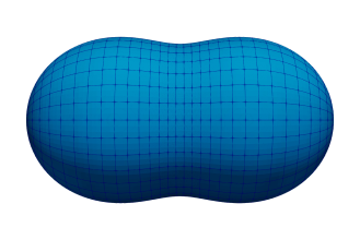
Figure 3: Surface discretization based on quadrilateral elements.

To fix some nomenclature for the following sections, we briefly describe the parameters required to define the discretization (see Figure 3). First, the surface $\Sigma$ is discretized by quadrilateral elements, where the reference element is given by $[-1,1]\times[-1,1]$. On these elements, tensor product Gauss-Legendre nodes and weights of order $P$ are used to provide the quadrature rule for the Nyström method. In-element interpolation is performed using the orthonormal Legendre polynomials of the same order. For the spherical harmonic representation of Section 4.2, we require an equidistant discretization in the $(\theta,\phi)$ charts. For this, we use $M_{\theta}$ and $M_{\phi}$ elements in the $\theta$ and $\phi$ directions, respectively, for a total of $M\triangleq M_{\theta}\times M_{\phi}$ elements. Then, the QBX method requires a local expansion of the kernel up to order $P_{qbx}$. The QBX method, as implemented in pytential, uses an oversampled quadrature grid of order $P_{quad}$ (on top of the base grid of order $P$) to ensure sufficient resolution (see [20] for additional details). Finally, for the FMM, additional expansions (local and multipole) of order $P_{fmm}$ are required.

4.2 Spherical Harmonics and Filtering

We use spherical harmonics to represent the surface and all related geometric quantities, such as the normal and curvature. For a similar application to Stokes flow, see [27], where spherical harmonics were also used to express the layer potentials. The spherical harmonic transforms are performed with the aid of the SHTns [33] open-source library described in [34]. For a smooth closed surface (with a spherical topology) $\Sigma$ and a chosen parametrization $\vect{X}(\theta,\phi):[0,\pi]\times[0,2\pi]\to\Sigma$, we express

$$\vect{X}(\theta,\phi)=\sum_{n=0}^{N_{\theta}}\sum_{m=0}^{\min(n,N_{\phi})}\vect{X}^{m}_{n}Y^{m}_{n}(\theta,\phi),$$

where $Y^{m}_{n}$ are the spherical harmonics of order $m$ and degree $n$. They are given by

$$Y^{m}_{n}(\theta,\phi)\triangleq\sqrt{\frac{2n+1}{4}\frac{(n-m)!}{(n+m)!}}P^{m}_{n}(\cos\theta)e^{\imath m\phi}\quad\text{and}\quad P^{m}_{n}(x)\triangleq(-1)^{m}\frac{(1-x^{2})^{\frac{m}{2}}}{2^{n}n!}\od{{}^{m+n}}{x^{m+n}}(x^{2}-1)^{n},$$

where $P^{m}_{n}(x)$ are the associated Legendre functions of the first kind with the Cordon-Shortley phase included as a matter of convention. The spherical harmonics defined as above form an orthonormal basis for square-integrable functions on the unit sphere $\mathbb{S}^{2}$ when $N_{\theta},N_{\phi}\to\infty$. In practice, we choose

$$N_{\theta}\lesssim\left\lfloor\frac{PM_{\theta}}{2}\right\rfloor\quad\text{and}\quad N_{\phi}\lesssim\left\lfloor\frac{PM_{\phi}}{2}\right\rfloor,$$

as required by the SHTns library. The main difficulty in our discretization arrives when attempting to project between the nodes used by the QBX method and the spherical harmonic coefficients. We perform this projection in three steps, as shown in Figure 4.

Figure 4: Projection to and from the spherical harmonic coefficients and the QBX quadrature grid. (a) Layer 1 represents the spectral coefficients, (b) Layer 2 represents an equidistant grid used by the SHTns [33] library to compute the coefficients, and (c) Layer 3 represents the discontinuous grid of quadrature nodes used by the Nyström-QBX method.

First, the SHTns [33] library uses a uniform grid, for which FFT-type methods are well-suited and provide a substantial speed-up. On the other hand, the Nyström-QBX method described in Section 4.1 is implemented on a Discontinuous Galerkin-type quadrature grid, where continuity between the elements is not enforced. The roundtrip is performed as follows:

• Backward. From the spectral coefficients, we use the SHTns library to obtain the physical values on the equidistant Layer 2 grid. These values are then copied to an equidistant grid where each node is unique. Finally, the values are interpolated element-wise to the Layer 3 quadrature grid using the Legendre polynomials.

• Forward. From the quadrature nodes on the Layer 3 grid, we interpolate back to an equidistant grid on the reference element. Then, to obtain unique values at vertices and faces, the repeated values on the element faces are averaged. Finally, the SHTns library is used to obtain the spectral coefficients.

As we can see, there are several sources of unwanted errors in this construction. First, in both the forward and backward transforms, we have an interpolation from the chosen quadrature grid. This operation is well-conditioned, due to the choice of Gauss-Legendre nodes and the Legendre orthonormal polynomials on the reference element. The main source of error comes from the averaging performed in the forward transform to obtain unique values at the vertices and faces of each element. This operation can introduce spurious high-frequency components into the spectrum and rapidly lead to growing instabilities in the evolution of the droplets. An example of the resulting errors can be seen in Figure 5, where the normal vector was computed on the unit sphere and then projected to its spherical harmonic coefficients. We know that the $x$ component of the normal vector only contains the $Y^{1}_{1}(\theta,\phi)$ mode, but additional modes due to the interpolation and averaging appear in the result.

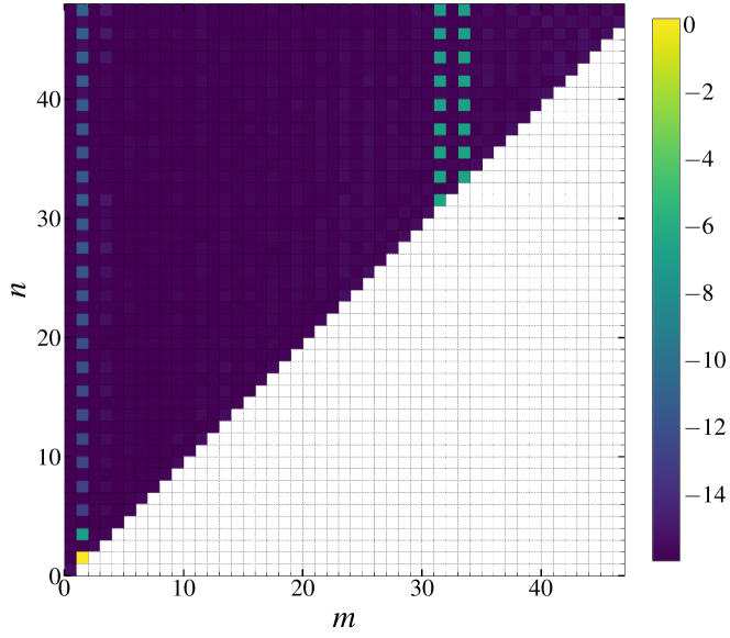
(a)

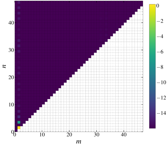
(b)

Figure 5: Filtering: Spherical harmonic coefficients of the $x$ component of the normal vector on a unit sphere. (a) Original projection and (b) filtered projection by (22) with $\alpha=10^{-5}$ and $p=1$. The mesh used $M_{\theta}=M_{\phi}=32$ elements and $P=3$.

In general, we know that the errors introduced by the method must have a frequency that is proportional to the element grid spacing in each direction $(\theta,\phi)$. Therefore, a method that can alleviate these problems would be to simply filter out all modes above a certain wavenumber using a standard ideal filter. This is possible in the $\phi$ direction, where the modes are essentially Fourier modes. However, in the $\theta$ direction, we encounter the associated Legendre functions, where the unique Fourier modes cannot be obtained, and filtering is not as clear. For these reasons, we adopt a hybrid scheme with the filter

$$\hat{F}^{m}_{n}=\begin{cases}\displaystyle\frac{F^{m}_{n}}{1+\alpha(n(n+1))^{2p}},&\quad m<M_{\theta}/2,\\ 0,&\quad\text{otherwise},\end{cases}$$ (22)

where $\alpha\ll 1$ is a real constant and $p\in\mathbb{N}$ is an integer power. We can see here that the orders $m$ are filtered using an ideal filter and the degrees $n$ are weighted in terms of the parameters $\alpha$ and $p$. This weighting is essentially a form of Tikhonov regularization (see [35]) which minimizes

$$\frac{1}{2}\int_{\mathbb{S}^{2}}|f-F|^{2}\dx[S]+\frac{\alpha}{2}\int_{\mathbb{S}^{2}}|\Delta^{p}_{\mathbb{S}^{2}}F|^{2}\dx[S],$$

where $f$ is the function in question an $F$ is its projection to the spherical harmonic basis. The desired expression can then be obtained by using the fact that the spherical harmonics are eigenfunctions of the Laplace-Beltrami operator on the sphere, i.e.

$$\Delta_{\mathbb{S}^{2}}Y^{m}_{n}=-n(n+1)Y^{m}_{n}.$$

In practice, we have found that $p=2$ and $\alpha\approx 10^{-5}$ provides sufficient filtering to stabilize the droplet evolution. These parameters can also be determined directly from the data by, e.g., minimizing a Generalized Cross-Validation functional [36]. The filtered coefficients of the normal of a unit sphere can also be seen in Figure 5.

4.3 Time Stepping and Adaptation

We discretize the evolution equation (1) with the kinematic condition (4) using a second-order explicit method

$$\tilde{\vect{X}}^{n+1}= \vect{X}^{n}+\Delta t^{n}\vect{V}(t^{n},\vect{X}^{n}),$$ (23)

$$\vect{X}^{n+1}= \frac{1}{2}\vect{X}^{n}+\frac{1}{2}\left\{\tilde{\vect{X}}^{n+1}+\Delta t^{n}\vect{V}(t^{n+1},\tilde{\vect{X}}^{n+1})\right\},$$

where both the velocity field and the geometry in the source term are computed at the time $t^{n}$. We have found that higher-order time integration does not offer significant improvement in stability and volume conservation. However, the cost of multiple solutions to (21) can quickly dominate. This is more important in optimization, where we must solve the geometry evolution equation and the normal adjoint transverse field equation a potentially large number of times. For comparison, in [37] (2D), the authors have used an embedded second-order method and in [27] (3D) first-order explicit and implicit schemes have been analyzed. In [18], we have analyzed an axisymmetric formulation coupled with a third-order SSP RK3 time integrator to match the spatial discretization order. The time step is fixed, but proportional to a characteristic mesh size

$$\Delta t=Ch_{max},\quad\text{where }h_{\max}=\max_{i\in\{0,\dots,M\}}\max(\sigma_{i,1},\sigma_{i,2}),$$

where $\sigma_{i}$ are the eigenvalues of the metric tensor at each point $\vect{X}_{i}(0)$. This approximation for a characteristic mesh length is suited for scenarios where the elements can be highly skewed, e.g. at the poles. Improved time step adaptation for long-time simulations can be found, e.g., in [38].

The largest issue when performing the droplet evolution, for medium to long time spans, is the potentially rapid degradation of the mesh. Even for a single droplet in a uniform flow, using the kinematic condition (4) without $\vect{w}$ will cluster the points in the downstream region of the droplet. Therefore, it is necessary to implement a method that either maintains or improves the mesh quality during the evolution. In our implementation, we prefer to make use of so-called “passive” mesh adaptation methods, where a tangential velocity field is added as in (4)

This tangential field is chosen in such a way that, over several iterations, it can improve the quality of the mesh. For two-dimensional flows, the methods presented in [39] are a robust solution that preserves arclength or clusters points in regions of higher curvature. However, in three-dimensional flows, it becomes increasingly difficult to develop robust methods that maintain the mesh quality. We use the tangential velocity field described in [40]. In this method, we find a velocity field that (approximately) minimizes

$$F(\vect{w})=\frac{\alpha}{2}\sum_{ij}\left[\od{}{t}\left(\frac{\|\vect{x}_{ij}\|^{2}}{h_{ij}^{2}}+\frac{h_{ij}^{2}}{\|\vect{x}_{ij}\|^{2}}\right)\right]^{2}+\frac{\beta}{2}\sum_{m}\frac{1}{C_{m}^{2}}\left[\od{C_{m}}{t}\right]^{2},$$ (24)

where $\alpha,\beta\in\mathbb{R}_{+}$. Here, $\vect{x}_{ij}$ denotes the edge between the vertices $(\vect{x}_{i},\vect{x}_{j})$, $h_{ij}$ is a corresponding curvature-based length scale and $C_{m}$ measures the ratio between the element area and its edge lengths. In A, we define the terms in this cost functional and give appropriate extensions to quadrilateral elements (as [38] is focused on simplices). As we will not be stress testing this method with high deformations, we have found it sufficient to ensure the mesh maintains sufficient quality and the simulation remains stable for longer times. A summary of all the steps required to solve the forward problem are given in Algorithm 1.

Data: Number of elements $(M_{\theta},M_{\phi})$; Spherical harmonic expansion orders $(N_{\theta},N_{\phi})$; Gauss-Legendre quadrature order $P$ and $P_{quad}$; QBX order $P_{qbx}$; FMM order $P_{fmm}$.

Data: Final time $T$; time step $\Delta t$ or Courant number $C$.

Data: Initial parametrization $\vect{X}_{0}$ for the surface $\Sigma(0)$.

foreach $n\in\{0,\dots,N-1\}$ do

      

1. Solve for the density $\vect{q}^{n}$ in (21) using the boundary conditions of (2).

2. Compute the velocity field $\vect{u}^{n}$ using (20).

3. Compute the tangential velocity field $\vect{w}^{n}$ solving (24).

4. Checkpoint solutions $(\vect{q}^{n},\vect{X}^{n})$ for the adjoint problem.

5. Evolve interface in time using (23) and apply the filter (22) to the right-hand side at each stage.

Set cost as $J=y^{N}$.

Algorithm 1 Two-phase Stokes Interface Evolution.

As part of the optimization problem, we must also compute the cost (5). This is generally done by noting that

$$J=\int_{0}^{T}j(\vect{u},\vect{X},\vect{g})\dx[t],$$

can also be understood as an ODE. In particular, let

$$\begin{cases}\dot{y}(t)=j(\vect{u},\vect{X},\vect{g}),\\ y(0)=0,\end{cases}$$ (25)

then we have that $J=y(T)$. In the form of an ODE, we can make use of the same time integration method as for the equation themselves and obtain an accurate approximation of time-dependent cost functionals.

4.4 Adjoint Discretization

In the previous sections, the focus has been exclusively on the state equations and the evolution of the droplets. For the adjoint system, we have a similar set of equations to solve. First, we can see from (12) and (13) that the adjoint Stokes equations have the exact same structure as the state equations. Therefore, the same solver can be used in both cases, while only accounting for the differences in boundary conditions. Then, we are left with discretizing the normal adjoint transverse equation from (19). In this case, we simply write

$$-\od{X^{*}}{t}=V^{*}[t,X^{*};\vect{X}],$$

which is discretized with the dual consistent scheme

$$\tilde{X}^{*,n}= X^{*,n+1}+\Delta t^{n+1}V^{*}[t^{n+1},X^{*,n+1};\tilde{\vect{X}}^{n}],$$ (26)

$$X^{*,n}= \frac{1}{2}X^{*,n+1}+\frac{1}{2}\left\{\tilde{X}^{*,n}+\Delta t^{n+1}V^{*}[t^{n},\tilde{X}^{*,n};\vect{X}^{n}]\right\},$$

where the state and adjoint variables are not computed at the same times. We express the terms in right-hand side $V^{*}$ in a strong form through the layer potentials defined in Section 4.1 and all their derivatives. A complete description of the steps is given in Algorithm 2. As in the case of Algorithm 1, an approximation of the gradient can be incorporated if the control is not time-dependent.

Data: Solutions $(\vect{q}^{n},\vect{X}^{n})$ of the forward problem for all $n$.

foreach $n\in\{N-1,\dots,1\}$ do

      

1. Solve for the density $\vect{q}^{*,n+1}$ in (21) using the boundary conditions of the adjoint problem (12).

2. Compute the adjoint velocity field $\vect{u}^{*,n+1}$ using (20).

3. Evolve the normal adjoint transverse field using (26) by applying the filter (22) to the right-hand side at each stage.

4. If the control is time dependent, then use (27) to update the components at time $t^{n}$. Otherwise, evolve an ODE similar to (25) to accumulate the final gradient.

Algorithm 2 Normal Adjoint Transverse Field Evolution.

When using a discretize-then-optimize approach to adjoint optimization, the forward and adjoint problems have exactly the same time step requirements (as the operators in question are just Hermitian transposes of each other). However, for an optimize-then-discretize approach this is no longer the case and additional errors can appear due to a lack of dual consistency. We have not found this to be an issue in our simulations, so the same time step is used.

4.5 Gradient Descent

The optimization problem (6) can now be solved by standard gradient descent methods. In particular, we can use Algorithm 1 and Algorithm 2 as black boxes used to compute the cost functional values and the corresponding gradient at every $\vect{g}^{(k)}$. Then, a steepest descent update is applied

$$\vect{g}^{(k+1)}=\vect{g}^{(k)}+\alpha^{(k)}\nabla_{\vect{g}}J(\vect{g}^{(k)}),$$ (27)

where $\alpha^{(k)}$ is a chosen step size. In this work, we use the Barzilai-Borwein method from [41] to approximate a value for $\alpha^{(k)}$ at every step of the optimization. If this value does not result in a decrease of the cost functional, we set $\alpha^{(k)}\leftarrow\alpha^{(k)}/2$ until a decrease is achieved. This approximation was chosen to avoid a more complicated line search, as evaluating the cost functional through Algorithm 1 can be very costly. The complete method is described in Algorithm 3.

Data: Initial guess $\vect{g}^{(0)}$ for the control.

Data: Tolerances for the cost functional values $\epsilon_{J}$, the gradient $\epsilon_{\nabla}$ and the step size $\alpha_{max}$.

foreach $k\in{0,\dots,K}$ do

      

1. Compute the cost functional $J(\vect{g}^{(k)})$ using Algorithm 1.

2. Compute the gradient $\nabla_{\vect{g}}J(\vect{g}^{(k)})$ using Algorithm 2.

3. Estimate $\alpha^{(k)}$ using the Barzilai-Borwein method bounded by $\alpha_{max}$.

4. Update the control

   $$\vect{g}^{(k+1)}=\vect{g}^{(k)}+\alpha^{(k)}\nabla_{\vect{g}}J(\vect{g}^{(k)}),$$

5. If $J(\vect{g}^{(k+1)})>J(\vect{g}^{(k)})$, attempt the update again with $\alpha^{(k)}/2$.

6. Check stopping criteria

   $$|J(\vect{g}^{(k+1)})|<\epsilon_{J}\quad\text{or}\quad\|\nabla_{\vect{g}}J(\vect{g}^{(k+1)})\|<\epsilon_{\nabla}.$$

Algorithm 3 Adjoint-based Optimization of Quasi-static Two-Phase Stokes Flow.

5 Numerical Results

We present several static and quasi-static test cases to serve as verification for the adjoint-based optimal control of two-phase Stokes flows presented in the previous sections. For simplicity, we fix a set of discretization parameters in Table 1. The number of elements and spherical harmonic orders will be case-dependent.

Parameter	Description	Value
$P$	Base quadrature rule order	3
$P_{quad}$	Oversampled quadrature rule order	$4P$
$P_{qbx}$	QBX expansion order	4
$P_{fmm}$	FMM expansion order	10

Table 1: Default discretization parameters used in Test 1-3

5.1 Test 1: Verification of the Adjoint Gradient

As a first test, we will present some results to verify the adjoint equations presented in Section 2. The standard method to verify a continuous adjoint in the optimize-then-discretize setting is by comparing the gradient to a black-box finite different approximation. For our work, it is very difficult to obtain clear convergence results, due in part to the moving geometry and the complexity of the source terms in the adjoint transverse field equation (8). Therefore, in this test we remove the moving geometry and focus on verifying the right-hand side source terms. As shown in [18], these terms are essentially part of the shape gradient of the static problem. In our cost functional (5), we take

$$J\triangleq\frac{1}{2}\int_{\Sigma}(\vect{u}\cdot\vect{n})^{2}\dx[S],$$

i.e. $\alpha_{1}=1,\alpha_{2}=\alpha_{3}=0$ and $u_{d}=0$. To compute a finite difference approximation of the shape gradient, we use

$$g_{FD,i}\triangleq\inp{\vect{g},\vect{h}_{i}}_{\Sigma}\approx\frac{J(\vect{X}+\epsilon\vect{h}_{i})-J(\vect{X})}{\epsilon},$$ (28)

where $\vect{g}$ is the gradient and $\vect{h}_{i}\triangleq h_{i}\vect{n}$ is a chosen bump function. Typically in finite different approximations, $h_{i}$ is chosen to be a Dirac Delta point mass, but this is not possible here as we require a smooth perturbation of the geometry $\vect{X}$. We use

$$h_{i}(\vect{X})=\frac{1}{\sqrt{2\pi}\sigma}\exp\left(-\frac{\|\vect{X}-\vect{X}_{i}\|}{2\sigma^{2}}\right),$$

where the standard deviation $\sigma$ is taken to be $10^{-1}$. In general, a good choice of $\sigma$ depends on the mesh spacing. As the bump functions are not given pointwise, to compare the finite different approximation with the adjoint-based approximation, we must also convolve the adjoint based gradient

$$g_{AD,i}\triangleq\inp{\nabla_{\vect{X}}J,\vect{h}_{i}}_{\Sigma},$$

where the inner product is computed using the quadrature rules of the Nyström-QBX method from Section 4.1. The errors are given by

$$E[\vect{g}_{AD},\vect{g}_{FD}]\triangleq\frac{\|\vect{g}_{AD}-\vect{g}_{FD}\|_{2}}{\|\vect{g}_{FD}\|_{2}},$$

in the standard square-summable $\ell^{2}$ norm. It would be prohibitively expensive to compute a perturbation for the finite difference approximation at all the points in the geometry, especially on finer meshes. We have chosen here $5$ random points on a sphere of radius $R=1$ at which to compute the finite difference gradient and the errors.

$\epsilon$	$(\lambda=1,\mathrm{Ca}=1)$	EOC	$(\lambda=10,\mathrm{Ca}=\infty)$	EOC
1.00e-01	3.886568e-02	—	1.221459e-01	—
1.00e-02	4.032369e-03	0.98	1.348132e-02	0.96
1.00e-03	6.707820e-04	0.78	1.747667e-03	0.89
1.00e-04	5.016154e-04	0.13	6.727348e-04	0.41
1.00e-05	4.956386e-04	0.01	5.883712e-04	0.06

Table 2: Test 1: Relative errors for the finite difference vs adjoint gradient approximations for $(\lambda,\mathrm{Ca})$ as $(1,1)$ and $(10,\infty)$.

For the discretization, we have chosen a sufficiently fine grid to showcase the first-order convergence of the finite difference approximation (28). In general, we expect that the error has two parts $\mathcal{O}(\epsilon)+\mathcal{O}(h_{max}^{P})$. For this experiment, as we vary $\epsilon$, we expect to see first-order convergence until a plateau determined by the discretization error that depends on $h_{max}$. In [18], we have shown convergence with respect to the mesh spacing as well. The discretization in this case is formed out of $M_{\theta}=M_{\phi}=64$ elements and $N_{\theta}=N_{\phi}=94$ spherical harmonic coefficients. No additional filtering is performed on the gradient. For the two-phase Stokes problem, we have used $\lambda=1$ and $\mathrm{Ca}=1$ as base parameters. Then, the farfield boundary conditions are given by

$$\vect{u}_{\infty}=(\alpha x,-2\alpha y,\alpha z)\quad\text{and}\quad p_{\infty}\equiv 0,$$ (29)

i.e. an extensional flow along the $y$ axis. This choice was made to match the axisymmetric extensional flow used in [18]. The resulting relative errors can be seen in Table 2. The first-order convergence is recovered for both $\mathcal{S}^{*}$ and $\mathcal{C}^{*}$ terms in the adjoint-based gradient (see (14)). For completeness, the pointwise errors can be seen in Figure 6 at the chosen points

$$(m,p)\in\{(3652,2),(3574,9),(2723,7),(1614,3),(322,1)\},$$

where $m$ denotes the element and $p$ denotes the local node index inside the element.

data_convergence_capillary_errors

(a)

data_convergence_viscosity_errors

(b)

Figure 6: Test 1: Absolute errors for the finite difference vs adjoint gradient approximations for $(\lambda,\mathrm{Ca})$ as $(1,1)$ and $(10,\infty)$.

5.2 Test 2: Steady State Tracking

Next, we will look at a simple shape optimization problem using the gradient that we have verified in the previous section. The problem involves finding a steady state of the Stokes flow in a particular configuration. The setup we will be following is presented in [42], where a single droplet has been suspended in an axisymmetric extensional flow. We will attempt to find the steady state for $(\lambda=1,\mathrm{Ca}=0.05)$ in the extensional flow (29) and match the results from [42]. The cost functional we will be using is

$$J=\frac{1}{2}\int_{\Sigma}(\vect{u}\cdot\vect{n})^{2}\dx[S]+\frac{1}{2}(V-V_{d}),$$ (30)

where the volumes

$$V_{d}\triangleq\frac{4\pi}{3}R^{3}\quad\text{and}\quad V\triangleq\int_{\Omega_{-}}\dx[S]=\frac{1}{d}\int_{\Sigma}\vect{x}\cdot\vect{n}\dx[S]$$

are used to enforce volume conservation in the optimization problem. Note that, unlike the kinematic condition 4, the shape optimization problem will not attempt to keep a constant volume. The discretization from section 5.1 is used.

With this setup in mind, we perform two separate optimization problems to gauge the benefit of using the full power of shape optimization on the cost functional from (30). First, we start by finding an optimal spheroid that matches our volume and minimizes the normal velocity $\vect{u}\cdot\vect{n}$. This problem has been studied in [40], where an analytical solution is found on a prolate spheroid. This analytical solution is then used as part of an optimization problem to determine the parametrization of the spheroid that minimizes $\vect{u}\cdot\vect{n}$, in the same way that we are attempting to do here. In [40], the authors perform this optimization for a wide range of $(\lambda,\mathrm{Ca})$ and compare the results to existing literature. We will restrict ourselves to the single case with $\lambda=1$ and $\mathrm{Ca}=0.05$. Before we can continue, we detail the parametrization of the spheroid and how the adjoint-based gradient can be computed with respect to the new parameters. First, we have that the spheroid is given by

$$\vect{S}(\theta,\phi;R,a,\alpha,\beta,\gamma)\triangleq\vect{R}(\alpha,\beta,\gamma)\begin{bmatrix}R\sin\theta\cos\phi\\ R\sin\theta\sin\phi\\ aR\cos\theta,\end{bmatrix}$$

where $R$ is the radius and $a$ is the aspect ratio of the spheroid. The rotation matrix is given in terms of the Euler angles as

$$\vect{R}(\alpha,\beta,\gamma)=\vect{R}_{z}(\alpha)\vect{R}_{y}(\beta)\vect{R}_{x}(\gamma),$$

where each $\vect{R}_{i}$ matrix rotates around the $i$ axis. Then, we use the parameters $\vect{s}\triangleq(R,a,\alpha,\beta,\gamma)\in\mathbb{R}_{+}^{2}\times\mathbb{R}^{3}$ as our control variables and strive to find the gradient of the cost functional from (30) with respect to $\vect{s}$ instead of $\vect{X}$. The gradient is obtained by a straightforward application of the chain rule as

$$\pd{J}{s_{i}}=\int_{\Sigma}\nabla_{\vect{X}}J\vect{n}\cdot\pd{\vect{S}}{s_{i}}\dx[S],$$

where

$$\pd{\vect{S}}{R}=\frac{1}{R}\vect{S},\qquad\pd{\vect{S}}{a}=\vect{R}(\alpha,\beta,\gamma)\begin{bmatrix}0&0&0\\ 0&0&0\\ 0&0&1/a\end{bmatrix}\vect{R}^{T}(\alpha,\beta,\gamma)\mathbf{S},$$

and the derivative with respect to the Euler angle $\alpha$ is given by (similarly for $\beta,\gamma$)

$$\pd{\vect{S}}{\alpha}=\pd{\vect{R}}{\alpha}\vect{R}^{T}\vect{S},\quad\text{where }\quad\pd{\vect{R}}{\alpha}=\od{\vect{R}_{z}}{\alpha}\vect{R}_{y}(\beta)\vect{R}_{x}(\gamma)=\begin{bmatrix}-\sin\alpha&-\cos\alpha&0\\ \cos\alpha&-\cos\alpha&0\\ 0&0&0\end{bmatrix}\vect{R}_{y}(\beta)\vect{R}_{x}(\gamma).$$

The gradient described above is not the complete gradient with respect to $\vect{s}$ that we expect. The discrepancy comes from the fact that, in obtaining the shape gradient, we have assumed that the perturbations $\tilde{\vect{V}}$ only have a normal component (see (7)). However, for this problem, the perturbations are actually given by

$$\tilde{\vect{V}}\triangleq\od{\vect{S}}{s_{i}},$$

which have tangential components.

optim_qbx_shape_spheroid_cost

(a)

optim_qbx_shape_spheroid_gradient

(b)

Figure 7: Test 2: (a) Cost functional and (b) Gradient $\ell^{2}$ norm for the spheroid optimization, normalized with respect to initial guess.

For the optimization parameters, we start with a sphere of radius $R=1$, much like we would start the genuine evolution equation (1) in an attempt to find the steady state. Therefore, for the spheroid parameters, we take $\vect{s}^{(0)}\triangleq(1,1,0,0,0)$, while the full shape optimization will use $\vect{X}^{(0)}\triangleq\vect{S}(\theta,\phi;\vect{s}^{(0)})$. We have performed optimizations with non-zero angles $(\alpha,\beta,\gamma)$ and observed similar results, but for the sake of comparison, we reduce here to this simple case.

optim_qbx_shape_3d_cost

(a)

optim_qbx_shape_3d_gradient

(b)

Figure 8: Test 2: (a) Cost functional and (b) Gradient $\ell^{2}$ norm for the shape optimization, normalized with respect to initial guess.

The results for the spheroid optimization are provided in Figure 7. We can see that the cost functional plateaus at $J\approx 10^{-4}$, while the gradient is about two orders of magnitude smaller. This indicates that we have indeed found a minimum for this optimization problem, even if it is not $J\approx 0$. A clear benefit of this choice is that the optimization only required $36$ steps to achieve convergence and find a shape with $\|\vect{u}\cdot\vect{n}\|_{2}\approx 10^{-2}$. In many situations of interest this is a sufficiently accurate result.

In the spheroid optimization, the cost functional cannot reach the minimum solution as the steady state of a droplet in extensional flow is not exactly a spheroid. Therefore, as a second experiment, we attempt to perform a full shape optimization and see if better convergence can be obtained. This is indeed the case, as shown in Figure 8. Here, the cost functional reached a minimum value of $10^{-6}$, two orders of magnitude smaller than in the spheroid case. Therefore, if we want to find a true steady state shape to arbitrary precision, the full shape optimization problem is required. The downside, however, is that the optimization required roughly $400$ steps to reach the minimum, making it significantly more costly, i.e. $13\times$ for an increase in accuracy of two orders of magnitude. This is more in line with the requirements of computing the steady state using (4).

optim_qbx_shape_spheroid_volume

(a)

optim_qbx_shape_spheroid_deformation

(b)

Figure 9: Test 2: (a) Droplet volume $|\Omega_{-}|$ and (b) deformation during the optimization for the spheroid (full) and shape (dashed) optimization.

To see if the optimization reached the expected steady state shape, we briefly investigate the volume and deformation during the optimization for both cases. First, we can see the improved behavior in the convergence of the volume and deformation of the droplet in Figure 9. Following [42], the deformation is defined simply as

$$D\triangleq\frac{L-H}{L+H},$$

where $L$ is the half-length and $H$ is the half-height of the droplet in the $x$-$z$ plane. An approximation of the results obtained in [42] is also provided (the exact values are not available). While it is hard to determine an improvement in the deformation, we can clearly see that the volume is not accurately conserved when performing the spheroid optimization, as there is a noticeable gap in Figure 9a. This is due to the fact that the velocity term in the cost functional is dominating and did not allow convergence of the smaller volume term.

5.3 Test 3: Unsteady Helix

Figure 10: Test 3: Helical trajectory of a particle.

For a quasi-static optimization problem, we attempt to match the movement of two droplets against a desired helical trajectory. The cost functional we will be using is given by

$$J=\frac{1}{2}\sum_{i\in\{+,-\}}\int_{0}^{T}\int_{\Sigma_{i}}\|\vect{x}_{c,i}(t)-\vect{x}_{c,d,i}(t)\|^{2}\dx[S]\dx[t],$$

where $\vect{x}_{c,\pm}$ are the centroids of the two droplets. The desired centroids are taken as the centroids of two spheres of radius $R$, i.e.

$$\vect{x}_{c,d,\pm}(t;\omega_{d},H_{d})=\begin{bmatrix}\cos\omega_{d}t/T&-\sin\omega_{d}t/T&0\\ \sin\omega_{d}t/T&\cos\omega_{d}t/T&0\\ 0&0&1\end{bmatrix}\begin{bmatrix}\pm 2R\\ 0\\ 0\end{bmatrix}+\begin{bmatrix}0\\ 0\\ H_{d}t/T\end{bmatrix},$$ (31)

in the time interval $t\in[0,T]$, where $\omega_{d},H_{d}\in\mathbb{R}_{+}$ denote the wavenumber and the height of the helix, respectively. The initial conditions $\vect{X}_{0,\pm}(\theta,\phi)$ are also taken to be spheres of radius $R=1$. The velocity field that gives rise to the trajectory from (31) is essentially a solid body rotation in the $x$-$y$ plane and a uniform flow along the $z$ axis. We will use a parametrization in terms of $(\omega,H)$ of the farfield as our control variables. As such, the farfield boundary conditions are given by

$$\vect{u}_{\infty}(t,\vect{x};\omega,H)\triangleq-\frac{\omega}{T}y\vect{e}_{x}+\frac{\omega}{T}x\vect{e}_{y}+\frac{H}{T}\vect{e}_{z}\quad\text{and}\quad p_{\infty}(t,\vect{x};\omega,H)\equiv 0,$$

which will result in a classical helical trajectory seen in Figure 10. To complete the definition of the two-phase Stokes problem, we again choose $\lambda=1$ and $\mathrm{Ca}=0.05$. In this case, the adjoint-based gradient is given by

$$\pd{J}{\omega}= \frac{1}{T}\int_{0}^{T}\int_{\Sigma(t)}(\vect{X}^{*}\cdot\vect{n})(xn_{y}-yn_{x})\dx[S]\dx[t],$$

$$\pd{J}{H}= \frac{1}{T}\int_{0}^{T}\int_{\Sigma(t)}(\vect{X}^{*}\cdot\vect{n})n_{z}\dx[S]\dx[t].$$

optim_qbx_helix_cost

(a)

optim_qbx_helix_gradient

(b)

Figure 11: Test 3: Normalized (a) cost functional values and (b) gradient norm values.

The spatial discretization of the droplets is similar to that of the previous example. We set $M_{\theta}=M_{\phi}=24$ elements and $N_{\theta}=N_{\phi}=45$ spherical harmonic coefficients. As mentioned in Section 4.3 and Section 4.4, we apply a filter at every step of the evolution, both for the forward and the adjoint calculations. The droplets are evolved using the second-order SSP RK time integrator to a final time of $T=\pi$ with a fixed time step of $\Delta t=10^{-2}$. The time step was chosen to ensure stability during the evolution of the geometry using the desired control $(\omega_{d},H_{d})$. We make use of the tangential forcing from Section 4.3 to ensure the mesh does not significantly degrade during the simulation.

For the optimization, we have chosen to start with $(\omega^{(0)},H^{(0)})=(3\pi,1.5)$ and $(\omega_{d},H_{d})=(4\pi,2)$. The results of the optimization can be seen in Figure 11. We can see that both the cost functional and the gradient are significantly decreased during the optimization process. In particular, the gradient has decreased by about three orders of magnitude and the cost has decreased by about five orders of magnitude. The convergence of both quantities is well-behaved throughout the optimization, when considering the naive line search algorithm used. To better understand the convergence to the optimal solution, we turn to Figure 12. We can see here that both the parameters $(\omega,H)$ approach their respective desired values in only a few iterations. Comparing to Figure 11, we can see that once the wavenumber $\omega$ becomes close to $\omega_{d}$, the optimization changes its behavior and the error decreases linearly.

optim_qbx_helix_control

(a)

optim_qbx_helix_centroid_x

(b)

Figure 12: Test 3: (a) Convergence of the control variables $(\omega,H)$ to their desired values (dashed). (b) Centroid $\vect{x}_{c}(t)$ (dashed gray) for the droplet starting at $(-R,0,0)$ and the desired centroid trajectory (dashed orange).

6 Conclusions

We have developed a methodology for applying optimal control to the Stokes flow of two-phase immiscible fluids with sharp interfaces. We have considered systems with constant surface tension, but extensions to other context can be easily derived (e.g. variable surface tension, gravity, electrostatic). The focus has been on extending the existing results from [18] to fully three-dimensional problems containing multiple interacting droplets.

At the theoretical level, the main contribution of this work has been in deriving a scalar evolution equation for the adjoint transverse field. This is important for the three-dimensional extension, as it provides a non-trivial computational cost reduction. Furthermore, the optimal control theory in the context of moving domains is a very active area of research and the application to two-phase Stokes flow is an important stepping stone to more complex scenarios. However, many open questions remain regarding the general well-posedness of the sensitivity and adjoint equations. Unlike results such as [15], the adjoint transverse field (14) does not satisfy a parabolic-type equation, so much less can be said about its regularity.

We have also presented a numerical scheme based on existing, well-tested libraries that provides sufficient efficiency and robustness to perform optimal control of the two-phase flows. Previous work in [18] has relied on special treatment of each type of singularity and kernel in the adjoint equations, which was mainly possible due to the one-dimensional interface (under axisymmetric assumptions). Extending and developing similar methods for the three-dimensional case is impractical, so we have used the kernel-independent QBX method as an alternative way of handling the many singularities in the boundary integral equations.

The applications presented here have been focused on small deformations of the interface for moderate time horizons. Testing the numerical scheme on longer time spans and large deformations is the subject of further investigation. However, this opens up many additional complexities. For example, issues regarding the general “reachability” of some desired state of the system become important. In this work, we have used controls in $\mathbb{R}^{2}$ for the quasi-static case, but for full control of the system a time- and space-dependent control is likely necessary. Furthermore, we expect the gradient descent to perform increasingly worse as the interface deforms more due to the high nonlinearity of the problem. These issues are common to all shape-based gradient flows and are of great practical and theoretical interest for future research.

Acknowledgements

This work was sponsored, in part, by the Office of Naval Research (ONR) as part of the Multidisciplinary University Research Initiatives (MURI) Program, under Grant Number N00014-16-1-2617.

Declaration of Interests

The authors report no conflict of interest.

Appendix A Mesh Adaptation Functional and Gradient

In this appendix we detail the gradient of the passive mesh stabilization functional from Section 4.3, as originally given in [38]. We start by stating that motion law is $\dot{\vect{x}}=\vect{V}$, where the source term is arbitrary. We must then find a $\vect{V}$ that minimizes

$$J(\vect{V})=\frac{\alpha}{2}\sum_{i}\sum_{j\in\mathcal{N}(i)}\left[\od{}{t}\left(\frac{r_{ij}^{2}}{h_{ij}^{2}}+\frac{h_{ij}^{2}}{r_{ij}^{2}}\right)\right]^{2}+\frac{\beta}{2}\sum_{m}\frac{1}{C_{m}^{2}}\left[\od{C_{m}}{t}\right]^{2},$$

where we will be assuming that $h_{ij}$ does not depend on the choice of $\vect{V}$. We start by looking at the first term, for which we have that

$$r_{ij}^{2}=\|\vect{x}_{i}-\vect{x}_{j}\|^{2},$$

so

$$\frac{1}{2}\od{}{t}\left(\frac{r_{ij}^{2}}{h_{ij}^{2}}+\frac{h_{ij}^{2}}{r_{ij}^{2}}\right)= \frac{1}{h_{ij}^{2}}(\vect{x}_{i}-\vect{x}_{j})\cdot(\vect{V}_{i}-\vect{V}_{j})-\frac{h_{ij}^{2}}{r_{ij}^{4}}(\vect{x}_{i}-\vect{x}_{j})\cdot(\vect{V}_{i}-\vect{V}_{j})$$

$$= \left(\frac{1}{h_{ij}^{2}}-\frac{h_{ij}^{2}}{r_{ij}^{4}}\right)(\vect{x}_{i}-\vect{x}_{j})\cdot(\vect{V}_{i}-\vect{V}_{j}).$$

Figure 13: Numbering of quadrilateral vertices and division intro triangles.

Then, for the compactness factor $C_{m}$, we have that

$$C_{m}=\frac{|\Sigma_{m}|}{\sum_{i=0}^{2^{d}}|\partial\Sigma_{m,i}|^{2}},$$

where $|\Sigma_{m}|$ denotes the area of the element $\Sigma_{m}$ and $|\partial\Sigma_{m,i}|$ are the lengths of its faces. In the case of a quadrilateral element (for surfaces), the formula reduces to (see Figure 13 for notation)

$$C_{m}=\frac{|T_{ABC}|+|T_{BDC}|}{r_{AB}^{2}+r_{BD}^{2}+r_{DC}^{2}+r_{CA}^{2}}.$$

where $|T_{\cdots}|$ denotes the area of the triangle. We can further express the area of the triangles through Heron’s formula as

$$|T_{ABC}|= \frac{1}{4}\sqrt{(r_{AB}^{2}+r_{BC}^{2}+r_{CA}^{2})^{2}-2(r_{AB}^{4}+r_{BC}^{4}+r_{CA}^{4})}=\frac{1}{4}\sqrt{a_{ABC}^{2}-2b_{ABC}},$$

$$|T_{BDC}|= \frac{1}{4}\sqrt{(r_{BD}^{2}+r_{DC}^{2}+r_{BC}^{2})^{2}-2(r_{BD}^{4}+r_{DC}^{4}+r_{BC}^{4})}=\frac{1}{4}\sqrt{a_{BDC}^{2}-2b_{BDC}},$$

so we can write

$$C_{m}=\frac{\sqrt{a^{2}_{ABC}-2b_{ABC}}+\sqrt{a^{2}_{BDC}-2b_{BDC}}}{4(r_{AB}^{2}+r_{BD}^{2}+r_{DC}^{2}+r_{CA}^{2})},$$

where only squares of the edge lengths appear. We now have the simple derivatives

$$\pd{a^{2}_{ABC}}{r_{AB}^{2}}=2(r_{AB}^{2}+r_{BC}^{2}+r_{CA}^{2})=2a_{ABC}\quad\text{and}\quad\pd{b_{ABC}}{r_{AB}^{2}}=2r_{AB}^{2},$$

with equivalent results for derivatives with respect to $r_{BD}^{2},r_{DC}^{2}$ and $r_{BC}^{2}$. Note that $r_{BC}^{2}$ appears in both terms in the numerator, while it does not appear in the denominator. We can now take the derivative to the squared variables $r^{2}_{\cdot\cdot}$ by a simple application of the chain rule. We take $r_{AB}^{2}$ and $r_{BC}^{2}$ as a representative examples, for which we have

$$\od{C_{m}}{r_{AB}^{2}}= \frac{1}{4(r_{AB}^{2}+r_{BD}^{2}+r_{DC}^{2}+r_{CA}^{2})}\left\{\frac{r_{BC}^{2}+r_{CA}^{2}-r_{AB}^{2}}{|T_{ABC}|}-4C_{m}\right\},$$

$$\od{C_{m}}{r_{BC}^{2}}= \frac{1}{4(r_{AB}^{2}+r_{BD}^{2}+r_{DC}^{2}+r_{CA}^{2})}\left\{\frac{r_{AB}^{2}+r_{CA}^{2}-r_{BC}^{2}}{|T_{ABC}|}+\frac{r_{BD}^{2}+r_{DC}^{2}-r_{BC}^{2}}{|T_{BDC}|}\right\}.$$

Finally, the time derivative can be written by the chain rule as

$$\pd{C_{m}}{t}= \pd{C_{m}}{r_{AB}^{2}}\pd{r_{AB}^{2}}{t}+\pd{C_{m}}{r_{BD}^{2}}\pd{r_{BD}^{2}}{t}+\pd{C_{m}}{r_{DC}^{2}}\pd{r_{DC}^{2}}{t}+\pd{C_{m}}{r_{CA}^{2}}\pd{r_{CA}^{2}}{t}+\pd{C_{m}}{r_{BC}^{2}}\pd{r_{BC}^{2}}{t},$$

where

$$\frac{1}{2}\pd{r^{2}_{AB}}{t}=(\vect{x}_{A}-\vect{x}_{B})\cdot(\vect{V}_{A}-\vect{V}_{B}).$$

We now have all the terms of interest and their derivatives. Determining the exact formula for the full gradient is straightforward, as all the terms are simply quadratic in $\vect{V}_{i}$.

References

- [1] C. Pozrikidis, Interfacial dynamics for Stokes flow, Journal of Computational Physics 169 (2) (2001) 250–301. doi:10.1006/jcph.2000.6582.
- [2] G. Huisken, Flow by mean curvature of convex surfaces into spheres, Journal of Differential Geometry 20 (1984) 237–266. doi:10.4310/jdg/1214438998.
- [3] K. Deckelnick, G. Dziuk, C. M. Elliott, Computation of geometric partial differential equations and mean curvature flow, Acta Numerica 14 (2005) 139–232. doi:10.1017/s0962492904000224.
- [4] A. Jameson, Aerodynamic design via control theory, Journal of scientific computing 3 (3) (1988) 233–260.
- [5] M. Hintermüller, D. Wegner, Optimal control of a semidiscrete Cahn–Hilliard–Navier–Stokes system, SIAM Journal on Control and Optimization 52 (2014) 747–772. doi:10.1137/120865628.
- [6] H. Garcke, M. Hinze, C. Kahle, Optimal control of time-discrete two-phase flow driven by a diffuse-interface model, ESAIM: Control, Optimisation and Calculus of Variations 25 (2019) 13. doi:10.1051/cocv/2018006.
- [7] Y. Deng, Z. Liu, Y. Wu, Topology optimization of capillary, two-phase flow problems, Communications in Computational Physics 22 (2017) 1413–1438. doi:10.4208/cicp.oa-2017-0003.
- [8] A. Prosperetti, G. Tryggvason, Computational methods for multiphase flow, Cambridge University Press, 2009.
- [9] S. Popinet, An accurate adaptive solver for surface-tension-driven interfacial flows, Journal of Computational Physics 228 (16) (2009) 5838–5866.
- [10] F. Feppon, G. Allaire, F. Bordeu, J. Cortial, C. Dapogny, Shape optimization of a coupled thermal fluid-structure problem in a level set mesh evolution framework, SeMA Journal 76 (3) (2019) 413–458.
- [11] M. K. Bernauer, R. Herzog, Optimal control of the classical two-phase Stefan problem in level set formulation, SIAM Journal on Scientific Computing 33 (1) (2011) 342–363.
- [12] S. Repke, N. Marheineke, R. Pinnau, Two adjoint-based optimization approaches for a free surface Stokes flow, SIAM Journal on Applied Mathematics 71 (6) (2011) 2168–2184.
- [13] F. Palacios, J. J. Alonso, A. Jameson, Shape sensitivity of free-surface interfaces using a level set methodology, in: 42nd AIAA Fluid Dynamics Conference and Exhibit, 2012.
- [14] A. Laurain, S. W. Walker, Droplet footprint control, SIAM Journal on Control and Optimization 53 (2015) 771–799. doi:10.1137/140979721.
- [15] A. Laurain, S. W. Walker, Optimal control of volume-preserving mean curvature flow, Journal of Computational Physics 438 (2021) 110373. doi:10.1016/j.jcp.2021.110373.
- [16] E. Diehl, J. Haubner, M. Ulbrich, S. Ulbrich, Differentiability results and sensitivity calculation for optimal control of incompressible two-phase Navier–Stokes equations with surface tension (2020). arXiv:2003.04971v1.
- [17] N. Kühl, J. Kröger, M. Siebenborn, M. Hinze, Rung, Adjoint complement to the Volume-of-Fluid method for immiscible flows, Journal of Computational Physics 440 (2021) 110411. arXiv:2009.03957v1, doi:10.1016/j.jcp.2021.110411.
- [18] A. Fikl, D. J. Bodony, Adjoint-based interfacial control of viscous drops, Journal of Fluid Mechanics 911 (2021). doi:10.1017/jfm.2020.1013.
- [19] A. Klockner, A. Barnett, L. Greengard, M. O’Neil, Quadrature by Expansion: A new method for the evaluation of layer potentials, J. Comput. Phys. 252 (2013) 332–349. doi:10.1016/j.jcp.2013.06.027.
- [20] M. Wala, A. Klöckner, A fast algorithm for Quadrature by Expansion in three dimensions, Journal of Computational Physics 388 (2019) 655–689. doi:10.1016/j.jcp.2019.03.024.
- [21] M. Moubachir, J.-P. Zolésio, Moving Shape Analysis and Control: Applications to Fluid Structure Interactions, Chapman and Hall, 2006.
- [22] D. Luft, V. Schulz, Pre-shape calculus: Foundations and application to mesh quality optimization (2020). arXiv:2012.09124v1.
- [23] S. W. Walker, The Shape of Things: A Practical Guide to Differential Geometry and the Shape Derivative, SIAM, 2015.
- [24] G. Allaire, M. Schoenauer, Conception optimale de structures, Springer, 2007.
- [25] O. Pantz, Sensibilité de l’équation de la chaleur aux sauts de conductivité, Comptes Rendus Mathématique 341 (5) (2005) 333–337.
- [26] M. D. Gunzburger, Perspectives in Flow Control and Optimization, SIAM, 2003.
- [27] S. K. Veerapaneni, A. Rahimian, G. Biros, D. Zorin, A fast algorithm for simulating vesicle flows in three dimensions, Journal of Computational Physics 230 (2011) 5610–5634. doi:10.1016/j.jcp.2011.03.045.
- [28] C. Pozrikidis, Boundary Integral and Singularity Methods for Linearized Viscous Flow, Cambridge University Press, 1992.
- [29] A. Fikl, D. J. Bodony, Jump relations of certain hypersingular Stokes kernels on regular surfaces, SIAM Journal on Applied Mathematics 80 (2020) 2226–2248. doi:10.1137/19m1269804.
- [30] R. Kress, Linear Integral Equations, Springer, 1989.
- [31] A. Klockner, Collaborators, pytential https://github.com/inducer/pytential (2021).
- [32] A. T. Tornberg, L. Greengard, A fast multipole method for the three-dimensional Stokes equations, J. Comput. Phys. 227 (3) (2008) 1613–1619. doi:10.1016/j.jcp.2007.06.029.
- [33] N. Schaeffer, SHTns https://bitbucket.org/nschaeff/shtns (2021).
- [34] N. Schaeffer, Efficient spherical harmonic transforms aimed at pseudospectral numerical simulations, Geochemistry, Geophysics, Geosystems 14 (2013) 751–758. doi:10.1002/ggge.20071.
- [35] R. G. McClarren, C. D. Hauck, Robust and accurate filtered spherical harmonics expansions for radiative transfer, Journal of Computational Physics 229 (2010) 5597–5614. doi:10.1016/j.jcp.2010.03.043.
- [36] G. H. Golub, M. Heath, G. Wahba, Generalized cross-validation as a method for choosing a good ridge parameter, Technometrics 21 (1979) 215–223. doi:10.1080/00401706.1979.10489751.
- [37] R. Ojala, A. T. Tornberg, An accurate integral equation method for simulating multi-phase Stokes flows, J. Comput. Phys. 298 (2015). doi:10.1016/j.jcp.2015.06.002.
- [38] A. Z. Zinchenko, R. H. Davis, Emulsion flow through a packed bed with multiple drop breakup, Journal of Fluid Mechanics 725 (2013) 611–663. doi:10.1017/jfm.2013.197.
- [39] M. C. A. Kropinski, An efficient numerical method for studying interfacial motion in two-dimensional creeping flows, Journal of Computational Physics 171 (2001) 479–508. doi:10.1006/jcph.2001.6787.
- [40] M. Zabarankin, I. Smagin, O. M. Lavrenteva, A. Nir, Viscous drop in compressional Stokes flow, Journal of Fluid Mechanics 720 (2013) 169–191. doi:10.1017/jfm.2013.6.
- [41] O. Burdakov, Y. Dai, N. Huang, Stabilized Barzilai-Borwein method, Journal of Computational Mathematics 37 (2019) 916–936. doi:10.4208/jcm.1911-m2019-0171.
- [42] H. A. Stone, L. G. Leal, Relaxation and breakup of an initially extended drop in an otherwise quiescent fluid, Journal of Fluid Mechanics 198 (1989) 399–427.