Boosting vision transformers for image retrieval

Abstract

Vision transformers have achieved remarkable progress in vision tasks such as image classification and detection. However, in instance-level image retrieval, transformers have not yet shown good performance compared to convolutional networks. We propose a number of improvements that make transformers outperform the state of the art for the first time. (1) We show that a hybrid architecture is more effective than plain transformers, by a large margin. (2) We introduce two branches collecting global (classification token) and local (patch tokens) information, from which we form a global image representation. (3) In each branch, we collect multi-layer features from the transformer encoder, corresponding to skip connections across distant layers. (4) We enhance locality of interactions at the deeper layers of the encoder, which is the relative weakness of vision transformers. We train our model on all commonly used training sets and, for the first time, we make fair comparisons separately per training set. In all cases, we outperform previous models based on global representation. Public code is available at https://github.com/dealicious-inc/DToP.

1 Introduction

Instance-level image retrieval has undergone impressive progress in the deep learning era. Based on convolutional networks (CNN), it is possible to learn compact, discriminative representations in either supervised or unsupervised settings. Advances concern mainly pooling methods [30, 1, 28, 47, 16], loss functions originating in deep metric learning [16, 48, 39], large-scale open datasets [2, 16, 48, 42, 60], and competitions such as Google landmark retrieval.

Studies of self-attention-based transformers [57], originating in the NLP field, have followed an explosive growth in computer vision too, starting with vision transformer (ViT) [29]. However, most of these studies focus on image classification and detection. The few studies that are concerned with image retrieval [12, 4] find that transformers still underperform convolutional networks, even when trained on more data under better settings.

In this work, we study a large number of vision transformers on image retrieval and contribute ideas to improve their performance, without introducing a new architecture. We are motivated by the fact that vision transformers may have a powerful built-in attention-based pooling mechanism, but this is learned on the training set distribution, while in image retrieval the test distribution is different. Hence, we need to go back to the patch token embeddings. We build a powerful global image representation by an advanced pooling mechanism over token embeddings from several of the last layers of the transformer encoder. We thus call our method deep token pooling (DToP).

Image retrieval studies are distinguished between global and local representations, involving one [48, 39, 64] and several [42, 3, 56] vectors per image, respectively. We focus on the former as it is compact and allows simple and fast search. For the same reason, we do not focus on re-ranking, based either on local feature geometry [42, 52] or graph-based methods like diffusion [11, 26].

We make the following contributions:

1. We show the importance of inductive bias in the first layers for image retrieval.

2. We handle dynamic image size at training.

3. We collect global and local features from the classification and patch tokens respectively of multiple layers.

4. We enhance locality of interactions in the last layers by means of lightweight, multi-scale convolution.

5. We contribute to fair benchmarking by grouping results by training set and training models on all commonly used training sets in the literature.

6. We achieve state of the art performance on image retrieval using transformers for the first time.

2 Method

Figure 1 shows the proposed design of our deep token pooling (DToP). We motivate and lay out its design principles in subsection 2.2, discussing different components each time, after introducing the vision transformer in subsection 2.1. We then provide a detailed account of the model in subsection 2.3.

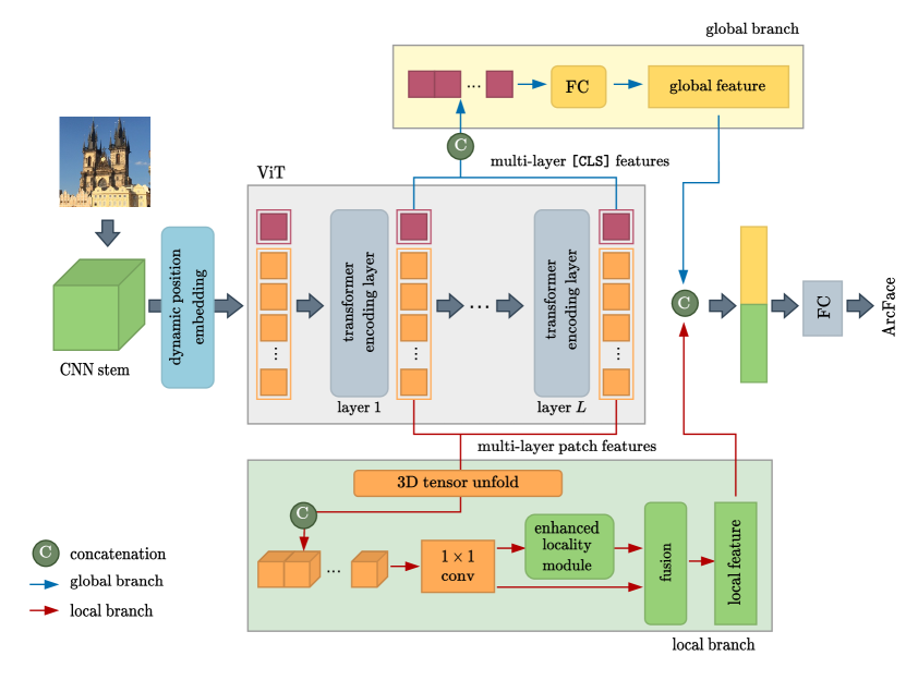
Figure 1: The high-level design of our deep token pooling (DToP). Using a transformer encoder (center), we build a global image representation for image retrieval by means of a global branch (blue arrows, top) and a local branch (red arrows, bottom), collecting [CLS] and patch token embeddings, respectively, from multiple layers. There are two mechanisms to improve locality of interactions (green): a CNN stem for the first layers (left), which amounts to a hybrid architecture, and our enhanced locality module (ELM) (Figure 2(b)) in the local branch. Our dynamic position embedding (DPE) (Figure 2(a)) allows for dynamic image size at training.

2.1 Preliminaries: vision transformer

A transformer encoder, shown in the center of Figure 1, processes a sequence of token embeddings by allowing pairwise interactions in each layer. While we investigate a number of vision transformers, we follow ViT [29] here, which is our default choice. The input sequence can be written as

$$X=[\mathbf{x}_{\texttt{[CLS]}};\mathbf{x}_{1};\dots;\mathbf{x}_{M}]\in{}^{(M+1)\times D},$$ (1)

where patch token embeddings $\mathbf{x}_{1},\dots,\mathbf{x}_{M}\in{}^{D}$ are obtained from the input image, the learnable [CLS] token embedding $\mathbf{x}_{\texttt{[CLS]}}$ serves as global image representation at the output layer, $M$ is the sequence length and $D$ is the token embedding dimension.

There are two ways to form patch token embeddings. The most common is to decompose the input image into $M=wh$ raw, fixed-size, square non-overlapping patches and project them to $D$ dimensions via a learnable linear layer. Alternatively, one may use a convolutional network stem to map the raw input image to a $w\times h\times D$ feature tensor, then fold this tensor into a sequence of $M=wh$ vectors of dimension $D$. This is called a hybrid architecture. Here, $w\times h$ is input resolution, i.e., the image resolution divided by the patch size in the first case or the downsampling ratio of the stem in the second.

The input sequence is added to a sequence of learnable position embeddings, meant to preserve positional information, and given to the transformer encoder, which has $L$ layers preserving the sequence length and dimension. Each layer consists of a multi-head self attention (MSA) and an MLP block. The output is the embedding of the [CLS] token at the last layer, $\mathbf{c}^{L}$.

2.2 Motivation and design principles

We are investigating a number of ideas, discussing related work in other tasks and laying out design principles accordingly. The overall goal is to use the features obtained by a vision transformer, without designing an entirely new architecture or extending an existing one too much.

Hybrid architecture

As shown in the original ViT study [29], hybrid models slightly outperform ViT at small computational budgets, but the difference vanishes for larger models. Of course, this finding refers to image classification tasks only. Although hybrid models are still studied [17], they are not mainstream: It is more common to introduce structure and inductive bias to transformer models themselves, where the input is still raw patches [37, 23, 62, 67, 19].

We are the first to conduct a large-scale investigation of different transformer architectures including hybrid models for image retrieval. Interestingly, we find that, in terms of global representation like the [CLS] token embeddings, the hybrid model originally introduced by [29] and consisting of a CNN stem and a ViT encoder performs best on image retrieval benchmarks by a large margin. As shown on the left in Figure 1, we use a CNN stem and a ViT encoder by default: The intermediate feature maps of the CNN stem are fed into ViT as token embeddings with patch size $1\times 1$ rather than raw image patches.

Handling different image resolutions

Image resolutions is an important factor in training image retrieval models. It is known that preserving original image resolution is effective [20, 16]. However, this leads to increased computational cost and longer training time. Focusing on image classification, MobileViT [38] proposes a multi-scale sampler that randomly samples a spatial resolution from a fixed set and computes the batch size for this resolution at every training iteration. On image retrieval, group-size sampling [65] has been shown very effective. Here, one constructs a mini batch with images of similar aspect ratios, resizing them to a prefixed size according to aspect ratio.

We follow this latter approach. However, because of different aspect ratio, the image size is still different per mini-batch, which presents a new challenge: Position embeddings are of fixed length, corresponding to fixed spatial resolution when unfolded. For this reason, as shown on the left in Figure 1, we propose dynamic position embedding (DPE), whereby the fixed-size learned embeddings are dynamically resampled to the size of each mini-batch.

Global and local branches

It is well known [42, 48, 39] that an image retrieval model should focus on the target object, not the background. It is then no surprise that recent methods, focusing either on global or local representations, have a global and a local branch in their architecture after the backbone [3, 56, 61, 64, 53]. The objective of the local branch is to improve the localization properties of the model, even if the representation is eventually pooled into a single vector. Even though transformers have shown better localization properties than convolutional networks, especially in the self-supervised setting [4, 22, 33], the few studies so far on vision transformers for image retrieval are limited to using the [CLS] token from the last layer of ViT as a global representation [12, 4, 14].

In this context, our goal is to investigate the role of a local branch on top of a vision transformer encoder for image retrieval. This study is unique in that the local branch has access to patch token embeddings of different layers, re-introduces inductive bias by means of convolution at different scales and ends in global spatial pooling, thereby being complementary to the [CLS] token. As shown on the top/bottom in Figure 1, the global/local branch is based on the [CLS]/patch tokens, respectively. The final image representation is based on the concatenation of the features generated by the two branches.

Multi-layer features

It is common in object detection, semantic segmentation and other dense prediction tasks to use features of different scales from different network layers, giving rise to feature pyramids [50, 36, 35, 34, 55]. It is also common to introduce skip connections within the architecture, sparsely or densely across layers, including architecture learning [24, 71, 13]. Apart from standard residual connections, connections across distant layers are not commonly studied in either image retrieval or vision transformers.

As shown on the top/bottom in Figure 1, without changing the encoder architecture itself, we investigate direct connections from several of its last layers to both the global and local branches, in the form of concatenation followed by a number of layers. This is similar to hypercolumns [21], but we are focusing on the last layers and building a global representation. The spatial resolution remains fixed in ViT, but we do take scale into account by means of dilated convolution. Interestingly, skip connections and especially direct connections to the output are known to improve the loss landscape of the network [31, 40].

Enhancing locality

The transformers mainly rely on global self-attention, which makes them good at modeling long-range dependencies. However, contrary to convolutional networks with fixed kernel size, they lack a mechanism to localize interactions. As a consequence, many studies [70, 66, 19, 32, 7, 43, 5] are proposed to improve ViT by bringing in locality.

In this direction, apart from using a CNN stem in the first layers, we introduce an enhanced locality module (ELM) in the local branch, as shown in Figure 1. Our goal is to investigate inductive bias in the deeper layers of the encoder, without overly extending the architecture itself. For this reason, the design of ELM is extremely lightweight, inspired by mobile networks [51].

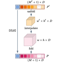
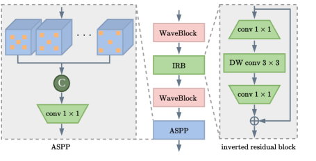
(a) dynamic position	(b) enhanced locality module
embedding

Figure 2: (a) Our dynamic position embedding (DPE) adapts learnable position embeddings of fixed size $(M^{\prime}+1)\times D$ to dynamic size $(M+1)\times D$, when using images of different size per mini-batch. (b) Our enhanced locality module (ELM) in the local branch enhances locality of interactions and consists of an inverted residual block (IRB), an à trous spatial pyramid pooling (ASPP) and two WaveBlock layers.

2.3 Detailed model

According to the design principles discussed above, we provide a detailed account of our full model. In our ablation study (subsection 3.4), ideas and components are assessed individually.

Dynamic position embedding (DPE)

The position embeddings of the transformer encoder (subsection 2.1) are represented by a learnable matrix $P$ that is assumed to be of the same size as the input sequence $X$, that is, $(M+1)\times D$. When image size is different in each mini-batch, the input resolution $w\times h$ and $M=wh$ are also different. But how can $P$ change size while being learnable, that is, maintained across mini-batches?

We address this inconsistency by actually representing the position embeddings by a learnable matrix $P^{\prime}=[\mathbf{p}_{\texttt{[CLS]}};\mathbf{p}^{\prime}_{1};\dots;\mathbf{p}^{\prime}_{M^{\prime}}]$ of fixed size $(M^{\prime}+1)\times D$, where $M^{\prime}=w^{\prime}h^{\prime}$ and $w^{\prime}\times h^{\prime}$ is some fixed spatial resolution. As shown in Figure 2(a), at each mini-batch, the sequence $\mathbf{p}^{\prime}_{1},\dots,\mathbf{p}^{\prime}_{M^{\prime}}$ corresponding to the patch tokens is unfolded to a $w^{\prime}\times h^{\prime}\times D$ tensor, then interpolated and resampled as $w\times h\times D$, and finally folded back to a new sequence $\mathbf{p}_{1},\dots,\mathbf{p}_{M}$. Pre-pending $\mathbf{p}_{\texttt{[CLS]}}$ again, which remains unaffected, yields the position embedding

$$P=[\mathbf{p}_{\texttt{[CLS]}};\mathbf{p}_{1};\dots;\mathbf{p}_{M}]$$ (2)

of dynamic size $(M+1)\times D$ per mini-batch. We call this method dynamic position embedding (DPE).

Multi-layer [CLS]/patch features

The input sequence $X$ and the position embedding sequence $P$ are first added

$$Z^{0}=X+P=[\mathbf{z}_{\texttt{[CLS]}}^{0};\mathbf{z}_{1}^{0};\dots;\mathbf{z}_{M}^{0}]\in{}^{(M+1)\times D}.$$ (3)

This new sequence is the input to the transformer encoder. Let $f^{\ell}:{}^{(M+1)\times D}\to{}^{(M+1)\times D}$ be the mapping of layer $\ell$ of the encoder and

$$Z^{\ell}=f^{\ell}(Z^{\ell-1})=[\mathbf{z}_{\texttt{[CLS]}}^{\ell};\mathbf{z}_{1}^{\ell};\dots;\mathbf{z}_{M}^{\ell}]\in{}^{(M+1)\times D}$$ (4)

be its output sequence, for $\ell=1,\dots,L$, where $L$ is the number of layers.

Given a hyper-parameter $k\in\{1,\dots,L\}$, multi-layer [CLS] and patch features are collected from the sequences $Z^{L-k+1},\dots,Z^{L}$ of the last $k$ layers:

$$F_{c} =[\mathbf{z}_{\texttt{[CLS]}}^{L-k+1};\dots;\mathbf{z}_{\texttt{[CLS]}}^{L}]\in{}^{k\times D}$$ (5)

$$F_{p} =[A^{L-k+1};\dots;A^{L}]\in{}^{k\times w\times h\times D},$$ (6)

where $A^{\ell}\in{}^{w\times h\times D}$ is the sequence $\mathbf{z}_{1}^{\ell},\dots,\mathbf{z}_{M}^{\ell}$ of patch token embeddings of layer $\ell$, unfolded into a $w\times h\times D$ tensor, recalling that $M=wh$.

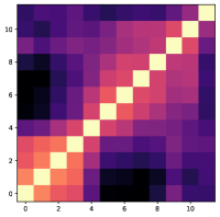
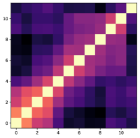
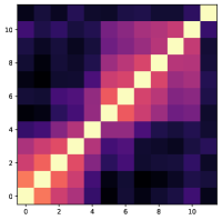
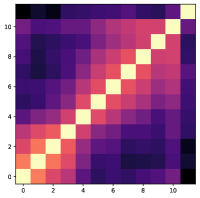
(a) NC-clean	(b) SfM-120k	(c) GLDv1-noisy	(d) GLDv2-clean

Figure 3: Centered kernel alignment (CKA) [41, 49] heatmap between all pairs of transformer encoding layers of our models trained on different datasets (subsection 3.1). For a given pair of layers, CKA is the correlation coefficient of the Gram matrices of the feature tensors of the two layers, averaged over the training set.

Apart from the ablation on $k$ in subsection 3.4, can we already get an idea whether $k>1$ is meaningful? From Figure 3, the answer is yes. Layers 1-4 and 6-11 tend to group by correlation, while layer 5 is correlated with both groups. It is thus not clear which of the layers 1-11 stand out as more distinctive. What is crystal clear is that the last layer 12 is totally uncorrelated with all others.

Global and local branches

The global branch, shown above the encoder in Figure 1, takes as input the multi-layer [CLS] features $F_{c}$ (5) and embeds them in a $N$-dimensional space

$$\mathbf{u}_{c}=\textsc{fc}(F_{c})\in{}^{N}.$$ (7)

using a fully connected layer (FC). The local branch, shown below the encoder in Figure 1, takes as input the multi-layer patch features $F_{p}$ (6), containing rich spatial information. We apply $1\times 1$ convolution to reduce the number of channels effectively from $kD$ to $D$:

$$Y=\operatorname{conv}_{1\times 1}(F_{p})\in{}^{w\times h\times D}$$ (8)

Then, we apply our enhanced locality module (ELM), described below, and we fuse with $Y$, choosing from a number of alternative functions studied in the supplementary:

$$Y^{\prime}=\textsc{fuse}(Y,\textsc{elm}(Y))\in{}^{w\times h\times D},$$ (9)

We obtain an $N$-dimensional embedding from the local branch by global average pooling (GAP) over the spatial dimensions ($w\times h$), followed by an FC layer:

$$\mathbf{u}_{p}=\textsc{fc}(\textsc{gap}(Y^{\prime}))\in{}^{N}.$$ (10)

Enhanced locality module (ELM)

As shown in Figure 2, our enhanced locality module (ELM) consists of an inverted residual block (IRB) [51] followed by à trous spatial pyramid pooling (ASPP) [6]. IRB is wrapped by two WaveBlock (WB) [58] layers, serving as feature-level augmentation:

$$\textsc{elm}(Y)=\textsc{aspp}(\textsc{wb}(\textsc{irb}(\textsc{wb}(Y))))\in{}^{w\times h\times D}.$$ (11)

IRB is a lightweight convolutional layer, where convolution is separable over the spatial and channel dimensions. In particular, it consists of a $1\times 1$ convolution (expansion from $D$ to $D^{\prime}>D$), a $3\times 3$ depthwise convolution and another $1\times 1$ convolution (squeeze from $D^{\prime}$ to $D$) layer. ASPP acquires multi-scale spatial context information: Feature maps obtained by à trous (dilated) convolution at multiple dilation rates $r_{1},\dots,r_{n}$ are concatenated and reduced back from $nD$ to $D$ dimensions by a $1\times 1$ convolution.

Image representation

Finally, as shown on the right of Figure 1, we obtain a global $N$-dimensional image representation by concatenating $\mathbf{u}_{c}$ (7) with $\mathbf{u}_{p}$ (10) and applying dropout, a fully connected layer and batchnorm (BN):

$$\mathbf{u}=\textsc{bn}(\textsc{fc}(\textsc{dropout}([\mathbf{u}_{c};\mathbf{u}_{p}])))\in{}^{N},$$ (12)

reducing the dimensions from $2N$ to $N$.

3 Experiments

3.1 Setup

Training sets

There are a number of open landmark datasets commonly used for training in image retrieval studies, including neural code (NC) [2], structure-from-motion 120k (SfM-120k) [48], Google landmarks v1 (GLDv1) [42] and v2 (GLDv2) [60]. Most of these datasets are noisy because they were obtained by text search. For example, many images contain no landmarks. Clean sets are also available where noise has has been removed in different ways [16, 48, 60]. Overall, we use NC-clean, SfM-120k, GLDv1-noisy and GLDv2-clean as training sets in our experiments. More details are in the supplementary.

Evaluation sets/metrics

We use Oxford5 (Ox5k) [44], Paris6k (Par6k) [45], Revised Oxford ($\mathcal{R}$Oxford or $\mathcal{R}$Oxf), and Paris ($\mathcal{R}$Paris or $\mathcal{R}$Par) [46] as evaluation sets in our experiments. We also use one million distractors ($\mathcal{R}$1M) [46] in some experiments. We use the Medium and Hard protocols of [46]. Performance is measured by mean Average Precision (mAP) and mean precision at 10 (mP@10).

Architecture

The architecture is chosen as R50+ViT-B/16 [29] with 98M parameters, pre-trained on ImageNet-21k [10]. That is, we use Resnet50 as CNN stem and ViT-B/16 as transformer encoder. Factor 16 is the downsampling ratio of the stem. Through all encoder layers, the embedding dimension is $D=768$, the default of ViT-B. The additional components of DToP have only 0.3M parameters. The choice of architecture is among 15 candidates (14 vision transformers and the selected hybrid model), of which we benchmarked 12 by training on SfM-120k and measuring retrieval performance using global features, as detailed in the supplementary.

Implementation details

We conduct a detailed ablation study in subsection 3.4 and in the supplementary. Default settings are as follows. The number of multi-layer features (5),(6) is $k=6$. The set of dilation rates $\{r_{1},\dots,r_{n}\}$ of ASPP (11) is $\{6,12,18\}$. The dimension of the output feature vector $\mathbf{u}$ is $N=1,536$. Training settings are detailed in the supplementary. Supervised whitening [48] is applied except for GLDv2-clean, where the performance drops. At inference, the batch normalization of (12) is removed and we adopt a multi-scale representation using 3 scales [16, 48]. We do not consider local descriptor matching [42, 52, 3, 56, 46] or re-ranking [26, 63].

3.2 Main results

Table 1 compares our deep token pooling (DToP) models against the state of the art (SOTA), grouped by representation type (global or local descriptors) and by training set. We use a global descriptor, so local descriptors should be for reference only, but we do make some comparisons to show that a better training set or model can compensate for a larger representation. To the best of our knowledge, we are the first to organize results by training set and train a model on all commonly used training sets in the literature for fair comparison. More results are in the supplementary, including re-ranking with diffusion [26].

Method					Base		Medium								Hard
					Ox5k	Par6k	$\mathcal{R}$Oxf		$\mathcal{R}$Oxf +$\mathcal{R}$1M		$\mathcal{R}$Par		$\mathcal{R}$Par +$\mathcal{R}$1M		$\mathcal{R}$Oxf		$\mathcal{R}$Oxf +$\mathcal{R}$1M		$\mathcal{R}$Par		$\mathcal{R}$Par +$\mathcal{R}$1M
					mAP	mAP	mAP	mP@10	mAP	mP@10	mAP	mP@10	mAP	mP@10	mAP	mP@10	mAP	mP@10	mAP	mP@10	mAP	mP@10
Local Descriptors (NC-clean)
DELF-DIR-R101 [42]					90.0	95.7	–	–	–	–	–	–	–	–	–	–	–	–	–	–	–	–
Local Descriptors (SfM-120k)
DELF-ASMK-SP [46]					–	–	67.8	87.9	–	–	76.9	99.3	–	–	43.1	62.4	–	–	55.4	93.4	–	–
DSM-MAC-R101 [52]					–	–	62.7	83.7	44.4	72.3	75.7	98.7	50.4	96.4	35.4	51.6	20.6	32.3	53.1	88.6	22.7	72.1
DSM-GeM-R101 [52]					–	–	65.3	87.1	47.6	76.4	77.4	99.1	52.8	96.7	39.2	55.3	23.2	37.9	56.2	89.9	25.0	74.6
HOW-ASMK-R50 [56]					–	–	79.4	–	–	–	81.6	–	–	–	56.9	–	–	–	62.4	–	–	–
FIRe-R50 [59]					–	–	81.8	–	66.5	–	85.3	–	67.6	–	61.2	–	40.1	–	70.0	–	42.9	–
MDA-R50 [61]					–	–	81.8	–	68.7	–	83.3	–	64.7	–	62.2	–	45.3	–	66.2	–	38.9	–
Local Descriptors (GLDv2-clean)
DELG-GeM-R50 [3]					–	–	78.3	–	67.2	–	85.7	–	69.6	–	57.9	–	43.6	–	71.0	–	45.7	–
DELG-GeM-R101 [3]					–	–	81.2	–	69.1	–	87.2	–	71.5	–	64.0	–	47.5	–	72.8	–	48.7	–
RRT-R50 [54]					–	–	78.1	–	67.0	–	86.7	–	69.8	–	60.2	–	44.1	–	75.1	–	49.4	–
Global Descriptors (Off-the-shelf, pre-trained on ImageNet)
SPoC-V16 [1, 46]					53.1	–	38.0	54.6	17.1	33.3	59.8	93.0	30.3	83.0	11.4	20.9	0.9	2.9	32.4	69.7	7.6	30.6
SPoC-R101 [46]					–	–	39.8	61.0	21.5	40.4	69.2	96.7	41.6	92.0	12.4	23.8	2.8	5.6	44.7	78.0	15.3	54.4
MAC-V16 [47, 46]					80.0	82.9	37.8	57.8	21.8	39.7	59.2	93.3	33.6	87.1	14.6	27.0	7.4	11.9	35.9	78.4	13.2	54.7
MAC-R101 [46]					–	–	41.7	65.0	24.2	43.7	66.2	96.4	40.8	93.0	18.0	32.9	5.7	14.4	44.1	86.3	18.2	67.7
RMAC-V16 [47, 46]					80.1	85.0	42.5	62.8	21.7	40.3	66.2	95.4	39.9	88.9	12.0	26.1	1.7	5.8	40.9	77.1	14.8	54.0
RMAC-R101 [46]					–	–	49.8	68.9	29.2	48.9	74.0	97.7	49.3	93.7	18.5	32.2	4.5	13.0	52.1	87.1	21.3	67.4
DINO-R50 [4]					–	–	35.4	–	–	–	55.9	–	–	–	11.1	–	–	–	27.5	–	–	–
DINO-ViT-S [4]					–	–	41.8	–	–	–	63.1	–	–	–	13.7	–	–	–	34.4	–	–	–
ViT-B [14]					64.7	87.8	–	–	–	–	–	–	–	–	–	–	–	–	–	–	–	–
Global Descriptors (NC-clean)
RMAC-R101 [16, 46]					86.1	94.5	60.9	78.1	39.3	62.1	78.9	96.9	54.8	93.9	32.4	50.0	12.5	24.9	59.4	86.1	28.0	70.0
GLAM-R101 [53]					77.8	85.8	51.6	–	–	–	68.1	–	–	–	20.9	–	–	–	44.7	–	–	–
DOLG-R101 [64]†					73.1	79.5	47.0	67.1	–	–	61.5	92.1	–	–	20.0	33.7	–	–	33.1	68.3	–	–
DToP-R50+ViT-B (ours)					86.2	92.9	64.8	81.3	46.5	64.3	82.0	96.4	54.6	92.9	41.3	56.9	21.5	36.6	63.2	87.4	28.9	66.9
Global Descriptors (GLDv1-noisy)
SOLAR-R101 [39]					–	–	69.9	86.7	53.5	76.7	81.6	97.1	59.2	94.9	47.9	63.0	29.9	48.9	64.5	93.0	33.4	81.6
GeM-R101 [60]					–	–	68.9	–	–	–	83.4	–	–	–	45.3	–	–	–	67.2	–	–	–
GLAM-R101 [53]					92.8	95.0	73.7	–	–	–	83.5	–	–	–	49.8	–	–	–	69.4	–	–	–
DINO-DeiT-S [4]					–	–	51.5	–	–	–	75.3	–	–	–	24.3	–	–	–	51.6	–	–	–
DToP-R50+ViT-B (ours)					88.8	95.7	71.6	85.1	55.8	75.9	88.7	96.6	67.8	95.6	51.7	65.1	30.9	49.3	75.9	90.4	44.1	82.0
Global Descriptors (SfM-120k)
RMAC-R101 [16]‡					79.0	86.3	53.5	76.9	–	–	68.3	97.7	–	–	25.5	42.0	–	–	42.4	83.6	–	–
GeM-A [48, 46]					67.7	75.5	43.3	62.1	24.2	42.8	58.0	91.6	29.9	84.6	17.1	26.2	9.4	11.9	29.7	67.6	8.4	39.6
GeM-V16 [48, 46]					87.9	87.7	61.9	82.7	42.6	68.1	69.3	97.9	45.4	94.1	33.7	51.0	19.0	29.4	44.3	83.7	19.1	64.9
GeM-R101 [48, 46]					87.8	92.7	64.7	84.7	45.2	71.7	77.2	98.1	52.3	95.3	38.5	53.0	19.9	34.9	56.3	89.1	24.7	73.3
AGeM-R101 [18]					–	–	67.0	–	–	–	78.1	–	–	–	40.7	–	–	–	57.3	–	–	–
SOLAR-R101 [39]†					78.5	86.3	52.5	73.6	–	–	70.9	98.1	–	–	27.1	41.4	–	–	46.7	83.6	–	–
GeM-R101 [60]†					79.0	82.6	54.0	72.5	–	–	64.3	92.6	–	–	25.8	42.2	–	–	36.6	67.6	–	–
GLAM-R101 [53]‡					89.7	91.1	66.2	–	–	–	77.5	–	–	–	39.5	–	–	–	54.3	–	–	–
DOLG-R101 [64]†					72.8	74.5	46.4	66.8	–	–	56.6	91.1	–	–	18.1	27.9	–	–	26.6	62.6	–	–
IRT-DeiT-B [12]					–	–	55.1	–	–	–	72.7	–	–	–	28.3	–	–	–	49.6	–	–	–
DToP-R50+ViT-B (ours)					89.7	92.7	68.5	85.4	48.9	71.7	83.1	96.4	56.5	94.0	43.0	56.9	24.7	38.9	65.8	89.1	30.3	69.6
Global Descriptors (GLDv2-clean)
GeM-R101 [60]					–	–	76.2	–	–	–	87.3	–	–	–	55.6	–	–	–	74.2	–	–	–
GLAM-R101 [53]					94.2	95.6	78.6	88.2	68.0	82.4	88.5	97.0	73.5	94.9	60.2	72.9	43.5	62.1	76.8	93.4	53.1	84.0
DELG-GeM-R50 [3]					–	–	73.6	–	60.6	–	85.7	–	68.6		51.0	–	32.7	–	71.5	–	44.4	–
DELG-GeM-R101 [3]					–	–	76.3	–	63.7	–	86.6	–	70.6		55.6	–	37.5	–	72.4	–	46.9	–
DOLG-R50 [64]					–	–	80.5	–	76.6	–	89.8	–	80.8	–	58.8	–	52.2	–	77.7	–	62.8	–
DOLG-R101 [64]					–	–	81.5	–	77.4	–	91.0	–	83.3	–	61.1	–	54.8	–	80.3	–	66.7	–
DOLG-R101 [64]∃					95.5	95.9	78.8	91.6	64.2	82.1	87.8	96.6	68.7	94.1	58.0	74.8	37.3	57.7	74.1	91.1	45.1	80.0
DToP-R50+ViT-B (ours)					95.0	97.0	82.1	91.7	70.9	83.9	92.0	96.6	81.9	96.4	64.5	77.4	49.0	66.6	82.9	94.3	64.0	90.6
DOLG-R101 [64]∃□					91.7	96.2	79.3	93.2	71.3	89.1	89.2	98.9	74.7	97.7	57.2	73.0	43.4	62.6	76.6	94.1	53.6	89.7
DToP-R50+ViT-B (ours)□					94.2	97.6	84.4	94.1	78.9	91.3	92.3	97.1	85.4	96.9	64.8	76.7	57.1	72.1	84.6	95.4	71.2	94.6

Table 1: mAP comparison by local/global descriptors and by training set; comparison of our DToP vs. global descriptor SOTA per training set. Bold: best results per training set. A: AlexNet; V16: VGG16; R50/101:Resnet50/101. By default, all competitor results are as reported by authors. $\dagger/\ddagger$: training using official/our code; $\exists$: evaluation using official pre-trained model; $\square$: non-cropped queries.

Comparisons with global descriptors

Under global descriptors and all training sets, we achieve SOTA performance in almost all evaluation cases. We do not use local descriptor based re-ranking [42, 3, 52, 54] or aggregation [56, 46], or any other re-ranking such as diffusion [26, 63]. Of course, as detailed in the supplementary, our model is not comparable to others in terms of backbone or pre-training, but it is our objective to advance vision transformers on image retrieval without introducing a new architecture.

On GLDv2-clean, comparing with published results of DOLG [64], we improve by 0.7%, 1.0% on $\mathcal{R}$Oxf, $\mathcal{R}$Par Medium and by 7.6%, 7.8% on $\mathcal{R}$Oxf, $\mathcal{R}$Par Hard. DOLG is still better on $+$$\mathcal{R}$1M, but we have not been able to reproduce the published results using the official pre-trained model and the same problem has been encountered by the community. This may be due to having used non-cropped queries or not; the official code uses non-cropped queries by default, which is against the protocol [46]. By evaluating the DOLG official pre-trained model, we outperform it on all datasets except Ox5k. For completeness, we also report non-cropped queries for both DOLG and our DToP separately, where again we outperform DOLG on all datasets.

Comparisons with vision transformer studies

Such studies are only few [14, 12, 4, 54]. They all use global descriptors, except [54], which uses a transformer to re-rank features obtained by CNN rather than to encode images. On global descriptors/SfM-120k, comparing with IRT [12], we improve by 13.4%, 10.4% on $\mathcal{R}$Oxf, $\mathcal{R}$Par Medium and by 14.7%, 16.2% on $\mathcal{R}$Oxf, $\mathcal{R}$Par Hard. On local descriptors/GLDv2-clean, comparing with RRT [54], we improve by 6.3%, 5.3% on $\mathcal{R}$Oxf, $\mathcal{R}$Par Medium and by 4.3%, 7.8% on $\mathcal{R}$Oxf, $\mathcal{R}$Par Hard. This shows the advantage of our model over the local descriptors of RRT.

Comparisons with local descriptor aggregation

Studies using local descriptors generally work better at the cost of more memory and more complex search process. Our study is not of this type, but we do show better performance results if we allow different training sets—which has been the norm before our work. Comparing our DToP on GLDv2 with HOW [56] on SfM-120k, we improve by 2.7%, 10.4% on $\mathcal{R}$Oxf, $\mathcal{R}$Par Medium and by 3.4%, 20.5% on $\mathcal{R}$Oxf, $\mathcal{R}$Par Hard. On the same training set (SfM-120k), we improve on $\mathcal{R}$Par but lose on $\mathcal{R}$Oxf. We also lose from very recent improvements [61, 59].

Comparisons with local descriptor-based re-ranking

Such methods first filter by global descriptors, then re-rank candidates by local descriptors, which is even more complex than local descriptor aggregation. On GLDv2-clean, comparing with DELG [3], we improve by 0.9%, 4.8% on $\mathcal{R}$Oxf, $\mathcal{R}$Par Medium and by 0.5%, 10.1% on $\mathcal{R}$Oxf, $\mathcal{R}$Par Hard.

Dim	Oxf5k	Par6k	Medium		Hard
			$\mathcal{R}$Oxf	$\mathcal{R}$Par	$\mathcal{R}$Oxf	$\mathcal{R}$Par
DINO (ViT-S) [4]	–	–	51.5	75.3	24.3	51.6
IRT (DeiT-B) [12]	–	–	55.1	72.7	28.3	49.6
Ours (DeiT-B)	85.9	90.1	62.3	78.1	33.6	54.5
Ours (ViT-B)	89.7	92.7	68.5	83.1	43.0	65.8

Table 2: mAP comparison of our model with previous approaches using vision transformers as backbones for retrieval. Training on SfM-120k.

Image retrieval using vision transformers

In Table 2, we compare with the few previous approaches using vision transformers as backbones for image retrieval, to highlight our progress. Both [12, 4] use global descriptors from the same transformer encoder like we do, although they use different pre-training settings. Our improvement by 10-20% mAP is significant progress.

3.3 Visualization

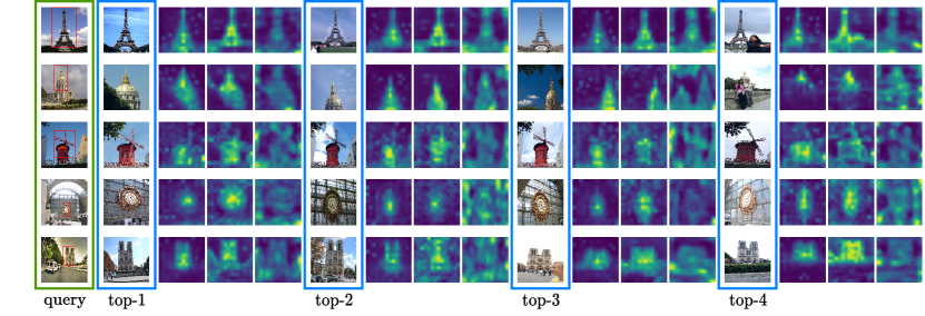
Figure 4: Examples of ranking by our model and spatial attention. On the left (green box) is the query, followed by 4 top-ranking results, including images (blue box) attention maps by our DToP (full model), our baseline model (Table 3) and Resnet101. For our transformer model (full and baseline), we show the attention map between the [CLS] and all the other tokens. For Resnet we do the same, using GAP to obtain a vector that plays the role of the [CLS] token embedding.

Ranking and spatial attention

Figure 4 shows examples, for a number of queries, of the top-ranking images by our DToP, along with attention maps. Our model is attending only the object of interest, not the background. Whereas, Resnet101 is also attending the background to a great extent. Our full model also attends more clearly the foreground than the baseline. More visualizations are given in the supplementary, including t-SNE embeddings.

3.4 Ablation study

Unless otherwise stated, all ablation experiments are conducted on SfM-120k. Additional experiments are in the supplementary, including experiments on 13 different transformer backbones, the number of layers $k$, DPE against baselines, ELM components, the feature dimension $N$, mini-batch sampling, multi-scale features at inference as well as fusion alternatives for (9).

Design/algorithmic ablation

We assess the effect of different choices and components to the performance of our model. Our baseline is the plain ViT-B/16 transformer using raw patch tokens, with a plain [CLS] token representation from the last layer ($F_{c}=\mathbf{z}_{\texttt{[CLS]}}^{L}$), mapped to $N$ dimensions by an FC layer (7). The baseline is trained with group-size sampling [65] and our DPE (2); this setting is ablated separately. Adding the CNN stem amounts to switching to R50+ViT-B/16 hybrid model. Adding the local and global branches includes multi-layer [CLS] (5) and patch (6) features respectively, where the local branch replaces the plain [CLS] token representation ($F_{c}=\mathbf{z}_{\texttt{[CLS]}}^{L}$) by (5) when present. In (12), only $\mathbf{u}_{c}$ (7), $\mathbf{u}_{p}$ (10) is present when only the global, local branch is present respectively. Removing ELM amounts to setting $Y^{\prime}=Y$ in (9).

CNN	global	local		ELM	Oxf5k	Par6k	Medium		Hard
Stem	branch	branch					$\mathcal{R}$Oxf	$\mathcal{R}$Par	$\mathcal{R}$Oxf	$\mathcal{R}$Par
					77.7	85.9	52.6	76.0	26.6	52.0
	✓				76.6	87.3	54.7	77.0	27.7	54.8
	✓	✓			78.3	89.7	57.9	78.2	24.2	54.4
	✓	✓		✓	81.5	89.8	61.4	79.7	32.5	57.4
✓					81.2	86.4	55.5	76.2	31.4	52.1
✓	✓				88.3	91.9	66.6	83.6	41.9	67.8
✓	✓	✓			89.8	91.2	67.6	81.1	40.7	62.5
✓	✓	✓		✓	89.7	92.7	68.5	83.1	43.0	65.8

Table 3: mAP comparison of variants of our model with/without different components. Training on SfM-120k. ELM: enhanced locality module (11).

As shown in Table 3, the greatest improvement comes from the CNN stem when combined with the global branch, confirming the importance of the inductive bias of convolution in the early layers and the complementarity of the [CLS] features of the last layers. In the absence of the CNN stem, each component (global/local branch, ELM) is improving the performance. By contrast, when the CNN stem is present, the contribution of the local branch and ELM is inconsistent across $\mathcal{R}$Oxf and $\mathcal{R}$Par. These two components can thus be thought as lightweight alternatives to the CNN stem, improving locality in the last layers.

4 Conclusion

We have introduced a new approach to leverage the power of vision transformers for image retrieval, reaching or setting new state of the art with global representations for the first time. By collecting both global and local features from multiple layers and enhancing locality in the last layers, we learn powerful representations that have improved localization properties, in the sense of attending the object of interest. Some of our ideas may be applicable beyond transformers and beyond retrieval. Our unexpected finding that a hybrid architecture outperforms most transformers by a large margin may open new directions in architecture design. A very interesting future direction is self-supervised learning of transformers for retrieval.

Appendix A More experiments

A.1 Setup

Network size and pretraining

The ViT-B transformer encoder and the R50+ViT-B hybrid have 86M and 98M parameters respectively and are pretrained on ImageNet-21k. The additional components of DToP have only 0.3M parameters. The common competitors Resnet50/101 have 25M and 44M parameters respectively and are pretrained on ImageNet-1k. Despite its lower dimensionality (1,536 vs. 2,048 dimensions for Resnet101), our DToP-R50+ViT-B is of course in a priviledged position over Resnet101 in terms of both network size and pretraining data. Still, it is important that a transformer reaches SOTA on image retrieval for the first time. Our objective is not to introduce a new architecture.

Training settings

We apply random cropping, illumination and scaling augmentation. We use a batch size of 64 and the ArcFace loss with margin 0.15. We optimize by stochastic gradient descent with momentum 0.9, initial learning rate $10^{-3}$ and cosine learning rate decay with the decay factor $10^{-4}$. We apply warm-up of 0, 3, 5 and 5 epochs on NC-clean, SfM-120k, GLDv1-noisy and GLDv2-clean, respectively. We implement our method on PyTorch and we train our models on 8 TITAN RTX 3090Ti GPUs.

A.2 Benchmarking of vision transformer models

Vision transformer studies have exploded in a short period of time, but very few concern image retrieval. We perform for the first time an extensive empirical study to benchmark a large number of vision transformer models on image retrieval and choose the best performing one as our default backbone.

Candidate models

We fine-tune on image retrieval training sets, so we only consider models that are pre-trained on ImageNet-1k or ImageNet-21k [10]. In particular, we consider the models shown in Table 4.

As global image representation, all models use a [CLS] (classification) token embedding, while PiT [23] and DeiT [25] also provide a distillation token embedding. As a local image representation, patch token embeddings can be used for all models, while for the hybrid R50+ViT-B, features of the CNN stem can also be used. Certain pre-trained models, in particular Swin [37], ConViT [9] and TNT [19], cannot handle multi-scale input. These models are not compatible with the group-size sampling approach that we adopt for training [65]. This constraint is not due to the architecture itself but to the way the code is written, and although it would be certainly possible to fix, this would require some effort. We therefore exclude them from our benchmark.

Model	CLS	Dist	Patch	CNN	MS
Swin [37]	✓		✓
ConViT [9]	✓		✓
TNT [19]	✓		✓
ViL [68]	✓		✓		✓
CvT [62]	✓		✓		✓
LocalViT [32]	✓		✓		✓
Patch [15]	✓		✓		✓
T2T [67]	✓		✓		✓
DeepViT [69]	✓		✓		✓
LV-ViT [27]	✓		✓		✓
PiT [23]	✓	✓	✓		✓
DeiT (DeiT-B) [25]	✓	✓	✓		✓
ViT (ViT-B) [29]	✓		✓		✓
ViT (R50+ViT-B)	✓		✓	✓	✓

Table 4: Feature types that can be extracted from different pre-trained vision transformer models considered in our study. CLS: classification token; Dist: distillation token; Patch: patch tokens. CNN: convolutional stem (hybrid model). MS: can handle multi-scale input at training (required in our experiments).

Setup

We take all models as pre-trained on either ImageNet-1k or ImageNet-21k and fine-tune them on SfM-120k [48]. We use only the global branch (7) on multi-layer [CLS] features (5) or the local branch (10) on multi-layer patch features (6). In the former case, we also evaluate multi-layer distillation features, replacing [CLS] by the distillation token where it exists, i.e., PiT [23] and DeiT [25]. In the latter case, we do not use the enhanced locality module (ELM), that is, we set $Y^{\prime}=Y$ in (9). At the output, instead of (12), we only use an FC layer with output feature dimension $N=768$. We use group-size sampling [65] with our dynamic position embedding (DPE) (2). We use default training settings, except without warm-up.

At inference, we evaluate each model with exactly the same type of features as at training ([CLS], distillation or patch), applying supervised whitening [48] on multi-scale features [48] and measuring mAP on the evaluation sets.

Model	Pre-Train	Params (M)	Global (CLS/Dist)							Local (Patch)
			Token	Oxf5k	Par6k	Medium		Hard		Oxf5k	Par6k	Medium		Hard
						$\mathcal{R}$Oxf	$\mathcal{R}$Par	$\mathcal{R}$Oxf	$\mathcal{R}$Par			$\mathcal{R}$Oxf	$\mathcal{R}$Par	$\mathcal{R}$Oxf	$\mathcal{R}$Par
T2T-ViT-24 [67]	ImageNet-1k	64	CLS	35.3	49.3	14.2	35.5	2.0	10.6	65.0	72.0	42.0	52.1	18.6	22.8
DeepViT-B [69]	ImageNet-1k	48	CLS	43.9	56.9	21.1	41.7	4.2	13.4	50.4	62.1	27.7	46.2	7.1	18.2
LocalViT-S [32]	ImageNet-1k	22	CLS	65.0	71.3	38.4	53.0	14.9	22.1	62.1	71.4	36.5	50.9	11.2	19.1
LV-ViT-M [27]	ImageNet-1k	39	CLS	72.4	79.2	45.4	65.2	19.6	28.9	42.1	57.1	25.6	45.8	11.4	20.9
Patch-ViT-B [15]	ImageNet-21k	86	CLS	28.8	38.7	13.5	28.5	1.7	8.0	59.5	68.9	34.5	50.6	13.1	18.6
ViL-B [68]	ImageNet-21k	55	CLS	42.6	56.0	20.7	39.5	3.1	12.8	43.6	51.1	20.1	36.4	3.1	10.8
CvT-21 [62]	ImageNet-21k	31	CLS	84.0	87.8	61.3	78.8	30.8	56.7	77.6	81.6	54.6	76.4	25.7	52.9
PiT-B [23]	ImageNet-1k	73	CLS	69.0	77.0	43.6	59.1	19.8	28.7	70.9	81.2	42.4	64.8	18.9	35.5
			Dist	66.1	78.5	41.5	60.6	15.5	30.1
DeiT-B [25]	ImageNet-1k	86	CLS	82.3	84.1	59.6	67.6	29.1	46.5	80.7	78.5	54.7	64.5	22.7	37.2
			Dist	84.2	85.5	62.4	71.2	32.6	49.7
ViT-B [29]	ImageNet-21k	86	CLS	76.2	83.4	49.3	70.9	19.6	46.4	60.4	81.0	38.6	69.2	12.0	46.9
R50+ViT-B [29]	ImageNet-21k	98	CLS	84.3	87.9	62.6	79.6	37.9	64.8	74.6	82.8	50.9	69.4	26.9	46.5

Table 5: mAP comparison of different pre-trained vision transformer models, using multilayer [CLS] or distillation (Dist) token features from our global branch (7), or multi-layer patch features from the local branch (10), without ELM (11). All options give rise to a global representation of $N=768$ dimensions; patch features undergo global average pooling. Fine-tuning on SfM-120k [48] using default settings.

Results

Table 5 shows the results of the benchmark. In the majority of cases, we can see that [CLS] outperforms patch features: CvT-21 [62], LocalViT-S [32], LV-ViT-M [27], DeiT-B [25], ViT-B [29], R50+ViT-B [29]. However, in many cases, the opposite holds: Patch-ViT-B [15], T2T-ViT-24 [67], DeepViT-B [69]. In few cases, the performance is similar or inconsistent: ViL-B [68], PiT-B [23]. As for the distillation token, it works consistently better than [CLS] for DeiT-B [25], but for PiT-B [23] there is no clear winner. Overall, we observe that when multi-layer features are used for image retrieval, [CLS] does not work necessarily better than global average pooling. ImageNet-21k is also not necessarily better than the smaller ImageNet-1k as a training set; for example, Patch-ViT-B [15] using [CLS] performs worse overall using this training set.

Using the [CLS] token, the hybrid model R50+ViT-B [29] is a clear winner overall, also better than the same model using patch features. The second and third best are CvT-21 [62] using [CLS] and DeiT-B [25] using distillation token, respectively. The hybrid model has more parameters (98M) than the plain ViT-B [29]/DeiT-B [25] (86M) and a lot more than CvT-21 [62] (31M) and the majority of models. It is also pretrained on the larger ImageNet-21k training set. In this sense, this is not a fair comparison. There are many other factors that are not shown here, like distillation from a stronger model by DeiT-B [25] and PiT-B [23].

We choose R50+ViT-B [29] as the default backbone in our experiments for two reasons: (a) Our objective is to explore how much vision transformers can improve on image retrieval; and (b) its improvement over other models on the Hard protocol is more pronounced, implying it is a much stronger model. We suspect that its improvement is also significant in the presence of the challenging $\mathcal{R}$1M distractors, although we cannot benchmark all models for this. What we can suggest as a more lightweight alternative is CvT-21 [62].

Train Set	(a) Statistics		(b) Improvement
	#Classes	#Images	Previous SOTA		Ours	Gain
NC-noisy [2]	672	213,678
NC-clean [16]	581	27,965	RMAC [16, 46]	57.9	62.8	+4.9
SfM-120k [48]	713	117,369	GeM [48, 46]	59.2	65.1	+5.9
GLDv1-noisy [42]	14,951	1,225,029	SOLAR [39]	66.0	72.0	+6.0
GLDv2-noisy [60]	203,094	4,132,914
GLDv2-clean [60]	81,313	1,580,470	DOLG [64]	78.0	80.4	+2.4

Table 6: (a) Open landmark training set statistics. Bold: datasets used in our experiments. (b) Average mAP comparison of our vs. previous SOTA models based on global features. Average taken over $\mathcal{R}$Oxf and $\mathcal{R}$Par evaluation sets in $\mathcal{R}$Medium and $\mathcal{R}$Hard protocols (four columns) in Table 1.

(a) Training set statistcs	(b) Our vs. previous models

Figure 5: (a) Open landmark training set statistics, from Table 6(a). (b) Average mAP comparison of our vs. previous SOTA models based on global features. Average taken over $\mathcal{R}$Oxf and $\mathcal{R}$Par test sets in $\mathcal{R}$Medium and $\mathcal{R}$Hard protocols (four columns) in Table 1. Previous SOTA models are as shown in Table 6(b).

A.3 More results

Summary of progress per dataset

Table 6(a) and Figure 5(a) show statistics of open datasets that have been used as training sets for landmark image retrieval; in particular, number of classes and number of images per dataset. There is a variety of dataset sizes, both in terms of classes and images. In our experiments, we focus on the most commonly used datasets in the literature, that is, neural code (NC) clean [16], structure-from-motion 120k (SfM-120k) [48], Google landmarks v1 (GLDv1) noisy [42] and Google landmarks v2 (GLDv2) clean [60].

Table 6(b) and Figure 5(b) show the progress over the SOTA that we bring per dataset, based on global features. We compare separately per training set, in terms of mAP averaged over four columns of Table 1. We observe that as the number of training images increases, the performance also increases. Our models bring clear improvement on all training sets, with the improvement being more pronounced on small and noisy training sets.

A.4 More ablation experiments

Like subsection 3.4, all experiments here are conducted on SfM-120k by default. We investigate the effect of different factors on the performance of our full model DToP-R50+ViT-B, including the number of layers $k$, DPE against baselines, ELM components, the feature dimension $N$, multi-scale features at inference, mini-batch sampling as well as fusion alternatives for (9).

Dim $N$	Oxf5k	Par6k	Medium		Hard
			$\mathcal{R}$Oxf	$\mathcal{R}$Par	$\mathcal{R}$Oxf	$\mathcal{R}$Par
128	80.7	89.1	56.7	78.5	29.6	59.3
256	87.4	90.1	63.1	80.2	35.8	62.2
512	88.0	91.1	64.9	82.1	38.6	64.7
768	88.8	91.8	67.5	82.1	41.7	64.8
1,024	86.3	92.7	64.4	83.1	38.4	66.5
1,536	89.7	92.7	68.5	83.1	43.0	65.8
2,048	89.3	93.0	65.8	82.9	39.0	65.8

Table 7: mAP comparison of different dimension $N$ of output features (12) of our full model. Training on SfM-120k. Using supervised whitening [48].

Layers	Oxf5k	Par6k	Medium		Hard
$k$			$\mathcal{R}$Oxf	$\mathcal{R}$Par	$\mathcal{R}$Oxf	$\mathcal{R}$Par
1	87.2	92.4	64.9	81.3	37.6	62.7
3	88.0	91.1	64.9	82.1	38.6	64.7
6	89.7	92.7	68.5	83.1	43.0	65.8
9	87.1	93.1	66.8	82.4	41.4	64.2
12	89.0	92.4	68.1	83.0	43.2	65.5

Table 8: mAP comparison of using different number of layers $k$ in the multi-layer features (5),(6). Training on SfM-120k.

Number of layers

Table 8 shows the effect of the number of layers $k$ in the multi-layer features (5),(6). The optimal number of layers is $k=6$. The effect of $k$ is significant, especially in the Hard protocol, yielding an improvement of 6.1% mAP over the baseline $k=1$ on $\mathcal{R}$Oxf. What is less understood is that $k=12$ works as well.

PE Type	Oxf5k	Par6k	Medium		Hard
			$\mathcal{R}$Oxf	$\mathcal{R}$Par	$\mathcal{R}$Oxf	$\mathcal{R}$Par
no PE	82.8	85.7	59.7	73.9	32.5	47.4
CPE [8]	85.9	88.8	62.6	77.9	37.1	58.2
DPE (bi-cubic)	87.6	91.0	65.2	82.2	38.3	64.6
DPE (bi-linear)	89.7	92.7	68.5	83.1	43.0	65.8

Table 9: mAP comparison of our (bi-linear and bi-cubic) dynamic position embedding (DPE) (2) with no position embedding and with conditional position embedding (CPE) [8]. Training on SfM-120k.

Dynamic position embedding

In Table 9 we compare our DPE with baselines and assess the effect of interpolation type we use in DPE. Bi-linear interpolation is best, outperforming the baseline by nearly 20% on $\mathcal{R}$Par Hard.

CNN Stem	IRB	ASPP	WB	Oxf5k	Par6k	Medium		Hard
						$\mathcal{R}$Oxf	$\mathcal{R}$Par	$\mathcal{R}$Oxf	$\mathcal{R}$Par
		✓	✓	78.6	87.8	55.2	77.4	27.1	55.1
	✓		✓	75.8	87.8	52.9	77.5	28.7	53.7
	✓	✓		80.1	88.2	59.8	77.7	28.8	54.2
	✓	✓	✓	81.5	89.8	61.4	79.7	32.5	57.4
✓		✓	✓	84.9	92.7	64.8	83.4	42.4	65.7
✓	✓		✓	85.3	93.0	65.7	83.0	42.8	65.4
✓	✓	✓		87.0	92.0	66.5	82.7	42.8	65.1
✓	✓	✓	✓	89.7	92.7	68.5	83.1	43.0	65.8

Table 10: mAP comparison of variants of enhanced locality module (ELM) with/without different components. IRB: inverted residual block [51]; ASPP: à trous spatial pyramid pooling [6]; WB: WaveBlock [58]. Training on SfM-120k.

ELM components

In Table 10 we study the effect of different components of the enhanced locality module (ELM). It is clear that all components contribute to the performance of ELM in the absence of the CNN stem. In the hybrid architecture, they are effective on Oxf5k and $\mathcal{R}$Oxf but not on Par6k and $\mathcal{R}$Par. This result is in agreement with Table 3, where ELM is most effective in the absence of other forms of inductive bias.

Feature dimension

The global representation obtained by our DToP model is given by (12) and is a vector of dimension $N$. Table 7 shows the effect of the choice of this dimension. Clearly, the best performance is obtained by $N=1,536$, by a larger margin on $\mathcal{R}$Oxford (medium or hard). A larger dimension does not necessarily mean better performance.

Query	Database	Oxf5k	Par6k	Medium		Hard
				$\mathcal{R}$Oxf	$\mathcal{R}$Par	$\mathcal{R}$Oxf	$\mathcal{R}$Par
Single	Single	89.4	92.2	68.2	82.2	43.0	64.0
Multi	Single	90.1	92.5	68.6	82.8	43.1	65.1
Single	Multi	89.4	92.4	68.8	82.6	43.8	64.9
Multi	Multi	89.7	92.7	68.5	83.1	43.0	65.8

Table 11: mAP comparison of multi-scale vs. single-scale representation on queries or database. Training on SfM-120k.

Multi-scale

Following previous work [16, 48], we use a multi-scale image representation with 3 scales at inference by computing the output features (12) for each scale of the input image and averaging the features over scales. Table 11 shows the effect of using multi-scale vs. single-scale representation on queries or database. Clearly, using a multi-scale representation on the database works best. As for the queries, the results are not consistent across datasets, but the gain brought by multi-scale queries on $\mathcal{R}$Paris is more than the loss on $\mathcal{R}$Oxford. We thus choose a multi-scale representation on both queries and database.

Sampling	Oxf5k	Par6k	Medium		Hard
			$\mathcal{R}$Oxf	$\mathcal{R}$Par	$\mathcal{R}$Oxf	$\mathcal{R}$Par
Fixed-size	83.2	90.6	60.5	79.5	35.7	59.8
Group-size [65]	89.7	92.7	68.5	83.1	43.0	65.8

Table 12: mAP comparison of fixed-size ($384\times 384$) vs. group-size sampling [65] of mini-batches at training. Training on SfM-120k.

Mini-batch sampling

As discussed in subsection 2.2, we use group-size sampling [65] to account for different sizes and aspect ratios of input images, while maintaining the same size for all images in a mini-batch. This strategy results in a dynamic image size per mini-batch and we use our dynamic position embedding (2) in this case. Table 12 shows the performance of this strategy compared with fixed-size ($384\times 384$) images for all mini-batches. It is clear that group-size sampling improves performance by a large margin, up to 8% on $\mathcal{R}$Oxford and up to 6% on $\mathcal{R}$Paris.

Method	Oxf5k	Par6k	Medium		Hard
			$\mathcal{R}$Oxf	$\mathcal{R}$Par	$\mathcal{R}$Oxf	$\mathcal{R}$Par
No fusion (w/o ELM)	89.8	91.2	67.6	81.1	40.7	62.5
No fusion (w/ ELM)	85.9	91.9	64.6	82.6	40.6	65.4
Sum	89.5	91.7	68.4	82.1	43.4	64.2
Hadamard product	89.8	92.0	68.2	83.1	43.5	66.0
Concatenation	88.8	92.5	67.5	82.7	43.9	64.9
Fast normalized [55]	89.8	92.1	68.7	82.4	43.9	65.0
Orthogonal [64]	89.7	92.7	68.5	83.1	43.0	65.8

Table 13: mAP comparison of different feature fusion methods for the input and output of ELM (9). Training on SfM-120k.

Feature fusion for ELM

In the local branch, the patch features $Y\in{}^{w\times h\times D}$ (8) are fused in (9) with the output of the enhanced locality module (ELM), say, $U=\textsc{elm}(Y)\in{}^{w\times h\times D}$. This happens because the input still has the valuable spatial information. Denoting function fuse by $h$ for brevity, Eq. (9) is written as

$$Y^{\prime}=h(Y,U).$$ (13)

Here we consider a number of alternatives for $h$:

$$\textrm{No fusion (w/o ELM) }:\quad h(Y,U)=Y$$ (14)

$$\textrm{No fusion (w/ ELM) }:\quad h(Y,U)=U$$ (15)

$$\textrm{Sum }:\quad h(Y,U)=Y+U$$ (16)

$$\textrm{Hadamard product }:\quad h(Y,U)=Y\odot U$$ (17)

$$\textrm{Concatenation }:\quad h(Y,U)=[Y;U]$$ (18)

$$\textrm{Fast normalized\leavevmode\nobreak\ \cite[cite]{[\@@bibref{}{bifpn}{}{}]} }:\quad h(Y,U)=\frac{w_{1}Y+w_{2}U}{w_{1}+w_{2}+\epsilon}$$ (19)

$$\textrm{Orthogonal\leavevmode\nobreak\ \cite[cite]{[\@@bibref{}{yang2021dolg}{}{}]}}:\quad h(\mathbf{y}_{i},\mathbf{u}_{i})=[\mathbf{y}_{i}-\operatorname{proj}_{\mathbf{u}_{i}}(\mathbf{y}_{i});\mathbf{u}_{i}]$$ (20)

Fast normalized fusion is a fusion strategy investigated as part of BiFPN [55], where $h(Y,U)$ is a linear combination of $Y,U$ with $w_{1}=\operatorname{relu}(v_{1})$, $w_{2}=\operatorname{relu}(v_{2})$ and $v_{1},v_{2}$ are learnable parameters. It has similar effect to normalizing $v_{1},v_{2}$ by softmax but is more efficient.

Orthogonal fusion is similar to DOLG [64] but differs in that we fuse two 3D tensors while DOLG fuses a 3D tensor with a vector. By representing $Y$ by a folded sequence of token embeddings $\mathbf{y}_{1},\dots,\mathbf{y}_{M}\in{}^{D}$ and similarly $U$ by $\mathbf{u}_{1},\dots,\mathbf{u}_{M}\in{}^{D}$, we define $h(\mathbf{y}_{i},\mathbf{u}_{i})$ per token as the Gram-Schmidt orthogonalization of vectors $\mathbf{y}_{i},\mathbf{u}_{i}$, where

$$\operatorname{proj}_{\mathbf{u}}(\mathbf{y})=\frac{\left\langle{\mathbf{y},\mathbf{u}}\right\rangle}{\left\langle{\mathbf{u},\mathbf{u}}\right\rangle}\mathbf{u}$$ (21)

is the orthogonal projection of $\mathbf{y}$ onto the line spanned by vector $\mathbf{u}$.

Table 13 shows a comparison of two non-fusion and the five fusion methods. We first observe that the output $U$ of ELM alone can be worse than the input $Y$, while the five fusion methods mostly outperform the non-fusion variants. Hence, $Y$ and $U$ contain complementary information and fusion is beneficial. Of the fusion methods, the Hadamard product, fast normalized and orthogonal are the most effective, but there is no clear winner and differences are small. We choose orthogonal fusion as default.

Easy
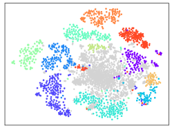
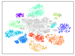
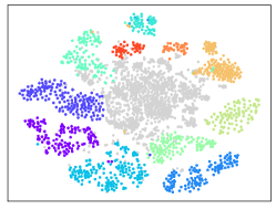
Medium
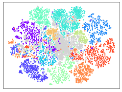
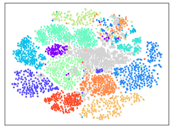
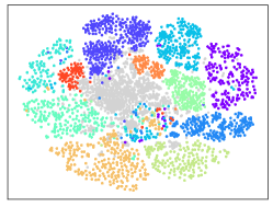
Hard
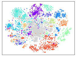
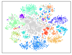
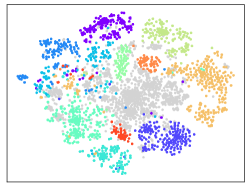
	Resnet101	R50+ViT-B baseline	DToP-R50+ViT-B (ours)

Figure 6: Visualization of revisited Paris ($\mathcal{R}$Paris or $\mathcal{R}$Par) evaluation set under easy, medium and hard protocols [46] (in rows) using t-SNE on output embeddings (12) obtained by different models (in columns) fine-tuned on SfM-120k [48]. For each protocol, positive images are colored by query group label and negative are gray. The set of medium positives is the union of easy and hard positives.

A.5 More visualizations

Figure 6 provides t-SNE visualization of embeddings of $\mathcal{R}$Paris [46] by different models trained on SfM-120k [48]. It is clear that the class distribution of positive images under hard protocol are more overlapping than easy. Medium, being the union of easy and hard, is more populated but classes are better separated than in hard. Vision transformers clearly separate classes better than Resnet101, especially under hard protocol. The difference between our DToP-R50+ViT-B and the baseline hybrid model R50+ViT-B is small.

References

- [1] Artem Babenko and Victor Lempitsky. Aggregating Local Deep Features for Image Retrieval. ICCV, 2015.
- [2] Artem Babenko, Anton Slesarev, Alexandr Chigorin, and Victor Lempitsky. Neural codes for image retrieval. ECCV, 2014.
- [3] Bingyi Cao, André Araujo, and Jack Sim. Unifying deep local and global features for image search. ECCV, 2020.
- [4] Mathilde Caron, Hugo Touvron, Ishan Misra, Hervé Jégou, Julien Mairal, Piotr Bojanowski, and Armand Joulin. Emerging properties in self-supervised vision transformers. ICCV, 2021.
- [5] Chun-Fu Chen, Rameswar Panda, and Quanfu Fan. Regionvit: Regional-to-local attention for vision transformers. arXiv preprint arXiv:2106.02689, 2021.
- [6] Liang-Chieh Chen, George Papandreou, Florian Schroff, and Hartwig Adam. Rethinking atrous convolution for semantic image segmentation. arXiv preprint arXiv:1706.05587, 2017.
- [7] Xiangxiang Chu, Zhi Tian, Yuqing Wang, Bo Zhang, Haibing Ren, Xiaolin Wei, Huaxia Xia, and Chunhua Shen. Twins: Revisiting the design of spatial attention in vision transformers. arXiv preprint arXiv:2104.13840, 2021.
- [8] Xiangxiang Chu, Zhi Tian, Bo Zhang, Xinlong Wang, Xiaolin Wei, Huaxia Xia, and Chunhua Shen. Conditional positional encodings for vision transformers. arXiv preprint arXiv:2102.10882, 2021.
- [9] Stéphane d’Ascoli, Hugo Touvron, Matthew Leavitt, Ari Morcos, Giulio Biroli, and Levent Sagun. Convit: Improving vision transformers with soft convolutional inductive biases. arXiv preprint arXiv:2103.10697, 2021.
- [10] Jia Deng, Wei Dong, Richard Socher, Li-Jia Li, Kai Li, and Li Fei-Fei. Imagenet: A large-scale hierarchical image database. CVPR, 2009.
- [11] Michael Donoser and Horst Bischof. Diffusion processes for retrieval revisited. CVPR, 2013.
- [12] Alaaeldin El-Nouby, Natalia Neverova, Ivan Laptev, and Hervé Jégou. Training vision transformers for image retrieval. arXiv preprint arXiv:2102.05644, 2021.
- [13] Jiemin Fang, Yuzhu Sun, Qian Zhang, Yuan Li, Wenyu Liu, and Xinggang Wang. Densely connected search space for more flexible neural architecture search. CVPR, 2020.
- [14] Socratis Gkelios, Yiannis Boutalis, and Savvas A Chatzichristofis. Investigating the vision transformer model for image retrieval tasks. International Conference on Distributed Computing in Sensor Systems (DCOSS), 2021.
- [15] Chengyue Gong, Dilin Wang, Meng Li, Vikas Chandra, and Qiang Liu. Improve vision transformers training by suppressing over-smoothing. arXiv preprint arXiv:2104.12753, 2021.
- [16] Albert Gordo, Jon Almazan, Jerome Revaud, and Diane Larlus. Deep image retrieval: Learning global representations for image search. ECCV, 2016.
- [17] Benjamin Graham, Alaaeldin El-Nouby, Hugo Touvron, Pierre Stock, Armand Joulin, Hervé Jégou, and Matthijs Douze. Levit: a vision transformer in convnet’s clothing for faster inference. arXiv preprint arXiv:22104.01136, 2021.
- [18] Yinzheng Gu, Chuanpeng Li, and Jinbin Xie. Attention-aware generalized mean pooling for image retrieval. arXiv preprint arXiv:1811.00202, 2018.
- [19] Kai Han, An Xiao, Enhua Wu, Jianyuan Guo, Chunjing Xu, and Yunhe Wang. Transformer in transformer. arXiv preprint arXiv:2103.00112, 2021.
- [20] Jiedong Hao, Jing Dong, Wei Wang, and Tieniu Tan. What is the best practice for cnns applied to visual instance retrieval? ICLR, 2017.
- [21] Bharath Hariharan, Pablo Arbelaez, Ross Girshick, and Jitendra Malik. Hypercolumns for object segmentation and fine-grained localization. 2015.
- [22] Kaiming He, Xinlei Chen, Saining Xie, Yanghao Li, Piotr Dollár, and Ross Girshick. Masked autoencoders are scalable vision learners. arXiv preprint arXiv:2111.06377, 2021.
- [23] Byeongho Heo, Sangdoo Yun, Dongyoon Han, Sanghyuk Chun, Junsuk Choe, and Seong Joon Oh. Rethinking spatial dimensions of vision transformers. arXiv preprint arXiv:2103.16302, 2021.
- [24] Gao Huang, Zhuang Liu, Laurens Van Der Maaten, and Kilian Q Weinberger. Densely connected convolutional networks. CVPR, 2017.
- [25] Matthieu Cord Hugo Touvron, Matthijs Douze, Francisco Massa, Alexandre Sablayrolles, and Hervé Jégou. Training data-efficient image transformers & distillation through attention. arXiv preprint arXiv:2012.12877, 2020.
- [26] Ahmet Iscen, Giorgos Tolias, Yannis Avrithis, Teddy Furon, and Ondrej Chum. Efficient diffusion on region manifolds: Recovering small objects with compact cnn representations. CVPR, 2017.
- [27] Zihang Jiang, Qibin Hou, Li Yuan, Daquan Zhou, Xiaojie Jin, Anran Wang, and Jiashi Feng. Token labeling: Training a 85.5% top-1 accuracy vision transformer with 56m parameters on imagenet. arXiv preprint arXiv:2104.10858, 2021.
- [28] Yannis Kalantidis, Clayton Mellina, and Simon Osindero. Cross-dimensional weighting for aggregated deep convolutional features. ECCV, 2016.
- [29] Alexander Kolesnikov, Alexey Dosovitskiy, Dirk Weissenborn, Georg Heigold, Jakob Uszkoreit, Lucas Beyer, Matthias Minderer, Mostafa Dehghani, Neil Houlsby, Sylvain Gelly, Thomas Unterthiner, and Xiaohua Zhai. An image is worth 16x16 words: Transformers for image recognition at scale. ICLR, 2021.
- [30] Victor Lempitsky and Artem Babenko. Aggregating local deep features for image retrieval. ICCV, 2015.
- [31] Hao Li, Zheng Xu, Gavin Taylor, Christoph Studer, and Tom Goldstein. Visualizing the loss landscape of neural nets. NeurIPS, 2018.
- [32] Yawei Li, Kai Zhang, Jiezhang Cao, Radu Timofte, and Luc Van Gool. Localvit: Bringing locality to vision transformers. arXiv preprint arXiv:2104.05707, 2021.
- [33] Zhaowen Li, Zhiyang Chen, Fan Yang, Wei Li, Yousong Zhu, Chaoyang Zhao, Rui Deng, Liwei Wu, Rui Zhao, Ming Tang, et al. MST: Masked self-supervised transformer for visual representation. NeurIPS, 34, 2021.
- [34] Zeming Li, Chao Peng, Gang Yu, Xiangyu Zhang, Yangdong Deng, and Jian Sun. DetNet: A backbone network for object detection. arXiv preprint arXiv:1804.06215, 2018.
- [35] Tsung-Yi Lin, Piotr Dollár, Ross Girshick, Kaiming He, Bharath Hariharan, and Serge Belongie. Feature pyramid networks for object detection. CVPR, 2017.
- [36] Wei Liu, Dragomir Anguelov, Dumitru Erhan, Christian Szegedy, Scott Reed, Cheng-Yang Fu, and Alexander C Berg. SSD: Single shot multibox detector. ECCV, 2016.
- [37] Ze Liu, Yutong Lin, Yue Cao, Han Hu, Yixuan Wei, Zheng Zhang, Stephen Lin, and Baining Guo. Swin transformer: Hierarchical vision transformer using shifted windows. arXiv preprint arXiv:2103.14030, 2021.
- [38] Sachin Mehta and Mohammad Rastegari. Mobilevit: Light-weight, general-purpose, and mobile-friendly vision transformer. arXiv preprint arXiv:2110.02178, 2021.
- [39] Tony Ng, Vassileios Balntas, Yurun Tian, and Krystian Mikolajczyk. SOLAR: Second-Order Loss and Attention for Image Retrieval. ECCV, 2020.
- [40] Quynh Nguyen, Mahesh Chandra Mukkamala, and Matthias Hein. On the loss landscape of a class of deep neural networks with no bad local valleys. arXiv preprint arXiv:1809.10749, 2018.
- [41] Thao Nguyen, Maithra Raghu, and Simon Kornblith. Do wide and deep networks learn the same things? uncovering how neural network representations vary with width and depth. ICLR, 2021.
- [42] Hyeonwoo Noh, Andre Araujo, Jack Sim, Tobias Weyand, and Bohyung Han. Large-scale image retrieval with attentive deep local features. ICCV, 2017.
- [43] Zhiliang Peng, Wei Huang, Shanzhi Gu, Lingxi Xie, Yaowei Wang, Jianbin Jiao, and Qixiang Ye. Conformer: Local features coupling global representations for visual recognition. arXiv preprint arXiv:2105.03889, 2021.
- [44] James Philbin, Ondrej Chum, Michael Isard, Josef Sivic, and Andrew Zisserman. Object retrieval with large vocabularies and fast spatial matching. CVPR, 2007.
- [45] James Philbin, Ondrej Chum, Michael Isard, Josef Sivic, and Andrew Zisserman. Lost in quantization:Improving particular object retrieval in large scale image databases. CVPR, 2008.
- [46] Filip Radenović, Ahmet Iscen, Giorgos Tolias, Yannis Avrithis, and Ondřej Chum. Revisiting Oxford and Paris: Large-Scale Image Retrieval Benchmarking. CVPR, 2018.
- [47] Filip Radenović, Giorgos Tolias, and Ondřej Chum. CNN image retrieval learns from BoW: Unsupervised fine-tuning with hard examples. ECCV, 2016.
- [48] Filip Radenović, Giorgos Tolias, and Ondřej Chum. Fine-tuning cnn image retrieval with no human annotation. TPAMI, 2019.
- [49] Maithra Raghu, Thomas Unterthiner, Simon Kornblith, Chiyuan Zhang, and Alexey Dosovitskiy. Do vision transformers see like convolutional neural networks? NeurIPS, 34, 2021.
- [50] Olaf Ronneberger, Philipp Fischer, and Thomas Brox. U-net: Convolutional networks for biomedical image segmentation. International Conference on Medical image computing and computer-assisted intervention, 2015.
- [51] Mark Sandler, Andrew Howard, Menglong Zhu, Andrey Zhmoginov, and Liang-Chieh Chen. Mobilenetv2: Inverted residuals and linear bottlenecks. CVPR, 2018.
- [52] Oriane Simeoni, Yannis Avrithis, and Ondréj Chum. Local Features and Visual Words Emerge in Activations. CVPR, 2019.
- [53] Chull Hwan Song, Hye Joo Han, and Yannis Avrithis. All the attention you need: Global-local, spatial-channel attention for image retrieval. WACV, 2022.
- [54] Fuwen Tan, Jiangbo Yuan, and Vicente Ordonez. Instance-level image retrieval using reranking transformers. International Conference on Computer Vision (ICCV), 2021.
- [55] Mingxing Tan, Ruoming Pang, and Quoc V. Le. Efficientdet: Scalable and efficient object detection. CVPR, 2020.
- [56] Giorgos Tolias, Tomas Jenicek, , and Ondréj Chum. Learning and aggregating deep local descriptors for instance-level recognition. ECCV, 2020.
- [57] Ashish Vaswani, Noam Shazeer, Niki Parmar, Jakob Uszkoreit, Llion Jones, Aidan N. Gomez, Lukasz Kaiser, and Illia Polosukhin. Attention is all you need. Advances in Neural Information Processing Systems, 2017.
- [58] Wenhao Wang, Fang Zhao, Shengcai Liao, and Ling Shao. Attentive waveblock: Complementarity-enhanced mutual networks for unsupervised domain adaptation in person re-identification and beyond. Transaction on Image Processing, 2022.
- [59] Weinzaepfel, Philippe and Lucas, Thomas and Larlus, Diane and Kalantidis, Yannis. Learning Super-Features for Image Retrieval. ICLR, 2022.
- [60] Tobias Weyand, Andre Araujo, Bingyi Cao, and Jack Sim. Google Landmarks Dataset v2 - A Large-Scale Benchmark for Instance-Level Recognition and Retrieval. CVPR, 2020.
- [61] Hui Wu, Min Wang, Wengang Zhou, and Houqiang Li. Learning deep local features with multiple dynamic attentions for large-scale image retrieval. ICCV, 2021.
- [62] Haiping Wu, Bin Xiao, Noel Codella, Mengchen Liu, Xiyang Dai, Lu Yuan, and Lei Zhang. Cvt: Introducing convolutions to vision transformers. arXiv preprint arXiv:2103.15808, 2021.
- [63] Fan Yang, Ryota Hinami, Yusuke Matsui, Steven Ly, and Shin’ichi Satoh. Efficient image retrieval via decoupling diffusion into online and offline processing. AAAI, 2019.
- [64] Min Yang, Dongliang He, Miao Fan, Baorong Shi, Xuetong Xue, Fu Li, Errui Ding, and Jizhou Huang. Dolg: Single-stage image retrieval with deep orthogonal fusion of local and global features. ICCV, 2021.
- [65] Shuhei Yokoo, Kohei Ozaki, Edgar Simo-Serra, and Satoshi Iizuka. Two-stage discriminative re-ranking for large-scale landmark retrieval. CVPRW, 2020.
- [66] Kun Yuan, Shaopeng Guo, Ziwei Liu, Aojun Zhou, Fengwei Yu, and Wei Wu. Incorporating convolution designs into visual transformers. ICCV, 2021.
- [67] Li Yuan, Yunpeng Chen, Tao Wang, Weihao Yu, Yujun Shi, Zihang Jiang, Francis EH Tay, Jiashi Feng, and Shuicheng Yan. Tokens-to-token vit: Training vision transformers from scratch on imagenet. arXiv preprint arXiv:2101.11986, 2021.
- [68] Pengchuan Zhang, Xiyang Dai, Jianwei Yang, Bin Xiao, Lu Yuan, Lei Zhang, and Jianfeng Gao. Multi-scale vision longformer: A new vision transformer for high-resolution image encoding. arXiv preprint arXiv:2103.15358, 2021.
- [69] Daquan Zhou, Bingyi Kang, Xiaojie Jin, Linjie Yang, Xiaochen Lian, Zihang Jiang, Qibin Hou, and Jiashi Feng. Deepvit: Towards deeper vision transformer. arXiv preprint arXiv:2103.11886, 2021.
- [70] Jingkai Zhou, Pichao Wang, Fan Wang, Qiong Liu, Hao Li, and Rong Jin. Elsa: Enhanced local self-attention for vision transformer. arXiv preprint arXiv:2112.12786, 2021.
- [71] Ligeng Zhu, Ruizhi Deng, Zhiwei Deng, Greg Mori, and Ping Tan. Sparsely connected convolutional networks. ECCV, 2018.