Abstract: We propose a new fully non-parametric two-step adaptive bandwidth selection method for kernel estimators of spatial point process intensity functions based on the Campbell–Mecke formula and Abramson’s square root law. We present a simulation study to assess its performance relative to the Cronie–Van Lieshout global bandwidth selector and apply the technique to data on induced earthquakes in the Groningen gas field.
AMS Mathematics Subject Classification (2010): 60G55; 60D05; 62M30.
Key words & Phrases: adaptive kernel estimation; bandwidth selection; Campbell–Mecke formula; induced earthquakes; intensity function; point process.

1 Introduction

The first step in any analysis of a spatial point pattern is usually estimating its intensity function (Diggle, 2014; Illian et al., 2008; Van Lieshout, 2019). To do so, various techniques exist. Perhaps the oldest is quadrat counting (DuRietz, 1929) in which one simply reports the number of points falling in each quadrat scaled by the quadrat volume. Instead of fixed quadrats, one might use the cells in a tessellation formed by the pattern itself as the units for counting (Barr & Schoenberg, 2010; Ord, 1978; Schaap & Van de Weygaert, 2000). However, the most popular technique by far seems to be kernel estimation.

The classic kernel estimator for the spatial intensity function Diggle (1985) uses a constant bandwidth. However, intuitively, such a ‘one size fits all’ approach would tend to over-smooth in dense areas, whilst not smoothing enough in sparse regions. As a consequence, finer detail in areas with many points may be lost, whereas the few points in sparser areas might give rise to spurious hot spots. Motivated by similar considerations for density estimation of one-dimensional random variables, Abramson (1982) proposed to use a kernel smoother in which the bandwidth at each observation is weighted by a power of the density at that observation. Doing so reduces the bias significantly (Hall et al., 1995), at least asymptotically.

In kernel estimation, the crucial parameter is the bandwidth. It is often chosen by visual inspection or using a rule of thumb (see e.g. Baddeley et al. (2015, Section 6.5), Illian et al. (2008, Section 3.3) or Scott (1992, Section 6)). Obviously, though, such procedures are rather ad-hoc and subjective.

A different class of techniques is based on asymptotics. For instance for classic kernel estimators, Brook & Marron (1991) considered a Poisson point process on the real line and assumed a simple multiplicative model for the intensity function to derive an asymptotically optimal least-squares cross-validation estimator when the number of points tends to infinity. Lo (2017) picked up the baton and studied the asymptotic (integrated) mean squared error in any dimension without imposing a specific intensity model, again in the regime that the number of points goes to infinity. Van Lieshout (2020) generalised Lo’s work to point processes that may exhibit interaction between the points under the assumption that replicated patterns are available so that infill asymptotics apply. Davies et al. (2018) considered asymptotic expansions for a spatial analogue of the Abramson estimator for Poisson processes as the number of points increases; Van Lieshout (2021) studied infill asymptotics that allow for interaction between the points. It is important to note that the resulting optimal bandwidths depend on the unknown intensity function and cannot be computed in practice without resorting to iterative techniques.

Less subjective yet practical procedures to select a suitable global bandwidth rely on a specific model. For example likelihood cross-validation (Loader, 1999, Section 5.3) assumes the data come from a Poisson point process. Another common approach is to minimise the mean squared error in state estimation for a planar stationary isotropic Cox process (Diggle, 1985). The disadvantage of such techniques is that the underlying assumption may not hold for the pattern at hand, which motivated Cronie & Van Lieshout (2018) to propose a fully non-parametric technique. For adaptive bandwidth selection, to the best of our knowledge, similar procedures do not exist. In this article, we extend the Cronie–Van Lieshout approach to adaptive bandwidth selection and propose a new fully non-parametric, easy to implement, two-step adaptive bandwidth selection method based on the Campbell–Mecke formula that does not require numerical approximation of integrals nor knowledge of second or higher moments.

The plan of this paper is as follows. Section 2 recalls crucial concepts and fixes notation. In Section 3, we discuss adaptive kernel estimators and present the algorithm for selecting the bandwidth. The results of a simulation study into the efficacy of the new approach are given in Section 4.1; an application to a data set concerning induced earthquakes is presented in Section 4.2. The paper closes with a discussion on computational complexity and ideas for future research.

2 Preliminaries and notation

First, let us introduce some notation. Let $\Psi$ be a simple point process (Chiu et al., 2013) in $d$-dimensional Euclidean space ${\mathbb{R}}^{d}$ that is observed in a bounded, non-empty and open subset $W$ of ${\mathbb{R}}^{d}$. We assume that the first order moment measure $\Lambda$ of $\Psi$ defined by

$$\Lambda(A)={\mathbb{E}}\left[\sum_{x\in\Psi}1\{x\in A\}\right],$$

the expected number of points of $\Psi$ that fall in Borel subsets $A$ of ${\mathbb{R}}^{d}$, exists as a locally finite Borel measure and is absolutely continuous with respect to $d$-dimensional Lebesgue measure $\ell$ with a Radon–Nikodym derivative $\lambda:{\mathbb{R}}^{d}\to[0,\infty)$. We will refer to the function $\lambda$ as the intensity function of $\Psi$.

The kernel estimator of the intensity function of a point process was introduced by Diggle (1985) as

$$\widehat{\lambda}(x_{0};h,\Psi,W)=\frac{1}{h^{d}}\sum_{y\in\Psi\cap W}\kappa\left(\frac{x_{0}-y}{h}\right),\quad x_{0}\in W,$$ (1)

possibly divided by a global edge correction factor

$$w(x_{0},h,W)=\frac{1}{h^{d}}\int_{W}\kappa\left(\frac{x_{0}-z}{h}\right)dz.$$

An alternative, local, edge correction can be found in Van Lieshout (2012). The function $\kappa:{\mathbb{R}}^{d}\rightarrow[0,\infty)$ is supposed to be a kernel, that is, a $d$-dimensional probability density function (Silverman, 1986, p. 13) that is even in all its arguments. When $\kappa$ is positive in a neighbourhood of the origin, since $W$ is assumed to be open, the global edge correction factor is non-zero for all $x_{0}\in W$.

The crucial parameter in (1) is the bandwidth $h>0$, which determines the amount of smoothing. For large $h$, the mass of $\kappa$ is spread far and wide, which reduces the variance but may lead to a large bias. For small $h$, the mass of $\kappa$ is concentrated around the observed points of $\Psi\cap W$. Thus, the bias is reduced at the price of a larger variance.

Popular choices of kernel include those belonging to the Beta class (Hall et al., 2004)

$$\kappa^{\gamma}(x)=\frac{\Gamma\left(d/2+\gamma+1\right)}{\pi^{d/2}\Gamma\left(\gamma+1\right)}(1-x^{T}x)^{\gamma}\,1\{x\in B(0,1)\},\quad x\in{\mathbb{R}}^{d},$$ (2)

for $\gamma\geq 0$. Here $B(0,1)$ is the closed unit ball in ${\mathbb{R}}^{d}$ centred at the origin. Note that Beta kernels are supported on the compact unit ball and that their smoothness is governed by the parameter $\gamma$. Indeed, the box kernel defined by $\gamma=0$ is constant and therefore continuous on the interior of the unit ball; the Epanechnikov kernel corresponding to the choice $\gamma=1$ is Lipschitz continuous. For $\gamma>k$ the function $\kappa^{\gamma}$ is $k$ times continuously differentiable on ${\mathbb{R}}^{d}$. An alternative with unbounded support is the Gaussian kernel

$$\kappa(x)=(2\pi)^{-d/2}\exp\left(-x^{T}x/2\right),\quad x\in{\mathbb{R}}^{d}.$$ (3)

Current bandwidth selection techniques are either based on asymptotic expansions (Van Lieshout, 2020) or specific model assumptions (Baddeley et al., 2015; Berman & Diggle, 1989; Loader, 1999) In a recent paper, Cronie & Van Lieshout (2018) proposed a non-parametric alternative based on the Campbell–Mecke formule (Chiu et al., 2013, p. 130) applied to the function $f:{\mathbb{R}}^{d}\to{\mathbb{R}}^{+}$, $f(x)=1\{x\in W\}/\lambda(x)$ known as the Stoyan–Grabarnik statistic (Stoyan & Grabarnik, 1991), which is measurable if $\lambda(x)>0$ for all $x\in W$. Indeed

$${\mathbb{E}}\left\{\sum_{x\in\Psi\cap W}\frac{1}{\lambda(x)}\right\}=\int_{W}\frac{1}{\lambda(x)}\lambda(x)\,\mathrm{d}x=\ell(W).$$ (4)

To select a bandwidth, one may simply replace $\lambda$ by an estimator $\widehat{\lambda}(\cdot;h,\Psi,W)$ in the left hand side of the equation and minimise the discrepancy between $\ell(W)$ and the sum of the $\widehat{\lambda}(x;h,\Psi,W)^{-1}$ over points in $\Psi\cap W$. Formally, set

$$T_{\kappa}(h;\Psi,W)=\left\{\begin{array}[]{ll}\displaystyle\sum_{x\in\Psi\cap W}\frac{1}{\widehat{\lambda}(x;h,\Psi,W)},&\Psi\cap W\neq\emptyset,\\ \ell(W),&\text{ otherwise},\end{array}\right.$$

and choose bandwidth $h>0$ by minimising

$$F_{\kappa}(h;\Psi,W,\ell(W))=\left|T_{\kappa}(h;\Psi,W)-\ell(W)\right|$$ (5)

Since $W$ is assumed to be open and $\kappa(0)>0$ for the kernels considered in this paper, $T_{\kappa}$ and therefore (5) is well-defined with or without edge correction. Moreover, without edge correction, a zero point of the equation (5) exists.

Our goal in the next section is to extend the ideas outlined above to adaptive bandwidths.

3 An adaptive bandwidth selection algorithm

For patterns that contain dense as well as sparse regions, a global ‘one size fits all’ approach to bandwidth selection may not be suitable. Indeed, by definition, it leads to a compromise choice that may be too large for regions that contain many points and too small for regions with few points. The resulting estimator therefore tends to oversmooth and miss fine details in denser regions and contain spurious bumps in the sparser regions. To overcome such problems, in the context of random variables, Abramson (1982) proposed to scale the bandwidth in proportion to a power of the intensity function. In the point pattern setting, a similar adaptive kernel estimator (Davies et al., 2018; Van Lieshout, 2021) is defined as

$$\widehat{\lambda}_{A}(x_{0};h,\Psi,W)=\sum_{y\in\Psi\cap W}\frac{1}{c(y)^{d}h^{d}}\kappa\left(\frac{x_{0}-y}{h\,c(y)}\right)w(y,h,W)^{-1}$$ (6)

where

$$c(y)=\left(\frac{\lambda(y)}{\prod_{z\in\Psi\cap W}\lambda(z)^{1/N(\Psi\cap W)}}\right)^{\alpha},$$ (7)

$N(\Psi\cap W$ denotes the number of points of $\Psi$ that fall in $W$ and $w(y,h,W)$ is an edge correction weight. The power $\alpha$ is set to $-1/2$ when considering asymptotic expansions (Abramson, 1982; Van Lieshout, 2021). In practice, other powers, e.g. $\alpha=-1/d$ when $d\geq 2$, may perform as well.

Let us make a few observations. First, note that points $y$ located in regions with a low intensity are given a larger bandwidth $h\,c(y)$ than those in high intensity regions, as desired. Secondly, we must assume that $\lambda(y)>0$ for each $y\in\Psi\cap W$. The normalisation by the geometric mean is used to obtain a dimensionless quantity for the bandwidth. When focussing on a single point $x_{0}$ (Abramson, 1982; Van Lieshout, 2021), one could normalise simply by $\lambda(x_{0})$. Finally, classic edge correction ideas apply. For example, a local edge correction weight factor in this context takes the form

$$w(y,h,W)=\frac{1}{c(y)^{d}h^{d}}\int_{W}\kappa\left(\frac{z-y}{h\,c(y)}\right)dz$$

and is mass preserving:

$$\int_{W}\widehat{\lambda}_{A}(z;h,\Psi,W)\,dz=N(\Psi\cap W).$$

Since the local bandwidth $h\,c(y)$ depends on the unknown intensity function, (6) cannot be calculated. A common solution is to estimate $c(y)$ by plugging-in a pilot intensity estimator (Chacón & Duong, 2018; Silverman, 1986; Wand & Jones, 1994). For example, one could estimate $\lambda(y)$ by a global bandwidth kernel estimator of the form (1) and set

$$\widehat{c}(y)=\left(\frac{\widehat{\lambda}(y)}{\prod_{z\in\Psi\cap W}\widehat{\lambda}(z)^{1/N(\Psi\cap W)}}\right)^{\alpha}.$$

We propose to use a similar two-step approach to select an adaptive bandwidth. More specifically, first use the Cronie & Van Lieshout technique to select a global bandwidth for the pilot intensity estimator and plug it into (7) to obtain $\widehat{c}(y)$. Then apply (5) to $\widehat{\lambda}_{A}$ with local bandwidths $h\,\widehat{c}(y)$ and optimise over $h$.

More formally, assume that $\Psi\cap W\neq\emptyset$ and let $\kappa$ be some kernel. Then the adaptive bandwidth selection algorithm reads as follows.

Algorithm 1

1.a

Choose a global bandwidth $h_{g}$ by minimising

$$\left|\sum_{x\in\Psi\cap W}\frac{1}{\widehat{\lambda}(x;h,\Psi,W)}-\ell(W)\right|$$

over $h>0$ where, for $x_{0}\in W$,

$$\widehat{\lambda}(x_{0};h,\Psi,W)=\frac{1}{h^{d}}\sum_{y\in\Psi\cap W}\kappa\left(\frac{x_{0}-y}{h}\right).$$

1.b

Calculate a pilot estimator

$$\widehat{\lambda}_{g}(x;h_{g},\Psi,W)=\frac{1}{h_{g}^{d}}\sum_{y\in\Psi\cap W}\kappa\left(\frac{x-y}{h_{g}}\right)w^{-1}(y,h_{g},W)$$

for each $x\in\Psi$, with local edge correction

$$w(y,h_{g},W)=\frac{1}{h_{g}^{d}}\int_{W}\kappa\left(\frac{z-y}{h_{g}}\right)dz.$$

2.a

Choose an adaptive bandwidth $h_{a}$ by minimising

$$\left|\sum_{x\in\Psi\cap W}\frac{1}{\widehat{\lambda}_{A}(x;h,\Psi,W)}-\ell(W)\right|$$

over $h>0$ where, for $x_{0}\in W$,

$$\widehat{\lambda}_{A}(x_{0};h,\Psi,W)=\frac{1}{h^{d}}\sum_{y\in\Psi\cap W}\frac{1}{\widehat{c}(y;h_{g},\Psi,W)^{d}}\kappa\left(\frac{x_{0}-y}{h\,\widehat{c}(y;h_{g},\Psi,W)}\right)$$

with

$$\widehat{c}(y;h_{g},\Psi,W)=\left(\frac{\widehat{\lambda}_{g}(y;h_{g},\Psi,W)}{\prod_{z\in\Psi\cap W}\widehat{\lambda}_{g}(z;h_{g},\Psi,W)^{1/N(\Psi\cap W)}}\right)^{-1/2}.$$

2.b

Apply local edge correction, approximating when necessary, to calculate the final estimator.

In selecting the bandwidth, no edge correction is applied as the clearest optimum is obtained that way (Cronie & Van Lieshout, 2018). Note that to ensure that one never divides by zero, the intensity function estimates must be positive for all $x\in\Psi\cap W$. A sufficient condition is that $\kappa(0)>0$.

Next, we consider the continuity properties of $T_{\kappa}(\cdot;\Psi,W)$ and its limits as the bandwidth approaches zero and infinity. For the global case, (Cronie & Van Lieshout, 2018, Thm 1) guarantees the validity of the first step in the above algorithm. For step [2.a] the following theorem holds.

Theorem 1

Let $\psi$ be a locally finite point pattern of distinct points in ${\mathbb{R}}^{d}$ observed in some non-empty open and bounded window $W$ such that $\psi\cap W\neq\emptyset$. Let $\kappa$ be a Gaussian kernel or a Beta kernel with $\gamma>0$, and $w\equiv 1$. Write $\widehat{\lambda}_{A}$ for the Abramson estimator (6) with

$$c(y;\psi,W)=\left(\frac{1}{\lambda_{p}(y)}\prod_{z\in\psi\cap W}\lambda_{p}(z)^{1/N(\psi\cap W)}\right)^{1/2}$$

for some pilot estimates $\lambda_{p}(y)$ that are strictly positive for all $y\in\psi\cap W$. Then the criterion function

$$T_{\kappa}(h;\psi,W)=\sum_{x\in\psi\cap W}\frac{1}{\widehat{\lambda}_{A}(x;h,\psi,W)}$$

is a continuous function of $h$ on $(0,\infty)$. For the box kernel it is piecewise continuous. In all cases,

$$\lim_{h\to 0}T_{\kappa}(h;\psi,W)=0;\quad\lim_{h\to\infty}T_{\kappa}(h;\psi,W)=\infty.$$

Proof: We will first look at the limit as $h\to 0$. Note that for all $h>0$ and $x\in\psi\cap W$,

$$\widehat{\lambda}_{A}(x;h,\psi,W)\geq\kappa(0)\,c(x;\psi,W)^{-d}h^{-d}>0.$$

Here we use that since the pilot estimator $\lambda_{p}$ is strictly positive on the non-empty pattern $\psi\cap W$, so is $c(\cdot)$. Also, for all kernels considered, $\kappa(0)>0$. Consequently,

$$T_{\kappa}(h;\psi,W)=\sum_{x\in\psi\cap W}\frac{1}{\widehat{\lambda}_{A}(x;h,\psi,W)}\leq\sum_{x\in\psi\cap W}\frac{c(x;\psi,W)^{d}h^{d}}{\kappa(0)}.$$

The right-most expression and therefore $T_{\kappa}(h;\psi,W)$ tends to $0$.

Next let $h\to\infty$. For the box, Beta and Gaussian kernels, $\kappa(\cdot)\leq\kappa(0)$. We already observed that $c(y;\psi,W)$ is strictly positive for $y\in\psi\cap W$ since by assumption $\lambda_{p}$ is. Moreover, it does not depend on $h$ and therefore

$$T_{\kappa}(h;\psi,W) = \sum_{x\in\psi\cap W}\frac{h^{d}}{\sum_{y\in\psi\cap W}c(y;\psi,W)^{-d}\kappa\left(\frac{x-y}{h\,c(y;\psi,W)}\right)}$$

$$\geq h^{d}\sum_{x\in\psi\cap W}\frac{1}{\sum_{y\in\psi\cap W}c(y;\psi,W)^{-d}\kappa(0)}.$$

The right-most expression and therefore $T_{\kappa}(h;\psi,W)$ tends to $\infty$ when $\psi\cap W$ is non-empty.

It remains to look at continuity properties. Both the Beta kernels $\kappa^{\gamma}$ with $\gamma>0$ and the Gaussian kernel are continuous on ${\mathbb{R}}^{d}$. The box kernel is discontinuous on the unit disc $\partial B(0,1)$ only. The function $h\to h^{-d}$ is continuous on $(0,\infty)$. Therefore, for fixed $z\in{\mathbb{R}}^{d}$, the function $h\to\kappa(z/h)$ is also continuous when $\kappa$ is a Gaussian kernel or a Beta kernel with $\gamma>0$. For the box kernel, this function is piecewise continuous, having a discontinuity at $h=||z||$. Observe that, since $\psi\cap W$ is non-empty by assumption, $\kappa(0)>0$ and the pilot estimates $\lambda_{p}(x)$ are strictly positive for every $x\in\psi\cap W$, also the $\widehat{\lambda}_{A}(x;h,\psi,W)$ are strictly positive for $x\in\psi\cap W$ and $h>0$. We conclude that, as a function of $h$ on $(0,\infty)$, $T_{\kappa}(h;\psi,W)$ is continuous for Gaussian kernels and Beta kernels with $\gamma>1$, piecewise continous for the box kernel. $\square$

Theorem 1 implies that Step [2.a] in Algorithm 1 is solvable for $h_{a}$. Usually, but not always, the solution is unique. In case of multiple solutions, one may pick the smallest.

4 Numerical evaluations

In this section we investigate the performance of the proposed local bandwidth selection algorithm for simulated and real-life data.

4.1 Simulation study

constant	trend	high contrast feature
$\lambda_{1}(x,y)\equiv 50$	$\lambda_{3}(x,y)=5+225\,x^{4}$	$\lambda_{7}(x,y)=5+{45\times 50}\times 1_{S}(x,y)/\pi$
$\lambda_{2}(x,y)\equiv 250$	$\lambda_{4}(x,y)=10+200\,x^{4}$	$\lambda_{8}(x,y)=10+{40\times 50}\times 1_{S}(x,y)/\pi$
	$\lambda_{5}(x,y)=25+1125\,x^{4}$	$\lambda_{9}(x,y)=25+{225\times 50}\times 1_{S}(x,y)/\pi$
	$\lambda_{6}(x,y)=50+1000\,x^{4}$	$\lambda_{10}(x,y)=50+{200\times 50}\times 1_{S}(x,y)/\pi$

Table 1: Intensity functions on the unit square. Here $S=\{(x,y)\in[0,1]^{2}:(x-0.5)^{2}+(y-0.6)^{2}<1/100\mbox{ or }(x-0.5)^{2}+(y-0.4)^{2}<1/100\}$.

To compare the performance of the adaptive bandwidth selection approach with the global one, we conduct a simulation study. We consider three types of intensity functions on the unit square in ${\mathbb{R}}^{2}$: a constant intensity, a gradual polynomial trend in the horizontal direction and a central high intensity region contrasting with a low intensity background. Specifically, set

$$\lambda(x,y)=\left\{\begin{array}[]{l}\lambda\\ a+bx^{4}\\ a+b\,1\{(x,y)\in S\}\end{array}\right.$$

for $S=\{(x,y)\in[0,1]^{2}:(x-0.5)^{2}+(y-0.6)^{2}<1/100\mbox{ or }(x-0.5)^{2}+(y-0.4)^{2}<1/100\}$. For each type of function, we set the parameters in such a way that realisations contain approximately $50$ or $250$ points. For the latter two function types, we also vary the fraction $a/b$. Doing so, we obtain the intensity functions summarised in Table 1.

A convenient way to obtain realisations of point processes with spatially varying intensity function $\lambda_{i}$ is to apply independent thinning to a realisations of a stationary point process whose intensity function is known explicitly. Here we choose a Poisson process, a Matérn cluster process and a Matérn hard core process (Matern, 1986). We will need the notation $\bar{\lambda}_{i}=\sup_{(x,y)\in[0,1]^{2}}\lambda_{i}(x,y)$ for the maximal value of $\lambda_{i}$ in $[0,1]^{2}$.

$\lambda$	Poisson	cluster $\nu=5$	cluster $\nu=10$	hard core $\nu=0.9$	hard core $\nu=0.5$
$\lambda_{1}$	10.22	23.17	27.96	10.40	7.73
$\lambda_{2}$	31.76	63.77	82.43	28.37	24.93
$\lambda_{3}$	21.99	33.64	41.34	21.05	20.16
$\lambda_{4}$	16.98	30.51	43.12	16.31	15.00
$\lambda_{5}$	50.57	71.92	102.96	48.62	47.40
$\lambda_{6}$	39.93	72.06	99.85	39.69	35.13
$\lambda_{7}$	562.61	565.66	569.71	561.88	561.03
$\lambda_{8}$	434.81	437.03	441.03	433.15	433.48
$\lambda_{9}$	2,805.35	2,801.78	2,804.41	2,801.64	2,800.81
$\lambda_{10}$	2,164.57	2,165.48	2,176.19	2,174.04	2,143.22

Table 2: Mean integrated squared error relative to expected number of points of kernel estimates over $100$ simulations using a Gaussian kernel with local edge correction and bandwidth chosen by the Cronie–Van Lieshout algorithm for different point process models having intensity functions $\lambda_{i}$, $i=1,\dots,10$.

Poisson process

Let $X$ be a homogeneous Poisson process with intensity function $\bar{\lambda}_{i}$. Then its independent thinning with retention probabilities $\lambda_{i}(x,y)/\bar{\lambda}_{i}$ is a heterogeneous Poisson process with intensity function $\lambda_{i}$.

Matérn cluster process

Let $X_{p}$ be a homogeneous Poisson process with intensity $\kappa$ on $[-0.05,$ $0.05]^{2}$. Assume that each ‘parent’ point $z\in X_{p}$ generates a Poisson number of ‘daughter’ points, say with mean $\nu$ in the closed ball $B(z,0.05)$ of radius $0.05$ around $z$ and write $X$ for the union of daughter points falling in $[0,1]^{2}$. Then $X$ is homogeneous and has constant intensity $\kappa\nu$ on $[0,1]^{2}$. We will consider two degrees of clustering:

• parent intensity $\kappa=\bar{\lambda}_{i}/5$, mean number of daughters $\nu=5$ in a ball of radius $0.05$ around the parent;

• parent intensity $\kappa=\bar{\lambda}_{i}/10$, mean number of daughters $\nu=10$ in a ball of radius $0.05$ around the parent.

In either case, independent thinning with retention probabilities $\lambda_{i}(x,y)/\bar{\lambda}_{i}$ results in a point process $X$ having intensity function $\lambda_{i}$.

Type II Matérn hard core process

Let $X_{g}$ be a homogeneous Poisson process with intensity $\kappa$ on $[-r,r]^{2}$ and assign each ‘ground’ point $z\in X_{g}$ a mark according to the uniform distribution on $(0,1)$ independently of other points. Keep a point $z\in X_{g}\cap[0,1]^{2}$ if no other point of $X_{g}$ with a larger mark lies within distance $r>0$. The resulting point process $X$ is homogeneous and has constant intensity $(1-e^{-\kappa\pi r^{2}})/(\pi r^{2})$ on $[0,1]^{2}$. We will consider two degrees of repulsion:

• ground intensity $\kappa=-10\bar{\lambda}_{i}\log\nu$ with $\nu=0.9$ and hard core distance $r=(10\pi\bar{\lambda}_{i})^{-1/2}$;

• ground intensity $\kappa=-2\bar{\lambda}_{i}\log\nu$ with $\nu=0.5$ and hard core distance $r=(2\pi\bar{\lambda}_{i})^{-1/2}$.

In both cases, independent thinning with retention probabilities $\lambda_{i}(x,y)/\bar{\lambda}_{i}$ results in a point process $X$ having intensity function $\lambda_{i}$.

$\lambda$	Poisson	cluster(5)	cluster(10)	hard core $\nu=0.9$	hard core $\nu=0.5$
$\lambda_{1}$	15.72	40.52	42.99	16.06	11.00
$\lambda_{2}$	52.13	108.20	140.90	47.58	34.67
$\lambda_{3}$	25.58	58.76	81.97	24.96	21.35
$\lambda_{4}$	25.39	77.66	115.98	25.96	19.15
$\lambda_{5}$	90.84	196.21	292.96	81.76	67.02
$\lambda_{6}$	77.80	188.12	289.79	81.04	61.98
$\lambda_{7}$	555.42	554.96	560.86	555.32	555.95
$\lambda_{8}$	401.12	403.04	421.07	396.93	406.10
$\lambda_{9}$	2,663.56	2,586.62	2,545.90	2,606.78	2,535.12
$\lambda_{10}$	1,731.39	1,828.45	1,799.93	1,717.17	1,808.46

Table 3: Mean integrated squared error relative to expected number of points of kernel estimates over $100$ simulations using a Gaussian kernel with local edge correction and bandwidth chosen by Algorithm 1 for different point process models having intensity functions $\lambda_{i}$, $i=1,\dots,10$.

The results of the simulation study are presented in Tables 2 and 3. For each intensity function and each point process model, we generated $100$ simulations in the unit square and calculated the optimal global and adaptive bandwidths using a Gaussian kernel. The tabulated values are the mean integrated squared errors after local edge correction over the $100$ patterns scaled by the exptected number of points. All calculations were done in the R-package spatstat (Baddeley et al., 2015) to which we contributed the function bw.CvL.adaptive.

Comparing Table 2 to Table 3, for homogeneous point processes (intensity functions $\lambda_{1}$ and $\lambda_{2}$) the mean integrated squared error per point is smaller for a global bandwidth. This is not surprising, as all regions are equally rich in points in expectation. When the intensity function is increasing gradually (intensity functions $\lambda_{i}$ for $i=3,\dots,6$) also global bandwidth selection outperforms adaptive bandwidth selection. The situation is reversed when the intensity function shows more distinct features (intensity functions $\lambda_{i}$ for $i=7,\dots,10$). Then, for all point process models considered, local bandwidth selection results in a smaller mean integrated squared error relative to the expected number of points.

4.2 Illustration to pattern of induced earthquakes

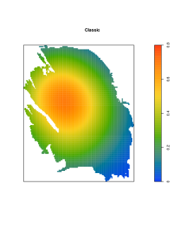
Figure 1: Map of earthquakes of magnitude $M\geq 1.5$ that occurred during the time period 1995–2021 in the Groningen gas field (left-most panel). Kernel estimates of the intensity function using a Gaussian kernel with local edge correction and bandwidth selected by the Cronie–Van Lieshout algorithm (middle panel) and by Algorithm 1 (right-most panel).

In 1959, a large gas field was discovered in Groningen, a province in the north of The Netherlands. Initially, the benefits from the sale of gas were a boon to the Dutch economy. However, from the 1990s earthquakes were being registered in the previously tectonically inactive Groningen region. The pattern of induced earthquakes of magnitude $1.5$ and larger during the period 1995–2021 is depicted in the left-most panel in Figure 1. Note that most earthquakes occurred in the central and western regions.

We applied Algorithm 1 to produce a map of the spatially varying intensity function using a Gaussian kernel and local edge correction. The result is shown in the right-most panel in Figure 1. For comparison, the middle panel shows the estimated kernel estimator upon applying the Cronie–Van Lieshout bandwidth selection algorithm. We conclude that an adaptive approach leads to higher estimated risks in the central gas field, balanced by a lower estimated risk in the periphery.

5 Conclusion

In this article, we introduced a completely non-parametric two-step algorithm for adaptive bandwidth selection for kernel estimators of the spatial intensity function and proved its validity. Simulations showed that for patterns with strong contrasts in point densities, the adaptive kernel estimator outperforms the classic kernel estimator in terms of integrated squared error.

We also demonstrated the feasibility of the proposed algorithm in practice. Given a pilot estimator, the numerical complexity of step [2.a] in Algorithm 1 is of the same magnitude as that of step [1.a]. Indeed, for a pattern with $n$ points, the calculation of $\widehat{\lambda}_{A}$ requires $n$ function evaluations per point. Therefore, calculation of the criterion function $F_{\kappa}$ is quadratic in $n$. Discretising the range of bandwidth values into $n_{h}$ steps, the total computational load is therefore of the order $n_{h}n^{2}$.

Step [2.b] may be computationally demanding, though. For an $M\times N$ grid, equation (6) requires $nMN$ evaluations of the kernel, which may be problematic for large patterns and fine grids. The numerical complexity of calculating the edge correction weights is dependent on the type of edge correction chosen ($nMN$ for local, $M^{2}N^{2}$ for global edge correction). When direct computation is impossible, fast approximation techniques exist (Davies & Baddeley, 2018). Note that for a global bandwidth, direct calculation can be avoided because (1) may be written as a convolution and fast Fourier techniques apply.

Finally, in this article we only considered isotropic kernels. In future, we plan to study adaptive kernel estimators with different bandwidths for the various components.

References

- Abramson (1982) Abramson, I.A. (1982). On bandwidth variation in kernel estimates – A square root law. The Annals of Statistics 10, 1217–1223.
- Baddeley et al. (2015) Baddeley, A., Rubak, E. & Turner, R. (2015). Spatial Point Patterns: Methodology and Applications with R. Boca Raton: CRC Press.
- Barr & Schoenberg (2010) Barr, C.D. & Schoenberg, F.P. (2010). On the Voronoi estimator for the intensity of an inhomogeneous planar Poisson process. Biometrika 97, 977–984.
- Berman & Diggle (1989) Berman, M. & Diggle, P.J. (1989). Estimating weighted integrals of the second-order intensity of a spatial point process. Journal of the Royal Statistical Society: Series B (Statistical Methodology) 51, 81–92.
- Brook & Marron (1991) Brooks, M.M. & Marron, J.S. (1991). Asymptotic optimality of the least-squares cross-validation bandwidth for kernel estimates of intensity functions. Stochastic Processes and their Applications 38, 157–165.
- Chacón & Duong (2018) Chacón, J.E. & Duong, T. (2018). Kernel Smoothing and its Applications. Boca Raton: CRC Press.
- Chiu et al. (2013) Chiu, S.N., Stoyan, D., Kendall, W.S. & Mecke, J. (2013). Stochastic Geometry and its Applications. Chichester: Wiley, 3rd ed.
- Cronie & Van Lieshout (2018) Cronie, O. & Lieshout, M.N.M. van (2018). A non-model based approach to bandwidth selection for kernel estimators of spatial intensity functions. Biometrika 105, 455–462.
- Davies & Baddeley (2018) Davies, T.M. & Baddeley, A. (2018). Fast computation of spatially adaptive kernel estimates. Statistics and Computing 28, 937–956.
- Davies et al. (2018) Davies, T.M., Flynn, C.R. & Hazelton, M.L. (2018). On the utility of asymptotic bandwidth selectors for spatially adaptive kernel density estimation. Statistics and Probability Letters 138, 75–81.
- Diggle (1985) Diggle, P.J. (1985). A kernel method for smoothing point process data. Applied Statistics 34, 138–147.
- Diggle (2014) Diggle, P.J. (2014). Statistical Analysis of Spatial and Spatio-Temporal Point Patterns. Boca Raton: CRC Press, 3rd ed.
- DuRietz (1929) Du Rietz, G.E. (1929). The fundamental units of vegetation. Proceedings of the International Congress of Plant Science 1, 623–627.
- Hall et al. (1995) Hall, P., Hu, T.C. & Marron, J.S. (1995). Improved variable window kernel estimates of probability densities. Annals of Statistics 23, 1–10.
- Hall et al. (2004) Hall, P., Minnotte, M.C. & Zhang, C. (2004). Bump hunting with non-Gaussian kernels. The Annals of Statistics 32, 2124–2141.
- Illian et al. (2008) Illian, J., Penttinen, A., Stoyan, H. & Stoyan, D. (2008). Statistical Analysis and Modelling of Spatial Point Patterns. Chichester: Wiley.
- Van Lieshout (2012) Lieshout, M.N.M. van (2012). On estimation of the intensity function of a point process. Methodology and Computing in Applied Probability 14, 567–578.
- Van Lieshout (2019) Lieshout, M.N.M. van (2019). Theory of Spatial Statistics: A Concise Introduction. Boca Raton: CRC Press.
- Van Lieshout (2020) Lieshout, M.N.M. van (2020). Infill asymptotics and bandwidth selection for kernel estimators of spatial intensity functions. Methodology and Computing in Applied Probability 22, 995–1008.
- Van Lieshout (2021) Lieshout, M.N.M. van (2021). Infill asymptotics for adaptive kernel estimators of spatial intensity functions. Australian and New Zealand Journal of Statistics 63, 159–181.
- Lo (2017) Lo, P.H. (2017). An Iterative Plug-in Algorithm for Optimal Bandwidth Selection in Kernel Intensity Estimation for Spatial Data. Technical University of Kaiserslautern: PhD Thesis.
- Loader (1999) Loader, C. (1999). Local Regression and Likelihood. New York: Springer.
- Matern (1986) Matérn, B. (1986). Spatial variation. Berlin: Springer.
- Ord (1978) Ord, J.K. (1978). How many trees in a forest? Mathematical Sciences 3, 23–33.
- Schaap & Van de Weygaert (2000) Schaap, W.E. & Weygaert, R. van de (2000). Letter to the editor. Continuous fields and discrete samples: Reconstruction through Delaunay tessellations. Astronomy and Astrophysics 363, L29–L32.
- Scott (1992) Scott, D.W. (1992). Multivariate Density Estimation: Theory, Practice and Visualization. New York: Wiley.
- Silverman (1986) Silverman, B.W. (1986). Density Estimation for Statistics and Data Analysis. London: Chapman & Hall.
- Stoyan & Grabarnik (1991) Stoyan, D. & Grabarnik, P. (1991). Second-order characteristics for stochastic structures connected with Gibbs point processes. Mathematische Nachrichten 151, 95–100.
- Wand & Jones (1994) Wand, M.P. & Jones, M.C. (1994). Kernel Smoothing. Boca Raton: Chapman & Hall.