Abstract

This paper is devoted to examining a cosmological model of scale-dependent gravity. The gravitational action is taken to be the Einstein-Hilbert term supplemented with a cosmological constant, where the couplings run with the energy scale. The model is deeply analyzed, confronting its predictions with recent observational data from $H(z)$, $\mu(z)$, and BAO/CMB. The viability of the model is shown, obtaining the best-fit parameters and the maximum likelihood contours for these observables. Finally, a joint analysis is performed.

I Introduction

Current observational evidence shows that we live in a spatially flat Universe dominated by dark matter and dark energy Freedman and Turner (2003). The standard cosmological model ($\Lambda$CDM hereafter) is good enough to give highly accurate predictions of the features of the Cosmic Microwave Background (CMB), primordial abundances of light elements, and large-scale structures. Although we have made significant progress, the nature of the dark sector remains an open question. $\Lambda$CDM is based on General Relativity (GR), a theory consistent with a wealth of observational data from astrophysics and cosmology. However, GR cannot be the ultimate gravity theory since some problems naturally emerge. To mention a few, the theory has the following issues: i) the existence of singularities (suggesting that GR is still incomplete), ii) the non-renormalizability properties, and iii) the fine-tuning problem.

Apart from the issues of GR mentioned above, there are a couple of tensions within the $\Lambda$CDM model itself that have been made clear by the high precision measurements of recent years. The first one to be mentioned is the weak gravitational lensing at low redshifts and the second one the tension between measurements of $H_{0}$ at high red-shift CMB data and low red-shift data (please consult Ryden (2017); Verde et al. (2013); Bolejko (2018); Mörtsell and Dhawan (2018); Abdalla et al. (2022) and references therein). Avoiding the details, the value of the Hubble constant $H_{0}=(67-68)~{}\text{km/(Mpc sec)}$ (extracted by the Planck Collaboration Ade et al. (2016); Aghanim et al. (2020)) is lower than the value found by local measurements, which is $H_{0}=(73-74)~{}\text{km/(Mpc sec)}$ Riess et al. (2016, 2018). There are numerous ways to extend GR and study the cosmological consequences of this extension. A non exhaustive list of such extensions includes i) $f(R)$ theories of gravity Sotiriou and Faraoni (2010); De Felice and Tsujikawa (2010); Hu and Sawicki (2007); Starobinsky (2007) (and refs. Azevedo and Páramos (2016); Pourhassan and Rudra (2020) for a generalized scenario), ii) $f(R,L)$, which basically allows a generalized coupling between curvature and matter, iii) scalar-tensor theories of gravity Brans and Dicke (1961); Brans (1962); Sanchez and Perivolaropoulos (2010) and iv) brane-world models Langlois (2003); Maartens (2004); Dvali et al. (2000). There are further models classified as geometric dark energy such as quintessence Ratra and Peebles (1988), phantom Aref’eva et al. (2006), quintom Lazkoz and Leon (2006), tachyonic Bagla et al. (2003) or k-essence Armendariz-Picon et al. (2001). Recently, the study of cosmological models in which the cosmological constant is assumed to be a function of certain energy scale has attracted attention. The reason is that a time dependent vacuum energy makes possible to resolve the $H_{0}$ problem Poulin et al. (2019) (see also e.g. Basilakos and Solà (2015); Solà et al. (2017); Gómez-Valent and Solà Peracaula (2018); Solà Peracaula (2018) and references therein). The cosmological equations in the most popular $\Lambda$-varying scenarios are generalizations of the Friedmann equations, and they offer a richer phenomenology compared to the $\Lambda$CDM model Öztaş et al. (2018). There are also some works on cosmological models with a variable Newton’s constant, see e.g. Jamil and Debnath (2011); Jamil (2010); Kahya et al. (2015).

The present work focuses on a scale-dependent (SD) gravity model that, when used for cosmology, implies generalized Friedmann equations with time-dependent quantities.

This paper is organized as follows: Section II introduces the framework of the SD gravity model used in this paper. In subsection II.1 we discuss the Null Energy Condition (NEC) to complement the gravitational equations, while subsection II.1 provides the cosmological SD model. Then, in section III, we performed a likelihood analysis using $H(z)$ data (subsection III.1), $\mu(z)$ data (subsection III.2), BAO/CMB data (subsection III.3), and a joint likelihood analysis (subsection III.4). To finish the paper, we summarize our main findings, and provide a short discussion in section IV.

II Framework: the scale-dependent formalism

The effective action $\Gamma[\cdots]$ is a powerful tool commonly used in quantum field theory. It encodes additional quantum features absent in its classical counterpart $I_{0}[\cdots]$. In this formalism the coupling constants of the classical theory become SD quantities i.e.,

$$\{A_{0},B_{0},C_{0},\cdots,Z_{0}\}\ \longrightarrow\ \{A_{k},B_{k},C_{k},\cdots,Z_{k}\},$$ (1)

where the left-hand side corresponds to the classical set and the right-hand side corresponds to the quantum-corrected SD set of couplings. This type of scenario has been proposed and studied in several contexts of gravity, following different methods (please see Weinberg (1976); Hawking and Israel (1979); Wetterich (1993); Morris (1994); Bonanno and Reuter (2000); Reuter and Saueressig (2002); Litim and Pawlowski (2002); Reuter and Weyer (2004); Bonanno and Reuter (2006); Niedermaier (2007); Percacci (2007) and references therein). We will study the effective action

$$\Gamma[g_{\mu\nu},k]=\int\mathrm{d}^{4}x\sqrt{-g}\Bigg{[}\frac{1}{16\pi G_{k}}\Bigl{(}R-2\Lambda_{k}\Bigl{)}\ +\ \mathcal{L}_{M}\Bigg{]},$$ (2)

where $\Lambda_{k}$ and $G_{k}$ are the cosmological and Newton scale–dependent couplings, respectively. A great advantage of working with effective quantum actions like (2) is that they already incorporate the effects of quantum fluctuations. Thus, if a problem is properly addressed in terms of a background solution to this action, no additional quantum corrections need to be added. To obtain background solutions for this effective action one has to derive the corresponding gap equations. Varying the effective action with respect to the inverse metric field, one obtains the corresponding Einstein field equations Reuter and Weyer (2004)

$$G_{\mu\nu}=T_{\mu\nu}^{\text{effec}}=-\Lambda(t)g_{\mu\nu}-{\Delta t}_{\mu\nu},$$ (3)

where

$${\Delta t}_{\mu\nu}=G(t)\Bigl{[}g_{\mu\nu}\nabla^{\alpha}\nabla_{\alpha}-\nabla_{\mu}\nabla_{\nu}\Bigl{]}G(t)^{-1}.$$ (4)

To get physical information out of those equations one has to set the renormalization scale in terms of the physical variables of the system under consideration $k\rightarrow k(x,\dots)$. However, the connection between $k$ and the system’s physical variables is not uniquely defined. Thus, if one selects a particular relation between $k$ and $\{t,r,\theta,\phi\}$, one introduces a source of uncertainties to be considered. Thus, whether one wishes to bypass such a disadvantage, one then should close the system following an alternative way. This can for example be achieved by taking variations with respect to the renormalization scale, i.e.,

$$\frac{\mathrm{d}\Gamma[g_{\mu\nu},k]}{\mathrm{d}k}\Bigg{|}_{k=k_{\text{opt}}}=0$$ (5)

Albeit possible, the implementation of such an equation turns out to be cumbersome. Finally, to supplement our system of equations and solve the system in a consistent way, one can use the contraction $T^{\text{effec}}_{\mu\nu}\ell^{\mu}\ell^{\nu}=0$ (for radial null vectors) as closure condition. In the next section we will briefly elaborate on such an alternative closure condition.

II.1 SD gravity with a null energy condition

Energy conditions play an essential role in many applications of general relativity, from cosmology to black-hole physics, and their importance in formulating singularity theorems. These energy conditions consist of restrictions on the stress-energy tensor. Their purpose is three-fold. Firstly, energy conditions allow us to get a sense of ”normal matter” since they capture standard features of a different kind of matter. Secondly, all the properties of matter fields are contained the Einstein’s equations and many of their modifications (including the present work) through the stress-energy tensor. Therefore, one can analyze the resulting dynamical system without recurring to the complex behavior of the field content of the theory. Thirdly, energy conditions enable a conceptual simplification for bypassing complicated computation, as shown in the singularity theorems Penrose (1965); Hawking (1966)

This last point is one of the strongest criticisms about the range of validity of the energy conditions. Pointwise energy conditions on the stress-energy tensor are generally considered as over-simplification that are not able to capture all the features of the systems under scrutiny. An example is their application to quantum fields, where the violation of all pointwise energy conditions motivates the introduction of the quantum energy inequalities Ford and Roman (1995); Fewster (2012), which allows a finite, possibly negative, lower bound. An intermediate step consists in the averaged energy conditions that average the components of the stress-energy tensor along suitable causal curves while preserving lower bounds to zero. It is noteworthiness to remark that the validity of the energy conditions strongly depends on the contributions to the total stress-energy tensor.

SD gravity with a pointwise NEC has been used on: i) cosmology Canales et al. (2020); Alvarez et al. (2021, 2022); Panotopoulos and Rincón (2021); Bargueño et al. (2021), ii) relativistic stars Panotopoulos et al. (2021, 2020) and iii) black holes Koch and Rioseco (2016); Koch et al. (2016); Rincón and Koch (2018); Rincón et al. (2017); Contreras et al. (2017). In this manuscript, we will continue the ideas presented in Canales et al. (2020); Alvarez et al. (2021, 2022), with the inclusion of the pointwise NEC together with the modified Friedmann equations for the SD scenario of Einstein gravity with minimally coupled matter. The idea is the following. Given an observer on a null geodesic, the effective stress-energy tensor $\kappa_{k}\,T^{\text{eff}}_{\mu\nu}\equiv\kappa_{k}\,T_{\mu\nu}-\Delta t_{\mu\nu}$ must follow $T^{\text{eff}}_{\mu\nu}\,k^{\mu}k^{\nu}\geq 0$ Canales et al. (2020). As discussed in Alvarez et al. (2021), the NEC is independent of the SD cosmological constant; thus, it dictates the evolution of Newton’s coupling through different energy scales. Values lower than zero are forbidden at a point Tipler (1978); Kontou and Sanders (2020), while values greater than zero falls into non-physical scenarios with negative values of the Newton constant at early or late evolution time Alvarez et al. (2021). Therefore, the saturated energy condition $\Delta t_{\mu\nu}\,k^{\mu}\,k^{\nu}=0$ seems to be well-justified. One can see the advantage of demanding the NEC for the whole $T^{\text{eff}}_{\mu\nu}$ instead of just $T_{\mu\nu}$ by looking at its geometrical counterpart: if the NEC is applied to $T^{\text{eff}}_{\mu\nu}$ and $\Delta t_{\mu\nu}$ fulfills the saturated NEC, it implies $R_{\mu\nu}\,k^{\mu}k^{\nu}\geq 0$, which means that non-rotating null geodesic congruence locally converges, ensuring that gravity is attractive for massless particles Kontou and Sanders (2020)

To evaluate the validity of the inclusion of a (saturated) energy condition for closing the system of equation, one has to compare the theoretical result with physical observables. In this sense, a first step was taken in Alvarez et al. (2021), where the tension between early and late-time measurements of $H_{0}$ was studied for the scale-dependence correction of the classical $\Lambda$CDM model. In the present work, the idea is being put on the edge by confronting our theoretical model with the latest Type Ia Supernova (SN Ia), Baryon Acoustic Oscillations (BAO), and CMB radiation observations.

II.2 The cosmological SD model

In what follows, we will summarize the main ingredients and the differential equations which describe the cosmological background evolution of a SD FLRW Universe which is subject to a null energy condition in the gravitational sector Alvarez et al. (2021).

Thus, rewritten the original equations to a more convenient set, we then have

$$\frac{1}{H_{0}^{2}}\left(H^{2}-H\frac{\dot{g}}{g}\right)=\Omega_{\Lambda}\lambda(t)+\frac{\Omega_{r}}{a^{4}}g+\frac{\Omega_{m}}{a^{3}}g\,,$$ (6)

$$\frac{1}{H_{0}^{2}}\left(2\dot{H}+3H^{2}-2H\frac{\dot{g}}{g}+2\frac{\dot{g}^{2}}{g^{2}}-\frac{\ddot{g}}{g}\right)=3\Omega_{\Lambda}\lambda(t)-\frac{\Omega_{r}}{a^{4}}g\,,$$ (7)

$$\frac{\ddot{g}}{g}-H\frac{\dot{g}}{g}-2\frac{\dot{g}^{2}}{g^{2}}=0\,,$$ (8)

where $g(t)$ and $\lambda(t)$ are defined by

$$g(t)\equiv\frac{G(t)}{G_{0}}\,,\hskip 28.45274pt\lambda(t)\equiv\frac{\Lambda(t)}{\Lambda_{0}}\,.$$ (9)

As in the $\Lambda$CDM model, the density parameters $\Omega_{m}$, $\Omega_{r}$, and $\Omega_{\Lambda}$ describe the contents of the Universe. The time dependence of the $\Lambda$ coupling that is implied in the scale–dependent scenario results in time-dependent dark energy density

$$\Omega_{\Lambda}\lambda(t)=\frac{\Lambda(t)}{3H_{0}^{2}}\,.$$ (10)

The value of $\Omega_{\Lambda}\lambda(t)$ is not independent, since it can be expressed as the present values of the functions and parameters from (6) or (7).

We will explore the phase space of the dynamical system given by Eqs. (6-8). For this discussion, it is convenient to use the dimensionless functions (9) and

$$x=\frac{a(t)}{a_{0}}\,.$$ (11)

The SD cosmological equations take the form

$$\frac{x^{\prime}(\tau)^{2}}{x(\tau)^{2}}-\frac{g^{\prime}(\tau)x^{\prime}(\tau)}{g(\tau)x(\tau)}=\Omega_{m}g(\tau)x(\tau)^{-3}+\Omega_{r}g(\tau)x(\tau)^{-4}+\Omega_{\Lambda}\lambda(\tau)\,,$$ (12)

$$\frac{x^{\prime}(\tau)^{2}}{x(\tau)^{2}}-2\frac{g^{\prime}(\tau)x^{\prime}(\tau)}{g(\tau)x(\tau)}+2\frac{g^{\prime}(\tau)^{2}}{g(\tau)^{2}}+2\frac{x^{\prime\prime}(\tau)}{x(\tau)}-\frac{g^{\prime\prime}(\tau)}{g(\tau)}=-\Omega_{r}g(\tau)x(\tau)^{-4}+3\Omega_{\Lambda}\lambda(\tau)\,,$$ (13)

$$\frac{g^{\prime\prime}(\tau)}{g(\tau)}-\frac{g^{\prime}(\tau)x^{\prime}(\tau)}{g(\tau)x(\tau)}-2\frac{g^{\prime}(\tau)^{2}}{g(\tau)^{2}}=0\,.$$ (14)

The evolution of this dynamical system can be determined by giving the initial conditions $x(\tau_{0})$, $x^{\prime}(\tau_{0})$, $g(\tau_{0})$ and $g^{\prime}(\tau_{0})$, where we denoted $\tau_{0}$ as the present value of the evolution coordinate $\tau$.

When switching between the time variables $t$ and $\tau$ is useful to have at hand the relations,

$$\dot{x}(t)/x(t)= (H_{100}h)x^{\prime}(\tau)/x(\tau)\,,$$ (15)

$$t= (H_{100}h)^{-1}\tau\,.$$ (16)

where $H_{100}=100\text{ km}\text{ s}^{-1}\text{ Mpc}^{-1}$.

The parameter $h$ will be one of the phenomenological parameters of our model. A particular cosmological model is defined by giving the values of two input parameters at the level of the action $\Omega_{m}$, $\Omega_{r}$ and four initial conditions $x(\tau_{0})$, $x^{\prime}(\tau_{0})$, $g(\tau_{0})$ and $g^{\prime}(\tau_{0})$. For the subsequent analysis it is conventient to work with the parameters $\alpha\equiv x^{\prime}(\tau_{0})/x(\tau_{0})$ and the time-rescaling parameter $h$.

III Observational constraints

We do not know analytical solutions of (12) – (14) under generic initial data and density parameters and therefore we will use numerical solutions. Based on the results of Alvarez et al. (2022), we integrate the equations numerically.

III.1 Constraints from $H(z)$ data

We can use the expressions for the redshift and the Hubble parameter,

$$z= \frac{x_{0}}{x(\tau)}-1\,,$$ (17)

$$H= hH_{100}\frac{x^{\prime}(\tau)}{x(\tau)}\,.$$ (18)

in terms of the numerical solution $x(\tau)$. The subscript 0 represents present day values and, from (11), we see that it is sufficient to consider models with $x_{0}=1$.

We used the latest $H(z)$ data, consisting in 28+1 data points given in Rani et al. (2015). This dataset is based in 28 points given in Farooq and Ratra (2013) plus the value of $H_{0}$ estimated in Riess et al. (2011). To perform the likelihood analysis we define $\chi_{H}^{2}$ as

$$\chi_{H}^{2}(\theta)=\sum_{i=1}^{29}\left(\frac{H(z_{i};\theta)-H^{\text{obs}}_{i}}{\sigma_{i}}\right)^{2}\,.$$ (19)

Here, $H(z_{i};\theta)$ represent model predictions for a given set of parameters and $H^{\text{obs}}_{i}$ represent the observational data points which are known with the uncertainty $\sigma_{i}$.

In this paper we will consider two main models within the framework of the SD cosmology,

$$\theta_{\text{model A}}= (x^{\prime}_{0},\ g^{\prime}_{0},\ \Omega_{m}),\quad\quad\;\,\text{with }x_{0}=1,\ g_{0}=\ 1,\ \Omega_{r}=0,\,h=0.682\,,$$ (20)

$$\theta_{\text{model B}}= (x^{\prime}_{0},\ g^{\prime}_{0},\ h,\ \Omega_{m}),\quad\text{with }x_{0}=\ 1,\ g_{0}=1,\ \Omega_{r}=0\,.$$ (21)

We determined best fit parameters (BF) by minimizing $\chi_{H}^{2}(\theta)$. In the case of model A we obtained the results $x^{\prime}(0)\approx 1.053$, $g^{\prime}(0)\approx-1.139$ and $\Omega_{m}=0.262$, with a value of $\chi_{H}^{2}(\theta_{\text{BF}})\approx 18.779$ and a reduced chi-squared $\chi_{H}^{2}(\theta_{\text{BF}})/\nu\approx 0.722$, where $\nu$ is the number of degrees of freedom, $\nu(H(z))=26$ (a value $\chi^{2}/\nu$ around 1 shows accordance between observations and error variance). In the case of model B we obtained the results $x^{\prime}(0)\approx 1.346$, $g^{\prime}(0)\approx-1.398$, $h=0.534$ and $\Omega_{m}\approx 0.436$, with a value of $\chi_{H}^{2}(\theta_{\text{BF}})\approx 18.951$ and a reduced chi-squared $\chi_{H}^{2}(\theta_{\text{BF}})/\nu\approx 0.758$, where $\nu$ is the number of degrees of freedom, $\nu(H(z))=25$. The derived values for $H_{0}$ are $H_{0}\equiv h\cdot H_{100}\cdot x^{\prime}(0)\approx 71.81\text{ km}\text{ s}^{-1}\text{ Mpc}^{-1}$ for model A and $H_{0}\approx 71.3\text{ km}\text{ s}^{-1}\text{ Mpc}^{-1}$ for model B.

For the computation of maximum likelihood contours (M.L.C.) we implemented random sampling with a Markov chain Monte Carlo ensemble sampler using the EMCEE Python library Foreman-Mackey et al. (2013). We used uniform priors, and for our sampling, we used 200 walkers, 400,000 sampling steps and we discarded a few times the autocorrelation time for burn-in. We averaged over a fraction of the autocorrelation time. For model A, we obtain the results of figure 2, while for model B, the results are shown in figure 3. In the figures, we show contour levels at 68% and 95%. We repeated this procedure for the other observables considered in this paper.

From the M.L.C. we can see that the $H(z)$ data is very good at constraining model A. For model B there is degeneracy within parameters and the contours are less restrictive.

III.2 Constraints from $\mu(z)$ data

The observations of type Ia supernovae (SNe Ia) directly measure the apparent magnitude $m$ of supernovae and their redshift $z$. The apparent magnitude is related to the luminosity distance $d_{L}$ of the supernova through

$$m=M+5\log_{10}\left(\frac{d_{L}(z)}{1\text{ Mpc}}\right)+25\,,$$ (22)

where $M$ is the absolute magnitude, which is considered to be constant for all SNe Ia. It is convenient to use the Hubble free luminosity distance,

$$D_{L}(z)=\frac{H_{0}}{c}d_{L}(z)\,,$$ (23)

and the distance modulus $\mu(z)$,

$$\mu\equiv m-M=5\log_{10}\left(\frac{D_{L}(z)}{H_{0}}\right)+52.38\,.$$ (24)

The Hubble free luminosity distance $D_{L}(z)$ is determined using

$$\frac{D_{L}(z)}{H_{0}}=(1+z)\int_{0}^{z}\frac{dz^{\prime}}{H(z^{\prime})}\,,$$ (25)

where we compute $z$ and $H(z)$ using (17) and (18).

We used the Union 2.1 $\mu(z)$ data compilation that consists of data for 833 SNe, drawn from 19 datasets. Of these, 580 SNe pass usability cuts Suzuki et al. (2012), which are publicly available.

We define $\chi^{2}_{\mu}$ as

$$\chi_{\mu}^{2}(\theta)=\sum_{i,j=1}^{580}X_{i}(C^{-1})_{i,j}X_{j}\,,\qquad X_{i}=\mu(z_{i};\theta)-\mu^{\text{obs}}_{i},$$ (26)

where $\mu(z;\theta)$ represents model predictions for a given set of parameters and $C$ is the full covariance matrix. We determined best fit parameters by minimizing $\chi^{2}_{\mu}(\theta)$. In the case of model A we obtained the results $x^{\prime}(0)\approx 1.018$, $g^{\prime}(0)\approx-1.073$ and $\Omega_{m}=0.334$, with a value of $\chi_{\mu}^{2}(\theta_{\text{BF}})\approx 545.170$ and a reduced chi-squared $\chi_{\mu}^{2}(\theta_{\text{BF}})/\nu\approx 0.945$, where $\nu$ is the number of degrees of freedom, $\nu(\mu(z))=577$. In the case of model B we obtained the results $x^{\prime}(0)\approx 1.251$, $g^{\prime}(0)\approx-1.329$, $h=0.555$ and $\Omega_{m}\approx 0.509$, with a value of $\chi_{\mu}^{2}(\theta_{\text{BF}})\approx 545.171$ and a reduced chi-squared $\chi_{\mu}^{2}(\theta_{\text{BF}})/\nu\approx 0.946$, where $\nu$ is the number of degrees of freedom, $\nu(\mu(z))=576$. The derived values for $H_{0}$ are $H_{0}\approx 69.43\text{ km}\text{ s}^{-1}\text{ Mpc}^{-1}$ for model A and $H_{0}\approx 69.43\text{ km}\text{ s}^{-1}\text{ Mpc}^{-1}$ for model B.

From the M.L.C. we can see that the $\mu(z)$ data is very good at constraining $x^{\prime}(0)$, but there is a large degeneracy in $g^{\prime}(0)$. Model B also suffers from a large degeneracy in $h$. This degeneracy in $h$ is the reason why the variation of this parameter in model B did not lead to an improvement of the reduced $\chi^{2}$ with respect to model A.

III.3 Constraints from BAO/CMB data

We can look for the paramater space of the scale dependent model that is favoured by the BAO from low-redshift data. The BAO scale is set by the radius of the sound horizon at the end of the drag epoch $z_{d}$, when photon pressure is no longer able to avoid gravitational instability of the baryons,

$$r_{s}=\int_{z_{d}}^{\infty}\frac{c_{s}(z)}{H(z)}dz\,,$$ (27)

where the speed of sound in the photon-baryon fluid is

$$c_{s}(z)=3^{-1/2}c{(1+3/4\rho_{b}(z)/\rho_{\gamma}(z))}^{-1/2}\,.$$ (28)

A precise prediction of the BAO signal requires a full Boltzmann code computation, but for reasonable variations about a fiducial model, in many cases, the ratio of BAO scales is computed by the ratio of $r_{s}$ values computed from the integral (27), see for instance Aubourg et al. (2015). This often imposes a prior of the CMB measurement from the Planck satellite. We will compute (27) assuming dynamics from the full SD equations for $H(z)$ in (27). However, in the absence of the existence of a full Boltzmann study of the CMB properties within the SD cosmology, we will use the Planck values Aghanim et al. (2020) of the parameters in (28) as priors. This setup works reasonably well under the assumption that $\dot{g}_{0}$ is small enough, and therefore the $\Lambda$CDM predictions are close enough to the set of predictions of the SD model.

The angular diameter distance $D_{A}$ and the volume-averaged scale $D_{V}$ are related to $H(z)$ by Eisenstein et al. (2005)

$$D_{A}(z)= \frac{1}{1+z}\int_{0}^{z}\frac{dz^{\prime}}{H(z^{\prime})}\,,$$ (29)

$$D_{V}(z)= \left((1+z)^{2}D_{A}^{2}(z)\frac{z}{H(z)}\right)^{1/3}.$$ (30)

We used the dataset compiled by Giostri et al for the observable $r_{s}(z_{d})/D_{V}(z)$ Giostri et al. (2012) that comprises: two points at $z=0.2$ and $z=0.35$ extracted from Percival et al Percival et al. (2010), a point at $z=0.106$ extracted from the 6dF Galaxy Survey Beutler et al. (2011), and three points at $z=0.44$, $z=0.60$ and $z=0.73$ extracted from the BAO results by the WiggleZ team Blake et al. (2011).

We define $\chi_{\text{BAO}}^{2}$ as

$$\chi_{\text{BAO}}^{2}(\theta)=\sum_{i,j=1}^{6}X_{i}(C^{-1})_{ij}X_{j}\,,\qquad X_{i}=(r_{s}(z_{d};\theta)/D_{V}(z_{i};\theta))-(r_{s}(z_{d})/D_{V})^{\text{obs}}_{i}$$ (31)

where $(r_{s}(z_{d};\theta)/D_{V}(z_{i};\theta))$ represents model predictions for a given set of parameters and $C$ is the covariance matrix Giostri et al. (2012). We determined best fit parameters by minimizing $\chi^{2}_{BA0}(\theta)$. In the case of model A we obtained the results $x^{\prime}(0)\approx 0.479$, $g^{\prime}(0)\approx 0.408$ and $\Omega_{m}=0.080$, with a value of $\chi_{\text{BAO}}^{2}(\theta_{\text{BF}})\approx 2.159$ and a reduced chi-squared $\chi_{\text{BAO}}^{2}(\theta_{\text{BF}})/\nu\approx 0.720$, where $\nu$ is the number of degrees of freedom, $\nu(\mu(z))=3$. In the case of model B we obtained the results $x^{\prime}(0)\approx 0.901$, $g^{\prime}(0)\approx 0.768$, $h=0.363$ and $\Omega_{m}\approx 0.282$, with a value of $\chi_{\text{BAO}}^{2}(\theta_{\text{BF}})\approx 2.159$ and a reduced chi-squared $\chi_{\text{BAO}}^{2}(\theta_{\text{BF}})/\nu\approx 1.080$. The derived values for $H_{0}$ are $H_{0}\approx 32.67\text{ km}\text{ s}^{-1}\text{ Mpc}^{-1}$ for model A and $H_{0}\approx 32.71\text{ km}\text{ s}^{-1}\text{ Mpc}^{-1}$ for model B. As it can be seen from the M.L.C. of figures 2 and 3, there is large degeneracy for BAO within the SD model. This means that the BAO data is not as well suited as the other observational data sets, to constrain the parameters of the model.

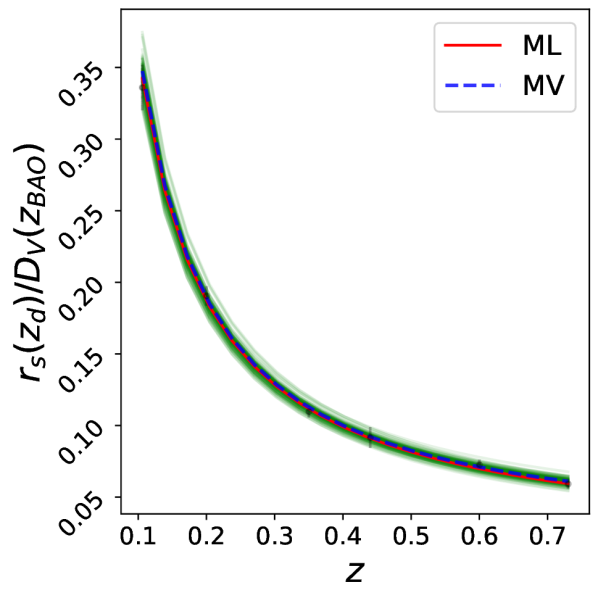
(a) Model A, where the parameter $h=0.682$.

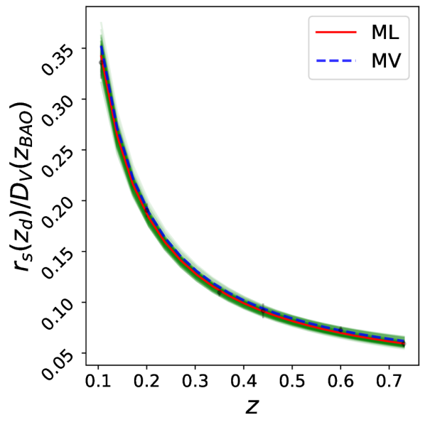
(b) Model B.

Figure 1: Red is the BF value (ML) and blue-dashed the mean value (MV). In green are the predictions for a hundred randomly selected set of parameters within the posterior distribution.

III.4 Joint analysis

In this subsection we present the results of a joint analysis of the previously presented separate results for $H(\theta)$, $\mu(z,\theta)$, and $X_{i}(\theta)$. For this purpose the results are summarized in table 1.

		$H(z)$	$\mu(z)$	BAO	Joint
model A	$x^{\prime}(0)$	1.053	1.018	0.479	1.025
	$g^{\prime}(0)$	-1.139	-1.073	0.408	-0.847
	$\Omega_{\text{mat}}$	0.262	0.334	0.080	0.323
	$\chi^{2}/\nu$	0.722	0.945	0.720	0.928
model B	$x^{\prime}(0)$	1.346	1.251	0.901	1.043
	$g^{\prime}(0)$	-1.398	-1.329	0.768	-0.861
	$h$	0.534	0.555	0.363	0.670
	$\Omega_{\text{mat}}$	0.436	0.509	0.282	0.335
	$\chi^{2}/\nu$	0.758	0.946	1.080	0.930

Table 1: Summary of the best fit values obtained in this paper.

More detailed information on the result of the joint analysis is shown in the corner plots 2 and 3. These corner plots of M.L.C. show that the three observables are compatible within the SD cosmological model therefore we will consider the joint analysis. We will assume that the observables are effectively independent by defining the combined $\chi_{\text{joint}}^{2}$ value as

$$\chi^{2}_{\text{joint}}=\chi^{2}_{H}+\chi^{2}_{\mu}+\chi^{2}_{\text{BAO}}\,.$$ (32)

In the case of model A we obtained the results $x^{\prime}(0)\approx 1.025$, $g^{\prime}(0)\approx-0.847$ and $\Omega_{m}=0.323$, with a value of $\chi_{\text{joint}}^{2}(\theta_{\text{BF}})\approx 568.159$ and a reduced chi-squared $\chi_{\text{joint}}^{2}(\theta_{\text{BF}})/\nu\approx 0.928$, where $\nu$ is the number of degrees of freedom, $\nu(\mu(z))=612$. In the case of model B we obtained the results $x^{\prime}(0)\approx 1.043$, $g^{\prime}(0)\approx-0.861$, $h=0.670$ and $\Omega_{m}\approx 0.335$, with a value of $\chi_{\text{joint}}^{2}(\theta_{\text{BF}})\approx 568.159$ and a reduced chi-squared $\chi_{\text{joint}}^{2}(\theta_{\text{BF}})/\nu\approx 0.930$, where $\nu$ is the number of degrees of freedom, $\nu(\mu(z))=611$. The derived values for $H_{0}$ are $H_{0}\approx 69.91\text{ km}\text{ s}^{-1}\text{ Mpc}^{-1}$ for model A and $H_{0}\approx 69.88\text{ km}\text{ s}^{-1}\text{ Mpc}^{-1}$ for model B.

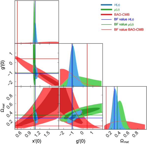
(a) .

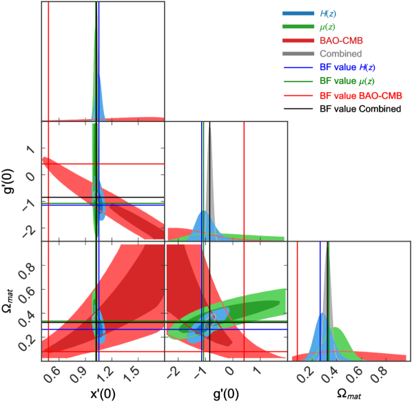
(b) .

Figure 2: Model A, where the parameter $h=0.682$. Corner plots showing the 1D marginalized and 2D joint posterior distributions.

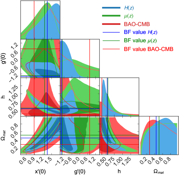
(a) .

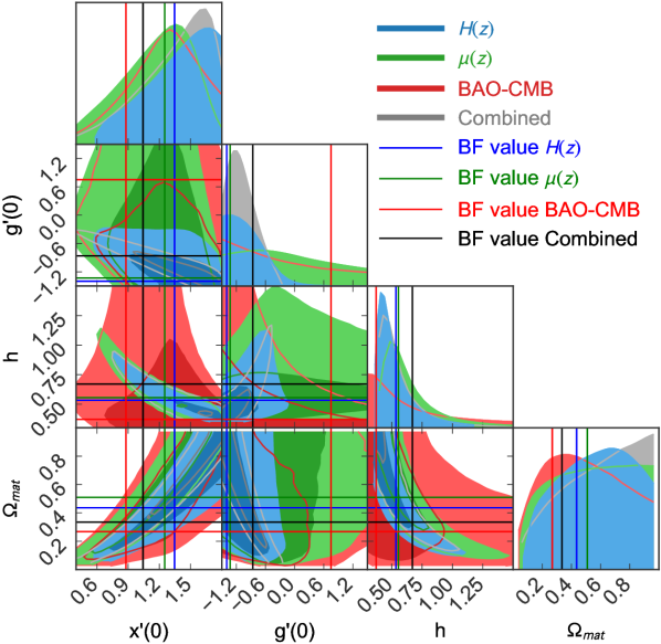
(b) .

Figure 3: Model B. Corner plots showing the 1D marginalized and 2D joint posterior distributions.

IV Discussion and conclusion

In previous papers we considered the SD cosmological model as a viable solution for the $H_{0}$ problem Alvarez et al. (2021). In Alvarez et al. (2022) we also studied the statefinder parameters of the SD model and in particular we showed that the dynamics predicted by the SD model is not equivalent to the dynamics of BD. In the present paper we performed a likelihood analysis of benchmarks of the SD model, were we allowed for three and four parameters to vary respectively. We used three observables to obtain best-fit values and the maximum likelihood contours. We checked compatibility of the observables and also performed the joint analysis. Our present analysis is fundamental in understanding the physically relevant values of the parameters of the SD model.

There are future refinements that can be made to our study. With respect to the sound horizon $r_{d}$ that is used as the standard ruler to calibrate the BAO observations Heavens et al. (2014); Verde et al. (2017), and following the ideas of Zhang and Huang (2021), it is interesting to carry out a full measurement of the parameters of the SD cosmological model and the scale of the BAO from low-redshift data. It would be also interesting to implement a full Boltzmann equation solver to obtain CMB-SD predicted parameters from the CMB features only. For the sake of simplicity, in the present model we have assumed flat spatial geometry but it would be interesting to study the implications of spatial curvature in the context of the SD model.

In summary, our analysis shows, that the presented SD model is in very good agreement with the observational data sets Farooq and Ratra (2013); Riess et al. (2011); Suzuki et al. (2012); Giostri et al. (2012). This is proven by analyzing these data sets separately and in a joint analysis. One of the most striking features of our combined analysis is that, if one allows for scale-dependence, the data supports clearly a non-vanishing time derivative of the gravitational coupling of the order of $g^{\prime}(0)\approx-1$.

Acknowlegements

A.R. is funded by the María Zambrano contract ZAMBRANO 21-25 (Spain). P. A. acknowledges MINEDUC-UA project ANT 1755 and Semillero de Investigación project SEM18-02 from Universidad de Antofagasta, Chile.

References

- Freedman and Turner (2003) W. L. Freedman and M. S. Turner, Rev. Mod. Phys. 75, 1433 (2003), eprint astro-ph/0308418.
- Ryden (2017) B. Ryden, Nature Phys. 13, 314 (2017).
- Verde et al. (2013) L. Verde, P. Protopapas, and R. Jimenez, Phys. Dark Univ. 2, 166 (2013), eprint 1306.6766.
- Bolejko (2018) K. Bolejko, Phys. Rev. D 97, 103529 (2018), eprint 1712.02967.
- Mörtsell and Dhawan (2018) E. Mörtsell and S. Dhawan, JCAP 09, 025 (2018), eprint 1801.07260.
- Abdalla et al. (2022) E. Abdalla et al., JHEAp 34, 49 (2022), eprint 2203.06142.
- Ade et al. (2016) P. A. R. Ade et al. (Planck), Astron. Astrophys. 594, A13 (2016), eprint 1502.01589.
- Aghanim et al. (2020) N. Aghanim et al. (Planck), Astron. Astrophys. 641, A6 (2020), [Erratum: Astron.Astrophys. 652, C4 (2021)], eprint 1807.06209.
- Riess et al. (2016) A. G. Riess et al., Astrophys. J. 826, 56 (2016), eprint 1604.01424.
- Riess et al. (2018) A. G. Riess et al., Astrophys. J. 861, 126 (2018), eprint 1804.10655.
- Sotiriou and Faraoni (2010) T. P. Sotiriou and V. Faraoni, Rev. Mod. Phys. 82, 451 (2010), eprint 0805.1726.
- De Felice and Tsujikawa (2010) A. De Felice and S. Tsujikawa, Living Rev. Rel. 13, 3 (2010), eprint 1002.4928.
- Hu and Sawicki (2007) W. Hu and I. Sawicki, Phys. Rev. D 76, 064004 (2007), eprint 0705.1158.
- Starobinsky (2007) A. A. Starobinsky, JETP Lett. 86, 157 (2007), eprint 0706.2041.
- Azevedo and Páramos (2016) R. P. L. Azevedo and J. Páramos, Phys. Rev. D 94, 064036 (2016), eprint 1606.08919.
- Pourhassan and Rudra (2020) B. Pourhassan and P. Rudra, Phys. Rev. D 101, 084057 (2020), eprint 2001.06299.
- Brans and Dicke (1961) C. Brans and R. H. Dicke, Phys. Rev. 124, 925 (1961).
- Brans (1962) C. H. Brans, Phys. Rev. 125, 2194 (1962).
- Sanchez and Perivolaropoulos (2010) J. C. B. Sanchez and L. Perivolaropoulos, Phys. Rev. D 81, 103505 (2010), eprint 1002.2042.
- Langlois (2003) D. Langlois, Prog. Theor. Phys. Suppl. 148, 181 (2003), eprint hep-th/0209261.
- Maartens (2004) R. Maartens, Living Rev. Rel. 7, 7 (2004), eprint gr-qc/0312059.
- Dvali et al. (2000) G. R. Dvali, G. Gabadadze, and M. Porrati, Phys. Lett. B 485, 208 (2000), eprint hep-th/0005016.
- Ratra and Peebles (1988) B. Ratra and P. J. E. Peebles, Phys. Rev. D 37, 3406 (1988).
- Aref’eva et al. (2006) I. Y. Aref’eva, A. S. Koshelev, and S. Y. Vernov, Theor. Math. Phys. 148, 895 (2006), eprint astro-ph/0412619.
- Lazkoz and Leon (2006) R. Lazkoz and G. Leon, Phys. Lett. B 638, 303 (2006), eprint astro-ph/0602590.
- Bagla et al. (2003) J. S. Bagla, H. K. Jassal, and T. Padmanabhan, Phys. Rev. D 67, 063504 (2003), eprint astro-ph/0212198.
- Armendariz-Picon et al. (2001) C. Armendariz-Picon, V. F. Mukhanov, and P. J. Steinhardt, Phys. Rev. D 63, 103510 (2001), eprint astro-ph/0006373.
- Poulin et al. (2019) V. Poulin, T. L. Smith, T. Karwal, and M. Kamionkowski, Phys. Rev. Lett. 122, 221301 (2019), eprint 1811.04083.
- Basilakos and Solà (2015) S. Basilakos and J. Solà, Phys. Rev. D 92, 123501 (2015), eprint 1509.06732.
- Solà et al. (2017) J. Solà, A. Gómez-Valent, and J. de Cruz Pérez, Astrophys. J. 836, 43 (2017), eprint 1602.02103.
- Gómez-Valent and Solà Peracaula (2018) A. Gómez-Valent and J. Solà Peracaula, Mon. Not. Roy. Astron. Soc. 478, 126 (2018), eprint 1801.08501.
- Solà Peracaula (2018) J. Solà Peracaula, Int. J. Mod. Phys. A 33, 1844009 (2018).
- Öztaş et al. (2018) A. Öztaş, E. Dil, and M. Smith, Mon. Not. Roy. Astron. Soc. 476, 451 (2018).
- Jamil and Debnath (2011) M. Jamil and U. Debnath, Int. J. Theor. Phys. 50, 1602 (2011), eprint 0909.3689.
- Jamil (2010) M. Jamil, Int. J. Theor. Phys. 49, 2829 (2010), eprint 1010.0158.
- Kahya et al. (2015) E. O. Kahya, M. Khurshudyan, B. Pourhassan, R. Myrzakulov, and A. Pasqua, Eur. Phys. J. C 75, 43 (2015), eprint 1402.2592.
- Weinberg (1976) S. Weinberg, in 14th International School of Subnuclear Physics: Understanding the Fundamental Constitutents of Matter (1976).
- Hawking and Israel (1979) S. W. Hawking and W. Israel, General Relativity: An Einstein Centenary Survey (Univ. Pr., Cambridge, UK, 1979), ISBN 978-0-521-29928-2.
- Wetterich (1993) C. Wetterich, Phys. Lett. B 301, 90 (1993), eprint 1710.05815.
- Morris (1994) T. R. Morris, Int. J. Mod. Phys. A 9, 2411 (1994), eprint hep-ph/9308265.
- Bonanno and Reuter (2000) A. Bonanno and M. Reuter, Phys. Rev. D 62, 043008 (2000), eprint hep-th/0002196.
- Reuter and Saueressig (2002) M. Reuter and F. Saueressig, Phys. Rev. D 65, 065016 (2002), eprint hep-th/0110054.
- Litim and Pawlowski (2002) D. F. Litim and J. M. Pawlowski, Phys. Rev. D 66, 025030 (2002), eprint hep-th/0202188.
- Reuter and Weyer (2004) M. Reuter and H. Weyer, Phys. Rev. D 70, 124028 (2004), eprint hep-th/0410117.
- Bonanno and Reuter (2006) A. Bonanno and M. Reuter, Phys. Rev. D 73, 083005 (2006), eprint hep-th/0602159.
- Niedermaier (2007) M. Niedermaier, Class. Quant. Grav. 24, R171 (2007), eprint gr-qc/0610018.
- Percacci (2007) R. Percacci, pp. 111–128 (2007), eprint 0709.3851.
- Penrose (1965) R. Penrose, Phys. Rev. Lett. 14, 57 (1965).
- Hawking (1966) S. Hawking, Proc. Roy. Soc. Lond. A 294, 511 (1966).
- Ford and Roman (1995) L. H. Ford and T. A. Roman, Phys. Rev. D 51, 4277 (1995), eprint gr-qc/9410043.
- Fewster (2012) C. J. Fewster (2012), eprint 1208.5399.
- Canales et al. (2020) F. Canales, B. Koch, C. Laporte, and A. Rincon, JCAP 01, 021 (2020), eprint 1812.10526.
- Alvarez et al. (2021) P. D. Alvarez, B. Koch, C. Laporte, and A. Rincón, JCAP 06, 019 (2021), eprint 2009.02311.
- Alvarez et al. (2022) P. D. Alvarez, B. Koch, C. Laporte, F. Canales, and A. Rincon (2022), eprint 2205.05592.
- Panotopoulos and Rincón (2021) G. Panotopoulos and A. Rincón, Eur. Phys. J. Plus 136, 622 (2021), eprint 2105.10803.
- Bargueño et al. (2021) P. Bargueño, E. Contreras, and A. Rincón, Eur. Phys. J. C 81, 477 (2021), eprint 2105.10178.
- Panotopoulos et al. (2021) G. Panotopoulos, A. Rincón, and I. Lopes, Eur. Phys. J. C 81, 63 (2021), eprint 2101.06649.
- Panotopoulos et al. (2020) G. Panotopoulos, A. Rincón, and I. Lopes, Eur. Phys. J. C 80, 318 (2020), eprint 2004.02627.
- Koch and Rioseco (2016) B. Koch and P. Rioseco, Class. Quant. Grav. 33, 035002 (2016), eprint 1501.00904.
- Koch et al. (2016) B. Koch, I. A. Reyes, and A. Rincón, Class. Quant. Grav. 33, 225010 (2016), eprint 1606.04123.
- Rincón and Koch (2018) A. Rincón and B. Koch, Eur. Phys. J. C 78, 1022 (2018), eprint 1806.03024.
- Rincón et al. (2017) A. Rincón, E. Contreras, P. Bargueño, B. Koch, G. Panotopoulos, and A. Hernández-Arboleda, Eur. Phys. J. C 77, 494 (2017), eprint 1704.04845.
- Contreras et al. (2017) E. Contreras, A. Rincón, B. Koch, and P. Bargueño, Int. J. Mod. Phys. D 27, 1850032 (2017), eprint 1711.08400.
- Tipler (1978) F. J. Tipler, Phys. Rev. D 17, 2521 (1978).
- Kontou and Sanders (2020) E.-A. Kontou and K. Sanders, Class. Quant. Grav. 37, 193001 (2020), eprint 2003.01815.
- Rani et al. (2015) S. Rani, A. Altaibayeva, M. Shahalam, J. K. Singh, and R. Myrzakulov, JCAP 03, 031 (2015), eprint 1404.6522.
- Farooq and Ratra (2013) O. Farooq and B. Ratra, Astrophys. J. Lett. 766, L7 (2013), eprint 1301.5243.
- Riess et al. (2011) A. G. Riess, L. Macri, S. Casertano, H. Lampeitl, H. C. Ferguson, A. V. Filippenko, S. W. Jha, W. Li, and R. Chornock, Astrophys. J. 730, 119 (2011), [Erratum: Astrophys.J. 732, 129 (2011)], eprint 1103.2976.
- Foreman-Mackey et al. (2013) D. Foreman-Mackey, D. W. Hogg, D. Lang, and J. Goodman, Publ. Astron. Soc. Pac. 125, 306 (2013), eprint 1202.3665.
- Suzuki et al. (2012) N. Suzuki, D. Rubin, C. Lidman, G. Aldering, R. Amanullah, K. Barbary, L. F. Barrientos, J. Botyanszki, M. Brodwin, N. Connolly, et al., The Astrophysical Journal 746, 85 (2012), ISSN 1538-4357, URL http://dx.doi.org/10.1088/0004-637X/746/1/85.
- Aubourg et al. (2015) E. Aubourg et al., Phys. Rev. D 92, 123516 (2015), eprint 1411.1074.
- Eisenstein et al. (2005) D. J. Eisenstein et al. (SDSS), Astrophys. J. 633, 560 (2005), eprint astro-ph/0501171.
- Giostri et al. (2012) R. Giostri, M. V. dos Santos, I. Waga, R. R. R. Reis, M. O. Calvão, and B. L. Lago, JCAP 03, 027 (2012), eprint 1203.3213.
- Percival et al. (2010) W. J. Percival et al. (SDSS), Mon. Not. Roy. Astron. Soc. 401, 2148 (2010), eprint 0907.1660.
- Beutler et al. (2011) F. Beutler, C. Blake, M. Colless, D. H. Jones, L. Staveley-Smith, L. Campbell, Q. Parker, W. Saunders, and F. Watson, Mon. Not. Roy. Astron. Soc. 416, 3017 (2011), eprint 1106.3366.
- Blake et al. (2011) C. Blake et al., Mon. Not. Roy. Astron. Soc. 418, 1707 (2011), eprint 1108.2635.
- Heavens et al. (2014) A. Heavens, R. Jimenez, and L. Verde, Phys. Rev. Lett. 113, 241302 (2014), eprint 1409.6217.
- Verde et al. (2017) L. Verde, J. L. Bernal, A. F. Heavens, and R. Jimenez, Mon. Not. Roy. Astron. Soc. 467, 731 (2017), eprint 1607.05297.
- Zhang and Huang (2021) X. Zhang and Q.-G. Huang, Phys. Rev. D 103, 043513 (2021), eprint 2006.16692.