Robustifying Sentiment Classification
by Maximally Exploiting Few Counterfactuals

Abstract

For text classification tasks, finetuned language models perform remarkably well. Yet, they tend to rely on spurious patterns in training data, thus limiting their performance on out-of-distribution (OOD) test data. Among recent models aiming to avoid this spurious pattern problem, adding extra counterfactual samples to the training data has proven to be very effective. Yet, counterfactual data generation is costly since it relies on human annotation. Thus, we propose a novel solution that only requires annotation of a small fraction (e.g., 1%) of the original training data, and uses automatic generation of extra counterfactuals in an encoding vector space. We demonstrate the effectiveness of our approach in sentiment classification, using IMDb data for training and other sets for OOD tests (i.e., Amazon, SemEval and Yelp). We achieve noticeable accuracy improvements by adding only 1% manual counterfactuals: +3% compared to adding +100% in-distribution training samples, +1.3% compared to alternate counterfactual approaches.

1 Introduction and Related Work

For a wide range of text classification tasks, finetuning large pretrained language models Devlin et al. (2019); Liu et al. (2019); Clark et al. (2020); Lewis et al. (2020) on task-specific data has been proven very effective. Yet, analysis has shown that their predictions tend to rely on spurious patterns Poliak et al. (2018); Gururangan et al. (2018); Kiritchenko and Mohammad (2018); McCoy et al. (2019); Niven and Kao (2019); Zmigrod et al. (2019); Wang and Culotta (2020), i.e., features that from a human perspective are not indicative for the classifier’s label. For instance, Kaushik et al. (2019) found the rather neutral words “will”, “my” and “has” to be important for a positive sentiment classification. Such reliance on spurious patterns were suspected to degrade performance on out-of-distribution (OOD) test data, distributionally different from training data Quiñonero-Candela et al. (2008). Specifically for sentiment classification, this suspicion has been confirmed by Kaushik et al. (2019, 2020).

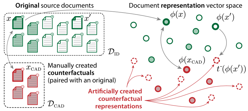
Fig. 1: We propose to generate counterfactuals in representation space, learning — from only a few manually created counterfactuals — a mapping function $t$ to transform a document representation $\phi(x)$ to a counterfactual one (having the opposite classification label). Illustration for positively labeled originals only.

For mitigating the spurious pattern effect, generic methods include regularization of masked language models, which limits over-reliance on a limited set of keywords Moon et al. (2021). Alternatively, to improve robustness in imbalanced data settings, additional training samples can be automatically created Han et al. (2021). Other approaches rely on adding extra training data by human annotation. Specifically to avoid spurious patterns, Kaushik et al. (2019) proposed Counterfactually Augmented Data (CAD), where annotators minimally revise training data to flip their labels: training on both original and counterfactual samples reduced spurious patterns. Rather than editing existing samples, Katakkar et al. (2021) propose to annotate them with text spans supporting the assigned labels as a “rationale” Pruthi et al. (2020); Jain et al. (2020), thus achieving increased performance on OOD data. Similar in spirit, Wang and Culotta (2020) have an expert annotating spurious vs. causal sentiment words and use word-level classification (spurious vs. genuine) to train robust classifiers that only rely on non-spurious words. The cited works thus demonstrate that unwanted reliance on spurious patterns can be mitigated through extra annotation or (counterfactual) data generation. We further explore the latter option, and specifically focus on sentiment classification, as in Kaushik et al. (2019); Katakkar et al. (2021). Exploiting counterfactuals requires first to (i) generate them, and then (ii) maximally benefit from them in training. For ii, Teney et al. (2020) present a loss term to leverage the relation between counterfactual and original samples. In this paper we focus on i, for which Wu et al. (2021) use experts interacting with a finetuned GPT-2 Radford et al. . Alternatively, Wang et al. (2021); Yang et al. (2021) use a pretrained language model and a sentiment lexicon. Yet, having human annotators to create counterfactuals is still costly (e.g., 5 min/sample, Kaushik et al. (2019)). Thus, we pose the research question (RQ): how to exploit a limited amount of counterfactuals to avoid classifiers relying on spurious patterns? We consider classifiers trained on representations obtained from frozen state-of-the-art sentence encoders Reimers and Gurevych (2019); Gao et al. (2021). We require only a few (human produced) counterfactuals, but artificially create additional ones based on them, directly in the encoding space (with a simple transformation of original instance representations), as sketched in Fig. 1. This follows the idea of efficient sentence transformations in De Raedt et al. (2021).

We compare our approach against using (i) moreoriginal samples and (ii) other models generating counterfactuals. We surpass both i–ii for sentiment classification, with in-distribution and counterfactual training data from IMDb Maas et al. (2011); Kaushik et al. (2019) and OOD-test data from Amazon Ni et al. (2019), SemEval Rosenthal et al. (2017) and Yelp Kaushik et al. (2020).

2 Exploiting Few Counterfactuals

	Original Sample ($x$)	Counterfactually Revised Sample ($x_{\textsc{cad}}$)
negative $\to$ positive	one of the worst ever scenes in a sports movie. 3 stars out of 10.	one of the wildest ever scenes in a sports movie. 8 stars out of 10.
positive $\to$ negative	The world of Atlantis, hidden beneath the earth’s core, is fantastic.	The world of Atlantis, hidden beneath the earth’s core is supposed to be fantastic.

Table 1: Two examples from Kaushik et al. (2019) of counterfactual revisions made by humans for IMDb.

We consider binary sentiment classification of input sentences/documents $x\in\mathcal{X}$, with associated labels $y\in\mathcal{Y}=\{0,1\}$. We denote the training set of labeled pairs $(x,y)$ as $\mathbf{\mathcal{D}}_{\textsc{id}}$, of size $n\triangleq\left|\mathbf{\mathcal{D}}_{\textsc{id}}\right|$. We further assume that for a limited subset of $k\ll n$ pairs $(x,y)$ we have corresponding manually constructed counterfactuals $(x_{\textsc{cad}},y_{\textsc{cad}})$, i.e., $x_{\textsc{cad}}$ is a minimally edited version of $x$ that has the opposite label $y_{\textsc{cad}}=1-y$ (see Table 1 for an example). The resulting set of $k$ counterfactuals is denoted as $\mathbf{\mathcal{D}}_{\textsc{cad}}$. We will adopt a vector representation of the input $\phi(x)$, with $\phi:\mathcal{X}\to\mathbb{R}^{d}$. We aim to obtain a classifier $f:\mathbb{R}^{d}\to\mathcal{Y}$ that, without degrading in-distribution performance, performs well on counterfactual samples and is robust under distribution shift.

2.1 Exploiting Manual Counterfactuals

To learn the robust classifier $f$, we first present well-chosen reference approaches that leverage the $n$ in-distribution samples $\mathbf{\mathcal{D}}_{\textsc{id}}$ and the $k$ counterfactuals $\mathbf{\mathcal{D}}_{\textsc{cad}}$. For all of the models below, we adopt logistic regression, but they differ in training data and/or loss function.

The Paired model only uses the pairs for which we have counterfactuals, i.e., the full set $\mathbf{\mathcal{D}}_{\textsc{cad}}$ but only the corresponding $k$ pairs from $\mathbf{\mathcal{D}}_{\textsc{id}}$.

The Weighted model uses the full set of $n$ originals $\mathbf{\mathcal{D}}_{\textsc{id}}$, as well as all counterfactuals $\mathbf{\mathcal{D}}_{\textsc{cad}}$, but compensates for the resulting data imbalance by scaling the loss function on $\mathbf{\mathcal{D}}_{\textsc{id}}$ by a factor $\frac{k}{n}$.

2.2 Generating Counterfactuals

The basic proposition of our method is to artificially create counterfactuals for the $n-k$ original samples from $\mathbf{\mathcal{D}}_{\textsc{id}}$ that have no corresponding pair in $\mathbf{\mathcal{D}}_{\textsc{cad}}$. For this, we learn to map an original input document/sentence representation $\phi(x)$ to a counterfactual one, i.e., a function $t:\mathbb{R}^{d}\to\mathbb{R}^{d}$. We learn two such functions, $t^{\scalebox{0.5}{$-$}}$ to map representations of positive samples $\phi(x)$ (with $y=1$) to negative counterfactual representations $\phi(x_{\textsc{cad}})$ (with $y_{\textsc{cad}}=0$), and vice versa for $t^{\scalebox{0.5}{$+$}}$. We thus apply $t^{\scalebox{0.5}{$-$}}$ (respectively $t^{\scalebox{0.5}{$+$}}$) to the positive (resp. negative) input samples in $\mathbf{\mathcal{D}}_{\textsc{id}}$ for which we have no manually created counterfactuals.

Mean Offset

Our first model is parameterless, where we simply add the average offset between representations of original positives $x$ (with $y=1$) and their corresponding $x_{\textsc{cad}}$ to those positives for which we have no counterfactuals (and correspondingly for negatives). Thus, mathematically:

$$t^{\scalebox{0.5}{$-$}}(\phi(x))=\phi(x)+\vec{o}_{\scalebox{0.5}{$-$}}\,\mathrm{,with}$$

$$\vec{o}_{\scalebox{0.5}{$-$}}=\operatorname*{avg}_{x\,:\,y=1}\phi(x_{\textsc{cad}})-\phi(x)$$

(and correspondingly for $t^{\scalebox{0.5}{$+$}}$ based on counterfactuals of $x$ for which $y=0$).

Mean Offset + Regression

Since just taking the average offset may be too crude, especially as $k$ increases, we can apply an offset adjustment (noted as $r:\mathbb{R}^{d}\to\mathbb{R}^{d}$) learnt with linear regression. Concretely, to create counterfactuals for positive originals we define:

$$t^{\scalebox{0.5}{$-$}}(\phi(x))=\phi(x)+\vec{o}_{\scalebox{0.5}{$-$}}+r^{\scalebox{0.5}{$-$}}(\phi(x))$$

with a linear function

$$r^{\scalebox{0.5}{$-$}}(\phi(x))=W^{\scalebox{0.5}{$-$}}\cdot\phi(x)+b^{\scalebox{0.5}{$-$}}$$

(learning $W^{\scalebox{0.5}{$-$}}\in\mathbb{R}^{d\times d}$ and $b^{\scalebox{0.5}{$-$}}\in\mathbb{R}^{d}$ from the positive originals $x$ with corresponding counterfactuals $x_{\textsc{cad}}$) and $\vec{o}_{\scalebox{0.5}{$-$}}$ as defined above. Similarly for $t^{\scalebox{0.5}{$+$}}$.

3 Experimental Setup

	SimCSE-RoBERTalarge				SRoBERTalarge
Model    ($n$) ($k$)	Orig. (%)	CAD (%)	OOD (%)	Avg.	Orig. (%)	CAD (%)	OOD (%)	Avg.
Original  (3.4k) (0)	89.6±0.7	75.7±1.2	74.6±2.6	80.0	90.7±0.6	78.8±1.7	80.6±2.4	83.4
Weighted  (1.7k) (16)	88.1±0.8	78.5±1.1	75.1±2.3	80.6	89.2±0.8	81.1±1.3	82.9±2.1	84.4
Paired  (16) (16)	81.5±2.2	80.9±2.4	77.5±4.3	80.0	86.9±1.3	77.9±2.2	83.9±4.2	82.9
Wang and Culotta (2021):  (1.7k) (0)
- Pred. from top  ($n^{\prime\prime}$=1,284)	81.4	82.6	73.0	79.0	83.6	83.4	73.4	80.1
- Ann. from top  ($n^{\prime\prime}$=1,618)	80.3	84.2	74.1	79.5	81.8	86.1	71.2	79.7
- Ann. from all  ($n^{\prime\prime}$=1,694)	83.0	85.7	76.5	81.7	85.7	89.8	75.6	83.7
Our models:  (1.7k) (16)
- Mean Offset	86.2±1.2	84.6±1.3	78.0±3.2	83.0	88.1±1.2	85.6±1.1	83.0±3.3	85.6
- Mean Offset + Regression	86.1±1.2	84.1±1.3	78.2±3.1	82.8	88.3±1.0	85.2±1.5	83.4±3.3	85.6

Table 2: Results with $k$ = 16 manually crafted counterfactuals and $n$ original samples. Note that our models then use an additional $n^{\prime}=n-k$ artificial counterfactuals generated in representation space. The models of Wang and Culotta (2021) automatically generate $n^{\prime\prime}$ counterfactuals in the input space.

Datasets

For the in-distribution data, we use a training set $D_{\textsc{id}}^{\textit{train}}$ of 1,707 samples, and a test set $D_{\textsc{id}}^{\textit{test}}$ of 488 samples, with all of these instances randomly sampled from the original IMDb sentiment dataset of 25k reviews Maas et al. (2011). The counterfactual sets $D_{\textsc{cad}}^{\textit{train}}$ and $D_{\textsc{cad}}^{\textit{test}}$ are the revised versions of $D_{\textsc{id}}^{\textit{train}}$ and $D_{\textsc{id}}^{\textit{test}}$, as rewritten by Mechanical Turk workers recruited by Kaushik et al. (2019). See Appendix B for further details. We will also test on out-of-distribution (OOD) data from Amazon Ni et al. (2019), SemEval Rosenthal et al. (2017) and Yelp Kaushik et al. (2020) (we note these datasets as $D_{\textsc{ood}}^{\textsc{amzn}}$, $D_{\textsc{ood}}^{\textsc{se}}$, $D_{\textsc{ood}}^{\textsc{yelp}}$).

Sentence Encoders

To obtain $\phi(x)$, we use the sentence encoding frameworks SBERT and SimCSE (Reimers and Gurevych (2019); Gao et al. (2021)). The main results are presented with SRoBERTa_large and SimCSE-RoBERTa_large and they are kept frozen at all times. Appendix B lists additional details; Appendix A shows results for other encoders.

Baselines

As a baseline for our few-counterfactuals-based approaches, we present results (Original) from a classifier trained on twice the amount of original (unrevised, in-distribution) samples. Further, we also investigate competitive counterfactual-based approaches as proposed by Wang and Culotta (2021), who leverage identified causal sentiment words and a sentiment lexicon to generate counterfactuals in the input space (which we subsequently embed with the same sentence encoders $\phi$ as before). They adopt three settings, with increasing human supervision, to identify causal words: (i) predicted from top: 32 causal words were identified automatically for IMDb; (ii) annotated from top: a human manually marked 65 words as causal from a top-231 word list deemed most relevant for sentiment; and (iii) annotated from all: a human labeled 282 causal words from the full 2,388 word vocabulary.

Training and Evaluation

For all presented approaches, the classifier $f$ is implemented by logistic regression with L2 regularization, where the regularization parameter $\lambda$ is established by 4-fold cross-validation. The results presented further in the main paper body report are obtained by training on the complete training set (i.e., all folds).

The Mean Offset + Regression model of §2.2, to artificially generate counterfactuals, is implemented by linear regression with ordinary least squares. The Weighted and Paired classifiers of §2.1 are trained on $n$ samples from $D_{\textsc{id}}^{\textit{train}}$ together with $k$ counterfactuals sampled from $D_{\textsc{cad}}^{\textit{train}}$. To evaluate our classifiers with generated counterfactuals, as described in §2.2, we train on the $n$ original samples, $k$ manual counterfactuals and $n-k$ generated counterfactuals. The Original baseline uses $2\cdot n$ original samples $D_{\textsc{id}}^{\textit{train}}\cup D_{\textsc{id}}^{\textit{train}}\,{}^{\prime}$, adding an extra $|D_{\textsc{id}}^{\textit{train}}\,{}^{\prime}|=n$ that are sampled randomly from the 25k original, unrevised IMDb reviews (but not in $D_{\textsc{id}}^{\textit{train}}$ and $D_{\textsc{id}}^{\textit{test}}$). For the counterfactual-based models of Wang and Culotta (2021), the training set is expanded with $n^{\prime\prime}\approx n$ counterfactuals (based on $D_{\textsc{id}}^{\textit{train}}$) automatically generated, in the input space.

We evaluate the accuracy on $D_{\textsc{id}}^{\textit{test}}$, $D_{\textsc{cad}}^{\textit{test}}$ and the OOD test sets $D_{\textsc{ood}}^{\textsc{amzn}}$, $D_{\textsc{ood}}^{\textsc{se}}$, $D_{\textsc{ood}}^{\textsc{yelp}}$ (averaging the accuracies over these 3 sets for OOD evaluation). For each $k\in\{16,32,\ldots,128\}$, we use 50 different random seeds to sample: (i) $k/2$negative and $k/2$ positive counterfactuals, and (ii) $n$additional original samples (for Original baseline). The reported accuracies are averaged across the 50 seeds.

4 Results and Discussion

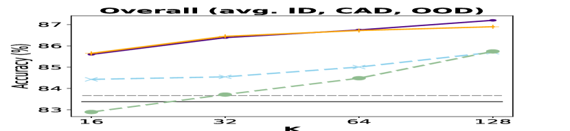
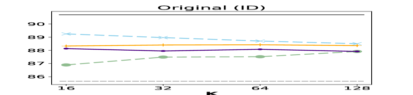
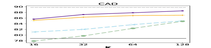
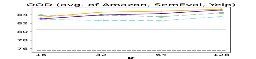
Fig. 2: Accuracies for an increasing number of manually crafted counterfactuals $k$ for SRoBERTa_large-based models. From Wang and Culotta (2021), we selected the best performing model (Annotated from all).

Main Results

We investigate if a limited amount of counterfactuals suffices to make classifiers less sensitive to spurious patterns: classification should also perform well on counterfactual and OOD examples, without sacrificing in-distribution (ID) performance.

Figure 2 and Table 2 report on the accuracies for the different models on the original ($D_{\textsc{id}}^{\textit{test}}$), counterfactual ($D_{\textsc{cad}}^{\textit{test}}$) and OOD test sets (avg. over $D_{\textsc{ood}}^{\textsc{amzn}}$, $D_{\textsc{ood}}^{\textsc{se}}$, $D_{\textsc{ood}}^{\textsc{yelp}}$). The average of these three values is plotted as the overall metric in the leftmost panel of Fig. 2 and the Avg. column in Table 2. From this overall perspective, we note that our classifiers trained on offset-based counterfactuals outperform the Original baseline trained on 3.4k samples by +3% (+2.2%) points in accuracy for SimCSE-RoBERTa_large (SRoBERTa_large), even when the number of manually crafted counterfactuals is less than 1% (i.e., for $k$ = 16) of the original sample size ($n$ = 1.7k). Moreover, we note that all counterfactual-based classifiers improve for increasing numbers of counterfactuals $k$. We observe little difference between the performance of classifiers trained on generated counterfactuals from the Mean Offset and the Mean Offset + Regression models, with the former working slightly better than the latter for larger $k$, indicating that the simple mean offset is a good choice. Moreover, our classifiers trained on offset-based counterfactuals of SimCSE-RoBERTa_large (SRoBERTa_large) show a clear improvement over both classifiers (i) without generated counterfactuals (+2.4% (+1.2%) over Weighted and +3% (+2.7%) over Paired), and (ii) trained on counterfactuals generated with the best model of Wang and Culotta (2021) (improving by +1.3% (+1.9%)). (ii) relies on annotating a 2,388 word vocabulary (which we speculate to be more labor-intensive than creating just 16 counterfactuals; poor Predicted (Annotated) from top results suggest we cannot avoid human annotation).

We further compare the models to the Original baseline on the three test subsets (ID, CAD, OOD). For straightforward imbalance counteracting strategies (Paired, Weighted), we observe expected performance improvement of SimCSE-RoBERTa_large (SRoBERTa_large) for data that deviates from the ID training data, i.e., for OOD and CAD — yet, clearly more advanced methods like ours do way better — while sacrificing performance for ID itself. We find that the best Wang and Culotta (2021) model excels at CAD with improvements of +10% (+11%), but by doing so suffers a lot on ID $-$6.6% ($-$5%) and on OOD +1.9% ($-$5%). In contrast, our Mean Offset model strikes the desirable balance across ID, CAD, and OOD performance with a smaller drop in ID accuracy of $-$3.4% ($-$2.6%), and with improvements on both CAD and OOD of respectively +8.9% (+6.8%) and +3.4% (+2.4%).

Ablations

	SimCSE-RoBERTalarge				SRoBERTalarge
Model    ($n$) ($k$)	Orig. (%)	CAD (%)	OOD (%)	Avg.	Orig. (%)	CAD (%)	OOD (%)	Avg.
Ablation models:
- Random Offset (1.7k) (0)	87.7±0.7	74.3±1.0	73.1±2.6	78.3	88.6±1.0	77.9±1.3	79.0±3.3	81.8
- Meanid Offset (1.7k) (0)	88.9±0.3	76.1±0.2	73.8±0.2	79.6	88.4±0.3	79.0±0.2	78.9±0.8	82.1
- Linear Regression (1.7k) (16)	88.2±0.9	77.8±1.5	74.9±2.4	80.3	89.5±0.8	81.8±1.0	83.2±1.7	84.8
Our models:  (1.7k) (16)
- Mean Offset	86.2±1.2	84.6±1.3	78.0±3.2	83.0	88.1±1.2	85.6±1.1	83.0±3.3	85.6
- Mean Offset + Regression	86.1±1.2	84.1±1.3	78.2±3.1	82.8	88.3±1.0	85.2±1.5	83.4±3.3	85.6

Table 3: Ablations ($k$ = 16): A comparison of our models with models that generate counterfactuals by (i) adding a random offset (with same L2-norm as the mean offset) to original samples, (ii) adding the mean offset calculated between the $n$ original samples with opposite labels (without $k$ counterfactuals) to original samples or (iii) by transforming the original samples directly with linear regression (i.e., without the mean offset).

To investigate the effectiveness of our Mean Offset (+ Regression) approaches that exploit $k$ manually crafted counterfactuals, we provide ablations by including the scores for counterfactuals generated with (i) a Random Offset with the same L2-norm as the mean offset, (ii) a Mean_id Offset calculated among the $n$ original samples with opposite labels (and thus without $k$ manual counterfactuals), and (iii) a mapping function $t$ modeled directly with Linear Regression, i.e., $t(\phi(x))=W\cdot\phi(x)+b$ (with $b\in\mathbb{R}$, $W\in\mathbb{R}^{d\times d}$).

Following §3, we randomly sample 50 times: random offsets, and $k$ (original, counterfactual) pairs from $D_{\textsc{id}}^{\textit{train}}$ and $D_{\textsc{cad}}^{\textit{train}}$ from which the Mean Offset is calculated and from which the parameters of Mean Offset + Regression are learnt.

The classification accuracies for the ablation models are shown in Table 3, demonstrating the importance of using counterfactuals to calculate an effective offset: the Mean Offset consistently outperforms the Random Offset and the Mean_id Offset (both calculated without manual counterfactuals). Since the Random Offset shifts in a totally arbitrary direction, it does not produce very useful “counterfactuals” to learn from. As the Mean_id Offset is calculated among the $n$ original samples, it does not provide “new” information that was not already present in the original samples.

At last, we observe expected performance improvement for the Mean Offset (+ Regression) over the Linear Regression model since directly learning its transformation matrix ($W\in\mathbb{R}^{d\times d}$) from just $k$ (=16) (original, counterfactual) pairs is difficult.

5 Conclusion

We explored improving the robustness of classifiers (i.e., make them perform well also on out-of-distribution, OOD, data) by relying on just a few manually constructed counterfactuals. We propose a simple strategy, learning from few (original, counterfactual) pairs how to transform originals $\mathbf{\mathcal{D}}_{\textsc{id}}$ into counterfactuals $\mathbf{\mathcal{D}}_{\textsc{cad}}$, in a document vector representation space: shift an original document with the mean offset among the given pairs. Thus, using just a small number (1% of $|\mathbf{\mathcal{D}}_{\textsc{id}}|$) of manual counterfactuals, we outperform sentiment classifiers trained using either (i) 100% extra original samples, or (ii) a state-of-the-art (lexicon-based) counterfactual generation approach. Thus, we suggest that additional annotation budget is better spent on counterfactually revising available annotations, rather than collecting similarly distributed new samples.

Limitations

Our work is limited in terms of interpretability, the trade-off between computational efficiency and model effectiveness, and the application domain of the presented experiments. These limitations are discussed in the following paragraphs.

Interpretability

Our models produce counterfactual samples directly in the encoding vector space, and they thus cannot easily be interpreted. One could train a decoder to reconstruct the IMDb documents from the frozen vector representations. However, we believe it to be infeasible given (i) the considerable length of the IMDB documents (more than 160 words on average), and (ii) the fact that the document would need to be decoded from a single vector without relying, e.g., on the attention mechanism (since the decoder should otherwise bypass the single vector representation) . Thus, it would be hard to discern whether observed noise in the reconstructed full review documents is due to flaws in our generated vectors, or rather the imperfect decoder. Hence, we opted for the quantitative analysis in Appendix A.2 instead.

Efficiency vs. effectivenes

Our methods generate counterfactual vectors in the encoding space of frozen sentence encoders such that the attained accuracy, while competitive, may be lower than when compared to fully fine-tuned transformers. However, leveraging frozen sentence encoders allows us to train way faster (<1 minute on CPU): the linear sentiment classification layer contains less than 2K parameters, estimating the mean offset is parameterless, and the linear transformation of the mean offset + regression model contains less than 1.2M parameters. In contrast, fully finetuning BERT requires updating all 110M parameters for 20 epochs on a Tesla V100 GPU Kaushik et al. (2019). In addition, using pre-trained frozen sentence encoders allows us to analyze whether their produced embeddings are able to model the subtle differences between original and counterfactual samples, and whether this difference can be exploited to improve robustness.

Application domain

We presented results for sentiment classification, given that, to the best of our knowledge, the only topic classification datasets with paired counterfactual training samples is IMDb Kaushik et al. (2019). However, we believe that our method could generalize beyond sentiment classification to other topic classification tasks for which there is a clear direction in the vector space between different topics (=classes), such as from positive to negative (or vice versa). Note that this is not the case for the Natural Language Inference (NLI) task. Hence, why we did not experiment on existing NLI datasets with available counterfactuals Kaushik et al. (2019).

Appendices

Appendix A Additional Results

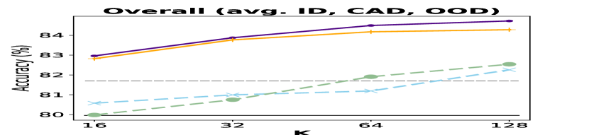
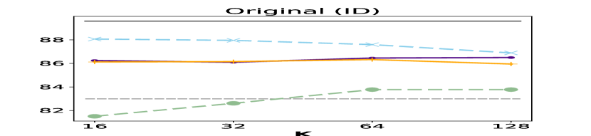
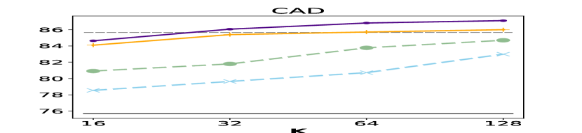
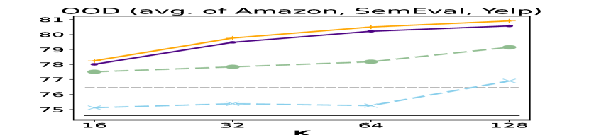
Fig. 3: SimCSE-RoBERTa_large

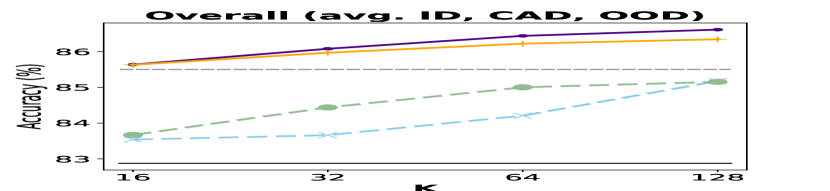
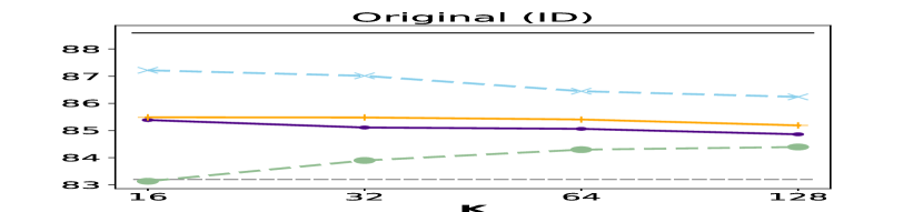
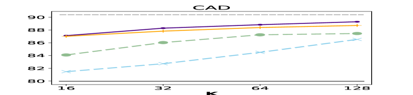
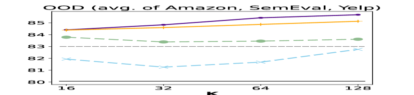
Fig. 4: SimCSE-BERT_large

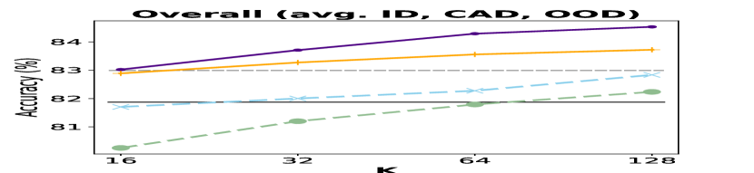
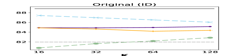
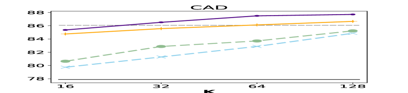
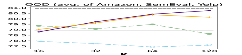
Fig. 5: SimCSE-BERT_base

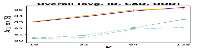
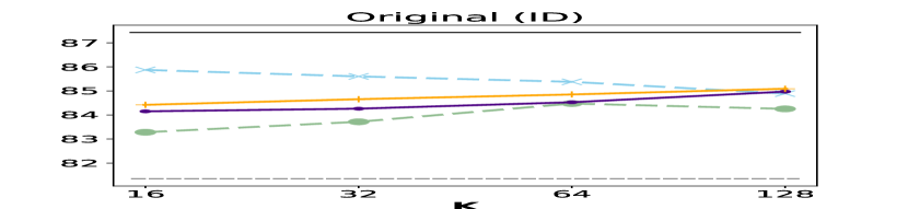
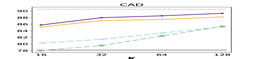
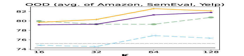
Fig. 6: SDistillRoBERTa

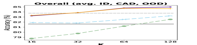
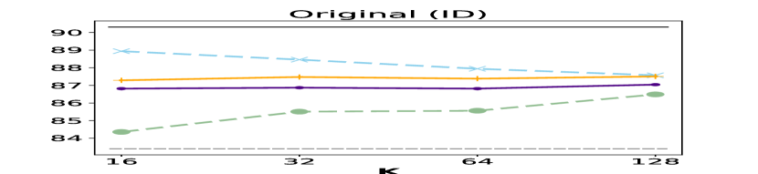
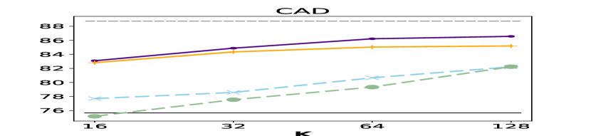
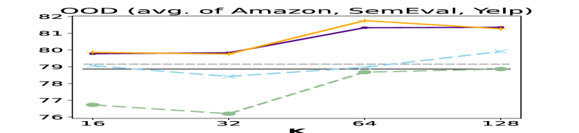
Fig. 7: SMPNet

We provide additional results for other sentence encoders (i) for an increasing number of counterfactuals $k$ in Figs. 3–7 and (ii) for $k=16$ in Tables 7–12. We discuss the impact of regularization in §A.1, provide an analysis of the generated counterfactuals in §A.2, discuss the overall robustness in §A.3, and compare the strengths and weaknesses of the different approaches in §A.4.

A.1 Impact of Regularization Strength

The methods using generated counterfactuals expand the original training set $D_{\textsc{id}}^{\textit{train}}$ with counterfactuals $D_{\textsc{cad}}^{\textit{train}}$. Our models add $k$ manually crafted ones and $n-k$ generated ones, whereas the state-of-the-art models Wang and Culotta (2021) add $n^{\prime\prime}\approx n$ generated ones. When using both ID and CAD samples for training, we risk overfitting to the generated counterfactuals (which may be more narrowly distributed than data in the wild, for which the OOD and CAD test samples are a proxy). Such overfitting can be avoided by enforcing stronger L2 regularization (i.e., larger $\lambda$). We analyze whether this is useful and experiment by either (i) free regularization, allowing a broad range spanning both weak and strong regularization $\lambda\in\{10^{-3},10^{-2},\ldots,10^{3}\}$, or (ii) strong regularizationrestricting the choice to $\lambda\in\{1,10,\ldots,10^{3}\}$. Tables 7–12 show the results for such free vs. strong regularization. We note that both model types using artificially generated counterfactuals (ours and Wang and Culotta (2021)) generally benefit from strong regularization, whereas the others perform better under free regularization (suggesting they are less prone to overfitting). We note that especially models based on Wang and Culotta (2021) may suffer from overfitting (e.g., a difference of almost 14 percentage points on OOD accuracy even for their best model, Ann. from all, based on SimCSE-RoBERTa_large). In conclusion, as main paper results we therefore reported the results of the best free regularization $\lambda$ choice for models without generated counterfactuals, whereas for ours and Wang and Culotta (2021) we reported strong regularization results.

A.2 Analysis of Generated Counterfactual Vectors

	SimCSE-RoBERTalarge			SRoBERTalarge
Samples	R2	RMSE	Diversity	R2	RMSE	Diversity
Original samples ($D_{\textsc{id}}^{\textit{test}}$)	$-$0.747$\,\downarrow$	$0.000\,132\,2$	0.549$\,\downarrow$	0.797	$0.000\,121\,4$	0.627$\,\downarrow$
Manual Counterfactuals ($D_{\textsc{cad}}^{\textit{test}}$)	-	-	0.539$\,\downarrow$	-	-	0.621$\,\downarrow$
Generated from ablation models:
- Linear Regression	$-$0.066 $\downarrow$	$0.023\,227\,8$	0.087 $\downarrow$	$-$0.068$\,\downarrow$	$0.025\,178\,8$	0.092$\,\downarrow$
- Random Offset	$-$0.654$\,\downarrow$	$0.012\,632\,5$	0.524 $\downarrow$	$-$0.724 $\downarrow$	$0.012\,193\,9$	0.601$\,\downarrow$
Generated from our models:
- Mean Offset	$+$0.785 $\uparrow$	$0.010\,325\,5$	0.537$\,\approx$	$-$0.830 $\uparrow$	$0.009\,916\,1$	0.619$\,\approx$
- Mean Offset + Regression	$+$0.779$\,\uparrow$	$0.010\,473\,7$	0.536$\,\approx$	$+$0.821$\,\uparrow$	$0.010\,180\,2$	0.618$\,\approx$

Table 4: Analysis of generated counterfactuals ($k$ = 16): R² and RMSE scores between the encoded samples of $D_{\textsc{ID}}^{\textit{test}}$ and $D_{\textsc{cad}}^{\textit{test}}$ as a reference (in bold), and between the generated counterfactuals and encodings in $D_{\textsc{cad}}^{\textit{test}}$, where $\uparrow$ and $\downarrow$ denote values higher or lower than the reference. We compare diversity of the generated counterfactuals compared to that of the encodings of manually crafted ones ($D_{\textsc{cad}}^{\textit{test}}$) (in bold), where $\approx$ and $\downarrow$ respectively denote similar and lower diversity.

Since our methods produce counterfactuals in the encoding space, they cannot be easily interpreted. Still, we attempt to analyze how well they are aligned with manual constructed counterfactuals. To do so we measure (i) the coefficient of determination, R², and (ii) the root mean squared error (RMSE) between the generated and manual counterfactual test vectors. Both metrics quantify how well the generated vectors approximate manual counterfactual vectors. In addition, we provide a measure of diversity, calculated as the average pairwise cosine distance among generated samples: we compare it against that diversity among vectors of the manually constructed counterfactuals. A well approximated set of generated counterfactuals should be as diverse as a manually constructed set, and approach the unrevised originals’ diversity.

Setup

Following the same setup as in §3, we randomly sample 50 times: $k$ (original, counterfactual) pairs from $D_{\textsc{id}}^{\textit{train}}$ and $D_{\textsc{cad}}^{\textit{train}}$, from which the Mean Offset is calculated and from which the parameters of the Mean Offset + Regression are learned. We apply both transformations on the original test encodings ($D_{\textsc{id}}^{\textit{test}}$) to generate counterfactuals and compare them to the encodings of the manual test samples ($D_{\textsc{cad}}^{\textit{test}}$).

Moreover, we provide an ablation by including the scores for counterfactuals generated with two ablation models of §4, i.e., (i) a Random Offset (with same L2-norm as the mean offset), (ii) a mapping function $t$ modeled directly Linear Regression, i.e., $t(\phi(x))=W\cdot\phi(x)+b$ (with $b\in\mathbb{R}$, $W\in\mathbb{R}^{d\times d}$).

We also report the R² and RMSE scores between the original encodings and their manually revised counterparts, which we use as a reference to determine to what extent generated counterfactual encodings align with those of manually crafted counterfactuals.

Results

The results are shown in Table 4 (averaged over the 50 runs). First, we assess how well the generated counterfactuals approximate the manual ones using R² scores. We observe that R² between the original samples and their corresponding manual counterfactual already reaches 0.747 and 0.797 for SimCSE-RoBERTa_large and SRoBERTa_large respectively. This is not surprising, since only a minimal number of words are edited in revising an original sample to its counterfactual. The generated counterfactuals improve over the original score, with R² scores for the Mean Offset (+ Regression) of 0.785 (0.779) and 0.830 (0.821), respectively for SimCSE-RoBERTa_large and SRoBERTa_large. Conversely, the ablation models result in counterfactuals more dissimilar than the originals (even lower R² than our models), with especially the Linear Regression model performing poorly. Additionally, the RMSE-scores for our models are notably lower than those from the ablation models, but clearly larger than the (very low, because of minimal edits) RMSE for manual counterfactuals.

Second, we assess that the generated counterfactuals preserve the original diversity for both encoders, with scores for the Mean Offset (+ Regression) method of 0.537 (0.536) and 0.619 (0.618) that are very close to those for the manual counterfactuals (0.539 and 0.621, respectively for the two encoders). The ablation models on the other hand attain lower diversity scores, with especially Linear regression behaving extremely poorly — which we suspect to be caused by a collapse where the same subset of vectors are predicted regardless the input.

Third, when looking at both Table 3 (classification accuracies for the ablation models §4) and Table 4, we observe that the Linear Regression model outperforms Random Offset overall in terms of attained accuracies (given its better performance for CAD and OOD), even though Random Offset’s “better” counterfactuals (cf. higher R² and lower RMSE in Table 4) may lead one to expect the opposite. We speculate that, given the very low diversity, the Linear Regression model just predicts the set of $k$ counterfactuals which it saw during training, making it more similar to the Weighted model that does not train with generated counterfactuals.

A.3 Overall Robustness

	SimCSE-RoBERTalarge				SRoBERTalarge
Model    ($n$) ($k$)	Orig. (%)	CAD (%)	OOD (%)	Avg.	Orig. (%)	CAD (%)	OOD (%)	Avg.
- Original (3.4k) (0)	89.6±0.7	75.7±1.2	74.6±2.6	80.0	90.7±0.6	78.8±1.7	80.6±2.4	83.4
- Original (24k) (0)	91.1±0.0	78.5±0.0	77.8±0.0	82.5	92.6±0.0	80.1±0.0	80.9±0.0	84.6
Our Models:  (1.7k) (16)
- Mean Offset	86.2±1.2	84.6±1.3	78.0±3.2	83.0	88.1±1.2	85.6±1.1	83.0±3.3	85.6
- Mean Offset + Regression	86.1±1.2	84.1±1.3	78.2±3.1	82.8	88.3±1.0	85.2±1.5	83.4±3.3	85.6

Table 5: Baseline trained with all original samples: A comparison of our offset-based models to the Original classifier trained on all 24k original samples.

From the leftmost graphs in Figs. 3–7, we observe that the different classifiers follow the main trends as discussed in §4: the models trained on generated counterfactual vectors from the mean offset models, are overall most robust and outperform both (i) classifiers without generated counterfactuals (Weighted and Paired) and (ii) classifiers trained on counterfactuals generated from the best model of Wang and Culotta (2021). This holds for all sentence encoders and values of $k\in\{$16, 32, 64, 128$\}$, with the sole exception of SMPNet and SimCSE-BERT${}_{\texttt{base}}$ for which Annotated from all (based on Wang and Culotta (2021)) is slightly better than the offset-based models for $k=$ 16, but still worse when $k>$ 16. Hence, we stand by the main paper’s stated conclusions.

Furthermore, Table 5 highlights that classifiers trained on our offset-based counterfactuals (using 1.7k original and just $k=$ 16 manual counterfactuals) can outperform the Original baseline trained on all 24k original samples (most clear for SRoBERTa_large). It is worth noting that the Original baseline becomes more robust when trained on all 24k original samples rather than 3.4k samples. However, to make the Original classifier more robust requires annotating 22.3k extra in-distribution samples, rather than counterfactually revising only 16 original samples.

A.4 Strengths and Weaknesses

Below we discuss the strengths and weaknesses of the different approaches by considering all sentence encoders.

Paired

Following the results in §4, the Paired approach consistently yields high accuracies on the out-of-distribution (OOD) test set: for all encoders we observe a notable improvement over the Original classifier, with SMPNet as the exception. Moreover, the Paired model reaches similar or even slightly better OOD performance compared to the best approaches for small values $k\in\{$16, 32$\}$. However, when evaluated on in-distribution (ID) samples, the Paired model degrades significantly in accuracy compared to the Original classifier and the majority of all other approaches. For counterfactuals (CAD), the Paired model improves upon the Original classifier but performs worse than the approaches that train with generated counterfactuals (i.e., ours and Wang and Culotta (2021)).

Weighted

We observe similar trends as discussed in §4 where the Weighted model retains most of the Original classifier’s performance on in-distribution samples, and more so than any of the other approaches. While Weighted performs better than the Original model on CAD it performs significantly worse than the classifiers trained with generated counterfactuals. The generalization of Weighted to out-of-distribution is mixed, where only for some encoders it yields slightly better results than the Original classifier, but it is consistently worse when compared to the Paired model and classifiers trained with generated counterfactuals from our models.

Annotated from top

Wang and Culotta (2021) The results for other sentence encoders, again, are similar to those reported in §4. The classifier trained with counterfactuals from this model degrades significantly on in-distribution performance, more than any of the other approaches except for SimCSE-BERT_base and SimCSE-BERT_large, where the Paired model performs worse for $k<$ 64. For CAD, this model is the most accurate compared to the other approaches (with $k=$ 16). Except for SimCSE-BERT_base, the classifiers tends to generalize worse for OOD-samples compared to our approaches that train on generated counterfactuals, and for SRoBERTa_large worse than the Original classifier.

Mean Offset (+Regression)

The classifiers trained with counterfactuals generated from our models slightly drop in accuracy on in-distribution samples but perform better, except the Weighted model, than all the other approaches. On CAD, the classifiers perform either best or come in second to the best model from Wang and Culotta (2021). Similarly, they perform best or come in second to the Paired model for OOD (except for SimCSE-BERT_base for which Wang and Culotta (2021) is better). Note that our offset-based models, with a slight drop in in-distribution accuracy but consistent improvements on both CAD and OOD data, results in classifiers that strike the desirable balance across the three different test distributions (ID, CAD, OOD).

Appendix B Experimental Details

Dataset	# Documents	# Tokens (avg.)
In-distribution
- IMDb train ($D_{\textsc{ID}}^{\textit{train}}$)	1,707	163
- IMDb test ($D_{\textsc{ID}}^{\textit{test}}$)	488	162
Counterfactual
- IMDb train ($D_{\textsc{CAD}}^{\textit{train}}$)	1,707	162
- IMDb test ($D_{\textsc{CAD}}^{\textit{test}}$)	488	162
Out-of-distribution
- Amazon test ($D_{\textsc{ood}}^{\textsc{amzn}}$)	5,766	132
- Yelp test ($D_{\textsc{ood}}^{\textsc{yelp}}$)	6,462	120
- SemEval test ($D_{\textsc{ood}}^{\textsc{se}}$)	130,126	20

Table 6: Dataset statistics

Datasets

Table 6 summarizes the dataset statitics, reporting per dataset/split: (i) the number of documents and (ii) the average number of tokens per document. All datasets are equally balanced between the positive and negative classes.

Sentence Encoders

For the SBERT architecture, we reported results for models based on RoBERTa Liu et al. (2019), DistilRoBERTa, and MPNet Song et al. (2020) with corresponding Hugging Face Wolf et al. (2020) identifiers: all-roberta-large-v1, all-distilroberta-v1 and all-mpnet-base-v2. For SimCSE, we experimented with models based on RoBERTa_large Liu et al. (2019), BERT_large and based on BERT_large Devlin et al. (2019), with as Hugging Face names unsup-simcse-roberta-large, unsup-simcse-bert-large and unsup-simcse-bert-base. Before training the linear classifiers on CPU, we pre-computed all the encodings for the different datasets on a single GeForce GTX 1080 Ti, taking at most one hour for each encoder. All sentence encoders yield vectors of dimension $d$ ranging between 768 and 1,024.

Linear Classifiers

As stated before, classifiers in the experiments are trained with logistic regression and 4-fold cross-validation (to determine L2 regularization parameter $\lambda$) for which we used the LogisticRegressionCV implementation of Scikit-Learn Pedregosa et al. (2011). We choose the ‘lbfgs’ solver, set the maximum number of iterations to 4,000, and used for the ‘Cs’ parameter the inverse regularization values of those reported in the paper. The classifiers can easily be trained and evaluated on all datasets on a 2,6 GHz 6-Core Intel Core i7, taking less than one minute per run.

Linear Regression

We implemented the Mean Offset + Regression model using the LinearRegression implementation of Sklearn with default parameters and ordinary least squares. Computing both the mean offset and the transformation gives negligible overhead and can be done within a fraction of a second on a on a 2,6 GHz 6-Core Intel Core i7 CPU.

Code

Our code and data to reproduce the experimental results is publicly available.

SRoBERTalarge
	Free Reg.: $\lambda\in\{10^{-3},10^{-2},\ldots,10^{3}\}$				Strong Reg.: $\lambda\in\{1,10,\ldots,10^{3}\}$
Model    ($n$) ($k$)	Orig. (%)	CAD (%)	OOD (%)	Avg.	Orig. (%)	CAD (%)	OOD (%)	Avg.
Original (3.4k)(0)	90.7±0.6	78.8±1.7	80.6±2.4	83.4	90.1±0.5	76.8±1.0	79.1±2.1	82.0
Weighted  (1.7k) (16)	89.2±0.8	81.1±1.3	82.9±2.1	84.4	81.7±3.0	72.0±4.7	76.3±6.6	76.7
Paired  (16) (16)	86.9±1.3	77.9±2.2	83.9±4.2	82.9	87.0±1.4	77.4±2.2	84.4±3.5	82.9
Wang and Culotta (2021):  (1.7k) (0)
- Pred. from top  ($n^{\prime\prime}$=1,284)	80.5	78.1	66.6	75.1	83.6	83.4	73.4	80.1
- Ann. from top  ($n^{\prime\prime}$=1,618)	77.9	82.4	65.6	75.3	81.8	86.1	71.2	79.7
- Ann. from all  ($n^{\prime\prime}$=1,694)	80.5	81.6	68.5	76.9	85.7	89.8	75.6	83.7
Our models:  (1.7k) (16)
- Mean Offset	87.7±1.3	84.5±2.0	80.5±4.4	84.2	88.1±1.2	85.6±1.1	83.0±3.3	85.6
- Mean Offset + Regression	88.5±1.0	84.7±1.8	82.0±4.0	85.1	88.3±1.0	85.2±1.5	83.4±3.3	85.6

Table 7: SRoBERTa_large

SimCSE-RoBERTalarge
	Free Reg.: $\lambda\in\{10^{-3},10^{-2},\ldots,10^{3}\}$				Strong Reg.: $\lambda\in\{1,10,\ldots,10^{3}\}$
Model    ($n$) ($k$)	Orig. (%)	CAD (%)	OOD (%)	Avg.	Orig. (%)	CAD (%)	OOD (%)	Avg.
Original (3.4k)(0)	89.6±0.7	75.7±1.2	74.6±2.6	80.0	88.2±0.6	73.9±0.9	73.9±2.0	78.7
Weighted  (1.7k) (16)	88.1±0.8	78.5±1.1	75.1±2.3	80.6	77.5±3.0	75.5±3.5	72.8±4.6	75.3
Paired  (16) (16)	81.5±2.2	80.9±2.4	77.5±4.3	80.0	81.2±1.9	79.8±3.0	78.0±4.2	79.7
Wang and Culotta (2021):  (1.7k) (0)
- Pred. from top  ($n^{\prime\prime}$=1,284)	79.3	73.2	61.2	71.2	81.4	82.6	73.0	79.0
- Ann. from top  ($n^{\prime\prime}$=1,618)	78.5	76.4	59.4	71.5	80.3	84.2	74.1	79.5
- Ann. from all  ($n^{\prime\prime}$=1,694)	80.1	81.1	62.6	74.6	83.0	85.7	76.5	81.7
Our models:  (1.7k) (16)
- Mean Offset	87.0±1.0	81.6±1.4	74.1±2.7	80.9	86.2±1.2	84.6±1.3	78.0±3.2	83.0
- Mean Offset + Regression	87.1±1.4	82.5±1.8	75.6±3.1	81.7	86.1±1.2	84.1±1.3	78.2±3.1	82.8

Table 8: SimCSE-RoBERTa_large

SDistilRoBERTa
	Free Reg.: $\lambda\in\{10^{-3},10^{-2},\ldots,10^{3}\}$				Strong Reg.: $\lambda\in\{1,10,\ldots,10^{3}\}$
Model    ($n$) ($k$)	Orig. (%)	CAD (%)	OOD (%)	Avg.	Orig. (%)	CAD (%)	OOD (%)	Avg.
Original (3.4k)(0)	87.4±0.8	78.2±1.8	74.3±3.7	80.0	87.2±0.6	74.8±0.8	72.7±2.7	78.2
Weighted  (1.7k) (16)	85.9±0.8	80.3±1.2	74.8±3.2	80.3	77.1±3.2	72.6±3.2	72.6±8.0	74.1
Paired  (16) (16)	83.3±2.0	78.0±2.8	80.0±5.6	80.4	83.7±2.1	77.0±2.9	80.7±5.5	80.5
Wang and Culotta (2021):  (1.7k) (0)
- Pred. from top  ($n^{\prime\prime}$=1,284)	73.6	84.4	65.8	74.6	78.3	85.7	74.9	79.6
- Ann. from top  ($n^{\prime\prime}$=1,618)	75.0	81.8	58.1	71.6	79.9	88.9	75.0	81.3
- Ann. from all  ($n^{\prime\prime}$=1,694)	78.1	89.8	68.4	78.7	81.4	90.6	75.2	82.4
Our models:  (1.7k) (16)
- Mean Offset	83.4±1.5	83.2±2.4	74.2±5.9	80.3	84.2±1.2	85.8±1.7	79.2±4.8	83.0
- Mean Offset + Regression	84.1±1.2	83.8±2.1	75.7±5.9	81.2	84.4±1.2	85.1±1.8	79.7±4.7	83.1

Table 9: SDistilRoBERTa

SMPNet
	Free Reg.: $\lambda\in\{10^{-3},10^{-2},\ldots,10^{3}\}$				Strong Reg.: $\lambda\in\{1,10,\ldots,10^{3}\}$
Model    ($n$) ($k$)	Orig. (%)	CAD (%)	OOD (%)	Avg.	Orig. (%)	CAD (%)	OOD (%)	Avg.
Original (3.4k)(0)	90.3±0.5	75.7±1.4	78.9±2.4	81.6	89.8±0.5	72.3±1.1	76.5±1.9	79.5
Weighted  (1.7k) (16)	88.9±0.8	77.7±1.5	79.1±2.6	81.9	78.5±3.0	67.9±4.0	71.3±7.4	72.6
Paired  (16) (16)	84.4±2.4	75.2±3.0	76.7±6.9	78.8	83.8±3.0	73.9±3.7	78.9±6.3	78.9
Wang and Culotta (2021):  (1.7k) (0)
- Pred. from top  ($n^{\prime\prime}$=1,284)	78.7	73.6	65.6	72.6	83.0	83.6	76.4	81.0
- Ann. from top  ($n^{\prime\prime}$=1,618)	80.5	82.6	70.0	77.7	81.6	86.7	75.5	81.2
- Ann. from all  ($n^{\prime\prime}$=1,694)	83.2	88.7	76.5	82.8	83.4	88.7	79.2	83.8
Our models:  (1.7k) (16)
- Mean Offset	86.7±1.7	82.2±1.5	78.3±3.5	82.4	86.8±1.6	83.1±1.5	79.8±3.8	83.2
- Mean Offset + Regression	87.3±1.5	82.5±1.5	78.7±3.4	82.8	87.3±1.5	82.8±1.5	79.9±3.5	83.3

Table 10: SMPNet

SimCSE-BERTlarge
	Free Reg.: $\lambda\in\{10^{-3},10^{-2},\ldots,10^{3}\}$				Strong Reg.: $\lambda\in\{1,10,\ldots,10^{3}\}$
Model    ($n$) ($k$)	Orig. (%)	CAD (%)	OOD (%)	Avg.	Orig. (%)	CAD (%)	OOD (%)	Avg.
Original (3.4k)(0)	88.6±0.8	80.0±1.1	80.1±2.7	82.9	88.0±0.4	80.3±0.8	82.5±1.4	83.6
Weighted  (1.7k) (16)	87.2±0.8	81.5±1.2	81.9±1.8	83.5	82.4±1.4	84.2±1.7	81.0±3.3	82.5
Paired  (16) (16)	83.1±1.5	84.1±3.3	83.8±2.8	83.7	83.3±1.5	83.8±3.2	84.3±2.3	83.8
Wang and Culotta (2021):  (1.7k) (0)
- Pred. from top  ($n^{\prime\prime}$=1,284)	74.4	80.5	67.1	74.0	82.4	89.1	79.9	83.8
- Ann. from top  ($n^{\prime\prime}$=1,618)	72.5	82.8	70.8	75.4	80.3	90.0	82.5	84.3
- Ann. from all  ($n^{\prime\prime}$=1,694)	74.4	86.1	74.1	78.2	83.2	90.4	83.0	85.5
Our models:  (1.7k) (16)
- Mean Offset	85.7±1.2	84.1±1.9	80.6±3.6	83.5	85.4±0.8	87.1±1.2	84.4±1.7	85.6
- Mean Offset + Regression	85.9±1.0	85.1±1.7	82.7±2.5	84.6	85.5±0.7	87.0±1.1	84.4±1.6	85.6

Table 11: SimCSE-BERT_large

SimCSE-BERTbase
	Free Reg.: $\lambda\in\{10^{-3},10^{-2},\ldots,10^{3}\}$				Strong Reg.: $\lambda\in\{1,10,\ldots,10^{3}\}$
Model    ($n$) ($k$)	Orig. (%)	CAD (%)	OOD (%)	Avg.	Orig. (%)	CAD (%)	OOD (%)	Avg.
Original (3.4k)(0)	88.8±0.8	77.9±1.1	78.9±2.4	81.9	88.2±0.5	74.9±0.9	77.0±1.7	80.0
Weighted  (1.7k) (16)	87.4±1.0	79.7±1.4	77.9±2.5	81.7	79.0±2.6	77.7±2.9	75.4±5.9	77.3
Paired  (16) (16)	80.8±2.5	80.6±3.3	79.4±4.2	80.3	80.9±2.2	79.8±3.3	81.1±3.2	80.6
Wang and Culotta (2021):  (1.7k) (0)
- Pred. from top  ($n^{\prime\prime}$=1,284)	80.3	77.5	70.9	76.2	83.6	79.9	74.7	79.4
- Ann. from top  ($n^{\prime\prime}$=1,618)	80.5	82.0	72.2	78.2	82.6	84.8	77.4	81.6
- Ann. from all  ($n^{\prime\prime}$=1,694)	82.0	82.8	75.1	79.9	82.0	86.1	80.9	83.0
Our models:  (1.7k) (16)
- Mean Offset	85.7±1.5	83.1±1.4	74.4±3.5	81.1	84.9±1.2	85.4±1.1	78.8±2.7	83.0
- Mean Offset + Regression	86.1±1.2	83.5±1.4	76.6±3.7	82.1	84.9±1.2	84.8±1.4	79.0±2.9	82.9

Table 12: SimCSE-BERT_base

References

- Clark et al. (2020) Kevin Clark, Minh-Thang Luong, Quoc Le, and Christopher D. Manning. 2020. Pre-training transformers as energy-based cloze models. In Proceedings of the 2020 Conference on Empirical Methods in Natural Language Processing (EMNLP), pages 285–294, Online. Association for Computational Linguistics.
- De Raedt et al. (2021) Maarten De Raedt, Fréderic Godin, Pieter Buteneers, Chris Develder, and Thomas Demeester. 2021. A simple geometric method for cross-lingual linguistic transformations with pre-trained autoencoders. In Proceedings of the 2021 Conference on Empirical Methods in Natural Language Processing, pages 10108–10114, Online and Punta Cana, Dominican Republic. Association for Computational Linguistics.
- Devlin et al. (2019) Jacob Devlin, Ming-Wei Chang, Kenton Lee, and Kristina Toutanova. 2019. BERT: Pre-training of deep bidirectional transformers for language understanding. In Proceedings of the 2019 Conference of the North American Chapter of the Association for Computational Linguistics: Human Language Technologies, Volume 1 (Long and Short Papers), pages 4171–4186, Minneapolis, Minnesota. Association for Computational Linguistics.
- Gao et al. (2021) Tianyu Gao, Xingcheng Yao, and Danqi Chen. 2021. SimCSE: Simple contrastive learning of sentence embeddings. In Proceedings of the 2021 Conference on Empirical Methods in Natural Language Processing, pages 6894–6910, Online and Punta Cana, Dominican Republic. Association for Computational Linguistics.
- Gururangan et al. (2018) Suchin Gururangan, Swabha Swayamdipta, Omer Levy, Roy Schwartz, Samuel Bowman, and Noah A. Smith. 2018. Annotation artifacts in natural language inference data. In Proceedings of the 2018 Conference of the North American Chapter of the Association for Computational Linguistics: Human Language Technologies, Volume 2 (Short Papers), pages 107–112, New Orleans, Louisiana. Association for Computational Linguistics.
- Han et al. (2021) Hojae Han, Seungtaek Choi, Myeongho Jeong, Jin-woo Park, and Seung-won Hwang. 2021. Counterfactual generative smoothing for imbalanced natural language classification. In Proceedings of the 30th ACM International Conference on Information & Knowledge Management, pages 3058–3062.
- Jain et al. (2020) Sarthak Jain, Sarah Wiegreffe, Yuval Pinter, and Byron C. Wallace. 2020. Learning to faithfully rationalize by construction. In Proceedings of the 58th Annual Meeting of the Association for Computational Linguistics, pages 4459–4473, Online. Association for Computational Linguistics.
- Katakkar et al. (2021) Anurag Katakkar, Weiqin Wang, Clay H Yoo, Zachary C Lipton, and Divyansh Kaushik. 2021. Practical benefits of feature feedback under distribution shift. arXiv preprint arXiv:2110.07566.
- Kaushik et al. (2019) Divyansh Kaushik, Eduard Hovy, and Zachary Lipton. 2019. Learning the difference that makes a difference with counterfactually-augmented data. In International Conference on Learning Representations.
- Kaushik et al. (2020) Divyansh Kaushik, Amrith Setlur, Eduard H Hovy, and Zachary Chase Lipton. 2020. Explaining the efficacy of counterfactually augmented data. In International Conference on Learning Representations.
- Kiritchenko and Mohammad (2018) Svetlana Kiritchenko and Saif Mohammad. 2018. Examining gender and race bias in two hundred sentiment analysis systems. In Proceedings of the Seventh Joint Conference on Lexical and Computational Semantics, pages 43–53, New Orleans, Louisiana. Association for Computational Linguistics.
- Lewis et al. (2020) Mike Lewis, Yinhan Liu, Naman Goyal, Marjan Ghazvininejad, Abdelrahman Mohamed, Omer Levy, Veselin Stoyanov, and Luke Zettlemoyer. 2020. BART: Denoising sequence-to-sequence pre-training for natural language generation, translation, and comprehension. In Proceedings of the 58th Annual Meeting of the Association for Computational Linguistics, pages 7871–7880, Online. Association for Computational Linguistics.
- Liu et al. (2019) Yinhan Liu, Myle Ott, Naman Goyal, Jingfei Du, Mandar Joshi, Danqi Chen, Omer Levy, Mike Lewis, Luke Zettlemoyer, and Veselin Stoyanov. 2019. Roberta: A robustly optimized bert pretraining approach. arXiv preprint arXiv:1907.11692.
- Maas et al. (2011) Andrew L. Maas, Raymond E. Daly, Peter T. Pham, Dan Huang, Andrew Y. Ng, and Christopher Potts. 2011. Learning word vectors for sentiment analysis. In Proceedings of the 49th Annual Meeting of the Association for Computational Linguistics: Human Language Technologies, pages 142–150, Portland, Oregon, USA. Association for Computational Linguistics.
- McCoy et al. (2019) Tom McCoy, Ellie Pavlick, and Tal Linzen. 2019. Right for the wrong reasons: Diagnosing syntactic heuristics in natural language inference. In Proceedings of the 57th Annual Meeting of the Association for Computational Linguistics, pages 3428–3448, Florence, Italy. Association for Computational Linguistics.
- Moon et al. (2021) Seung Jun Moon, Sangwoo Mo, Kimin Lee, Jaeho Lee, and Jinwoo Shin. 2021. MASKER: Masked keyword regularization for reliable text classification. In AAAI Conference on Artificial Intelligence.
- Ni et al. (2019) Jianmo Ni, Jiacheng Li, and Julian McAuley. 2019. Justifying recommendations using distantly-labeled reviews and fine-grained aspects. In Proceedings of the 2019 Conference on Empirical Methods in Natural Language Processing and the 9th International Joint Conference on Natural Language Processing (EMNLP-IJCNLP), pages 188–197, Hong Kong, China. Association for Computational Linguistics.
- Niven and Kao (2019) Timothy Niven and Hung-Yu Kao. 2019. Probing neural network comprehension of natural language arguments. In Proceedings of the 57th Annual Meeting of the Association for Computational Linguistics, pages 4658–4664, Florence, Italy. Association for Computational Linguistics.
- Pedregosa et al. (2011) Fabian Pedregosa, Gaël Varoquaux, Alexandre Gramfort, Vincent Michel, Bertrand Thirion, Olivier Grisel, Mathieu Blondel, Peter Prettenhofer, Ron Weiss, Vincent Dubourg, et al. 2011. Scikit-learn: Machine learning in python. the Journal of machine Learning research, 12:2825–2830.
- Poliak et al. (2018) Adam Poliak, Jason Naradowsky, Aparajita Haldar, Rachel Rudinger, and Benjamin Van Durme. 2018. Hypothesis only baselines in natural language inference. In Proceedings of the Seventh Joint Conference on Lexical and Computational Semantics, pages 180–191, New Orleans, Louisiana. Association for Computational Linguistics.
- Pruthi et al. (2020) Danish Pruthi, Bhuwan Dhingra, Graham Neubig, and Zachary C. Lipton. 2020. Weakly- and semi-supervised evidence extraction. In Findings of the Association for Computational Linguistics: EMNLP 2020, pages 3965–3970, Online. Association for Computational Linguistics.
- Quiñonero-Candela et al. (2008) Joaquin Quiñonero-Candela, Masashi Sugiyama, Anton Schwaighofer, and Neil D Lawrence. 2008. Dataset shift in machine learning. Mit Press.
- (23) Alec Radford, Jeffrey Wu, Rewon Child, David Luan, Dario Amodei, Ilya Sutskever, et al. Language models are unsupervised multitask learners.
- Reimers and Gurevych (2019) Nils Reimers and Iryna Gurevych. 2019. Sentence-BERT: Sentence embeddings using Siamese BERT-networks. In Proceedings of the 2019 Conference on Empirical Methods in Natural Language Processing and the 9th International Joint Conference on Natural Language Processing (EMNLP-IJCNLP), pages 3982–3992, Hong Kong, China. Association for Computational Linguistics.
- Rosenthal et al. (2017) Sara Rosenthal, Noura Farra, and Preslav Nakov. 2017. SemEval-2017 task 4: Sentiment analysis in Twitter. In Proceedings of the 11th International Workshop on Semantic Evaluation (SemEval-2017), pages 502–518, Vancouver, Canada. Association for Computational Linguistics.
- Song et al. (2020) Kaitao Song, Xu Tan, Tao Qin, Jianfeng Lu, and Tie-Yan Liu. 2020. Mpnet: Masked and permuted pre-training for language understanding. In Advances in Neural Information Processing Systems, volume 33, pages 16857–16867. Curran Associates, Inc.
- Teney et al. (2020) Damien Teney, Ehsan Abbasnedjad, and Anton van den Hengel. 2020. Learning what makes a difference from counterfactual examples and gradient supervision. In European Conference on Computer Vision, pages 580–599. Springer.
- Wang and Culotta (2020) Zhao Wang and Aron Culotta. 2020. Identifying spurious correlations for robust text classification. In Findings of the Association for Computational Linguistics: EMNLP 2020, pages 3431–3440, Online. Association for Computational Linguistics.
- Wang and Culotta (2021) Zhao Wang and Aron Culotta. 2021. Robustness to spurious correlations in text classification via automatically generated counterfactuals. In Proceedings of the AAAI Conference on Artificial Intelligence, volume 35, pages 14024–14031.
- Wang et al. (2021) Zhao Wang, Kai Shu, and Aron Culotta. 2021. Enhancing model robustness and fairness with causality: A regularization approach. In Proceedings of the First Workshop on Causal Inference and NLP, pages 33–43, Punta Cana, Dominican Republic. Association for Computational Linguistics.
- Wolf et al. (2020) Thomas Wolf, Lysandre Debut, Victor Sanh, Julien Chaumond, Clement Delangue, Anthony Moi, Pierric Cistac, Tim Rault, Remi Louf, Morgan Funtowicz, Joe Davison, Sam Shleifer, Patrick von Platen, Clara Ma, Yacine Jernite, Julien Plu, Canwen Xu, Teven Le Scao, Sylvain Gugger, Mariama Drame, Quentin Lhoest, and Alexander Rush. 2020. Transformers: State-of-the-art natural language processing. In Proceedings of the 2020 Conference on Empirical Methods in Natural Language Processing: System Demonstrations, pages 38–45, Online. Association for Computational Linguistics.
- Wu et al. (2021) Tongshuang Wu, Marco Tulio Ribeiro, Jeffrey Heer, and Daniel Weld. 2021. Polyjuice: Generating counterfactuals for explaining, evaluating, and improving models. In Proceedings of the 59th Annual Meeting of the Association for Computational Linguistics and the 11th International Joint Conference on Natural Language Processing (Volume 1: Long Papers), pages 6707–6723, Online. Association for Computational Linguistics.
- Yang et al. (2021) Linyi Yang, Jiazheng Li, Padraig Cunningham, Yue Zhang, Barry Smyth, and Ruihai Dong. 2021. Exploring the efficacy of automatically generated counterfactuals for sentiment analysis. In Proceedings of the 59th Annual Meeting of the Association for Computational Linguistics and the 11th International Joint Conference on Natural Language Processing (Volume 1: Long Papers), pages 306–316, Online. Association for Computational Linguistics.
- Zmigrod et al. (2019) Ran Zmigrod, Sabrina J. Mielke, Hanna Wallach, and Ryan Cotterell. 2019. Counterfactual data augmentation for mitigating gender stereotypes in languages with rich morphology. In Proceedings of the 57th Annual Meeting of the Association for Computational Linguistics, pages 1651–1661, Florence, Italy. Association for Computational Linguistics.