A Q# Implementation of a Quantum Lookup Table for Quantum Arithmetic Functions

Abstract

In this paper, we present Q# implementations for arbitrary single-variabled fixed-point arithmetic operations for a gate-based quantum computer based on lookup tables (LUTs). In general, this is an inefficent way of implementing a function since the number of inputs can be large or even infinite. However, if the input domain can be bounded and there can be some error tolerance in the output (both of which are often the case in practical use-cases), the quantum LUT implementation of certain quantum arithmetic functions can be more efficient than their corresponding reversible arithmetic implementations. We discuss the implementation of the LUT using Q# and its approximation errors. We then show examples of how to use the LUT to implement quantum arithmetic functions and compare the resources required for the implementation with the current state-of-the-art bespoke implementations of some commonly used arithmetic functions. The implementation of the LUT is designed for use by practitioners to use when implementing end-to-end quantum algorithms. In addition, given its well-defined approximation errors, the LUT implementation makes for a clear benchmark for evaluating the efficiency of bespoke quantum arithmetic circuits .

I Introduction

The purpose of a mathematical function (within a piece of code or even in a general sense) is to map an input $x$ to an output $f(x)$ [1, 2]. When implementing this on a computer, the most general method is to create a lookup table (LUT)—a structure that stores all of the possible inputs along with their corresponding outputs. In this paper, we present a Q# [3] implementation of such a structure for a gate-based quantum computer for fixed-point arithmetic functions. We focus on single variable real functions i.e. $f:\mathbb{R}\rightarrow\mathbb{R}$. In essence, the implemented LUT executes the unitary $U:\ket{x}\ket{00\dots 0}\mapsto\ket{x}\ket{f(x)}$ where $x$ and $f(x)$ are fixed-point representations of the input and output values. At first this may seem like an inefficent way of implementing a function since the number of inputs can be large or even infinite. However, if the input domain can be bounded and there can be some error tolerance in the output (both of which are often the case in practical use-cases), the quantum LUT implementation of certain quantum arithmetic functions can be more efficient than their corresponding reversible arithmetic implementations. In the rest of this paper, we will first discuss the implementation of the LUT in Q# using the convenient built-in functions in Q# that make the implemention well-structured, followed by how the implementation is geared for practitioners that are interested in implementing quantum arithmetic operations within a larger end-to-end algorithm. We then discuss the approximation error of the operator, which is a key factor in enabling this implementation to be used in end-to-end algorithms as well as a benchmark for evaluating the efficiency of single variable bespoke quantum arithmetic circuits. We will then show examples of how to use the LUT to implement specific quantum arithmetic functions and compare the resources required for the implementation with the current state-of-the-art bespoke implementations of the exponential, Gaussian and square root functions.

Related work

While we compare our method to some dedicated arithmetic implementations in the remainder, we want to point out some related general purpose work and how it differentiates from our work. In [4], the authors proposed a method to implement single-variabled fixed-point arithmetic using piecewise polynomial evaluation. In order to automate their approach the Remez algorithm [5] can be used to determine a piecewise polynomial approximation given as input an $L_{\infty}$-error on the respective domain. The precision of the fixed-point numbers rely on the coefficients in the polynomial approximation and the implementation of arithmetic operations to evalaute the polynomial. The approach works well for functions in which the function values of the function in the evaluated input domain are contained in a small interval.

In [6], the authors presented an algorithm that creates a quantum implementation based on a classical Boolean function, which can be provided symbolically in terms of a classical logic network. Such and similar so-called hierarchical reversible synthesis methods can be used given as input an approximation of a single-variabled fixed-point function. For these algorithms, the effort is shifted towards classical optimization of the logic network for which existing automatic optimization algorithms can be leveraged.

II Implementation and of a Quantum Lookup Table Circuit in Q#

In this section, we will first discuss the the implementation of a LUT in Q# for arithmetic functions. In Subsection II-A we introduce the fixed-point SelectSwap network which is at the crux of the implementation, and discuss its implementation in Q#. Then, in Subsection II-B we will discuss how the function that implements this quantum circuit (such functions are referred to as operations in Q#) can be used within a wrapper function to allow the user to easily create a quantum LUT operator for any desired arithmetic function.

II-A The fixed-point representation implementation of a LUT

To implement the generic fixed-point representation LUT, we use the SelectSwap network [7], for which we present a running example in Figure 1. To understand the network, we can start by looking at the standalone Select network [8]. This network is a series of $X$ gates on the output qubits controlled on the input qubits. For example, with a two qubit input of $\ket{00}$ and a desired two qubit output of $\ket{10}$, the first layer of the Select network would be an $X$ gate on the first output qubit controlled on all 3 input qubits being $0$. The next layer of the network is constructed using the desired output for the input $\ket{01}$ and so on. In general, this requires a T-depth of $2^{n}$ where $n$ is the number input qubits. However we can create a trade-off between T-depth and width of the circuit by adding a Swap network. To do this, we first compute several outputs in parallel based on the least significant input qubits, and then swap in the desired output based on the most significant input qubits. Building upon on the previous example, let us look at the case where we have a three qubit input and two qubit output, with the input $\ket{000}$ having a desired output of $\ket{10}$ and the input $\ket{100}$ having a desired output of $\ket{01}$. We proceed by selecting on the 2 least significant qubits and then using the most significant qubit as the swap qubit. To implement this, we first construct a 4 qubit output Select network which would output $\ket{10}\ket{01}$ (constructed using controlled-$X$ gates) conditioned the last two input qubits being $0$. The last step is to ensure that the first 2 qubits of our output state ends up begin the register containing $f(x)$. In this example, if the first input qubit is also $\ket{0}$, then we don’t have to do anything. But if it is $\ket{1}$, then we would like to swap the output registers. So to implement the first layer of the Swap network, we swap the last two output qubits with the first two output qubits controlled on the most significant input qubit being $1$.

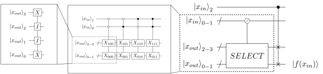
Figure 1: Example of a SelectSwap network with a 3-qubit input and 2-qubit output.

In general, the SelectSwap network requires a T-depth of

$$2^{n-l}+l$$ (1)

and a qubit count of

$$m\times 2^{l}$$ (2)

where $n$ is the number input qubits, $l$ is the number of swap qubits and $m$ is number of qubits required to store the output $f(x)$ in a fixed-point register.

So far we have described our SelectSwap network using inputs and outputs of binary qubit registers. However we would like to abstract the binary qubit regsiter to a fixed-point qubit register. Q# has an in-built fixed point register structure which readily takes care of the conversions between binary and fixed-point qubit registers. That in addition to Q# having some readily available operations in its in-built libraries (e.g. MultiplexOperations) allowed us to implement the fixed-point SelectSwap operation in fewer than 100 lines of code.

II-B Using the fixed-point implementation of a LUT to implement quantum arithmetic functions

The SelectSwap operation from the previous section requires the user to input the number of qubits in the input and output fixed-point register, as well as the binary values of each of the desired outputs. However, to remove the burden of computing these quantities from the user, we created a wrapper function ApplyFunctionWithLookup that contains the above SelectSwap network. This wrapper function requires the user to provide the input domain $(x_{\min},x_{\max})$, maximum allowed input error tolerance $\epsilon_{\mathrm{in}}$, minimum required output precision $\epsilon_{\mathrm{out}}$ and number of swap qubits. Aside from the last one, these are the parameters that practitioners will typically focus on when implementing quantum arithmetic operations within a larger end-to-end algorithm. The last parameter is used to be able to perform the tradeoff between T-count/depth and qubit count (which we discuss in more detail later on).

In addition to returning the the LUT operation object, the wrapper function also returns the number of integer and fractional bits required for the input and output. This is required to create the fixed-point registers that the LUT operation will use as input and output qubit registers. We present the pseudocode of the wrapper function in Algorithm 1. We note that we require the subtraction circuit in Step 3 whenever $x_{\min}\neq 0$ because the LUT is designed in such a way that its list of outputs $\left(f(\hat{x}_{0}),f(\hat{x}_{1}),\dots\right)$ corresponds to inputs in order from $00\dots 0$ to $11\dots 1$, so the implementation performs the subtraction to have the minimum value $\hat{x}_{0}$ be represented by $00\dots 00$, the next value $\hat{x}_{1}$ be represented by $00\dots 01$ and so on.

Algorithm 1 The wrapper function ApplyFunctionWithLookup that implements the quantum LUT for arithmetic operations

1:Inputs

2:$f(\cdot)$: Desired arithmetic function to implement

3:$(x_{\min},x_{\max})$: Input domain (with inclusive bounds)

4:$(\epsilon_{\mathrm{in}},\epsilon_{\mathrm{out}})$: Maximum allowed error for the input value and precision tolerance for the output value

5:$l$: Number of qubits to be used as swap qubits

6:Outputs

7:LUT: Lookup table Q# operation

8:$(n,p)$: Number of total bits and integer bits respectively required for the input fixed-point register to the LUT

9:$(m,q)$: Number of total bits and integer bits respectively required for the output fixed-point register of the LUT

10:procedure ApplyFunctionWithLookupabcdefghijklmno ($f(\cdot),(x_{\min},x_{\max}),(\epsilon_{\mathrm{in}},\epsilon_{\mathrm{out}}),l$)

1. Compute the list of inputs $\hat{x}_{i}$ in fixed point representation as well as $(n,p)$ given $(x_{\min},x_{\max})$ and $\epsilon_{\mathrm{in}}$

2. Using the inputs $\hat{x}_{i}$, compute the list of outputs $\hat{f}(\hat{x}_{i})$, the approximation of $f(\hat{x}_{i})$ in fixed-point representation to within a precision of $\epsilon_{\mathrm{out}}$, and $(m,q)$

3. If $x_{\min}\neq 0$, create a Subtraction circuit that takes in a fixed-point register and subtracts $x_{\min}$ from it

4. Create the SelectSwap circuit using $\hat{x}_{i}$, $\hat{f}(\hat{x}_{i})$ and $l$ and append it to the Subtraction circuit

We make use of several Q# library functions that are convenient to design this wrapper function, such as conversion functions BoolArrayAsInt and DoubleAsFixedPoint which easily handle the many transformations from one representation to another which were required throughout the implementation of the wrapper function. A simple example of how to use the ApplyFunctionWithLookup wrapper function to implement an exponential function can be seen in Appendix A.

III Error analysis of the LUT to implement quantum arithmetic functions

The final LUT operator guarantees that given an input value $x$ and an arithmetic function $f(\cdot)$, it will compute $\hat{f}(\hat{x})$ where $\hat{f}$ is an approximation of $f$ to within a precision of $\epsilon_{\mathrm{out}}$, and $\hat{x}$ is an approximation of the input value $x$ to within the maximum allowed input error tolerance $\epsilon_{\mathrm{in}}$. We note that the total output error is composed of $\epsilon_{\mathrm{out}}$ as well as the error propagated by the difference between $\hat{x}$ and $x$. Therefore if the function $f$ is highly oscillatory and/or does not have well-behaved derivatives, then the circuit created to approximate $f(x)$ may lead a high output error. However many commonly used arithmetic operations on well defined domains, including everywhere differentiable functions, are Lipschitz continuous i.e. exhibit the property $|f(\hat{x})-f(x)|\leq L|\hat{x}-x|$ for some constant $L$. Therefore for Lipschitz continuous functions, the total output error given by the LUT implementation is upper bounded by

$$|\hat{f}(\hat{x})-f(x)| =|\hat{f}(\hat{x})-f(\hat{x})+f(\hat{x})-f(x)|$$

$$\leq|\hat{f}(\hat{x})-f(\hat{x})|+|f(\hat{x})-f(x)|$$

$$\leq\epsilon_{\mathrm{out}}+L|\hat{x}-x|$$

$$=\epsilon_{\mathrm{out}}+L\epsilon_{\mathrm{in}}$$ (3)

In the case of everywhere differentiable functions, $L$ can be replaced with $\sup|\frac{df}{dx}|$. Therefore when implementing the LUT, the user can easily compute an upper bound of the total output error and use it to determine the desired $\epsilon_{\mathrm{in}}$ and $\epsilon_{\mathrm{out}}$ input values. Being able to define the total output error explicitly is an important feature of the implementation. Firstly, it allows the user to keep track of the error propagation when using the operator in end-to-end implemenations of quantum algorithms. Secondly, it also makes the LUT implementation a good benchmark for evaluating the efficiency of single variable bespoke quantum arithmetic circuits.

IV Comparing the LUT implementations for quantum arithmetic functions to bespoke implementations

We now compare LUT quantum arithmetic functions with bespoke quantum arithmetic implementations. In particular, we look at three examples: the exponential, Gaussian and square root functions. Given that these arithmetic functions require a large amount of qubits, we look at the resources from a fault-tolerant perspective and assume an architecture using Clifford+T-gates as fundamental operations. In this setting, the resources required to create error-corrected T-gates largely outweigh the resources for creating any Clifford gate [9], which is why we focus on the T-count, T-depth and qubit numbers. We note that Q# has an in-built resource estimation engine that allows for T-count, T-depth and qubit count calculations for any operation. An example of a code snippet used to compute the resources for a LUT implementation can be found in Appendix A.

IV-A Exponential and Gaussian functions

In Table I, we compare the resources for the LUT implementation with the implementation by Poirier for different domains and error tolerances as shown in [10]. In addition to the examples found in [10], we also computed the resources to implement $e^{-x}$ for the domain $[\log(1/2),0]$ since in principle any additional power of $e^{-x}$ can be implemented with a bit shift in the fixed point representation of the input by computing the input mod $\log(1/2)$ and then computing the argument and bit shifting the results down. The details of how the parameters for Table I were deduced from [10] for the Poirier method can be found in Appendix B.

TABLE I: Comparing the T-count and Qubit count of exponential and Gaussian functions between the Poirier method [10] and the LUT implementations. For LUT implementation, we used 0 swap qubits in the $e^{-x}$ computations and 5 swap qubits in the $e^{-x^{2}}$ computations.

$f(x)$	$(x_{\min},x_{\max})$	$(\epsilon_{\mathrm{in}},\epsilon_{\mathrm{out}})$	T-count		Qubit Count
			Poirier	LUT	Poirier	LUT
$e^{-x}$	(0, 10)	$(2^{-3},10^{-7})$	6480	1176	154	36
		$(2^{-4},10^{-9})$	17752	2310	264	45
	(0, 100)	$(1,10^{-7})$	3648	1442	134	30
		$(2^{-1},10^{-9})$	11312	2856	233	42
	($\log(1/2)$, 0)	$(2^{-4},10^{-7})$	6480	574	154	45
		$(2^{-5},10^{-9})$	17752	826	264	57
$e^{-x^{2}}$	(0, 10)	$(2^{-9},10^{-7})$	17872	13560	325	3365
		$(2^{-11},10^{-9})$	33200	36552	465	4143
	(0, 100)	$(2^{-6},10^{-7})$	2816	13560	141	3331
		$(2^{-8},10^{-9})$	12928	36552	262	4119

We notice that the difference between the resources required to compute $e^{-x}$ and $e^{-x^{2}}$ are quite large, even though it would seem that two can be interconverted in a straightforward way by using a squaring circuit before inputing into $e^{-x}$. However a squaring circuit would add its own approximation errors which would need to be rigorously taken into account. This would require splitting the error between the two circuits and making up for any additional errors. Hence the conversion is not so straightforward and could lead to an increase in resources.

We would now like to look more closely at the interesting case of the function $e^{-x^{2}}$ with $(x_{\min},x_{\max})=(0,10)$ and $(\epsilon_{\mathrm{in}},\epsilon_{\mathrm{out}})=(2^{-9},10^{-7})$. We see that there are trade-offs wherein it can be more or less efficient to use the LUT circuit vs the Poirier implementation depending on what you are trying to optimize. Therefore, we use this example to illustrate the demonstrate the T-gate to qubit count trade-offs that can be had when changing the number of swap qubits in the LUT implemention in Figure 2.

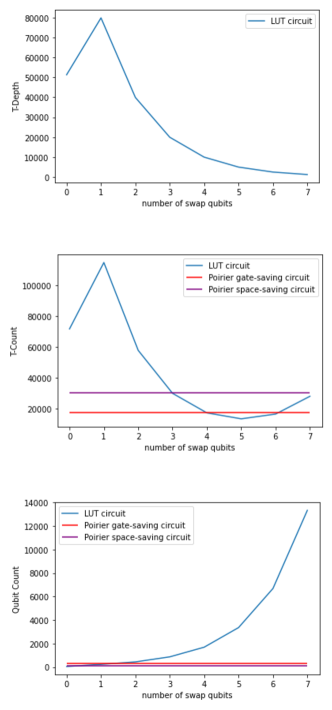
Figure 2: Plots showing resources to implement the LUT for $e^{-x^{2}}$ with $(x_{\min},x_{\max})=(0,10)$ and $(\epsilon_{\mathrm{in}},\epsilon_{\mathrm{out}})=(2^{-9},10^{-7})$.

For this particular case, we see that the Poirier method is clearly much more efficient in terms of qubit numbers. However the LUT implementation has the ability to trade off for lower T-count/depth if there are sufficient qubits available.

IV-B The square root function

In Table II, we compare the resources for the LUT implementation with the ESOP based synthesis [11] implementation and the implementation by Dutta et al. for different domains and error tolerances taken from the results as shown in [12]. The details of how the parameters in Table II were deduced from [12] ESOP based synthesis and Dutta et al. methods can be found in Appendix C.

TABLE II: Comparing the T-count and Qubit count for the square root function between the ESOP based synthesis and Dutta et al. methods [12] and the LUT implementations. For the LUT implementations, in each instance we used the number of swap qubits that optimized for T-count.

$(x_{\min},x_{\max})$	$(\epsilon_{\mathrm{in}},\epsilon_{\mathrm{out}})$	T-count			Qubit Count
		ESOP	Dutta et al.	LUT	ESOP	Dutta et al.	LUT
(0, 4)	$(2^{-5},2^{-5})$	803	27769	1288	16	210	269
(0, 8)	$(2^{-7},2^{-7})$	1746	53011	4216	22	288	1317
	$(2^{-9},2^{-9})$	10242	74319	9576	26	338	3121
(0, 16)	$(2^{-9},2^{-9})$	31075	86317	13664	28	363	3357

Similarly to the results for the exponential and Gaussian functions, we can look at the T-gate to qubit count trade-offs that can be had when changing the number of swap qubits in the LUT implemention for an interesting example. In this case, we will focus on the example with $(x_{\min},x_{\max})=(0,16)$ and $(\epsilon_{\mathrm{in}},\epsilon_{\mathrm{out}})=(2^{-9},10^{-9})$. The results can be seen in Figure 3.

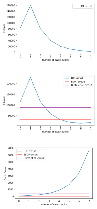
Figure 3: Plots showing resources to implement the LUT for $\sqrt{x}$ with $(x_{\min},x_{\max})=(0,16)$ and $(\epsilon_{\mathrm{in}},\epsilon_{\mathrm{out}})=(2^{-9},2^{-9})$.

Simlarily in this case as well, we notice that the ESOP synthesis based method is clearly much more efficient in terms of qubit numbers, but that LUT implementation has the ability to trade off for lower T-count/depth if there are sufficient qubits available.

IV-C Remarks and general observations

In terms of the performance of the LUT implementation with respect to bespoke implementations, we make a few remarks:

• The LUT implementation is in general comparable to bespoke implementations of arithmetic functions, where the performance being better or worse is dependent on the specific function being implemented. We also find that the LUT function has the ability to trade-off between T-count/depth and qubit count such that it can often outperform bespoke implementations in the former but at a large cost of the latter.

• By characterizing the parameters $(x_{\min},x_{\max})$ and $(\epsilon_{\mathrm{in}},\epsilon_{\mathrm{out}})$ when implementing the function, we were able to make a fair comparison between the LUT implementation and bespoke implementations while also using a benchmark that is relevant to practitioners.

• For the simple operations of comparing to a constant, adding or subtracting a constant [13], and multiplying or dividing by a constant, the current state-of-the-art bespoke methods widely outperform the LUT implementation. This can be seen by noting that the T-counts, T-depths and qubit counts of those operations are linear in the number of input qubits with a small constant factor, which is favorable with respect to Equation 1 and Equation 2.

V Conclusion and Discussion

In this paper, we have presented an implementation of a function that can create a quantum lookup table for any single-variabled arithmetic functions. The implementation only requires the desired function, input domain, allowed error tolerances and number of swap qubits as input, which are the parameters that practitioners will typically focus on when implementing quantum arithmetic operations within a larger end-to-end algorithm. The implementation then takes care of all the appropriate possible outputs for the LUT and the actual LUT operation itself. It will also output the number or required integer and fractional input and output bits such that the user can easily create the required fixed point input and output registers used as arguments to the LUT operation. We then discuss how the approximation error of the operator can be understood. This understanding allows for the implementation to be used in two settings: (1) one can easily use it and keep track of its approximation errors when implementating in end-to-end algorithms and (2) it can be used as a well-defined benchmark for evaluating the efficiency of single variable bespoke quantum arithmetic circuits. Finally, we demonstrated how our implementation can be used to create LUT operations for quantum arithmetic functions, and compared them to state-of-the-art bespoke quantum arithmetic functions using in-built Q# functionalities to compute T-count, T-depth and qubits counts.

As a next step, one can think about implementing a function that, given a desired arithmetic operation, input domain and error tolerances, would automatically compute which between the LUT implementation or the bespoke implementation of said operation is more efficient and return the appropriate operation object with all the required parameters to create the fixed-point registers. One can also think of incorporating a feature that performs linear or more complicated interpolations after the quantum arithmetic operation which may allow for overall lower output errors for the same amount of gate and qubit resources. One can also think of slightly restructing the LUT implementation such that instead of the implementation outputting an operation object with the required parameters to create the appropriate fixed-point registers, the function would encompass an object that would itself handle the creation and propagation of these registers.

Finally, an interesting line of work would be to try and understand more about which general classes of single variable quantum arithmetic functions would we expect LUT implementations to perform better compared to other (e.g. reversible or QFT) implementations.

Appendix A Q# code to implement the LUT in a program

An example of a Q# file using the ApplyFunctionWithLookupTable function to implement the LUT function can be found in the code snippet in Figure 4. The example code below was used to implment the function $e^{-x}$ for $(x_{\min},x_{\max})=(0,10)$, $(\epsilon_{\mathrm{in}},\epsilon_{\mathrm{out}})=(2^{-3},10^{-7})$ and 0 swap qubits.

     namespace ResourceEstimate {      open Microsoft.Quantum.Arithmetic;    open Microsoft.Quantum.Math;      function ExpInv(x: Double) : Double {      return ExpD(-x);    }      @EntryPoint()    operation Main() : Unit {      let xmin = 0.0;      let xmax = 10.0;      let epsin =  PowD(2.0, -3.0);      let epsout = 1e-7;      let numswap = 0;      let lookup = ApplyFunctionWithLookupTable(        ExpInv, (xmin, xmax), epsin, epsout, numswap);      use input = Qubit[lookup::IntegerBitsIn +        lookup::FractionalBitsIn];      use output = Qubit[lookup::IntegerBitsOut +        lookup::FractionalBitsOut];      lookup::Apply(FixedPoint(        lookup::IntegerBitsIn, input),        FixedPoint(lookup::IntegerBitsOut,        output));    }  }     

Figure 4: Code snippet to implement the LUT function in Q#

Once the file is created, the command to run the resource estimator is dotnet run -s ResourcesEstimator. To implement any other single variable arithmetic function (either user-defined or native), the user simply needs to replace ExpInv in the Main operation with the desired function.

Appendix B Deducing the parameters for Table I from [10]

The resources displayed in Table I for the Poirier method were taken from Table II in [10]. The parameters $x_{\min}$, $x_{\max}$, and $\epsilon_{\mathrm{out}}$, as well as the qubit count for the Poirier method are explicitly stated in [10] and were taken directly as is. The parameter $\epsilon_{\mathrm{in}}$ was determined by looking at the number of input qubits $n$ and computing the value represented by the least significant bit given a register representing $x_{\max}$ assuming the register is in a fixed-point binary representation. For example in the case where $0\leq x\leq 10$ with $d=7$ input qubits, we note that the most siignificant bit has to represent at least $2^{3}$, so the least significant bit represents $2^{3-7}=2^{-4}$ which gives us our value for $\epsilon_{\mathrm{in}}$ (we have assumed no sign bit). And finally to compute the T-counts, we multiply the Toffoli counts given in [10] by 4 where we have assumed the efficient implementation of the Toffoli gate using Clifford+T gates given in as [14]. For the $(x_{\min},x_{\max})=(\log(1/2,)0)$ case, we assumed the same register sizes as for $(x_{\min},x_{\max})=(0,10)$ (i.e. $(n,d,m)=(21,7,7)$ for $\epsilon_{\mathrm{out}}=10^{-7}$ and $(n,d,m)=(32,8,8)$ for $\epsilon_{\mathrm{out}}=10^{-9}$) and computed the values for $\epsilon_{\mathrm{in}}$ in the same way as for the other other cases.

Appendix C Deducing the parameters for Table II from [12]

The resources displayed in Table II for the ESOP based synthesis and Dutta et al. methods were taken from Fig 5.a in [12]. All the parameters were taken based on the number of integer and fractional qubits used to represent the input fixed point representation, given by $m$ and $n$ respectively. It was assumed that the output registers also contained $m$ integer qubits and $n$ fractional qubits. So we calculated the domains as $(x_{\min},x_{\max})=(0,2^{m})$ and the errors as $\epsilon_{\mathrm{in}}=\epsilon_{\mathrm{out}}=2^{-n}$. The T-counts and qubit counts were explicitly stated in the table and were used as is in Table II. The precise value of $x_{\max}$ for those results were actually $2^{m-1}+2^{m-2}+\dots+2^{0}+2^{-1}+\dots+2^{-n}$, but we computed the metrics for the LUT implementation using $x_{\max}=2^{m}$, thus giving slightly more conservative results.

References

- [1] S. al-D. al-Tusi, “Treatise on Equations,” 1209.
- [2] L. Euler, “Institutiones Calculi Differentialis,” 1755.
- [3] K. Svore, A. Geller, M. Troyer, J. Azariah, C. Granade, B. Heim, V. Kliuchnikov, M. Mykhailova, A. Paz, and M. Roetteler, “Q#: Enabling Scalable Quantum Computing and Development with a High-level DSL,” Real World Domain Specific Languages Workshop, pp, 7:1–7:10, 2018
- [4] T. Häner, M. Roetteler, and K. M. Svore, “Optimizing Quantum Circuits for Arithmetic,” arXiv:1805.12445, May 2018.
- [5] E. Y. Remez, “Sur la détermination des polynômes d’approximation de degré donnée,” Comm. Soc. Math. Kharkov, vol 10, 41–63, 1934.
- [6] M. Soeken, M. Roetteler, N. Wiebe, and G. De Micheli, “LUT-Based Hierarchical Reversible Logic Synthesis,” IEEE Trans. on CAD vol 38, 1675–1688, July 2018.
- [7] G. Hao Low, V. Kliuchnikov, and Luke Schaeffer, “Trading T-gates for dirty qubits in state preparation and unitary synthesis,” arXiv:1812.00954, December 2018.
- [8] R. Babbush, C. Gidney, D. W. Berry, N. Wiebe, J. McClean, A. Paler, A. Fowler, and H. Neven, “Encoding Electronic Spectra in Quantum Circuits with Linear T Complexity,” Phys. Rev. X, vol. 8, 041015, October 2018.
- [9] E. T. Campbell, B. M. Terhal and C. Vuillot, “Roads towards fault-tolerant universal quantum computation,” Nature vol 549, 172-179, 2017.
- [10] B. Poirier, “Efficient Evaluation of Exponential and Gaussian Functions on a Quantum Computer,” arXiv:2110.05653, October 2021.
- [11] A. Mishchenko and M. Perkowski, “Fast Heuristic Minimization of Exclusive-Sums-of-Products”, 5th International Reed-Muller Workshop, September 2001.
- [12] S. Dutta, Y. Tavva, D. Bhattacharjee and A. Chattopadhyay, “Efficient Quantum Circuits for Square-Root and Inverse Square-Root,” 2020 33rd International Conference on VLSI Design and 2020 19th International Conference on Embedded Systems (VLSID), pp. 55-60, June 2020.
- [13] T. Draper, S. Kutin, E. Rains, and K. Svore, “A logarithmic-depth quantum carry-lookahead adder,” arXiv:quant-ph/0406142v1, June 2004.
- [14] C. Jones “Low-overhead constructions for the fault-tolerant Toffoli gate,” Phys. Rev. A, vol 87, 022328, February 2013.