Binary neutron star merger simulations with neutrino transport and turbulent viscosity: impact of different schemes and grid resolution

Abstract

We present a systematic numerical relativity study of the impact of different treatment of microphysics and grid resolution in binary neutron star mergers. We consider series of simulations at multiple resolutions comparing hydrodynamics, neutrino leakage scheme, leakage augmented with the M0 scheme and the more consistent M1 transport scheme. Additionally, we consider the impact of a sub-grid scheme for turbulent viscosity. We find that viscosity helps to stabilise the remnant against gravitational collapse but grid resolution has a larger impact than microphysics on the remnant’s stability. The gravitational wave (GW) energy correlates with the maximum remnant density, that can be thus inferred from GW observations. M1 simulations shows the emergence of a neutrino trapped gas that locally decreases the temperature a few percent when compared to the other simulation series. This out-of-thermodynamics equilibrium effect does not alter the GW emission at the typical resolutions considered for mergers. Different microphysics treatments impact significantly mass, geometry and composition of the remnant’s disc and ejecta. M1 simulations show systematically larger proton fractions. The different ejecta compositions reflect into the nucleosynthesis yields, that are robust only if both neutrino emission and absorption are simulated. Synthetic kilonova light curves calculated by means of spherically-symmetric radiation-hydrodynamics evolutions up to 15 days post-merger are mostly sensitive to ejecta’s mass and composition; they can be reliably predicted only including the various ejecta components. We conclude that advanced microphysics in combination with resolutions higher than current standards appear essential for robust long-term evolutions and astrophysical predictions.

1 Introduction

The joint observation of the gravitational wave (GW) GW170817 and its associated electromagnetic (EM) counterparts gave the first direct evidence that binary neutron star (BNS) mergers are at the origin of short-gamma-ray burst (SGRB) and kilonova transients (Abbott et al., 2017b, 2019b, a, c; Arcavi et al., 2017; Coulter et al., 2017; Drout et al., 2017; Evans et al., 2017; Hallinan et al., 2017; Kasliwal et al., 2017; Nicholl et al., 2017; Smartt et al., 2017; Soares-Santos et al., 2017; Tanvir et al., 2017; Troja et al., 2017; Mooley et al., 2018; Ghirlanda et al., 2019; Ruan et al., 2018; Lyman et al., 2018). In particular the kilonova counterpart AT2017gfo is commonly interpreted as the UV/optical/infrared transient generated by radioactive decays of $r$-process elements that form in the mass ejected from the merger and the remnant (Chornock et al., 2017; Cowperthwaite et al., 2017; Tanaka et al., 2017; Utsumi et al., 2017; Perego et al., 2017a; Villar et al., 2017; Waxman et al., 2018; Metzger et al., 2018; Kawaguchi et al., 2018; Breschi et al., 2021). In these neutron rich outflows, successive neutron captures produce heavy neutron-rich but unstable nuclei (see, e.g., Cowan et al., 2021; Perego et al., 2021, for recent reviews). The latter decay into stable heavy element nuclei, releasing ${\sim}10^{49-50}$ erg of nuclear energy. The fraction of energy that thermalises inside the ejecta is eventually emitted on a timescale of hours-to-months as the expanding material becomes transparent. A detailed ab-inito calculation of this process is a challenging multi-scale and multi-physics problem that involves extreme gravity, relativistic magnetohydrodynamics (MHD), and advanced microphysics models for the neutron star (NS) matter, including neutrino interactions and transport. Despite recent efforts, complete models of the mass ejecta and the connection to kilonova observations remain very uncertain.

Numerical relativity (NR) simulations represent a fundamental approach for the prediction of astrophysical observables from the merger process and its aftermath (see, e.g., Radice et al., 2020; Bernuzzi, 2020, for recent reviews on the topic). On the one hand, simulations are the only means to calculate GW from the merger and post-merger phase. On the other hand, they crucially allow to identify the different mechanisms for mass ejection together with the kinematical and thermodynamical properties of the unbound material.

Weak interactions and neutrino transport are key ingredients in NR simulations. Neutrinos with energies up to tens of MeV are prominently produced after the collisional shock between the NS cores and, later, in the hottest regions of the merger remnant and accretion disc (see, e.g., Eichler et al., 1989; Ruffert et al., 1997; Rosswog & Liebendoerfer, 2003; Sekiguchi et al., 2011; Perego et al., 2014; Palenzuela et al., 2015; Foucart et al., 2016a; Perego et al., 2019; Endrizzi et al., 2020). Neutrinos emission is the dominant process reponsible for the cooling of the remnant. Electron antineutrinos show the largest peak luminosities, which can reach ${\sim}10^{53}$ erg s^-1 rather independently on the binary parameters (Cusinato et al., 2021). Neutrino-matter interactions determine the composition of the dynamical ejecta primarily via reactions $n+e^{+}\to p+\bar{\nu}_{e}$ and $n+\nu_{e}\to p+e^{-}$. The resulting leptonization process decreases the neutron content in the matter, determining the outcome of the $r$-process nucleosynthesis and the color of the kilonova (Metzger & Fernández, 2014; Martin et al., 2015; Lippuner et al., 2017). Absorption of neutrinos on neutrons affects both the geometry and the mass of the dynamical ejecta, especially at high latitudes (Wanajo et al., 2014; Foucart et al., 2016b; Perego et al., 2017a). Different transport schemes (see below) determine significant differences even in the averaged dynamical ejecta properties (Nedora et al., 2022). Neutrino absorption in the remnant disc drives a wind on timescales of hundreds milliseconds post-merger where lighter nuclei (mass numbers $A\lesssim 130$) are synthesised (Dessart et al., 2009; Perego et al., 2014; Martin et al., 2015; Fujibayashi et al., 2017). This wind may contribute to the early blue kilonova although its mass is not sufficient to explain the peak of AT2017gfo. More ab-initio simulations are required to robutstly determine the mass and other properties of neutrino-driven winds (Nedora et al., 2021b; Fujibayashi et al., 2017). Neutrinos reprocess matter in the density spiral-wave wind that develops from long-lived remnants; this lanthanide-poor material also contributes to a blue transient (Nedora et al., 2019). On seconds timescales, viscosity and neutrino cooling are key processes in the development of disc winds (Fernández et al., 2015; Just et al., 2015; Siegel & Metzger, 2017; Fujibayashi et al., 2018; Radice et al., 2018a; Fernández et al., 2019; Janiuk, 2019; Miller et al., 2019b; Fujibayashi et al., 2020; Just et al., 2021). The latter are poorly explored by NR simulations and using advanced neutrino transport but they are expected to be the main contribution to kilonovae like AT2017gfo (e.g., Radice et al., 2018a; Miller et al., 2019b; Fujibayashi et al., 2020). Neutrinos are also expected to play a role in the (yet uncertain) jet- launching mechanism for SGRB. On the one hand, for small enough jet opening angles, neutrino-antineutrino pair annihilation can deposit the required energy (see, e.g., Eichler et al., 1989; Rosswog & Ramirez-Ruiz, 2002; Dessart et al., 2009; Zalamea & Beloborodov, 2011; Just et al., 2016; Perego et al., 2017b). On the other hand, neutrino absorption in the funnel above the remnant contributes to clean this region from baryon pollution (Mösta et al., 2020).

Neutrino-matter interactions may also impact the high-density regions of the remnant through out-of-equilibrium effects. For example, a trapped neutrino gas can form in the remnant core descreasing the fluid’s pressure (Perego et al., 2019). The analysis of Perego et al. (2019) was performed postprocessing a simulation with leakage (LK)+M0 scheme (see below) and found changes in the pressure at the few percent level. Interestingly, a more recent postprocessing analysis showed that the presence of muons in the remnant NS could affect the trapped neutrino hierarchy and induce variations in the remnant pressure up to $7\%$ (Loffredo et al., 2022). If neutrino trapping occurs, Alford et al. (2018) proposed that modified-Urca processes can lead to bulk viscous dissipation and to damping of the remnant density oscillations. Recently, some authors argued that these out-of-equilibrium effects are present in hydrodynamics and LK simulations and leave a signature in the post-merger GW signal (Most et al., 2022; Hammond et al., 2022). A trapped neutrino gas is observed in the M1 simulations of Radice et al. (2022), but no significant out-of-thermodynamic equilibrium effects on the post-merger dynamics or GW emission were observed. All the simulations employed in these works employ rather low grid resolutions that are known to introduce significant uncertainties in the post-merger dynamics and the GW (e.g., Breschi et al., 2019). Multi-resolution studies employing a consistent neutrino transport and microphysics appear necessary to assess the impact of out-of-equilibrium effects.

The first BNS simulations including neutrino effects employed LK schemes in either newtonian gravity (Ruffert et al., 1997; Rosswog et al., 2003) or general relativity (GR) (Sekiguchi, 2010; Sekiguchi et al., 2011; Neilsen et al., 2014; Galeazzi et al., 2013; Radice et al., 2016). LK schemes do not solve for the equation transport of neutrinos, but rather they parametrise the matter cooling rate due to neutrinos with a phenomenological formula based on the optical depth. Neutrino reabsorption can be simulated by coupling a LK scheme to a truncated multipolar momentum scheme or to ray-tracing algorithms that evolve free-streaming neutrinos in the optically thin regime (Perego et al., 2014; Sekiguchi et al., 2015; Foucart et al., 2015, 2016a; Radice et al., 2016; Fujibayashi et al., 2017; Radice et al., 2018b; Ardevol-Pulpillo et al., 2019; Gizzi et al., 2021). These schemes should be referred to as LK+M0 (or LK+M1). They avoid stiff terms in the hydrodynamics equations and thus they are computationally efficient while capturing the main physical aspects. More advanced transport schemes are based on the full solution of the truncated moment formalism (Thorne, 1981; Shibata et al., 2011). M1 grey schemes for NR simulations of BNS mergers were developed by Foucart et al. (2016b) and more recently refined in Radice et al. (2022), where the complete source terms are implemented. Compared to LK schemes, M1 schemes are believed to better model the optically thick regime on time scales comparable to the cooling timescale although this has not been extensively explored in NR simulations yet. The simulation of dynamical ejecta with the M1 scheme shows less neutron-rich material than the one calculated with LK-based scheme, especially at high latitudes (Foucart et al., 2016b; Radice et al., 2022). The M1 grey scheme has been also compared to a Monte-Carlo scheme on short post-merger timescales to find a few percent agreement on key quantities (Foucart et al., 2020).

MHD instabilities and turbulence are expected to affect the matter flow after merger (Kiuchi et al., 2014, 2015; Kiuchi et al., 2018; de Haas et al., 2022; Combi & Siegel, 2022). They can impact the outcome of the merger and provide crucial processes for the SGRB jet-launching mechanism (e.g. Duez et al., 2004; Duez et al., 2008; Hotokezaka et al., 2013; Ciolfi et al., 2019). Global large-scale magnetic stresses, if they develop, can boost mass ejecta (Metzger et al., 2018; Siegel & Metzger, 2018, 2017; de Haas et al., 2022; Combi & Siegel, 2022). Currently, significant boosts of the mass fluxes can only be achieved by fine-tuning initial configuration or setting unrealistic strength of the magnetic field (Ciolfi, 2020; Mösta et al., 2020). Indeed, one of the main open issues in the simulations is to achieve adequate grid resolution to resolve the amplification of magnetic fields with realistic strenghts and self-consistently obtain turbulent flow (Kiuchi et al., 2018). Sub-grid models have been recently proposed to ease these simulations (Radice, 2017; Shibata & Kiuchi, 2017; Aguilera-Miret et al., 2020). In particular, Radice (2020) proposed a general relativistic Large-Eddy-Simulations (GRLES) calibrated on very high-resoluition GR-MHD resolutions simulations of BNS from Kiuchi et al. (2018).

In this work we perform the first systematic study of the impact of neutrino schemes on the main observables extracted from BNS simulations. We study the evolution of an equal-mass BNS with component masses $1.3~{}{\rm M_{\odot}}$ and a microphysical equation of state (EOS) using hydrodynamics and three different neutrino schemes. We consider a LK, a LK+M0 (hereafter M0) and a M1 scheme. The M0 simulation series is additionally simulated with the GRLES scheme to asses the impact of turbulent viscosity. For each physics prescription, we realise a series of simulations at three different resolutions in order to check convergence and robustness of the results. Our goal is to assess the impact of different microphysics schemes and the role of finite grid resolution on the GW and EM and neutrino emission, and on nucleosynthesis yields.

The rest of the paper is organised as follows. In section §2, we describe our simulations and the different microphysics schemes we use, as well as the simulation’s setup. In section §3, we discuss the evolution of the system, the remnant object and the accretion disc. In section §4 we consider the GW emission and the detectability of effects on the remnant’s core from GW observations. Section §5 is devoted to the study of the dynamical ejecta mass and composition. In section §6 we compare the nucleosynthesis yields and kilonova emission associated to the ejecta from our simulations for different microphysics schemes. In section §7 we examine the variations in neutrino luminosities and average energies comparing M0 and M1 schemes. We summarise and conclude in section §8.

Throughout the text we use latin letters $a,\,b\dots$ as tensor indices, where 0 corresponds to the time index and $1\dots 3$ are the spatial indices. We furthermore use Einstein convention for the sum over repeated indices. We express masses in units of solar masses, ${\rm M_{\odot}}$, and temperature and energy in MeV. The other quantities are reported in SI or cgs units.

2 Methods

2.1 Matter model, initial data and evolution methods

NS matter is modelled using the SLy4-SOR EOS (hereafter SLy), a finite-temperature, composition-dependent EOS based on a Skyrme potential for the nucleonic interaction (Douchin & Haensel, 2001; Schneider et al., 2017). This EOS includes baryons (both free and bound in nuclei), electrons, positrons and photons as the relevant degrees of freedom. The SLy EOS predicts a maximum Tolman-Oppenheimer-Volkoff (TOV) gravitational mass of $M_{\mathrm{max}}^{\mathrm{TOV}}\approx 2.05~{}{\rm M_{\odot}}$ and a radius for a $1.4~{}{\rm M_{\odot}}$ NS of $R_{1.4}\approx 11.9$ km. Both these values are compatible with the observations of extremely massive millisecond pulsars (Cromartie et al., 2019; Fonseca et al., 2021), with results obtained by the NICER collaboration (Miller et al., 2019a; Riley et al., 2019), and with LIGO-Virgo detections (Abbott et al., 2019a); see also Breschi et al. (2021) for a multimessenger analysis based on NR data.

Irrotational initial data in quasi-circular orbit are produced with the pseudo-spectral multi-domain code Lorene (Gourgoulhon et al., 2016). To construct the initial data we use the minimum temperature slice $T=0.01$ MeV of the EOS used for the evolution. Neutrino-less beta-equilibrium is initially assumed inside the two component NSs.

The system is evolved using the 3+1 Z4c free evolution scheme for Einstein’s equations (Bernuzzi & Hilditch, 2010; Hilditch et al., 2013) coupled with the general relativistic hydrodynamics (GRHD) equations. NS matter is modelled as a perfect fluid with stress-energy tensor

$$T_{ab}=(e+p)u_{a}u_{b}+pg_{ab}$$ (1)

where $e$ and $p$ are the energy density and pressure of the fluid, and $u_{a}$ and $g_{ab}$ are the four-velocity and the spacetime metric, respectively. The simulations are performed with the WhiskyTHC  code (Radice & Rezzolla, 2012; Radice et al., 2014b, 2015, a; Radice et al., 2016), which is built on top of the Cactus framework (Goodale et al., 2003; Schnetter et al., 2007). In particular, the spacetime is evolved with the CTGamma code (Reisswig et al., 2013a) which is part of the Einstein Toolkit (Loffler et al., 2012; Ein, ). The time evolution is performed with the method of lines, using fourth-order finite-differencing spatial derivatives for the metric and the strongly-stability preserving third-order Runge-Kutta scheme (Gottlieb & Ketcheson, 2009) as the time integrator. The timestep is set according to the Courant-Friedrich-Lewy (CFL) criterion and the CFL factor is set to $\alpha_{\mathrm{CFL}}=0.15$. Berger-Oliger conservative adaptive mesh refinement (AMR) (Berger & Oliger, 1984) with sub-cycling in time and refluxing is employed (Berger & Colella, 1989; Reisswig et al., 2013b), as provided by the Carpet module of the Einstein Toolkit (Schnetter et al., 2004).

The simulation domain consists of a cube of side ${\sim}3024$ km, centred at the centre of mass of the binary system; only the $z\geq 0$ portion of the domain is simulated and reflection symmetry about the $xy$-plane is used for $z<0$. The grid setup consists of 7 refinement levels centred on the two NSs or in the merger remnant, with the finest level covering entirely each star. In this work we distinguish between low resolution (LR), standard resolution (SR) and high resolution (HR), for which the minimum spacings in the finest refinement level are ${\Delta x}_{\mathrm{LR}}\approx 247$ m, ${\Delta x}_{\mathrm{SR}}\approx 185$ m, ${\Delta x}_{\mathrm{HR}}\approx 123$ m.

In WhiskyTHC  the proton and neutron number densities $n_{p}$ and $n_{n}$ are evolved separately according to

$$\nabla_{a}(J^{a}_{p,n})=R_{p,n}$$ (2)

where $J^{a}_{p,n}\equiv n_{p,n}u^{a}$ is the four-current associated to $n_{p,n}$ and $R_{p}=-R_{n}$ is the net lepton number deposition rate due to absorption and emission of neutrinos and antineutrinos. We denote with $n_{\mathrm{b}}$ the total baryon number density, such that $n_{\mathrm{b}}=n_{p}+n_{n}$ while $Y_{e}$ is the electron fraction, defined as the net number density of electrons and positrons, normalised to $n_{\mathrm{b}}$. Under the assumption of charge neutrality, $n_{p}=Y_{e}n_{\mathrm{b}}$. The expressions for $R_{p,n}$ depend on the particular neutrino treatment employed, which will be discussed in the next subsection.

2.2 Neutrino and turbulent viscosity schemes

Table 1: Weak reactions that are considered in this work. $\nu$ denotes a generic neutrino species amongst electron neutrino $\nu_{e}$, electron antineutrino $\bar{\nu}_{e}$ or heavy flavour neutrinos $\nu_{x}$. The latter is an effective neutrino species containing muon and tau neutrinos and their antineutrinos lumped together. $N$ and $A$ indicate respectively nucleons and generic nuclei.

Reaction	Reference
$\nu_{e}+n\leftrightarrow p+e^{-}$	Bruenn (1985)
$\bar{\nu}_{e}+p\leftrightarrow n+e^{+}$	Bruenn (1985)
$e^{+}+e^{-}\rightarrow\nu+\bar{\nu}$	Ruffert et al. (1997)
$\gamma+\gamma\rightarrow\nu+\bar{\nu}$	Ruffert et al. (1997)
$\nu+N\rightarrow\nu+N$	Ruffert et al. (1997)
$N+N\rightarrow\nu+\bar{\nu}+N+N$	Burrows et al. (2006)
$\nu+A\rightarrow\nu+A$	Shapiro & Teukolsky (1983)

Weak interactions and neutrino radiation are simulated with three different schemes, namely the LK scheme, the M0 scheme (which is always coupled with the LK scheme), and the M1 transport scheme. In all schemes, three different neutrino species are explicitely modelled: $\nu_{e}$, $\bar{\nu}_{e}$, and $\nu_{x}$, where the latter is a collective species describing heavy flavour neutrinos and antineutrinos. Moreover, all schemes are grey, i.e. the explicit dependence on the neutrino energy is integrated out for all the relevant quantities.

The LK scheme (Galeazzi et al., 2013; Radice et al., 2016) accounts for the net emission of neutrinos that are produced as a result of weak interactions happening during and after the NS collision. The reactions that are considered in our simulations are summarised in Tab. 1. Due to the large variety of conditions experienced by matter in BNS mergers, neutrinos that are produced in this process can be roughly divided in two components. A first component gets trapped in the high-density and optically thick regions of the NS remnant, with the possibility of diffusing out on the diffusion timescale. Such component is close to thermodynamical and weak equilibrium with matter. A second component streams freely from the low-density, optically thin regions, with a small probability to further interact with the surrounding matter. The LK scheme uses a phenomenological formula to interpolate between the diffusion rate and the production rate, where the former (latter) is the relevant one in optically thick (thin) conditions. The scheme crucially relies on the evaluation of the optical depth inside the computational domain. The resulting effective rates correspond to neutrinos leaving the system, carrying away energy and lepton number. In particular, the particle emission rates correspond to the rates appearing on the right-hand side of Eq. (2), while the total energy emission rate, $Q$, is included in the simulations as a source term in the Euler equations

$$\nabla_{b}T^{ab}=Qu^{a}\,.$$ (3)

For technical details on the numerical schemes employed for the discretization of Eq. (2) and (3) we refer to Radice et al. (2018b). We stress that such a LK scheme catches the essential cooling effect in NS matter provided by the emission of neutrinos. Moreover, it also affects the matter composition by allowing the conversion of neutrons into protons, and viceversa.

However, neutrinos are not explicitly transported and the possible interaction of streaming neutrinos with matter in optically thin condition is neglected. Additionally, no neutrino trapped component is explicitly modelled in it (i.e., neutrino radiation is not included in the stress-energy tensor), since the density of particles and energy of equilibrated neutrinos are used only to compute the diffusion rates. The non-inclusion of a neutrino trapped component in the remnant NS excludes the correct modelling of out-of-equilibrium effects that might manifest due to the transition from a neutrino-less beta equilibrium to a new equilibrium state with the presence of neutrinos. Finally, the formation and presence of a trapped neutrino gas might change the pressure in the remnant and therefore potentially have an impact on its stability (Perego et al., 2019).

The interaction of the free-streaming neutrino component with matter in optically thin conditions can be simulated in WhiskyTHC using the M0 scheme, as described in Radice et al. (2016). The M0 scheme accounts for possible re-absorption of the emitted neutrinos, as computed by the LK scheme, and the consequent change in matter’s composition (i.e., $Y_{e}$) and temperature. In our simulations the M0 scheme is implemented on a spherical grid centred at the centre of the computational grid, with outer radius ${\sim}756$ km.

A more appropriate way to include neutrinos in the simulations is the M1 scheme, which is an approximated approach to neutrino transport that applies to neutrino radiation in all relevant regimes. The Boltzmann equations describing neutrino transport are first cast into a system of 3+1 equations, similar to the hydrodynamics equations, using a moment-based approach (Thorne, 1981; Shibata et al., 2011). These equations are integrated over the neutrino energy and evolved consistently coupled to the matter and spacetime equations. In the M1 scheme, the terms that describe neutrino interactions with matter are included directly in the stress-energy tensor of Einstein equations. In this work we use the module THC_M1  implemented in WhiskyTHC , which was presented in Radice et al. (2022). For this scheme it is necessary to introduce a closure, i.e. an expression for the pressure in terms of the energy and the flux. We adopt the approximate analytic Minerbo closure. The latter is exact in the optically thick limit (matter and radiation in thermodynamic equilibrium) and in the optically thin limit (radiation streaming at the speed of light in the direction of the radiation flux) if the system has some symmetries (slab, spherical). The two limits are then connected by means of the Eddington factor as described in Radice et al. (2022). The weak interactions that we consider in THC_M1  are the same ones included in the LK scheme, listed in Tab. 1. To ensure stable runs with the M1 scheme we make the following choices. Firstly, we set the relative tolerance parameter that is used to solve the implicit timestep in the source term to $10^{-10}$. Secondly, we additionally enforce local thermodynamical equilibrium depending on the equilibration timescale in a specific cell. In particular, if for a given cell the corresponding timestep constains more than $X$ e-foldings of the equilibration time, we assume the neutrinos average energies at equilibrium for the evolution of the neutrinos number densities. This prevents failures of the runs and the development of spurious features in regions of high density and low $Y_{e}$ in the first few ms after collision. The parameter $X$ has been set as $20$ for LR and HR run and as $10$ for the SR run.

For a subset of simulations in which we employ the M0 neutrino scheme, we additionally include an effective treatment to simulate turbulent viscosity with an implementation based on the GRLES method. In particular, we consider the effect of magnetic-induced viscosity, estimated from high-resolution MHD simulations in full GR from Kiuchi et al. (2018), as described in detail in Radice (2020).

2.3 Simulation sample

In this work, we choose the NS component masses and the equation of state in such a way that the merger results in a remnant NS close to black hole (BH) collapse. We aim at finding possible differences due to the microphysics and resolution in the evolution of such border-line case system. To accomplish this, we pick NS component masses of $M_{1}=M_{2}=1.30~{}{\rm M_{\odot}}$, and baryonic masses $M_{1b}=M_{2b}=1.42~{}{\rm M_{\odot}}$. The symmetric mass ratio of the system is $\nu:=M_{1}M_{2}/\left(M_{1}+M_{2}\right)^{2}=0.25$. The initial separation is set to $\sim$45 km. Thus, the BNS system has a total initial gravitational mass $M\approx 2.60~{}{\rm M_{\odot}}$ and initial ADM mass and angular momentum $M_{\mathrm{ADM}}\approx 2.57~{}{\rm M_{\odot}},\,J_{\mathrm{ADM}}\approx 6.82~{}{\rm M_{\odot}}^{2}$, respectively.

Our study is based on a total of 15 evolutions of the same initial data. We consider a pure hydro case, in which only spacetime and hydrodynamics equations are solved, that we label as HY. Preliminary results about these simulations are presented in Appendix B of Breschi et al. (2019). We simulate the binary evolution including the effect of neutrinos using only the LK scheme, the LK scheme coupled with the M0 scheme, and the more advanced M1 scheme. The three different types of simulations are labelled as LK, M0 and M1, respectively. We refer to the simulation in which we employ M0 and viscosity as VM0. Each model is run at the 3 different resolutions defined in §2.1, namely LR, SR, and HR. We refer to a particular run by indicating first the microphysics and then the resolution; for instance M0-SR is the run with M0 scheme at standard resolution. A complete list of all the simulations is reported in the first column of Tab. 2. The simulations are performed for a minimum of $31$ ms (M1-HR) to a maximum of $155$ ms (LK-LR). Some runs in which a BH forms are affected at later time by the numerical instability described in Radice et al. (2022) and thus were not continued. Simulation data are analyzed to a safe evolution time reported in the second column of Tab. 2; no spurious effects are observed until this time.

3 Remnant dynamics

The two NSs revolve for about 6 orbits before colliding within ${\sim}14$ ms from the beginning of the simulation. The moment of merger is conventionally defined as the peak amplitude of the (2,2) GW mode, and we label it as $t_{\mathrm{merg}}$. The evolution before this moment is referred as the inspiral-merger phase, while the evolution after $t_{\mathrm{merg}}$ is called post-merger. After merger a remnant NS forms, which survives for at least a few tens of ms. In six of our simulations the remnant NS collapses to a BH at $t-t_{\mathrm{merg}}\gtrsim 19.9$ ms.

3.1 Remnant evolution

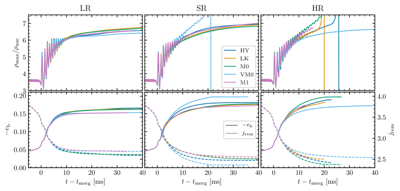
Figure 1: Time evolution of the main quantities describing the dynamics of the system. Top row: maximum rest-mass density in units of the nuclear saturation density $\rho_{\mathrm{nuc}}\approx 2.3\times 10^{14}~{}\mathrm{g~{}cm^{-3}}$. Bottom row: minus the reduced binding energy of the system (solid lines), where $e_{b}:=(M_{\mathrm{ADM}}-E_{\text{GW}}-M)/(M\nu)$; reduced angular momentum of the system (dashed lines), where $j_{\mathrm{rem}}:=(J_{\mathrm{ADM}}-J_{\mathrm{GW}})/(M^{2}\nu)$. $M_{\mathrm{ADM}},\,J_{\mathrm{ADM}}$ are the ADM mass and angular momentum and $E_{\text{GW}},\,J_{\mathrm{GW}}$ are the radiated energy and angular momentum calculated from the multipolar GW (Damour et al., 2012; Bernuzzi et al., 2012b). Time is shifted by the time of merger.

The overall remnant evolution is well described in terms of the maximum rest-mass density, $\rho_{\mathrm{max}}$, (minus) the reduced binding energy, $-e_{b}$, and the reduced angular momentum, $j_{\mathrm{rem}}$, of the system. The latter two quantities are defined as

$$e_{b}:=\frac{M_{\mathrm{ADM}}-E_{\text{GW}}-M}{M\nu}$$ (4)

and

$$j_{\mathrm{rem}}:=\frac{J_{\mathrm{ADM}}-J_{\mathrm{GW}}}{M^{2}\nu}$$ (5)

where $M_{\mathrm{ADM}},\,J_{\mathrm{ADM}}$ are the ADM mass and angular momentum and $E_{\text{GW}},\,J_{\mathrm{GW}}$ are the radiated energy and angular momentum calculated from the multipolar GW (Damour et al., 2012; Bernuzzi et al., 2012b). We report the evolution of these quantities in Fig. 1, comparing the different microphysics in each panel and resolution effects across the three columns.

For $t<t_{\mathrm{merg}}$ the evolution is qualitatively and quantitatively very similar for all the runs. As it can be clearly seen at negative times in Fig. 1, the maximum density (top row), reduced binding energy and angular momentum (bottom row) curves do not display any significant differences across the runs. This is expected, since neutrino production and viscosity effects are negligible in the two NSs. In this regime, increasing the resolution has the only effect of accelerating the merger process and decreasing the time of merger, (see, e.g., Bernuzzi et al., 2012a, b). However, this effect is not visible in Fig. 1, because all quantities are shifted by $t_{\mathrm{merg}}$.

For $t>t_{\mathrm{merg}}$, $\rho_{\mathrm{max}}$ rapidly increases as the NS cores merge reaching $\gtrsim 6~{}\rho_{\mathrm{nuc}}$ within $10$ ms; the damped oscillations are caused by the bounces of the two cores in the process. At about $10$ ms post-merger, the outcome of the GW-dominated (early) post-merger phase is a remnant NS, formed by a core that is slowly rotating surrounded by a rapidly rotating envelope. The absolute value of the binding energy after $t_{\mathrm{merg}}$ measures the compactness of the remnant NS and it increases in time due to the emission of gravitational energy. The bottom row of Fig. 1 shows that most of the emitted gravitational energy and angular momentum are radiated within $t-t_{\mathrm{merg}}\approx 10$ ms (Bernuzzi et al., 2016; Zappa et al., 2018). Comparing to the top row, this period coincides with the time in which the large oscillations of $\rho_{\mathrm{max}}$ are strongly dampened and the remnant NS stabilises or collapses. The physical explanation is that the remnant NS has a large and rapidly evolving quadrupole momentum and is therefore an efficient emitter of gravitational radiation. The emission increases the remnant’s compactness and reduces its angular momentum, thus driving the remnant NS towards axisymmetry and eventually stationarity. Overall, the gravitational energy and angular momentum emission show qualitatively a similar evolution for all the runs. In all cases about the same values of $-e_{\mathrm{b}}\approx 0.12$ and $j_{\mathrm{rem}}\approx 2.9$ are reached at $t-t_{\mathrm{merg}}\approx 5$ ms, and after this time some differences develop among the runs.

Table 2: Main properties of the remnant disc and ejecta for all simulations. The end time of the simulation $t_{\mathrm{end}}$ and of BH collapse $t_{\mathrm{BH}}$ are measured with respect to merger. Disc mass $M_{b}^{\mathrm{disc}}$ and ejecta mass $M_{\mathrm{ej}}$ are baryonic masses and are expressed in solar masses. The ejecta quantities are extracted with the Bernoulli criterion on a spherical surface at $443$ km. The electron fraction $Y_{e}$ and the specific entropy $s$ are reported as mass-weighted averages. The emission angle is calculated as the mass-weighted root mean square (RMS) of the emission latitudes. The analysis is performed until $t-t_{\mathrm{merg}}=20.3$ ms, corresponding to the earliest $t_{\mathrm{end}}$ of our set of simulations, i.e. to the run LK-HR. The only exception is M1-HR, for which we use the last available time $t_{\mathrm{end}}=15.4$ ms post-merger.

Simulation	$t_{\mathrm{end}}$ [ms]	$t_{\mathrm{BH}}$ [ms]	$M^{\mathrm{disk}}_{b}[\mathrm{M}_{\odot}]$		$M_{\mathrm{ej}}[\mathrm{M}_{\odot}]$	$M_{\mathrm{ej}}^{v\geq 0.6c}[\mathrm{M}_{\odot}]$	$\left\langle Y_{e}\right\rangle$	$\theta_{\mathrm{ej}}^{\mathrm{RMS}}[{}^{\circ}]$	$v_{\mathrm{ej,~{}\infty}}/c$	$\left\langle s\right\rangle[k_{\mathrm{B}}/\mathrm{bar}]$
HY-LR	109	-	$1.85\times 10^{-1}$		$1.10\times 10^{-2}$	$1.11\times 10^{-5}$	0.05	34	0.16	16
LK-LR	140	-	$1.76\times 10^{-1}$		$2.41\times 10^{-3}$	$8.60\times 10^{-6}$	0.13	28	0.18	13
M0-LR	94	-	$1.57\times 10^{-1}$		$6.70\times 10^{-3}$	$1.34\times 10^{-5}$	0.23	34	0.16	17
VM0-LR	104	-	$1.80\times 10^{-1}$		$6.44\times 10^{-3}$	$1.48\times 10^{-5}$	0.23	34	0.15	17
M1-LR	35.8	-	$2.42\times 10^{-1}$		$6.59\times 10^{-3}$	$2.02\times 10^{-6}$	0.24	36	0.17	16
HY-SR	109	-	$1.64\times 10^{-1}$		$8.43\times 10^{-3}$	$2.73\times 10^{-5}$	0.049	33	0.19	17
LK-SR	114	-	$8.14\times 10^{-2}$		$2.35\times 10^{-3}$	$1.23\times 10^{-5}$	0.16	30	0.21	14
M0-SR	64.3	64	$7.55\times 10^{-2}$		$5.85\times 10^{-3}$	$3.92\times 10^{-5}$	0.22	32	0.18	16
VM0-SR	35.8	21	$7.58\times 10^{-2}$		$4.02\times 10^{-3}$	$3.09\times 10^{-5}$	0.23	33	0.19	18
M1-SR	41.8	-	$1.51\times 10^{-1}$		$4.13\times 10^{-3}$	$1.29\times 10^{-5}$	0.24	37	0.19	18
HY-HR	27.2	25.6	$1.10\times 10^{-1}$		$7.20\times 10^{-3}$	$2.44\times 10^{-5}$	0.044	34	0.19	18
LK-HR	20.3	19.9	$6.77\times 10^{-2}$		$1.92\times 10^{-3}$	$1.47\times 10^{-6}$	0.17	29	0.2	16
M0-HR	28.6	20.2	$8.98\times 10^{-2}$		$5.11\times 10^{-3}$	$7.96\times 10^{-6}$	0.26	34	0.16	18
VM0-HR	61.3	60.9	$9.46\times 10^{-2}$		$6.14\times 10^{-3}$	$2.80\times 10^{-5}$	0.24	34	0.16	18
M1-HR	15.4	-	$9.29\times 10^{-2}$		$4.09\times 10^{-3}$	$4.43\times 10^{-6}$	0.27	33	0.22	18

During the GW-dominated phase, turbulent viscosity has the largest impact on the remnant’s core dynamics among all the other microphysics prescriptions. In particular $\rho_{\mathrm{max}}$ and $-e_{b}$ in VM0-LR and VM0-HR runs are comparably smaller with respect to the other runs at the same resolution, especially at later times. This effect is due to the fact that viscosity transports angular momentum between the slowly rotating core of the remnant and the rapidly rotating envelope. Consequently, the core can acquire angular momentum at the expenses of the envelope, gaining more rotational support. This effect decreases the central density of the remnant star, making it more stable (Radice, 2017; Shibata et al., 2017a).

The grid resolution has a significant impact on the fate of the remnant. LR simulations present the smallest GW emission, which leads to a less compact and more rotationally supported remnant NS. At LR, gravitational collapse is never observed within the simulated time. At higher resolution, we note overall larger binding energies and smaller remnant angular momenta for all the runs comparing one by one to the LR simulations. For the M0-SR case BH collapse happens at ${\sim}64$ ms post-merger (see third column of Tab. 2), while BH formation is not observed for HY-SR, LK-SR and M1-SR suns within the end of the simulations. The HR simulations show the largest absolute values of binding energies and this determines the largest compactnesses for the remnant stars. As a consequence, we observe BH formation as early as $t-t_{\mathrm{merg}}\approx 20$ ms for LK and M0 runs and $t-t_{\mathrm{merg}}\approx 26$ ms for HY case. In VM0-HR the BH collapse is delayed of about $40$ ms with respect to the other HR runs, due to the viscosity effects described above. The runs that employ M1 transport scheme show a monotonic behaviour with resolution in $\rho_{\mathrm{max}}$, $-e_{b}$, which increase with resolution, while $j_{\mathrm{rem}}$ decreases.

The run VM0-SR has an unexpected behaviour. The remnant NS collapses quite early, around 20 ms post-merger. Comparing to VM0-LR and VM0-HR runs, the density oscillations at $8-10$ ms appear less dampened and $\rho_{\mathrm{max}}$ keeps increasing until the NS eventually collapses. This behaviour has never been observed in previous works where viscosity was included in the same way (Radice, 2020; Bernuzzi et al., 2020). We speculate this result is related to the specific simulation setup that, for this particular BNS, is not yet in a convergent regime at SR. Higher resolution simulations would be required to explore the possibility of obtaining consistent results. We leave this investigation to future work.

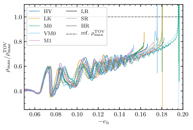
Figure 2: Correlation between the binding energy of the system and the maximum rest-mass density. The latter is rescaled by the central density of the maximum-mass TOV star predicted by the SLy EOS.

Our results highlight that the analysis of the merger dynamics in terms of $\rho$ and energetics is weakly dependent on the particular microphysics setup of the simulations and thus it robustly captures the merger dynamics. This is summarised considering the gauge invariant $\rho_{\mathrm{max}}(-e_{b})$ curves in Fig. 2. The plot shows that the two quantities are clearly correlated, which implies that $\rho_{\mathrm{max}}$ can be, in principle, estimated from a measurement of the total GW radiated energy (Radice et al., 2017). The robustness of the correlation showed in Fig. 2 indicates that our simulations are internally self-consistent among each others. The figure also highlights the fact that in our simulations BH collapse occurs for values of $\rho_{\mathrm{max}}$ below the central density of the maximum-mass TOV star, in particular at values $\rho_{\mathrm{max}}\gtrsim 70\%\rho_{\mathrm{max}}^{\mathrm{TOV}}$ (Perego et al., 2022). This result points to the fact that gravitational collapse is mainly determined by the remnant core, which is slowly rotating and cold.

3.2 Thermodynamic evolution of the remnant

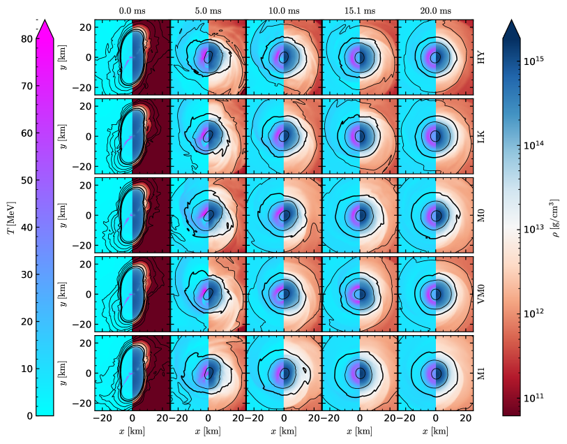
Figure 3: Comparison of the first 20 ms post-merger evolution of the remnant NS for all LR runs. Each row represents a different simulation, while each column corresponds to snapshots taken at the time expressed on top, which refers to $t-t_{\mathrm{merg}}$. The left half of each subplot shows the temperature profile, while the right half shows the density profile in logarithmic scale, both on the equatorial plane. The black contour levels represent iso-density curves. Moving away from the centre, they correspond to decreasing densities of $10^{15},\,10^{14},\,10^{13},\,10^{12}\dots~{}\mathrm{g~{}cm^{-3}}$. The thickest black line has density $10^{13}~{}\mathrm{g~{}cm^{-3}}$ and conventionally denotes the interface between the remnant NS and the disc.

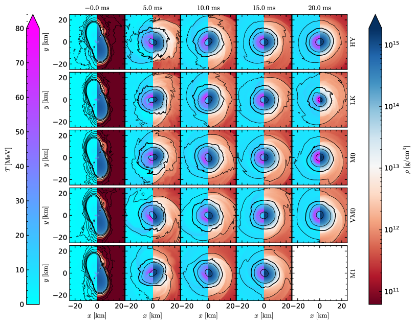
Figure 4: Comparison of the first 20 ms post-merger evolution of the remnant NS for all HR runs. Each row represents a different simulation, while each column corresponds to snapshots taken at the time expressed on top, which refers to $t-t_{\mathrm{merg}}$. The left half of each subplot shows the temperature profile, while the right half shows the density profile in logarithmic scale, both on the equatorial plane. The black contour levels represent iso-density curves. Moving away from the centre, they correspond to decreasing densities of $10^{15},\,10^{14},\,10^{13},\,10^{12}\dots~{}\mathrm{g~{}cm^{-3}}$. The thickest black line has density $10^{13}~{}\mathrm{g~{}cm^{-3}}$ and conventionally denotes the interface between the remnant NS and the disc. The frame corresponding to M1-HR at $t-t_{\mathrm{merg}}=20$ ms is blank because the simulation has a smaller $t_{\mathrm{end}}$.

We now discuss the impact of different neutrino schemes and viscosity on the thermodynamics of the remnant NS.

In Figs. 3 and 4, we report the rest-mass density and temperature profiles on the equatorial plane for LR and HR runs, respectively. For both resolutions, we select snapshots at $t-t_{\mathrm{merg}}=0,5,10,15,20$ ms. The remnant NS is conventionally considered as the region enclosed by the iso-density shell $\rho=10^{13}~{}\mathrm{g~{}cm^{-3}}$, indicated with thick black curves in our plots. Comparing the profiles at LR and HR, the major difference due to resolution is that remnants at HR are more compact; this is in agreement with the binding energy analysis of the system in §3.1. The snapshots $t-t_{\mathrm{merg}}=0$ ms (first column) show the moment in which the two NSs touch and the cores start to fuse, causing the matter at the collisional interface to warm up because part of the kinetic energy is converted into thermal energy. At 5 and 10 ms post-merger (second and third column respectively) the hot matter produced at the collisional interface forms two hotspots at peak temperature $T\approx 70{-}80$ MeV that revolve around the colder core (Kastaun et al., 2016; Hanauske et al., 2017; Perego et al., 2019). At later time $t-t_{\mathrm{merg}}=15$ ms, the hot matter is concentrated in an annulus with a more uniform temperature $T\approx 60-70$ MeV.

The structure of the remnant NS after the GW-phase is almost axisymmetric. The density profile decreases monotonically with the radial coordinates, while the temperature profile does not. In particular, the central densest region of $\rho\gtrsim 10^{15}~{}\mathrm{g~{}cm^{-3}}$ is characterised by $T\lesssim 20$ MeV. In the region of densities $\rho\in[10^{14},\,10^{15}]~{}\mathrm{g~{}cm^{-3}}$ the temperature first increases up to $T\approx 60-70$ MeV and then it decreases down to $T\approx 20$ MeV. The layer of density $\rho\in[10^{13},\,10^{14}]~{}\mathrm{g~{}cm^{-3}}$ is colder, with temperatures $T\lesssim 20$ MeV.

With the exception of the M1 runs, which we discuss below, we do not see any signficant differences in the remnant density profiles comparing runs with different microphysics at the same resolution, as expected. The inclusion of neutrinos emission with LK scheme does not impact significantly the thermodynamics of the remnant’s core, where matter is at high density. Adding neutrino reabsorption with M0 scheme also does not affect the remnant appreciably, because the component of trapped neutrinos is neglected and because free-streaming neutrinos mostly interact with the lower-density material around the remnant NS. The inclusion of turbulent viscosity is also not expected to have a strong impact on the thermodynamics of the remnant core, because the effects of the viscosity model implemented here are by construction small at densities higher than $10^{13}~{}\mathrm{g~{}cm^{-3}}$ (Radice, 2020). In particular, we do not see here an increase in the core temperature due to kinetic energy being converted into thermal energy enhanced by viscosity.

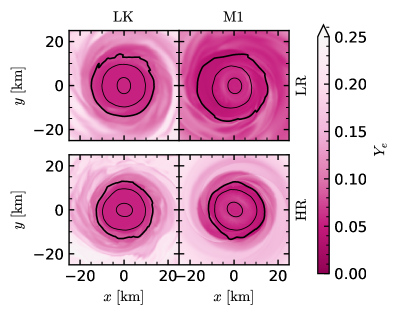
Figure 5: Comparison of $Y_{e}$ inside the remnant between LK and M1 in a 2D snapshot at $t-t_{\mathrm{merg}}=15$ ms on the equatorial plane. The black contour levels represent iso-density curves. Moving away from the centre, they correspond to decreasing densities of $10^{15},\,10^{14},\,10^{13}~{}\mathrm{g~{}cm^{-3}}$. The thickest black line has density $10^{13}~{}\mathrm{g~{}cm^{-3}}$ and conventionally denotes the interface between the remnant NS and the disc. The remnant of the runs with M1 shows an annulus of higher $Y_{e}$ with respect to the LK runs at densities $\rho\in[10^{14},\,10^{15}]~{}\mathrm{g~{}cm^{-3}}$, corresponding to the hot annuli of matter in Figs. 3 and 4.

A comparison of the internal temperature of the remnant star between the runs with LK and M1 at 15 ms post-merger reveals an effect due to neutrino radiation in optically thick conditions. The hot annulus at densities $\rho\in[10^{14},\,10^{15}]~{}\mathrm{g~{}cm^{-3}}$ shows lower temperatures in the M1 run compared to the LK case, with $T^{\mathrm{peak}}_{\mathrm{M1}}\approx 88\%~{}T^{\mathrm{peak}}_{\mathrm{LK}}$. This temperature difference is a physical effect due to the emergence of a neutrino trapped gas that converts fluid thermal energy into radiation energy (Perego et al., 2019).

In Fig. 5 we see the effect in the matter composition of the remnant’s core. In particular we focus on the region $\rho\in[10^{14},\,10^{15}]~{}\mathrm{g~{}cm^{-3}}$ corresponding to the hot annulus of matter. While in LK runs the remnant core retains its pristine $Y_{e}$ with peaks of $Y_{e}\approx 0.058-0.059$, in M1 runs we report that locally $Y_{e}$ can be $40\%$ larger than these values. These variations are consistent for both LR and HR resolutions and with Fig. 9 of Perego et al. (2019). The analysis of Perego et al. (2019) was performed in postprocessing from simulations without the neutrino trapped component, finding that the presence of a neutrino gas would cause a ${\sim}33\%$ increase in $Y_{e}$. Here we confirm this effect in simulations that do simulate the neutrino trapped component inside the remnant (see also Radice et al., 2022).

Figure 6 shows that the thermodynamical conditions inside the remnant is such that locally, in the high-temperature region, the neutrino fractions follow the hierarchy $Y_{\nu_{e}}<Y_{\nu_{x}}<Y_{\bar{\nu}_{e}}$ (Foucart et al., 2016a; Perego et al., 2019; Radice et al., 2022). This is confirmed for all resolutions and it is explained as follows. The matter constituting the hot annulus is characterised by densities $\rho\gtrsim 10^{14}~{}\mathrm{g~{}cm^{-3}}$ and temperatures of few tens of MeV. This is matter initially in cold, neutrino-less weak equilibrium coming from the collisional interface of the fusing NS cores that both decompresses and heats up. Electrons in these conditions are highly degenerate and relativistic, and their chemical potential ($\mu_{e}$) is weakly sensitive to density and temperature variations. On the other hand, neutrons and even more protons are non-degenerate, since their Fermi temperature $T_{\mathrm{F}}$ is such that $T\gtrsim T_{\mathrm{F}}$ and $Y_{p}\sim 0.1Y_{n}$ due to the initial neutron richness. The chemical potentials of protons ($\mu_{p}$) and of neutrons ($\mu_{n}$) are negative, but the absolute value of the former increases faster than the one of the latter. Then, the chemical potential of neutrinos at equilibrium, $\mu_{\nu_{e,{\rm eq}}}=\mu_{p}-\mu_{n}+\mu_{e}$, becomes negative and in particular $-\mu_{\nu_{e,{\rm eq}}}\approx 120$ MeV. For thermalised neutrinos in weak equilibrium, $\mu_{\bar{\nu}_{e}}=-\mu_{\nu_{e}}$ and $Y_{\nu}\propto TF_{2}(\mu_{\nu}/T)$, where $F_{2}(x)$ is the Fermi function of order 2, so that $Y_{\nu_{e}}<Y_{\bar{\nu}_{e}}$. Electron antineutrinos form a mildly degenerate Fermi gas, because the temperature is high and the degeneracy parameter $\eta_{\bar{\nu}_{e}}=\mu_{\bar{\nu}_{e}}/T\approx 2.5-2.7$. Therefore, while electron neutrinos production is suppressed due to the higher neutron degeneracy, electron antineutrinos production is not and a gas of $\bar{\nu}_{e}$ forms, with $Y_{\bar{\nu}_{e}}$ reaching peaks of ${\sim}0.04$. In comparison, the maximum of $Y_{\nu_{e}}$ is of the order of $10^{-3}$, while we find $\max{(Y_{\nu_{x}})}\approx 0.035-0.039$ depending on the resolution. This means that locally each neutrino species constituting the effective species $x$ can be, on average, a factor 4 less abundant than electron antineutrinos.

3.3 Disc evolution

After merger, part of the matter expelled during the collision forms an accretion disc around the remnant object. The baryonic mass of the disc $M_{b}^{\mathrm{disc}}$ is computed from the simulations as the volume integral of the conserved rest-mass density

$$M_{b}^{\mathrm{disc}}=\int_{V}W\rho\sqrt{\gamma}d^{3}x,$$ (6)

where $W$ and $\gamma$ are the Lorentz factor between a fluid element and the Eulerian observer, and the determinant of the spatial three metric, respectively. In our analysis we define the disc as the baryon matter with density lower than $10^{13}~{}\mathrm{g~{}cm^{-3}}$, as in Shibata et al. (2017b). Therefore, the integration domain $V$ extends to all the computational domain excluding the points inside the NS, i.e. the region $\rho<10^{13}~{}\mathrm{g~{}cm^{-3}}$ if a massive NS is present. If a BH forms, the domain is instead restricted by excluding the points inside the apparent horizon using the minimum lapse criterion, i.e. retaining only points for which $\min\alpha\geq 0.3$ (see the discussion in appendix of Bernuzzi et al., 2020, for this choice). $M_{b}^{\mathrm{disc}}$ for all runs are listed in the fourth column of Tab. 2.

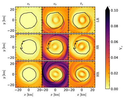
Figure 6: Neutrino fraction inside the remnant for the M1 simulations at $t-t_{\mathrm{merg}}=15$ ms. Each column corresponds to the fraction of one of the three species simulated, while each row corresponds to a different resolution. Inside the remnant the neutrino production is favored for the species $\bar{\nu}_{e}$ and disfavored for $\nu_{e}$. This finding is robust against the resolution employed.

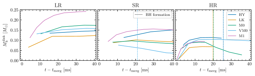
Figure 7: Time evolution of the disc mass comparing all runs at low, standard and high resolution. The vertical dashed lines mark the time of BH collapse. Time is shifted by the time of merger.

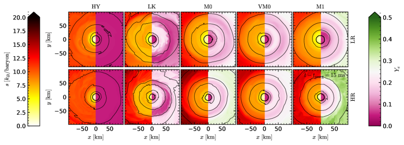
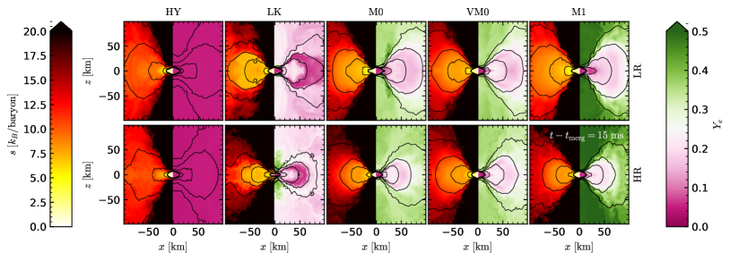
Figure 8: 2D snapshots of the $xy$-plane (top plot) and of the $xz$-plane (bottom plot) showing the properties of the accretion disc around the NS remnant at $t-t_{\mathrm{merg}}=20$ ms. In each plot we compare all runs at LR (top row) to all runs at HR (bottom row). Each frame shows the matter specific entropy $s$ on the left half and the electron fraction on the right half. The thickest black curve is the isodensity contour $\rho=10^{13}~{}\mathrm{g~{}cm^{-3}}$ delimiting the NS remnant, while the other thinner curves moving outwards correspond to densities $\rho=10^{12},\,10^{11},\,10^{10},\dots~{}\mathrm{g~{}cm^{-3}}$. Note that the profiles for M1-HR run are reported at 15 ms post-merger, close to the last available time.

In Fig. 7 we report the first 40 ms post-merger time evolution of $M_{b}^{\mathrm{disc}}$. The largest increase in the disc mass happens within ${\sim}10$ ms post-merger, as a result of the collision and of the successive bounces of the two merging cores. On this timescale the mass of the disc reaches values of the order of ${\sim}0.1~{}{\rm M_{\odot}}$, and then it stays constant for a few tens of ms, if the remnant NS does not collapse. When a BH forms, the disc mass drastically drops because a large fraction of the disc is swallowed by the BH.

To discuss the differences due to microphysics we focus on HR runs. In HY-HR, when neutrinos are not simulated, the disc mass is the largest, being almost double the LK-HR one. Even before BH formation, LK run exhibits the smallest disc mass among all the runs, with $M_{b}^{\mathrm{disc}}\approx 0.06\,{\rm M_{\odot}}$. This can be explained by the fact that LK cools down the lower-density matter around the NS core, causing the outer shells of the remnant NS to be less inflated and to expell less matter. When neutrino reabsorption is present (M0-HR, M1-HR) the disc mass increases to $M_{b}^{\mathrm{disc}}\approx 0.09\,{\rm M_{\odot}}$ and is very similar among the two runs. For VM0-HR, angular momentum and matter transport enhanced by viscosity has the effect of increasing the disc mass with respect to M0 only. Eventually $M_{b}^{\mathrm{disc}}$ reaches an intermediate value between HY-HR and M0-HR ones.

We observe a systematic dependence on resolution in the amount of disc mass. LR runs present the largest $M_{b}^{\mathrm{disc}}$ for all simulations. Here, the minimum mass is found for LK-LR run, with ${\sim}0.12~{}{\rm M_{\odot}}$, while in M0-LR, VM0-LR and HY-LR runs $M_{b}^{\mathrm{disc}}$ reaches similar masses ${\sim}0.15,\,{\rm M_{\odot}}$. The largest disc mass is obtained for M1-LR simulation, with almost ${\sim}0.25\,{\rm M_{\odot}}$. For this resolution a stable rotating NS forms and we also observe that the disc mass slowly increases with time on timescales longer than the ones shown in the plot. This is due to the fact that some matter is explled from the outer shell of the remnant NS and becomes part of the disc (Radice et al., 2018a). For increasing resolution the disc mass decreases comparing each run with its lower resolution counterparts, except for HY-SR. The decrease can be as large as $44\%$ (M0-LR vs. M0-SR). HR runs show the smallest $M_{b}^{\mathrm{disc}}$.

Finite resolution also impact the disc mass indirectly by determining different collapse times. Higher resolution simulations can predict final disc masses that are much smaller than lower resolution ones when a BH forms and it swallows part of the disc. The presence of such lighter discs due to BH collapse can have a large impact on the emission of gravitationally unbound material from the disc at secular timescales (see, e.g., Camilletti et al., 2022; Radice et al., 2018b). We note however that, as long as gravitational collapse does not occur, the spread of $M_{b}^{\mathrm{disc}}$ due to different microphysics is smaller as the resolution increases.

In Fig. 8 we compare the geometric properties and the composition of the disc among the LR and HR runs as 2D snapshots of the $xy$-plane (top plot) and $xz$-plane (bottom plot) at $t-t_{\mathrm{merg}}=20$ ms. The geometry of the disc can be analysed by means of the black iso-density contours in the figure. The high-density portion of the disc $\rho\in[10^{12},\,10^{13}]\,\mathrm{g~{}cm^{-3}}$ extends to ${\sim}20$ km in the equatorial plane and ${\sim}10$ km in the $xz$-plane. The region $\rho\in[10^{11},\,10^{12}]~{}\mathrm{g~{}cm^{-3}}$ is more inflated when neutrinos are present, compared to the HY case, in both $xy$- and $xz$- planes. The low-density $\rho\approx 10^{10}~{}\mathrm{g~{}cm^{-3}}$ tails of the disc extends up to tens of km from the central object on the equatorial plane.

The most evident difference among resolutions is that discs are geometrically smaller for higher resolutions. If we consider the iso-density curve $\rho=10^{10}~{}\mathrm{g~{}cm^{-3}}$ on the orbital plane, it extends to ${\sim}90$ km for LK-LR and ${\sim}65$ km for LK-HR. Similar numbers are found for M0 runs, while in VM0 runs the difference between LR and HR is smaller, ${\sim}10$ km. The largest difference is found in M1 runs, for which the curve extends to $\gtrsim 100$ km for LR and to ${\sim}65$ km at HR.

For the composition of the disc we refer to the the entropy and electron fraction profiles in Fig. 8. The high-density matter $\rho\in[10^{12},\,10^{13}]\,\mathrm{g~{}cm^{-3}}$ is characterised by low electron fraction and low entropy because it is made of fresh matter expelled from the remnant NS. In the HY runs the electron fraction is frozen at $Y_{e}=0.05$ because neutrinos are not simulated. Comparing HY (left column) in the bottom plot with the others, we note that the presence of neutrinos clears the polar regions above the remnant NS (Radice et al., 2016; Mösta et al., 2020). In the runs with neutrinos, at this density, we see that $Y_{e}$ increases up to values $\gtrsim 0.2$ which indicates that matter protonises. In LK runs, for decreasing density and increasing distance from the remnant the $Y_{e}$ first increases as mentioned above, then decreases to $\sim 0.1$ at $\rho\in[10^{10},\,10^{11}]~{}\mathrm{g~{}cm^{-3}}$. At lower densities and high latitude $Y_{e}\lesssim 0.25$. We note that in the region right above the remnant $Y_{e}\approx 0.4$, at LR. At HR the remnant is close to BH collapse and this causes a temperature increase and consequently an increase of electron fraction in the low-density matter above the remnant. The M0 and VM0 runs show different disc composition with respect to LK but similar between each others. Here, a fraction of neutrinos streaming out of the NS remnant is absorbed by lower-density material, increasing its $Y_{e}$. $Y_{e}$ in the shell $\rho\in[10^{10},\,10^{11}]~{}\mathrm{g~{}cm^{-3}}$ is larger than in the LK case at the same density. For increasing latitudes (and decreasing density) $Y_{e}$ increases, reaching values up to $Y_{e}\approx 0.35$. In the M1 runs the electron fraction has larger values when comparing shells of same density to M0 or VM0. In particular matter at high latitude and low density reaches $Y_{e}\approx 0.5$, and is thus quantitative different from M0 runs. The features described are robust against resolution changes.

4 Gravitational waves

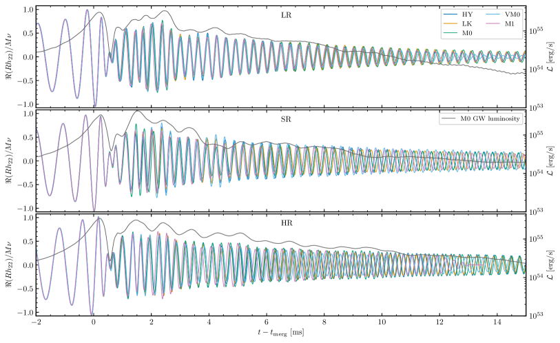
Figure 9: Real part of the $(\ell,\,m)=(2,\,2)$ mode of the GW strain normalised by the total mass of the system $M$, the symmetric mass ratio $\nu:=M_{1}M_{2}/(M_{1}+M_{2})^{2}$ and the extraction radius $R$. The grey curve corresponds to one representative GW luminosity curve (we choose here the M0 runs). Time is shifted by the merger time.

We now compare the GWs emitted during the BNS merger in our simulations. The modes of the gravitational wave strain $h_{\ell m}$ are computed from the Weyl scalar $\Psi_{4}$ projected on coordinate spheres and decomposed in $s=-2$ spin weighted spherical harmonics, $\psi_{\ell m}$. We solve

$$\psi_{\ell m}=\ddot{h}_{\ell m}\,,$$ (7)

using the method of Reisswig & Pollney (2011); the strain is then given by the mode-sum:

$$R\left(h_{+}-ih_{\times}\right)=\sum_{\ell=2}^{\infty}\sum_{m=-\ell}^{\ell}h_{\ell m}(t)\;{}_{-2}Y_{\ell m}(\vartheta,\varphi)\,.$$ (8)

where $R$ is the finite extraction radius in our simulations. Following the convention of the LIGO algorithms library (LIGO Scientific Collaboration, 2018; Cutler & Flanagan, 1994), we let

$$Rh{}_{\ell m}=A{}_{\ell m}\exp(-i\phi{}_{\ell m}),$$ (9)

and compute the gravitational-wave frequency as $\omega{}_{\ell m}=d\phi{}_{\ell m}/dt$, $f_{\ell m}=\omega{}_{\ell m}/2\pi$. In Fig. 9 we compare the $(2,\,2)-$ mode of the GWs among our runs up to 16 ms post-merger. We additionally report the GW luminosity $\mathcal{L}_{\mathrm{GW}}:=dE_{\mathrm{GW}}/dt$ for one representative run (M0 for every resolution). Up to merger, the waveforms do not show any significant differences among each others. The amplitude peaks at $RA_{22}^{\mathrm{merg}}/M\nu\approx 1.06$ with a merger frequency of $f^{\mathrm{merg}}_{22}\approx 1.9$ kHz. The post-merger spectrum peak frequency is $f_{2}\approx 3.2$ kHz. These three quantities are measured quite robustly from our simulations. At LR, the maximum variations of $A_{22}^{\mathrm{merg}}$, $f^{\mathrm{merg}}_{22}$ and $f_{\mathrm{2}}$ among all the runs are respectively ${\sim}0.3\%$, ${\sim}1.3\%$, ${\sim}2.1\%$. At SR the maximum variations of these quantities are below $0.7\%$. Lastly, for HR runs the maximum variations of $A_{22}^{\mathrm{merg}}$, $f^{\mathrm{merg}}_{22}$ and $f_{2}$ among all the runs are respectively ${\sim}0.38\%$, ${\sim}1.1\%$, ${\sim}2.1\%$. The differences due to finite resolution are instead generally larger. We find maximum differences between SR and HR of ${\sim}1.3\%$ for $A_{22}^{\mathrm{merg}}$, ${\sim}4.1\%$ for $f_{22}^{\mathrm{merg}}$ and ${\sim}2\%$ for $f_{2}$. The GW luminosity peaks shortly after merger at $\mathcal{L}_{\mathrm{GW}}^{\mathrm{peak}}\approx 3.5\times 10^{55}$ erg s^-1, consistently with Zappa et al. (2018). The peak value has a maximum variation of ${\sim}34\%$ among our runs.

In the post-merger waveform we see significant differences in the amplitude, frequency and phase evolution among the runs. We first analyze phase convergence among different resolutions and fixed microphysics prescription, and obtain approximately first order convergence. Then, in order to study the impact of resolution over the different simulated physics, we perform a faithfulness analysis between pairs of waveforms. The faithfulness between two waveforms $h_{1}(t)$ and $h_{2}(t)$ is defined as

$$\mathcal{F}:=\max_{t_{c},\,\phi_{c}}\frac{(h_{1}|h_{2})}{\sqrt{(h_{1}|h_{1})(h_{2}|h_{2})}}$$ (10)

where $t_{c},\,\phi_{c}$ are the time and phase of the waveforms at a reference time, the Wiener inner product is

$$(h_{1}|h_{2}):=4\Re\int\frac{{\tilde{h}_{1}(f)\tilde{h}_{2}^{*}(f)}}{S_{n}(f)}df\,,$$ (11)

the symbol $\sim$ denotes the fourier transform, and $S_{n}(f)$ is the power spectral density of the Einstein Telescope. The unfaithfulness is defined as the complement, $\overline{\mathcal{F}}:=1-\mathcal{F}$. In the context of GW parameter estimation, two waveforms are distinguishable if their faithfulness satisfies the necessary criterion (Damour et al., 2011)

$$\mathcal{F}>1-\frac{\epsilon^{2}}{2\varrho^{2}}\,,$$ (12)

where $\varrho$ is the matched-filtered signal to noise ratio (SNR) and we take $\epsilon^{2}=N$, with $N$ number of intrinsic parameters of the system (Chatziioannou et al., 2017). From the above inequality, the minimum SNR that allows to detect the differences between two waveforms can be estimated as

$$\varrho\approx\sqrt{\frac{N}{2\overline{\mathcal{F}}}}.$$ (13)

We compare all our runs in pairs, in such a way that the two runs in a pair have either the same resolution (e.g. HY-LR and LK-LR) or the same microphysics (e.g. HY-LR and LK-LR), excluding comparisons of the kind HY-LR and LK-SR. At LR, we find a maximum mismatch of $\overline{\mathcal{F}}\approx 0.087$ between HY-LR and M0-LR runs. At SR the mismatches are generally larger and we obtain a maximum value of $\overline{\mathcal{F}}\approx 0.2$ between LK-SR and M1-SR and also between M0-SR and VM0-SR runs. At HR the mismatches are the largest and we obtain a maximum of $\overline{\mathcal{F}}\approx 0.32$ between the VM0-HR and M1-HR runs. Comparing runs at different resolutions, we obtain mismatches of the order of few times $10^{-1}$ in almost all comparisons. The only two exceptions are HY-LR vs. HY-SR and LK-LR vs. LK-SR for which $\overline{\mathcal{F}}$ is few times $10^{-2}$.

Our analysis indicates that possible effects due to microphysics can be detected in the GW signal only in the post-merger. However, GW models used for matched filtering that are informed on NR simulations (Breschi et al., 2019, 2022) at LR would not be accurate enough to detect such effects. In particular, differences due to the simulations’ finite resolution would be dominant in such GW models. At SR and HR, mismatches between waveforms of runs performed with different microphysics are comparable to the ones due to finite resolution. GW templates constructed with these data might be able to distinguish such differences in the signal from $\varrho\gtrsim 4$ (Eq. (13)). Notably, this precision might be sufficient for third generation observations, since differences in the signals due to variations in the EOS at extreme matter densities are potentially observable at post-merger SNR ${\sim}8$ (Breschi et al., 2022).

Our results indicate that simulations at SR or HR are necessary in order to distinguish differences due to microphysics in the remnant. In particular, our high-resolution M1 simulations do not show any evidence for significant out-of-equilibrium and bulk viscosity effects in the waveforms. This is in agreement with the findings of Radice et al. (2022) that were obtained at LR, but it is in constrast with Refs. Most et al. (2022); Hammond et al. (2022). The simulations performed for the latter works do not consider weak interactions or use a LK scheme and are performed at a maximum resolution of 400 m, which is much lower than our LR.

5 Mass ejecta

We analyze the material ejected on dynamical timescales and up to ${\sim}20$ ms post-merger. These ejecta include the full dynamical ejecta component and the early portion of the spiral-wave wind component. The dynamical ejecta is composed of a tidal component originating from tidally unbound NS material and a shocked component originating from the first bounce after the core collision (Radice et al., 2018b). The tidal component is launched mostly across the equatorial plane and is characterised by a low $Y_{e}\approx 0.05-0.15$ and low entropy, $s\lesssim 5~{}k_{\mathrm{B}}~{}\mathrm{baryon}^{-1}$. The shocked component has higher entropy than the tidal component and peak temperature of tens of MeV, which produces large amount of electron-positron pairs with consequent increase of $Y_{e}$ due to positron captures on neutrons. Neutrino irradiation from the remnant can further increase $Y_{e}$ of this ejecta component through absorption on neutrons, especially at high latitudes where neutrino emission is more efficient. The shock-heated ejecta expand over the entire solid angle due to interaction with the tidal ejecta, hydrodynamics shocks and weak interaction, with a preference for the emission on the equatorial plane.

Other mechanisms can unbind material from the disc and they act generally on longer timescales. Spiral-wave winds can originate from non-axisymmetric density waves from the NS remnant  (Nedora et al., 2021b). The remnant’s spiral arms transport angular momentum outwards in the disc and material gets then unbound from the disc edge. On longer timescales disc winds can develop, also powered by neutrino reabsorption (e.g. Dessart et al., 2009; Perego et al., 2014; Just et al., 2015; Fujibayashi et al., 2017; Rosswog & Korobkin, 2022) but our simulations are not sufficiently long to capture this component.

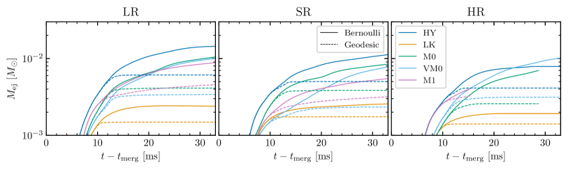
Figure 10: Time evolution of the ejecta mass extracted at $R=443$ km comparing the Bernoulli and geodesic criteria. Mass is reported in logarithmic scale and compared across resolution. Within each subplot we compare the ejecta for all runs.

In the literature there are two main ways to identify the unbound material from simulations, namely the geodesic and the Bernoulli criterion (see, e.g., Foucart et al., 2021, for a recent work on this topic). The geodesic criterion assumes that ejecta follow spacetime geodesics in a time-independent, asymptotically flat spacetime. Therefore, a particle is considered unbound if $u_{t}<-1$, where $u_{t}$ is the time component of the particle’s 4-velocity. According to the Bernoulli criterion, a fluid element is considered unbound if $hu_{t}\leq-1$, where $h$ is the fluid specific enthalpy, $h=1+\epsilon+p/\rho$. Here $\epsilon$ is the specific internal energy, and $p$ and $\rho$ are the pressure and rest-mass density of the fluid, respectively. The asymptotic velocity of the unbound particle is calculated as $v_{\infty}\simeq\sqrt{2\left(h\left(E_{\infty}+1\right)-1\right)}$. This criterion assumes that $hu_{t}$ is constant along a streamline of a steady-state flow. This assumption is correct if the metric and the flow are both stationary. Even though this is not formally true for merger outflows, this criterion is considered sufficient to account for the gain in kinetic energy of the expanding matter in the outflow due to thermal and nuclear binding energy (Foucart et al., 2021). The geodesic and Bernoulli criteria can be used to conventionally identify (separate) the dynamical ejecta from the wind ejecta (Nedora et al., 2021a).

In Fig. 10 we present the evolution of the ejecta mass in our simulations, comparing the geodesic and Bernoulli criteria. At 20 ms post-merger the ejecta masses calculated with the geodesic criterion are saturated, except for the M1 runs. As expected, the ejecta mass calculated with the Bernoulli criterion is larger than the one estimated with the geodesic criterion at comparable times. The ejecta mass in the Bernoulli case keeps increasing at later time due to the contributions of the spiral-wave winds. In the rest of this section we refer to and discuss the Bernoulli ejecta.

The ejecta mass shows a steep increase up to ${\sim}10$ ms post-merger in all the runs and then it tends to saturate at few tens of ms after merger. Within ${\sim}20$ ms post-merger a mass of $\gtrsim 2\times 10^{-3}~{}{\rm M_{\odot}}$ is typically ejected. We refer to Tab. 2 for the quantitative values at a fixed time for all the runs. For HY runs, $\gtrsim 8\times 10^{-3}~{}{\rm M_{\odot}}$ of matter is expelled, which represents the largest matter emission among all the runs. The ejecta mass in LK runs is systematically one order of magnitude lower than that of all the other runs, consistently with Radice et al. (2016). This happens because the neutrino cooling reduces the enthalpy of the material and as a result the emission is largely decreased. When neutrino reabsorption is included through the M0 scheme, the effect of cooling is counteracted by the neutrino energy deposition in the shock-heated ejecta and $M_{\mathrm{ej}}$ becomes larger than the LK case, reaching values $\gtrsim 10^{-2}~{}{\rm M_{\odot}}$. The evolution of $M_{\mathrm{ej}}$ in VM0 runs follows a similar behaviour. $M_{\mathrm{ej}}$ measured in M1 and M0 runs are comparable, within a few tens of percent.

Focusing on the effects of finite resolution, we observe a monotonic decrease of $M_{\mathrm{ej}}$ for increasing resolution for all the runs. Since the onset of BH collapse stops the matter ejection, we measure smaller final ejecta masses in HR simulations than the other cases. Comparing the variations in the ejected mass at a fixed time of 20 ms post-merger due to resolution, we obtain a maximum variation of ${\sim}50\%$ between VM0-SR and VM0-HR.

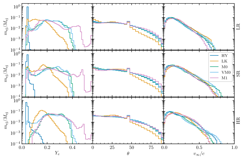
Figure 11: Histograms of the ejecta extracted at $R=443$ km. Each row shows the fraction of ejecta mass in a bin normalised to the total ejecta mass in logarithmic scale for different resolutions. In each columns are represented, respectively, the electron fraction, the latitudinal distribution and the asymptotic velocity of the ejecta. In each frame we compare the ejecta properties among all runs. We perform the analysis until $t-t_{\mathrm{merg}}\approx 20$ ms, corresponding to the earliest $t_{\mathrm{end}}$ of our set of simulations (see Tab. 2). For M1-HR we use the last available time $t_{\mathrm{end}}\approx 15$ ms post-merger.

The most salient properties of the ejected material are summarised in the histograms of Fig. 11. We stress that the histograms produced using the geodesic criterion do not significantly differ from those obtained with the Bernoulli criterion that we show here. In Tab. 2 we report mass-weighted averages of the same quantities presented in the figure. Most of the mass is emitted almost uniformly in the interval $0^{\circ}\leq\theta\lesssim 50^{\circ}$ (second column of Fig. 11). The peak at $\theta\approx 45^{\circ}$ is due to an artefact in the mass extraction and it is not physical. At larger angles, the mass emission is slightly more suppressed in LK runs with respect to the other cases (Radice et al., 2016). The average emission angle for all runs is enclosed in $\theta\in[27^{\circ},\,37^{\circ}]$ and is systematically lower for LK at all resolutions.

The asymptotic velocity distribution is peaked around values in the interval $0.15\leq v_{\infty}/c\lesssim 0.22$. The velocity distribution has fast tails reaching ${\sim}0.8$ c. These tails can originate a radio-X-ray afterglow to the kilonova emission, peaking at years post-merger timescales (Nakar & Piran, 2018; Hotokezaka et al., 2018; Hajela et al., 2022; Nedora et al., 2021a). We measure a mass in the fast tail of the ejecta, i.e. with asymptotic velocity $v_{\infty}/c\geq 0.6$, of ${\sim}10^{-6}-10^{-5}~{}{\rm M_{\odot}}$ (see Tab. 2).

We find that it is possible to model the function $M_{\rm ej}(v_{\infty}/c)$ approximately with a broken power law of the kind

$$M=M_{0}\begin{cases}\left(\frac{\beta\gamma}{(\beta\gamma)_{\beta_{0}}}\right)^{-s_{\mathrm{KN}}}&0.1<\beta\gamma<(\beta\gamma)_{\beta_{0}}\\ \left(\frac{\beta\gamma}{(\beta\gamma)_{\beta_{0}}}\right)^{-s_{\mathrm{ft}}}&\beta\gamma>(\beta\gamma)_{\beta_{0}}\end{cases}$$ (14)

where $\beta=v/c$, $\gamma$ is the corresponding Lorenz factor and $(\beta\gamma)_{\beta_{0}}=\beta_{0}\cdot\gamma(\beta=\beta_{0})$. The values of $\beta_{0}$ defining the “breaks” in the broken power vary in the range ${\sim}0.3-0.45$. Fitting parameters are $M_{0}\approx(3.2-17)\times 10^{-5}~{}{\rm M_{\odot}}$, $s_{\mathrm{KN}}\approx 0.64-1.6$ and the ejecta tail with $v_{\infty}/c\gtrsim\beta_{0}$ can have a rather steep dependence on the velocity, with $s_{\mathrm{ft}}\approx 4-11$.

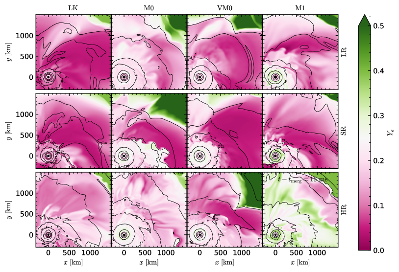
Figure 12: 2D snapshot of the $xz$-plane showing the $Y_{e}$ of the material around the remnant NS at $t-t_{\mathrm{merg}}=20$ ms. The thickest black curve is the isodensity contour $\rho=10^{13}~{}\mathrm{g~{}cm^{-3}}$ delimiting the NS remnant, while the others moving outwards correspond to densities $\rho=10^{12},\,10^{11},\,10^{10},\dots~{}\mathrm{g~{}cm^{-3}}$. Each row correspond to different resolutions, while each column to different micro-physics prescriptions. Profiles for HY runs are not reported because neutrinos are not simulated and the electron fraction distribution is frozen at $Y_{e}=0.05$. Note that the profile for M1-HR run is reported at 15 ms post-merger, close to the last available time.

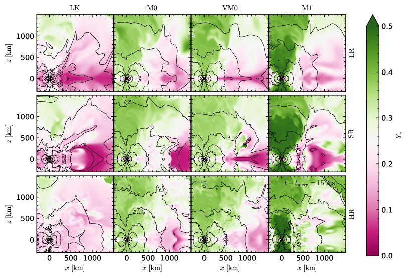
Figure 13: 2D snapshot of the $xz$-plane showing the $Y_{e}$ of the material around the remnant NS at $t-t_{\mathrm{merg}}=20$ ms. The thickest black curve is the isodensity contour $\rho=10^{13}~{}\mathrm{g~{}cm^{-3}}$ delimiting the NS remnant, while the others moving outwards correspond to densities $\rho=10^{12},\,10^{11},\,10^{10},\dots~{}\mathrm{g~{}cm^{-3}}$. Each row correspond to different resolutions, while each column to different micro-physics prescriptions. Profiles for HY runs are not reported because neutrinos are not simulated and the electron fraction distribution is frozen at $Y_{e}=0.05$. Note that the profile for M1-HR run is reported at 15 ms post-merger, close to the last available time.

$Y_{e}$ (first column of Fig. 11) exhibits the most complex behaviours, different among the runs. To discuss it, we also refer in the following to Figs. 12 and 13, where we report 2D slices of the $Y_{e}$ profiles in the $xy$- and $xz$- plane respectively. For HY runs $Y_{e}$ is frozen at ${\sim}$0.05 because weak interactions are not simulated and the matter composition does not change throughout the run with respect to the initial neutrino-less weak equilibrium condition. For LK cases the ejecta mass composition peaks at $Y_{e}\approx 0.13-0.17$ (compare also to Tab. 2). No significant fraction of ejecta has $Y_{e}>0.35$. The material at low $Y_{e}\lesssim 0.15$ is emitted at small latitudes (left-most column of Fig.13), while for increasing angles $Y_{e}$ increases, reaching $Y_{e}\lesssim 0.35$ in the lower-density region above the remnant NS. Matter at high latitudes is shock-heated ejecta, therefore hot, and is expanding in a region where the disc is not present. Under these conditions, the expanding matter becomes transparent earlier producing electron-positron pairs. Therefore, positron captures increasing $Y_{e}$ are more efficient even in absence of neutrino absorption. For both M0 and VM0 the $Y_{e}$ distribution gets broader with respect to LK, with a large fraction of matter having $Y_{e}\in[0.2,0.35]$. This is the effect due to neutrinos radiated by the central object and the disc that are absorbed by neutrons in the ejecta, converting neutrons into protons. As in the previous case, the low-$Y_{e}$ material is emitted at lower latitudes and the $Y_{e}$ increases for increasing latitudes. The peak at $Y_{e}\approx 0.3$ observed in the left column of Fig. 11 is reached in the high-latitudes, low-density ejecta (second and third column of Fig.13). This is because neutrino fluxes are significantly larger at high latitudes, due to the presence of the disc at low latitudes. In M1 runs the trend is similar but even higher values of $Y_{e}$ are reached.

The histograms in Fig. 11 show that the peak at $Y_{e}\approx 0.3$ of M0 and VM0 translates to $Y_{e}\gtrsim 0.425$ when switching to M1. Material with such a high $Y_{e}$ is found once again at large latitudes. The comparison to M0 runs indicates that accounting for neutrino transport with a more complete neutrino scheme provides more efficient proton production in the shock-heated ejecta component. One of the causes of this is that the M0 scheme uses a spherical grid that assumes neutrinos are only moving radially. On the contrary, the M1 scheme is solved in the computational grid and the radiation is evolved according to 3D transport. Neutrinos from the disc will naturally tend to escape along the $z-$ direction, in which the gradient of the optical thickness decreases more steeply and the neutrinos mean-free path increases faster, further irradiating the high-latitude ejecta.

Finite resolution has a clear effect on the ejecta composition, especially visible at HR. All runs at LR and SR show a peak at $Y_{e}\approx 0.05$ that is due to the tidal component of the ejecta, which is emitted at early times after merger and maintains the $Y_{e}$ of the two initial stars. However, for HR runs this component is strongly suppressed for all but the run with viscosity. This can be explained by two different factors. First, the tidal ejecta are expected to be less massive at HR, because the tidal deformation causing this emission at merger are better resolved. Second, the discs are less massive and geometrically thinner for HR runs, compared to the others. Therefore, it is easier for neutrinos to escape from the inner regions and interact with the ejecta, increasing its $Y_{e}$. The latter explanation is supported by the fact that in VM0-HR run the disc is not as thin as in the other HR runs and only for this case the low-$Y_{e}$ peak is not heavily suppressed. This contributes to explain why the M1-HR run exhibits such a large $Y_{e}$ in both the $xy$- and $xz$- planes. On the one hand, the disc is thinner because it is a HR run. On the other hand, neutrino fluxes predicted by the M1 scheme increase the $Y_{e}$ in the matter more efficiently with respect to the M0 scheme.

6 Nucleosynthesis and Kilonova light curves

6.1 Nucleosynthesis

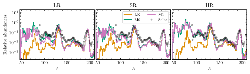
Figure 14: Nucleosynthesis yields comparison between the three physical prescriptions against the solar abundancies for the three resolutions in each panel. On the $x-$axes the mass number $A$ is reported. The relative abundances on the $y-$axis are expressed in logarithmic scale. Consistently with Figs. 11, the analysis is performed up to $t-t_{\mathrm{merg}}\approx 20$ ms for all runs except M1-HR, for which $t-t_{\mathrm{merg}}\approx 15$ ms.

We compute nucleosynthesis abundances inside the ejecta extracted from our simulations according to the procedure described in Radice et al. (2018b). The resulting nucleosynthesis yields are shown in Fig. 16. We compare the results obtained from LK, M0 and M1 runs against the solar residual $r$-process abundances from Arlandini et al. (1999). Abundances are normalised by fixing the overall fraction of elements with $A\in[170,\,200]$ to be the same for all set of abundances. We find that, once the third peak abundaces have been fixed, the abundaces predicted by all neutrinos schemes are roughly compatible among them and with the solar residual pattern for $A\in[125,\,140]$ (i.e., for the second $r$- process peak) and $A\in[170,\,200]$. For $A\in[140,\,170]$ and $A>200$ yields from all of our simulations significantly differ from the solar residuals. Such discrepancies are possibly due to nuclear physics inputs, as well as to a lack of suitable physical conditions to efficiently produce actinides, see e.g. (Mumpower et al., 2017; Wu & Banerjee, 2022). The LK runs heavily underestimate the abundances for $A<120$. This is a direct consequence of the fact that $Y_{e}$ is lower in the ejecta for these cases. In the runs with M0 and M1 the abundances for $A<120$ are closer among them and to the solar residuals, compared to LK.

Increasing the resolution does not change the abundances in runs with LK, which also at high resolution significantly differ from the solar residual abundances for $A<120$. For M0 and especially for M1 runs the predictions at HR better match the solar abundances for the entire range of nuclear masses (still with the exceptions discussed above).

Our results confirm the relevant role of neutrinos emission and absorption in shaping the nucleosynthesis yields from the early time ejecta of BNS mergers (see, e.g., Wanajo et al., 2014; Goriely et al., 2015; Martin et al., 2018; Radice et al., 2018b). Abundances obtained in our HR simulations employing the M0 or M1 schemes are compatible among them and reproduce well the observed solar residual pattern. However, models featuring neutrino cooling alone underestimate the abundances of light $r$-process elements, since neutrino reabsorption is required to produce the ejecta conditions suitable for the production of those elements.

6.2 Kilonova light curves

We compute synthetic kilonova light curves following the approach outlined in Wu et al. (2022) and using the SNEC radiation-hydrodynamics Lagrangian code (Morozova et al., 2015). Accordingly, the dynamical ejecta computed from our simulations are further evolved with SNEC up to 15 days post-merger. The corresponding light curves are presented using the AB magnitude system

$$m_{\mathrm{AB}}=-2.5\log_{10}\left(\frac{\int f_{\nu}(h\nu)^{-1}e(\nu)d\nu}{\int{3631\mathrm{Jy}(h\nu)^{-1}e(\nu)d\nu}}\right)$$ (15)

where here $\nu$ is the light frequency, $f_{\nu}$ is the observed flux density at frequency $\nu$ from a distance of $40$ Mpc and $e(\nu)$ are filter functions for different Gemini bands. We refer to Wu et al. (2022) for more details.

In Fig. 15 we compare the AB magnitudes at different bands to the electromagnetic transient $\mathrm{AT2017gfo}$ associated to the BNS merger event GW170817 (Villar et al., 2017). As input for the SNEC code, we consider the ejecta extracted at two different times: at 20 ms post-merger (dashed lines) and at the end of the simulation (solid lines), with the exception of the HR-M1 run. Clearly, the different simulation lengths impact on the light curve due to the different ejecta masses, but also due to the composition. AT2017gfo is significantly brighter than any of our light curves. Nonetheless the hierarchy of the colors is correct at $\sim$4 days, whereas the 1 day emission has a blue peak that cannot be explained with dynamical ejecta we are considering here. The fact that our analysis does not reproduce the data is expected for many reasons. First, the BNS we simulate is not targeted to the event GW170817; in particular it has lower mass and symmetric mass ratio, which implies smaller ejecta masses and therefore dimmer light curves. Second, our simulations are too short and cannot capture the full evolution of the post-merger disc. Therefore, ejecta emitted at secular timescales (seconds after merger) is missing. Crude estimates of later outflows emission can be made by extrapolating in time (Wu et al., 2022), but we do not attempt this here. Third, multidimensional effects and viewing angle can have a strong impact on the kilonova emission (e.g., Perego et al., 2017a; Kawaguchi et al., 2020; Korobkin et al., 2020) but are neglected here. For AT2017gfo, spherically symmetric kilonova models are ruled out with high confidence (Villar et al., 2017; Perego et al., 2017a; Breschi et al., 2021). In the following we focus on the differences seen for different microphysics.

For HY runs we obtain that light curves corresponding to the $K_{s}$, $H$ and $J$ band are only a few magnitude larger than AT2017gfo data, especially when we consider ejecta production at ${\sim}109$ ms post-merger (solid lines in the LR and SR cases). By contrast, dynamical ejecta alone produce significantly dimmer light curves (dashed lines), in particular at late time after the peaks. Despite the usually long simulation lengths, for LK runs the ejecta mass is smaller and this produces dimmer light curves compared to HY runs, considering both the early ejecta and those at the end of the simulations. The jumps that we observe in these curves are an artefact of the SNEC code. For M0, VM0 and M1 we obtain brighter light curves at all bands with respect to LK, as a consequence of the fact that more ejecta mass, characterised by a larger $Y_{e}$, is produced. When considering only the early ejecta (dashed lines), M0, VM0 and M1 produce very compatible light curves, due to the very similar ejecta properties, see Sec. 5 and Table (2). M1 light curves are slightly dimmer due to the faster and less opaque ejecta, which translate in a faster kilonova evolution after the peaks. Differences become more pronounced when light curves are computed using the ejecta at the end of the simulations, since M1 runs were evolved for shorter post-merger times and produced systematically less ejecta mass.

Finite resolution does not significantly impact the light curves. Our analysis shows that the light curves are very sensitive both to the inclusion of neutrino reabsorption in optically thin conditions and to the cumulative time during which ejecta are measured. During this time not only the ejecta mass, but also the ejecta composition changes due to the different emission mechanisms at different timescales. The better accuracy provided by the M1 scheme with respect to the M0 one seems to have a minor impact on the kilonova light curves due to the good agreement in the ejecta properites between the two schemes, when the simulations have comparable lengths. Future simulations will extend these results by also considering the winds from the viscous post-merger phase and taking into account non-spherical geometries.

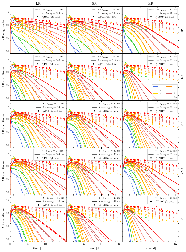
Figure 15: Light curves calculated with SNEC. We report the AB magnitudes as a function of days after merger. The light curves corresponds to several Gemini bands and are calculated from the ejecta extracted at $R=443$ km from the system at a common time $20$ ms post-merger (dashed lines) and at the end time of each simulation (solid lines). Dots correspond to the data of the kilonova event AT2017gfo for the same bands.

7 Neutrino luminosity

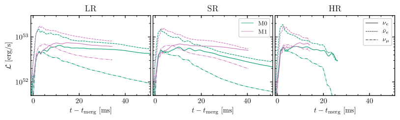
Figure 16: Neutrino luminosity comparison between M0 and M1 simulations for all three neutrino species and for the three resolutions in each panel. Neutrinos are extracted at a radius $R_{\mathrm{M0}}=756$ km for the M0 case and $R_{\mathrm{M1}}=443$ km for the M1 case. The data is smoothed using a rolling average with width 1 ms. Time is shifted by the time of merger and by the time of flight of neutrinos to the corresponding detector. The luminosity is expressed in cgs units and in logarithmic scale.

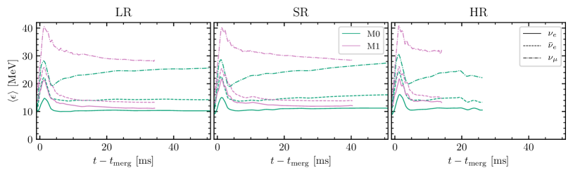
Figure 17: Neutrino average energy comparison between M0 and M1 simulations for all three neutrino species and for the three resolutions in each panel. Neutrinos are extracted at a radius $R_{\mathrm{M0}}=756$ km for the M0 case and $R_{\mathrm{M1}}=443$ km for the M1 case. The data is smoothed using a rolling average with width 1 ms. Time is shifted by the time of merger and by the time of flight of neutrinos to the corresponding detector.

We now discuss the impact of different microphysics and finite resolution effects on the neutrino emission in our simulations. In Fig.16 we show the angle integrated neutrino luminosity for the three neutrino species we simulate, comparing M0 and M1 neutrino schemes for every resolution. Hereafter, we consider one representative heavy flavour neutrino species denoted as $\nu_{\mu}$ with properties calculated as averages over the four neutrino species constituting $\nu_{x}$. Neutrino luminosities for every species present a peak immediately after merger at $\mathcal{L}\approx 10^{52}-10^{53}$ erg s^-1. The hierarchy $\mathcal{L}_{\nu_{\mu}}<\mathcal{L}_{\nu_{e}}<\mathcal{L}_{\bar{\nu}_{e}}$ that we observe in the neutrino luminosity evolution is consistent with previous results (see, e.g., Ruffert et al., 1997; Rosswog et al., 2003; Sekiguchi et al., 2015; Foucart et al., 2016b; Cusinato et al., 2021) and it is explained as follows. Electron antineutrinos are the most abundant species because the positron captures on free neutrons are favoured in the neutron rich ($Y_{e}\approx 0.1$) matter with temperatures of tens of MeV. Electron neutrinos are produced instead mostly due to capture of electrons on protons, which are however not favoured due to the initially low proton abundance. Heavy flavour neutrinos are produced by matter with temperature of tens of MeV emitted from the bouncing remnant. The reactions producing heavy flavour neutrinos are electron-positron annihilation and plasmon decay which are highly dependent on temperature. As the remnant stabilises and cools down, production of heavy flavour neutrinos lowers, while electron/positron captures keep happening in the highest density region of the accretion discs producing electron neutrinos and antineutrinos.

Comparing M0 and M1 runs, we observe that the same luminosity hierarchy is maintained, but M1 scheme predicts larger neutrino brightnesses. The largest difference is observed for heavy flavour neutrinos, where neutrinos in M1 runs are ${\sim}50\%$ brighter than neutrinos in M0 runs.

This is in contrast with Radice et al. (2022), where neutrino luminosities for all species were found a factor ${\sim}3$ larger for M0 compared to M1 scheme. The reason for this difference is that here the neutrino luminosities are computed integrating the proper radiation flux calculated as $\mathcal{F}^{i}=\sqrt{\gamma}(\alpha F^{i}-\beta^{i}E)$ over the sphere, where $E$ and $F^{i}$ are the radiation energy density and the radiation flux in the Eulerian frame, respectively. By contrast, in Radice et al. (2022) neutrino luminosities were computed from the covariant expression $\mathcal{F}_{i}=\sqrt{\gamma}F_{i}$, which is an approximation valid for large extraction radii. Phisically, both quantities are expected to have the same asymptotic value ${\sim}E$, but we find that at our finite radius they differ by a factor ${\sim}3$.

When a BH forms, the emission of heavy flavour neutrinos abruptly stops because this component is emitted from the remnant NS. As resolution increases, we observe an increase in the luminosities at early times, within 15 ms post merger. This is largely explained by the fact that thinner discs are formed at this resolution, which allow neutrinos to diffuse more easily and with shorter timescales. Larger electron antineutrino luminosities at HR, for both M0 and M1 schemes, are in agreement with the fact that larger electron fractions are found in the ejecta distributions for HR.

In Fig.17 we report the neutrino average energies for the same runs. For both M0 and M1 schemes, the energies peak at $2-3$ ms post-merger before reaching a quasi-steady evolution at later times, and follow a hierarchy $\langle\epsilon_{\nu_{e}}\rangle<\langle\epsilon_{\bar{\nu}_{e}}\rangle<\langle\epsilon_{\nu_{\mu}}\rangle$. Focusing on M1 runs, neutrino average energies for heavy lepton neutrinos peak at $40$ MeV and then it decreases below ${\sim}30$ MeV within few tens of ms. Electron antineutrinos and neutrinos follow a similar behaviour also with similar timescales, reaching their maxima at ${\sim}25$ MeV and ${\sim}20$ MeV, and decreasing to ${\sim}12$ MeV and ${\sim}10$ MeV, respectively. Runs with M0 scheme systematically underestimate the energies in the first $t-t_{\mathrm{merg}}=20$ ms by $\approx 30\%$ with respect to M1 runs. We also note that the average energy of the heavy lepton neutrinos increases with time, reaching values comparable to the ones simulated with M1 scheme, within tens of ms post-merger.

The quantitative differences in the $\nu_{e}$ and $\bar{\nu}_{e}$ energies between the two sets of runs possibly originate from different causes. M1 simulations tend to produce more massive and inflated discs. Such discs have more extended neutrino surfaces characterised by lower decoupling temperatures. At the same time, the THC_M1 scheme properly models the diffusion of neutrinos inside the remnant up to the emission at the neutrino surface and their thermalization (Radice et al., 2022). In M0 schemes, instead, the diffusion rate is estimated based on local properties and thermalization effects of diffusing neutrinos are not taken into account. For heavy flavour neutrinos the situation is opposite: neutrinos decouple from matter deep inside the remnant, further diffusing through quasi-isothermal scattering inside the disc. While an M1 scheme is able to catch this effect, retaining larger $\nu_{\mu}$ mean energies, the M0 computes the luminosities and mean energies considering neutrinos in equilibrium with matter everywhere inside the last scattering surface, providing at the same time lower mean energies and larger luminosities. With time, the disc becomes more compact and the diffusion atmosphere reduces in size, so that $\nu_{\mu}$ mean energies become comparable.

The average neutrino energies are not largely influenced by resolution effects. This is expected because the neutrinospheres are mostly determined by the density profile inside the disc (Endrizzi et al., 2020), which we showed to be robust with resolution.

Finally, it is interesting to notice that the value of the high electron fraction peak in the $Y_{e}$ distribution in the ejecta extracted from the M1 runs (and observed at high latitudes) is close to the equilibrium electron fraction, $Y_{e,{\rm eq}}$. The latter can be estimated using eq. 77 of Qian & Woosley (1996). Assuming, according to our neutrino luminosities and mean energies around 10 ms post-merger, $\mathcal{L}_{\bar{\nu}_{e}}\approx 3/2~{}\mathcal{L}_{\nu_{e}}$, $\langle\epsilon_{\nu_{e}}\rangle\approx 12~{}{\rm MeV}$ and $\langle\epsilon_{\bar{\nu}_{e}}\rangle\approx 14~{}{\rm MeV}$, we find $Y_{e,{\rm eq}}\approx 0.46$. This means that in the region above the massive NS absorption rates in the M1 runs are high enough to approach weak equilibrium, and the differences with the M0 results are mostly due to the rates values, rather than to differences in the relative luminosities or mean energies.

8 Conclusions

In this work we performed the first systematic study of the impact of different treatments of neutrino transport on the computation of multi-messenger observables from a BNS merger. Our work is based on ab-initio 3+1 NR simulations performed at three resolutions for each microphysics prescription and up to resolutions of ${\sim}123$ meters (HR) in the strong-field region. We simulated and compared pure hydrodynamics (HY), leakage (LK), leakage+M0 (M0) and M1 neutrino transport schemes. The M0 series of simulations was also repeated with the GRLES subgrid scheme for MHD turbulent viscosity. The simulations considered a BNS merger forming a short-lived remnant; they cover the GW-dominated post-merger phase and last at least ${\sim}15$ ms and up to 140 ms post-merger.

Our analysis indicates that the gravitational collapse of the short lived remnant is mainly determined by the emission of GWs and angular momentum transport. Turbulent viscosity can significantly affect the collapse by stabilizing the remnant, whereas the impact of different neutrino schemes is negligible. BH collapse happens as the remnant approaches the maximum density of the corresponding cold, $\beta$-equilibrated spherically symmetric equilibria (Perego et al., 2022), in particular for $\rho_{\mathrm{max}}\gtrsim 70\%\rho_{\mathrm{max}}^{\mathrm{TOV}}$. The remnant’s stability and the time of collapse are strongly affected by the grid resolutions. In our setup, high resolutions generically induce an earlier collapse while numerical effects at low resolutions can stabilise the remnant. Nonetheless, we find that the remnant’s bulk dynamics can be robustly studied using the gauge-invariant curves of binding energy and maximum rest-mass density. As shown in Fig. 2, these quantities are strongly correlated and the correlation is not sensitively dependent on the grid resolution. This implies the possibility of probing the maximum remnant densities from inferences of the emitted GW energy (Radice et al., 2017).

Accretion discs of initial masses up to $M_{b}^{\mathrm{disc}}\approx 0.2~{}{\rm M_{\odot}}$ form around the remnant NS during merger. The disc masses depend on the microphysics prescription used: LK simulations produce the least massive disc, while HY simulations produce the most massive disc (for sufficiently high resolutions). In general, including neutrino transport leads to more inflated discs with respect to pure hydro. The electron fraction of disc matter at low latitudes reaches values of $\approx 0.25$ for LK schemes, but is larger in M0 and VM0 runs comparing matter shells at same density. At lower densities or higher latitudes, M0 schemes predicts $Y_{e}\gtrsim 0.3$. The M1 scheme leads to the largest $Y_{e}\gtrsim 0.42$. Increasing the grid resolution leads to the formation of less massive, more compact discs but it does not significantly affect their composition. However, the disc mass and accretion rates are heavily dependent on black formation, which in turn is affected by resolution (see above). Overall, our analysis indicates that advanced transport scheme are absolutely necessary in future long-term disc evolutions, and LK schemes should be abandoned. At the same time, post-merger simulations at mesh resolutions above 200 meters seem insufficient to deliver quantitative results for astrophysical predictions.

Simulations with M1 transport show the emergence of a neutrino trapped gas in the remnant’s NS core (Foucart et al., 2016b; Perego et al., 2019; Radice et al., 2022). The neutrino gas locally decreases the temperature and increases $Y_{e}$ by ${\sim}30~{}\%$ comparing to LK runs. We do not observe changes in the pressure and consequent alterations in the gravitational collapse in our models. The abundances of the neutrino species in the trapped gas are in the hierarchy $Y_{\nu_{e}}<Y_{\nu_{x}}<Y_{\bar{\nu}_{e}}$, that can be understood from the thermodynamics conditions in the remnant NS core (Perego et al., 2019).

GW emission is not significantly affected by microphysics in the considered BNS, despite the latter being a binary that produces a short-lived remnant close to the collapse. The main GW properties can be robustly extracted from simulations with at least SR resolution. Our post-merger faithfulness analysis indicates that, at SR and HR resolutions, the waveform quality is sufficient for an accurate modeling of post-merger signals. This precision is sufficient for both detecting post-merger signals with matched-filter analyses and for constraining the EOS at extreme matter densities with third generation observations (Breschi et al., 2022). In contrast to Refs. Most et al. (2022); Hammond et al. (2022), our high-resolution M1 simulations do not show any evidence of a significant out-of-equilibrium and bulk viscosity effects in the GWs. The key differences between our work and previous ones is the consistent treatment of neutrino radiation and the higher grid resolution (more than a factor 3 higher in our HR runs).

In our simulations, ejecta of $M_{\mathrm{ej}}\gtrsim 2\times 10^{-3}$ are launched during merger, with the smallest (largest) ejection measured in LK (HY) runs. Increasing the resolution typically decreases the ejecta mass. The largest deviation is $\approx 50\%$ (VM0-SR and VM0-HR), that could be taken as an estimate of the current NR uncertainties. We find that the early ejecta mass as a function of the ejecta velocity can be modelled with a two-components broken power-law of type $\propto(\beta\gamma/\left(\beta\gamma\right)_{\beta_{0}})^{-s}$, with $\beta_{0}\in[0.3,\,0.45]$. The most massive and slower component has $s_{\mathrm{KN}}\approx 0.64-1.6$ for $v<\beta_{0}c$, whereas the fast tail component has a steeper profile, $s_{\mathrm{ft}}\gtrsim 4-11$, and masses $M_{\mathrm{ej}}(v_{\infty}>\beta_{0}c)\approx 10^{-5}-10^{-4}~{}{\rm M_{\odot}}$. The $Y_{e}$ distribution in the dynamical ejecta largely depends on the simulated microphysics. In all LR and SR runs we observe very neutron rich ejecta component at low latitudes, corresponding to the tidal component. The LK scheme predicts a second peak in the $Y_{e}$ distribution at $Y_{e}\approx 0.13-0.17$, corresponding to the shock-heated component. Matter leptonization due to neutrinos emitted by the remnant and reabsorbed in the ejecta produces a broader peak in the $Y_{e}$ distribution of the runs with M0, spanning $Y_{e}\approx 0.2-0.35$. M1 simulations show an additional high-$Y_{e}$ peak at $Y_{e}\approx 0.425$, corresponding to material emitted at high latitudes. With the only exception of VM0-HR, we note that the low-$Y_{e}$ peak is suppressed in HR runs due to two reasons. First, the tidal component is smaller because the remnant star is more compact than in lower resolution runs. Second, discs at HR are thinner and less massive than lower resolutions ones, thus less opaque to neutrinos. This effect is mitigated in VM0-HR run, where viscosity effects produce a larger disc compared to the other HR runs.

Our results confirm the relevant role of neutrinos emission and absorption in shaping the nucleosynthesis yields from the early time ejecta. Both M0 or M1 schemes deliver, at high-resolutions, comparable abundances and reproduce well the observed solar residual pattern. On the contrary, the LK scheme alone underestimates the abundances of light $r$-process elements, since neutrino reabsorption is required to produce the ejecta conditions suitable for the production of those elements.

The calculated kilonova light curves are rather robust against grid resolution but are very sensitive to the cumulative time during which ejecta are measured and to the effect of neutrino irradiation. Larger ejecta masses and lower $Y_{e}$ generate brigther kilonova light curves. Accordingly, HY (LK) runs produce the brightest (dimmest) kilonovae as shown in Fig. 15. However, the largest light curve variations in the plot are associated to the use of the ejecta calculated over different time intervals. During these times the ejecta mass increases and the ejecta composition changes due to an early wind component summing up to the dynamical ejecta. These results highlight, once again, the critical need for long-term merger and post-merger simulations with realistic microphysics for the reliable prediction of the EM counterparts to mergers.

We find neutrino luminosities of the order of $\mathcal{L}\approx 10^{52}-10^{53}$. M0 runs slightly underestimate the neutrino luminosity with respect to M1 runs, for each simulated neutrino species. This difference is largest in the case of heavy flavour neutrinos, because only M1 schemes are able to simulate their diffusion inside the disc. However, in both cases the two schemes consistently predict the hierarchy $\mathcal{L}_{\nu_{\mu}}<\mathcal{L}_{\nu_{e}}<\mathcal{L}_{\bar{\nu}_{e}}$. These results confirm previous findings (Foucart et al., 2016b; Radice et al., 2022) and stresses the importance of using M1 schemes for detailed predictions. Larger $\mathcal{L}_{\bar{\nu}_{e}}$ are found at HR, which is explained by the presence of thinner discs. This is consistent with the ejecta composition summarised above and in particular it is related to the suppression of the low-$Y_{e}$ peak in HR $Y_{e}$ distribution.

Our work highlights the fact that both resolution and microphysics can have a significant impact on the observables predicted by a BNS merger simulation. Future work will be focused on extending M1 simulations to different binaries and for longer times after merger. Our results indicate that advanced neutrino schemes, like the M1, and sub-grid-MHD effects are likely necessary physics input for an accurate prediction of the winds from the remnant. At the same time, high-resolution simulations appear essential for robust results in long-term evolutions.

Data Availability

Data generated for this study will be made available upon reasonable request to the corresponding authors.

References

- Abbott et al. (2017a) Abbott B. P., et al., 2017a, Astrophys. J., 848, L12
- Abbott et al. (2017b) Abbott B. P., et al., 2017b, Astrophys. J., 848, L13
- Abbott et al. (2017c) Abbott B. P., et al., 2017c, Astrophys. J., 850, L39
- Abbott et al. (2019a) Abbott R., et al., 2019a
- Abbott et al. (2019b) Abbott B. P., et al., 2019b, Phys. Rev., X9, 011001
- Aguilera-Miret et al. (2020) Aguilera-Miret R., Viganò D., Carrasco F., Miñano B., Palenzuela C., 2020, Phys. Rev. D, 102, 103006
- Alford et al. (2018) Alford M. G., Bovard L., Hanauske M., Rezzolla L., Schwenzer K., 2018, Phys. Rev. Lett., 120, 041101
- Arcavi et al. (2017) Arcavi I., et al., 2017, Nature, 551, 64
- Ardevol-Pulpillo et al. (2019) Ardevol-Pulpillo R., Janka H. T., Just O., Bauswein A., 2019, Mon. Not. Roy. Astron. Soc., 485, 4754
- Arlandini et al. (1999) Arlandini C., Kaeppeler F., Wisshak K., Gallino R., Lugaro M., Busso M., Straniero O., 1999, Astrophys. J., 525, 886
- Berger & Colella (1989) Berger M. J., Colella P., 1989, Journal of Computational Physics, 82, 64
- Berger & Oliger (1984) Berger M. J., Oliger J., 1984, J.Comput.Phys., 53, 484
- Bernuzzi (2020) Bernuzzi S., 2020, Gen. Rel. Grav., 52, 108
- Bernuzzi & Hilditch (2010) Bernuzzi S., Hilditch D., 2010, Phys. Rev., D81, 084003
- Bernuzzi et al. (2012a) Bernuzzi S., Thierfelder M., Brügmann B., 2012a, Phys.Rev., D85, 104030
- Bernuzzi et al. (2012b) Bernuzzi S., Nagar A., Thierfelder M., Brügmann B., 2012b, Phys.Rev., D86, 044030
- Bernuzzi et al. (2016) Bernuzzi S., Radice D., Ott C. D., Roberts L. F., Mösta P., Galeazzi F., 2016, How loud are neutron star mergers?, doi:10.5281/zenodo.57844, https://doi.org/10.5281/zenodo.57844
- Bernuzzi et al. (2020) Bernuzzi S., et al., 2020, Mon. Not. Roy. Astron. Soc.
- Breschi et al. (2019) Breschi M., Bernuzzi S., Zappa F., Agathos M., Perego A., Radice D., Nagar A., 2019, Phys. Rev., D100, 104029
- Breschi et al. (2021) Breschi M., Perego A., Bernuzzi S., Del Pozzo W., Nedora V., Radice D., Vescovi D., 2021, Mon. Not. Roy. Astron. Soc., 505, 1661
- Breschi et al. (2022) Breschi M., Bernuzzi S., Chakravarti K., Camilletti A., Prakash A., Perego A., 2022
- Bruenn (1985) Bruenn S. W., 1985, Astrophys. J. Suppl., 58, 771
- Burrows et al. (2006) Burrows A., Reddy S., Thompson T. A., 2006, Nucl. Phys., A777, 356
- Camilletti et al. (2022) Camilletti A., et al., 2022, ] 10.1093/mnras/stac2333
- Chatziioannou et al. (2017) Chatziioannou K., Klein A., Yunes N., Cornish N., 2017, Phys. Rev., D95, 104004
- Chornock et al. (2017) Chornock R., et al., 2017, Astrophys. J., 848, L19
- Ciolfi (2020) Ciolfi R., 2020, Mon. Not. Roy. Astron. Soc., 495, L66
- Ciolfi et al. (2019) Ciolfi R., Kastaun W., Kalinani J. V., Giacomazzo B., 2019, Phys. Rev., D100, 023005
- Combi & Siegel (2022) Combi L., Siegel D., 2022
- Coulter et al. (2017) Coulter D. A., et al., 2017, Science
- Cowan et al. (2021) Cowan J. J., Sneden C., Lawler J. E., Aprahamian A., Wiescher M., Langanke K., Martínez-Pinedo G., Thielemann F.-K., 2021, Rev. Mod. Phys., 93, 15002
- Cowperthwaite et al. (2017) Cowperthwaite P. S., et al., 2017, Astrophys. J., 848, L17
- Cromartie et al. (2019) Cromartie H. T., et al., 2019, Nat. Astron., 4, 72
- Cusinato et al. (2021) Cusinato M., Guercilena F. M., Perego A., Logoteta D., Radice D., Bernuzzi S., Ansoldi S., 2021, ] 10.1140/epja/s10050-022-00743-5
- Cutler & Flanagan (1994) Cutler C., Flanagan E. E., 1994, Phys.Rev., D49, 2658
- Damour et al. (2011) Damour T., Nagar A., Trias M., 2011, Phys. Rev., D83, 024006
- Damour et al. (2012) Damour T., Nagar A., Pollney D., Reisswig C., 2012, Phys.Rev.Lett., 108, 131101
- Dessart et al. (2009) Dessart L., Ott C., Burrows A., Rosswog S., Livne E., 2009, Astrophys.J., 690, 1681
- Douchin & Haensel (2001) Douchin F., Haensel P., 2001, Astron. Astrophys., 380, 151
- Drout et al. (2017) Drout M. R., et al., 2017, Science, 358, 1570
- Duez et al. (2004) Duez M. D., Liu Y. T., Shapiro S. L., Stephens B. C., 2004, Phys.Rev., D69, 104030
- Duez et al. (2008) Duez M. D., Foucart F., Kidder L. E., Pfeiffer H. P., Scheel M. A., Teukolsky S. A., 2008, Phys. Rev., D78, 104015
- Eichler et al. (1989) Eichler D., Livio M., Piran T., Schramm D. N., 1989, Nature, 340, 126
- (44) http://www.einsteintoolkit.org
- Endrizzi et al. (2020) Endrizzi A., et al., 2020, Eur. Phys. J. A, 56, 15
- Evans et al. (2017) Evans P. A., et al., 2017, Science, 358, 1565
- Fernández et al. (2015) Fernández R., Quataert E., Schwab J., Kasen D., Rosswog S., 2015, Mon. Not. Roy. Astron. Soc., 449, 390
- Fernández et al. (2019) Fernández R., Tchekhovskoy A., Quataert E., Foucart F., Kasen D., 2019, Mon. Not. Roy. Astron. Soc., 482, 3373
- Fonseca et al. (2021) Fonseca E., et al., 2021, Astrophys. J. Lett., 915, L12
- Foucart et al. (2015) Foucart F., et al., 2015, Phys. Rev., D91, 124021
- Foucart et al. (2016a) Foucart F., et al., 2016a, Phys. Rev., D93, 044019
- Foucart et al. (2016b) Foucart F., O’Connor E., Roberts L., Kidder L. E., Pfeiffer H. P., Scheel M. A., 2016b, Phys. Rev., D94, 123016
- Foucart et al. (2020) Foucart F., Duez M. D., Hebert F., Kidder L. E., Pfeiffer H. P., Scheel M. A., 2020, Astrophys. J. Lett., 902, L27
- Foucart et al. (2021) Foucart F., Moesta P., Ramirez T., Wright A. J., Darbha S., Kasen D., 2021
- Fujibayashi et al. (2017) Fujibayashi S., Sekiguchi Y., Kiuchi K., Shibata M., 2017, Astrophys. J., 846, 114
- Fujibayashi et al. (2018) Fujibayashi S., Kiuchi K., Nishimura N., Sekiguchi Y., Shibata M., 2018, Astrophys. J., 860, 64
- Fujibayashi et al. (2020) Fujibayashi S., Shibata M., Wanajo S., Kiuchi K., Kyutoku K., Sekiguchi Y., 2020, Phys. Rev. D, 101, 083029
- Galeazzi et al. (2013) Galeazzi F., Kastaun W., Rezzolla L., Font J. A., 2013, Phys.Rev., D88, 064009
- Ghirlanda et al. (2019) Ghirlanda G., et al., 2019, Science, 363, 968
- Gizzi et al. (2021) Gizzi D., Lundman C., O’Connor E., Rosswog S., Perego A., 2021, Mon. Not. Roy. Astron. Soc., 505, 2575
- Goodale et al. (2003) Goodale T., Allen G., Lanfermann G., Massó J., Radke T., Seidel E., Shalf J., 2003, in Vector and Parallel Processing – VECPAR’2002, 5th International Conference, Lecture Notes in Computer Science. Springer, Berlin
- Goriely et al. (2015) Goriely S., Bauswein A., Just O., Pllumbi E., Janka H.-T., 2015, Mon. Not. Roy. Astron. Soc., 452, 3894
- Gottlieb & Ketcheson (2009) Gottlieb S., Ketcheson David I.and Shu C.-W., 2009, Journal of Scientific Computing, 38, 251
- Gourgoulhon et al. (2016) Gourgoulhon E., Grandclément P., Marck J.-A., Novak J., Taniguchi K., 2016
- Hajela et al. (2022) Hajela A., et al., 2022, Astrophys. J. Lett., 927, L17
- Hallinan et al. (2017) Hallinan G., et al., 2017, Science, 358, 1579
- Hammond et al. (2022) Hammond P., Hawke I., Andersson N., 2022
- Hanauske et al. (2017) Hanauske M., Takami K., Bovard L., Rezzolla L., Font J. A., Galeazzi F., Stöcker H., 2017, Phys. Rev. D, 96, 043004
- Hilditch et al. (2013) Hilditch D., Bernuzzi S., Thierfelder M., Cao Z., Tichy W., Bruegmann B., 2013, Phys. Rev., D88, 084057
- Hotokezaka et al. (2013) Hotokezaka K., Kiuchi K., Kyutoku K., Muranushi T., Sekiguchi Y.-i., et al., 2013, Phys.Rev., D88, 044026
- Hotokezaka et al. (2018) Hotokezaka K., Kiuchi K., Shibata M., Nakar E., Piran T., 2018, Astrophys. J., 867, 95
- Janiuk (2019) Janiuk A., 2019, ] 10.3847/1538-4357/ab3349
- Just et al. (2015) Just O., Bauswein A., Pulpillo R. A., Goriely S., Janka H. T., 2015, Mon. Not. Roy. Astron. Soc., 448, 541
- Just et al. (2016) Just O., Obergaulinger M., Janka H. T., Bauswein A., Schwarz N., 2016, Astrophys. J. Lett., 816, L30
- Just et al. (2021) Just O., Goriely S., Janka H.-T., Nagataki S., Bauswein A., 2021, Mon. Not. Roy. Astron. Soc., 509, 1377
- Kasliwal et al. (2017) Kasliwal M. M., et al., 2017, Science, 358, 1559
- Kastaun et al. (2016) Kastaun W., Ciolfi R., Giacomazzo B., 2016, Phys. Rev. D, 94, 044060
- Kawaguchi et al. (2018) Kawaguchi K., Shibata M., Tanaka M., 2018, Astrophys. J., 865, L21
- Kawaguchi et al. (2020) Kawaguchi K., Shibata M., Tanaka M., 2020, Astrophys. J., 889, 171
- Kiuchi et al. (2014) Kiuchi K., Kyutoku K., Sekiguchi Y., Shibata M., Wada T., 2014, Phys.Rev., D90, 041502
- Kiuchi et al. (2015) Kiuchi K., Cerdá-Durán P., Kyutoku K., Sekiguchi Y., Shibata M., 2015, Phys. Rev. D, 92, 124034
- Kiuchi et al. (2018) Kiuchi K., Kyutoku K., Sekiguchi Y., Shibata M., 2018, Phys. Rev., D97, 124039
- Korobkin et al. (2020) Korobkin O., et al., 2020
- LIGO Scientific Collaboration (2018) LIGO Scientific Collaboration 2018, LIGO Algorithm Library - LALSuite, free software (GPL), doi:10.7935/GT1W-FZ16
- Lippuner et al. (2017) Lippuner J., Fernández R., Roberts L. F., Foucart F., Kasen D., Metzger B. D., Ott C. D., 2017, Mon. Not. Roy. Astron. Soc., 472, 904
- Loffler et al. (2012) Loffler F., et al., 2012, Class. Quant. Grav., 29, 115001
- Loffredo et al. (2022) Loffredo E., Perego A., Logoteta D., Branchesi M., 2022
- Lyman et al. (2018) Lyman J. D., et al., 2018, Nat. Astron., 2, 751
- Martin et al. (2015) Martin D., Perego A., Arcones A., Thielemann F.-K., Korobkin O., Rosswog S., 2015, Astrophys. J., 813, 2
- Martin et al. (2018) Martin D., Perego A., Kastaun W., Arcones A., 2018, Class. Quant. Grav., 35, 034001
- Metzger & Fernández (2014) Metzger B. D., Fernández R., 2014, Mon.Not.Roy.Astron.Soc., 441, 3444
- Metzger et al. (2018) Metzger B. D., Thompson T. A., Quataert E., 2018, Astrophys. J., 856, 101
- Miller et al. (2019a) Miller M. C., et al., 2019a, Astrophys. J., 887, L24
- Miller et al. (2019b) Miller J. M., et al., 2019b, Phys. Rev., D100, 023008
- Mooley et al. (2018) Mooley K. P., et al., 2018, Nature, 561, 355
- Morozova et al. (2015) Morozova V., Piro A. L., Renzo M., Ott C. D., Clausen D., Couch S. M., Ellis J., Roberts L. F., 2015, Astrophys. J., 814, 63
- Most et al. (2022) Most E. R., Haber A., Harris S. P., Zhang Z., Alford M. G., Noronha J., 2022
- Mösta et al. (2020) Mösta P., Radice D., Haas R., Schnetter E., Bernuzzi S., 2020, Astrophys. J. Lett., 901, L37
- Mumpower et al. (2017) Mumpower M. R., McLaughlin G. C., Surman R., Steiner A. W., 2017, J. Phys. G, 44, 034003
- Nakar & Piran (2018) Nakar E., Piran T., 2018, Mon. Not. Roy. Astron. Soc., 478, 407
- Nedora et al. (2019) Nedora V., Bernuzzi S., Radice D., Perego A., Endrizzi A., Ortiz N., 2019, Astrophys. J., 886, L30
- Nedora et al. (2021a) Nedora V., Radice D., Bernuzzi S., Perego A., Daszuta B., Endrizzi A., Prakash A., Schianchi F., 2021a, preprint (ArXiv:2104.04537)
- Nedora et al. (2021b) Nedora V., et al., 2021b, Astrophys. J., 906, 98
- Nedora et al. (2022) Nedora V., et al., 2022, Class. Quant. Grav., 39, 015008
- Neilsen et al. (2014) Neilsen D., Liebling S. L., Anderson M., Lehner L., O’Connor E., et al., 2014, Phys.Rev., D89, 104029
- Nicholl et al. (2017) Nicholl M., et al., 2017, Astrophys. J., 848, L18
- Palenzuela et al. (2015) Palenzuela C., Liebling S. L., Neilsen D., Lehner L., Caballero O. L., O’Connor E., Anderson M., 2015, Phys. Rev., D92, 044045
- Perego et al. (2014) Perego A., Rosswog S., Cabezon R., Korobkin O., Kaeppeli R., et al., 2014, Mon.Not.Roy.Astron.Soc., 443, 3134
- Perego et al. (2017a) Perego A., Radice D., Bernuzzi S., 2017a, Astrophys. J., 850, L37
- Perego et al. (2017b) Perego A., Yasin H., Arcones A., 2017b, J. Phys., G44, 084007
- Perego et al. (2019) Perego A., Bernuzzi S., Radice D., 2019, Eur. Phys. J., A55, 124
- Perego et al. (2021) Perego A., Thielemann F. K., Cescutti G., 2021, in , Handbook of Gravitational Wave Astronomy. p. 1, doi:10.1007/978-981-15-4702-7_13-1
- Perego et al. (2022) Perego A., Logoteta D., Radice D., Bernuzzi S., Kashyap R., Das A., Padamata S., Prakash A., 2022, Phys. Rev. Lett., 129, 032701
- Qian & Woosley (1996) Qian Y., Woosley S., 1996, Astrophys. J., 471, 331
- Radice (2017) Radice D., 2017, Astrophys. J., 838, L2
- Radice (2020) Radice D., 2020, Symmetry, 12, 1249
- Radice & Rezzolla (2012) Radice D., Rezzolla L., 2012, Astron. Astrophys., 547, A26
- Radice et al. (2014a) Radice D., Rezzolla L., Galeazzi F., 2014a, Class.Quant.Grav., 31, 075012
- Radice et al. (2014b) Radice D., Rezzolla L., Galeazzi F., 2014b, Mon.Not.Roy.Astron.Soc., 437, L46
- Radice et al. (2015) Radice D., Rezzolla L., Galeazzi F., 2015, ASP Conf. Ser., 498, 121
- Radice et al. (2016) Radice D., Galeazzi F., Lippuner J., Roberts L. F., Ott C. D., Rezzolla L., 2016, Mon. Not. Roy. Astron. Soc., 460, 3255
- Radice et al. (2017) Radice D., Bernuzzi S., Del Pozzo W., Roberts L. F., Ott C. D., 2017, Astrophys. J., 842, L10
- Radice et al. (2018a) Radice D., Perego A., Bernuzzi S., Zhang B., 2018a, Mon. Not. Roy. Astron. Soc., 481, 3670
- Radice et al. (2018b) Radice D., Perego A., Hotokezaka K., Fromm S. A., Bernuzzi S., Roberts L. F., 2018b, Astrophys. J., 869, 130
- Radice et al. (2020) Radice D., Bernuzzi S., Perego A., 2020, Ann. Rev. Nucl. Part. Sci., 70
- Radice et al. (2022) Radice D., Bernuzzi S., Perego A., Haas R., 2022, Mon. Not. Roy. Astron. Soc., 512, 1499
- Reisswig & Pollney (2011) Reisswig C., Pollney D., 2011, Class.Quant.Grav., 28, 195015
- Reisswig et al. (2013a) Reisswig C., Ott C., Abdikamalov E., Haas R., Mösta P., et al., 2013a, Phys.Rev.Lett., 111, 151101
- Reisswig et al. (2013b) Reisswig C., Haas R., Ott C. D., Abdikamalov E., Mösta P., Pollney D., Schnetter E., 2013b, Phys. Rev., D87, 064023
- Riley et al. (2019) Riley T. E., et al., 2019, Astrophys. J., 887, L21
- Rosswog & Korobkin (2022) Rosswog S., Korobkin O., 2022
- Rosswog & Liebendoerfer (2003) Rosswog S., Liebendoerfer M., 2003, Mon.Not.Roy.Astron.Soc., 342, 673
- Rosswog & Ramirez-Ruiz (2002) Rosswog S., Ramirez-Ruiz E., 2002, Mon.Not.Roy.Astron.Soc., 336, L7
- Rosswog et al. (2003) Rosswog S., Ramirez-Ruiz E., Davies M. B., 2003, Mon. Not. Roy. Astron. Soc., 345, 1077
- Ruan et al. (2018) Ruan J. J., Nynka M., Haggard D., Kalogera V., Evans P., 2018, Astrophys. J., 853, L4
- Ruffert et al. (1997) Ruffert M., Janka H., Takahashi K., Schäfer G., 1997, Astron.Astrophys., 319, 122
- Schneider et al. (2017) Schneider A. S., Roberts L. F., Ott C. D., 2017, Phys. Rev., C96, 065802
- Schnetter et al. (2004) Schnetter E., Hawley S. H., Hawke I., 2004, Class.Quant.Grav., 21, 1465
- Schnetter et al. (2007) Schnetter E., Ott C. D., Allen G., Diener P., Goodale T., Radke T., Seidel E., Shalf J., 2007
- Sekiguchi (2010) Sekiguchi Y., 2010, Prog. Theor. Phys., 124, 331
- Sekiguchi et al. (2011) Sekiguchi Y., Kiuchi K., Kyutoku K., Shibata M., 2011, Phys.Rev.Lett., 107, 051102
- Sekiguchi et al. (2015) Sekiguchi Y., Kiuchi K., Kyutoku K., Shibata M., 2015, Phys.Rev., D91, 064059