On the economic viability of solar energy when upgrading cellular networks

Abstract

The massive increase of data traffic, the widespread proliferation of wireless applications and the full-scale deployment of 5G and the IoT, imply a steep increase in cellular networks energy use, resulting in a significant carbon footprint. This paper presents a comprehensive model to show the interaction between the networking and energy features of the problem and study the economical and technical viability of green networking. Solar equipment, cell zooming, energy management and dynamic user allocation are considered in the upgrading network planning process. We propose a mixed-integer optimization model to minimize long-term capital costs and operational energy expenditures in a heterogeneous on-grid cellular network with different types of base station, including solar. Based on eight scenarios where realistic costs of solar panels, batteries, and inverters were considered, we first found that solar base stations are currently not economically interesting for cellular operators. We next studied the impact of a significant and progressive carbon tax on reducing greenhouse gas emissions (GHG). We found that, at current energy and equipment prices, a carbon tax ten-fold the current value is the only element that could make green base stations economically viable.

I Introduction

Cellular operators are facing traffic growth due to the increasing use of mobile applications [1] and the rapid development of wireless access technologies such as 5G and beyond. To meet this demand, new base stations (BSs) are being added or upgraded to the next generation technologies [2].

We claim that this current and future upgrading of cellular systems provides a great opportunity for operators to reduce their environmental impact. The COP21 Paris agreement has set a target limit of 2°C for the global warming. In that context, the Information and Communication Technologies sector has a role to play given that it accounts for about 4% of the global energy use [3] and has generated approximately between 1.8% to 2.8% of the global GHG emissions in 2020 [4]. A significant part of this is produced by cellular networks [5] which generate the equivalent of 220 MtCO2, which represents 0.4% of global emissions [6]. It is estimated [7] that the full deployment of 5G could have an environmental impact up to 2 to 3 times larger. Moving to the millimeter wavebands [1] will reduce the range of the new 5G antennas. This in turn will require a much more dense radio infrastructure [8] with the ensuing large increase in energy use.

One solution is to wait for the grid to use energy sources that don’t emit CO2. This is a major undertaking that will take years to be implemented. In this paper, we look at a different approach to reduce the emissions of the wireless networks. We posit that it is possible to reduce both OPEX and CO2 emissions by carefully integrating the energy management features within the planning process while taking into account the CAPEX cost.

The idea is to make use of technology that is either currently available or that will become more common with 5G full deployment: sleep mode, cell zooming, user allocation and solar power. These can be implemented gradually as the need arises and do not depend on the general greening of the power grid. More specifically, we want to see if this evolution can be driven by market economics where the savings provided by the reduction in grid costs are sufficient to cover the additional capital cost of the equipment. In cases where this is not possible, we want to see to what extent a carbon tax can drive the process.

For this, we propose a model to evaluate the combined technical and economic viability of future green cellular networks. This is done by a detailed modeling of energy, communication and demand features and by an in-depth study on how the issues of energy management, solar energy, CO2 emission, CAPEX and OPEX are interrelated.

II Literature Review

The literature relevant to this work is very large, encompassing the use of solar equipment, energy management, dynamic user assignment and green planning. In what follows, we go through a quick technological and literature survey of each one of those areas.

II-A Solar Equipment

Solar panels have been obvious candidates for green networks for more than 10 years (See references in [9]). The main advantage of solar energy is the fact that the cost per kW has been decreasing steadily over the last 10 years and is currently the lowest of the more frequently used green sources [10]. Solar panels are particularly useful and coveted for power stations in remote areas not covered by the power grid and that use non-renewable resources. An extreme case is off-grid rural areas where base stations are just diesel powered.

For instance, the technique proposed in [11] decreases both OPEX and greenhouse gas emissions for remote rural base stations in Malaysia using solar photovoltaic/diesel generator hybrid power systems. The economical and environmental viability of PV/diesel/battery hybrid system configuration for a BS in Nigeria was examined in [12]. Due to the large amount of solar energy available, this system offers an alternative power source for a BS by reducing operational costs and emissions of greenhouse gases. A solar PV/Fuel cell hybrid system under the software HOMER is proposed in [13] to power a remote base station in Ghana. The objective is to reduce both greenhouse gas emissions and lower the levelized cost of electricity (LCOE). In this hybrid system, the LCOE is reduced by 67% compared to diesel power. Similarly, the authors of [14] use the HOMER software to simulate PV-battery-diesel to power a BS during 24 hours under South African climate. They minimize operation costs, emissions, and power use. The potential of photovoltaic to power BS is studied in [15] for Kuwait where the HOMER software is used to determine the number of PV, batteries, and converters for an off-grid solar PV system with diesel generator while minimizing the net present cost in order to power a cellular BSs.

There have also been some urban implementations. The work of [16] studies a case in urban areas of South Korea where both on- and off-grid sites use standalone solar batteries to power a macro LTE cellular base station. A multi-objective optimization algorithm is proposed in [17] for the optimal sizing of a standalone PV/battery to power a BS under the climate of Sydney. The objective is the minimum annual total life cost. An optimal decision of demand-side power management for a green wireless base station is proposed in [18] to minimize the power cost and provide flexibility under traffic load, grid power price, and renewable source uncertainties.

These studies, rural or urban, all have something in common: they refer to a single base station and, in most cases, they lack accounting for the replacement, degradation and installation costs for the solar equipment.

II-B Energy Management and Dynamic User Assignment

Given that 80% of the energy used by a cellular network comes from the radio infrastructure [19], radio energy management must become an integral part of the base station operation. Even though the existing management tools are performance-oriented, they make it possible to design management strategies that can also be used to reduce energy use, based on the fact that real-world data shows that most base stations are underutilized during low traffic periods [20].

In fact, it has already been shown that dynamic management may potentially save between 20% to 30% of energy [21] in cellular networks if the system is planned from the start with enough base stations. These savings are obtained either by completely turning off some base stations or by reducing their power during key times of the day. Even though these methods are nothing new, they will be more easily implemented in 5G networks and beyond using the notion of cell zooming.

The actual operation of cell zooming can be viewed in two ways. In [22], the total available power can be reassigned arbitrarily among radio blocks which in turn can be allocated to different down-link transmissions. It is also stated in [23, 24] that a cell can extend its range through zooming. An extreme case of cell zooming is putting some base stations in sleep mode [25, 26, 27, 28], or even turning them off completely whenever user demand is lower. Different objective metrics have been used such as coverage [29], user demand [30] or the actual power usage [31]. A multi-criteria model is presented in [32] to minimize both the energy use and the user drop probability.

A nonlinear model to minimize energy use subject to quality of service constraints is proposed in [33]. The technique described in [34] uses solar power and on-off operation to minimize energy cost by assigning users to different base stations and choosing solar or grid power during the day.

One consequence of sleep mode or cell zooming is that one must re-assign users to different base stations during the day whenever a user can no longer be served by its base station due to a power reduction. This has been examined in detail in [35, 36, 37]. The conclusion was that dynamic user assignment can reduce the network cost significantly when it is integrated into the long-term planning model. These results will not be repeated here in order to conserve space.

II-C Green Planning

The techniques described above can be viewed as network management and operate on a short-term horizon of minutes or hours. Network planning, on the other hand, where one has to decide on the installation of base stations and the equipment to go with it, works on a time scale of many years. This is by itself a complex procedure since one needs to combine cells of different sizes, including macro, micro, pico, and femto cells. The size of base stations depends on several factors, including the site location and the antenna position. Small stations serve areas with high traffic density using a lower amount of energy [38, 39] but need to be combined with larger base stations for lower-density areas.

Because of the large difference in time scales, the process was often split into two independent parts: plan the equipment upgrades every year and manage the resulting network on a shorter scale using the equipment available.

Unfortunately, network planning and network management are tightly coupled because one cannot use a network management technique, such as solar cells, if the equipment has not been installed. In fact, it has been shown that integrating the technology choice with the long-term planning process produces networks significantly cheaper than a two-step procedure [35, 36, 37]. There is thus a definite need for an integrated model that takes into account the effect of short-term management techniques when deciding on equipment upgrades.

The problem of minimizing the total CAPEX and OPEX cost over a 10-year horizon has been examined, albeit for a single base station, in [40]. They make a detailed model of the energy interactions and study the trade-off between solar panels, a diesel generator or grid power. A similar energy approach was presented in [34] when minimizing the energy cost of a given network. The variables are the allocation of users to base stations and the energy source used by each base station during each one of a given number of time intervals. Even though both [40] and [34] study the energy planning of the network, neither treats the networking planning problem, in particular the decision of where and when to locate new green base stations over the planning horizon.

Some limited work has been done on related topics. The allocation of users over a single day to maximize the network operator’s revenue has been examined in [41].

The work of [42] explores the long-term network planning with green energy harvesting of solar or wind sources. The problem is to select a subset of candidate BSs and to assign users to the available base stations subject to a minimum SINR requirement in order to minimize the base station installation and the user connection costs and the cost of electric grid.

The first attempt at integrating the short-term benefits of solar energy and network planning has been presented in our previous work [37]. The goal was to minimize the total operating plus capital cost of the network. The users can be re-assigned and the base station antennas can be switched off depending on the demand at different times of day.

Some work has also considered a marketing-oriented approach. A financial analysis of network upgrade is described in [43] to optimize the trade-off between the generated revenue produced by the upgrade and its cost. A dynamic programming model is proposed and a fast heuristic solution is used to compute solutions. A similar approach is used in [44] where a case study is presented to evaluate the impact of energy trading either between base stations or through an energy broker and also with spectrum sharing between operators.

II-D Our contribution

Differently from the above body of work, this paper proposes a comprehensive approach to study not just the technical or the economic viability of using solar equipment to update cellular networks, but the interaction between the two. The strength of our contribution to the state of the art comes from a detailed model of energy management and networking planning. It is precisely this level of detail what allows us to clarify the technical and economic features of network upgrade.

1. We integrate the short-term network and energy management with the long-term network expansion over many years into a single model to provide a more realistic view of how the planning and operation are inter-related.

2. The planning determines decisions on different base stations sizes and types, including solar panels, that are needed to update an existing network in an urban area.

3. The modeling of network and energy operation is very detailed and includes sleep mode, cell zooming, user re-allocation, solar, batteries, inverters, controllers to reduce the energy use of cellular networks

4. Very detailed and realistic costs are considered for solar equipment and battery purchase and replacement. We also model the degradation of the efficiency of batteries and solar equipment while taking into account the time value of money.

5. Realistic evolution of user demand, energy usage and illumination profiles are considered as well as regulatory or environmental constraints on base station installations.

6. Co2 emissions and possible taxes are integrated into the model.

We want to use this model to answer some specific questions such as:

• How large is the cost reduction provided by allowing installations over the whole horizon as opposed to a model where the installation decisions can be taken only at the beginning of the planning horizon?

• Are the OPEX savings provided by solar energy large enough to justify the added CAPEX?

• Does cell zooming make solar energy more economical?

• Do the benefits of cell zooming add up to those of solar?

• Is it possible to use cell zooming to reduce the CAPEX by delaying the installation of base stations?

• What is the impact of a carbon tax on the reduction of greenhouse gases?

III Mathematical Model

As can be seen from the previous discussion, planning a network is a complex task, from long-term market considerations to technological choices and real-time network management.

In this work, we want to see how prices and taxes can be used to reduce carbon emission using different energy-saving techniques. For this, we need to compare the effect of these techno-economic options to some base case. If this is to be meaningful, problems have to be solved to optimality. Therefore, the model’s complexity should not prevent us from finding optimal solutions. As a result, in the model presented below, we have just kept enough level of detail for the study to be meaningful. The approximations and assumptions will be clearly introduced as the model description progresses.

III-A Assumptions

We now briefly review some of the more important simplifications and assumptions that were made and explain to what extent they are realistic.

III-A1 Network Structure

In our model, the users are aggregated into so-called test points which can be viewed as real concentrators or simply as a collection of users close together. We are given a set of available test points for the whole planning horizon, some of which may be currently inactive.

The choice of technology is not modeled by separate decision variables. Instead, we introduce the notion of a base station type which contains a description of the technical features of the base station, e.g., whether it has solar panels or not, its size, e.g., pico, micro, etc. The test cases can then be run with a small set of given types.

III-A2 Demand

Network growth is driven by the increasing number of users and new applications and services and the quality of service they require. This involves economic issues such as market forecasting and technical issues such as power or bandwidth management. Because our focus is on energy, we assume that these different kinds of demands are converted in an energy requirement from each test point. This can be done by the engineering or the traffic department of the operator and is outside the scope of this paper. A simple example of such a procedure is given in the Appendix.

Demand growth is modeled by activating these test points at some future time and computing their energy requirement as given by the demand forecast.

III-A3 Forecasting

In practice, the results of a long-term planning model depend of the growth forecast provided by the marketing department. Because the forecast accuracy decreases for later years, one can use the model’s results for the coming year to decide whether to install new equipment for that year only. The model can then be run each year with new forecasts and technology options. This approach is more realistic than doing a one-year planning since it does take into account the future demands and technology as they are known at the time when a decision has to be made.

III-A4 Solar Energy Model

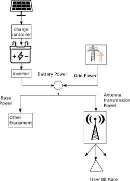
Figure 1: Solar Equipment

An important feature of solar power is that the energy production can vary widely over short periods of the order of an hour or less and these variations are unpredictable. A minimum amount of solar equipment is thus required to power a green base station. The main components are the solar panels and the battery bank. We also model the charge controllers needed to protect the batteries from overflowing and increase their lifetime. Finally, an AC-DC converter is also required to power the base station with DC current from its battery bank. Figure 1 shows the storage of solar energy into electrical energy as a back-up energy source to the electrical grid.

We use a solar profile to estimate the amount of electricity produced during the day since replacing the daily variation of sunlight by a single average value for the whole planning horizon would leave out the daily changes in sunlight. This profile is computed for an average day and assume that this is representative of the operation for the whole year.

This is clearly an over-simplification since the sunlight available can depend strongly on the season in regions far from the equator. First note that the illumination profile is defined for a year and that the actual length of a “year” is a parameter. The model can then easily be used to take into account the seasonal variations by taking a “year” as an actual season with the corresponding profile. The downside is that this makes the optimization problem larger and severely limits the size of networks that can be calculated by an IP solver.

What we have done instead was to use a single profile corresponding from a region in southern Morocco with abundant sunlight. Because one of our goals is to see if solar equipment proves in based on economics alone, this can be viewed as a most favorable case for solar. Since we found that using solar equipment is not economically justified with this optimistic profile, the same conclusion would hold under a more realistic profile.

III-A5 Cell Zooming

Cell zooming is a power control technique by which a base station can change its transmission power to match certain conditions. Decreasing the power of a given base station will decrease its coverage area but may increase that of neighboring ones by decreasing their SINR. Increasing the power has the opposite effect of increasing the coverage of the base station and potentially decreasing the QoS, and hence the coverage of neighbors. Implementing cell zooming is a complex issue that requires coordination between base stations and a knowledge of user demands. This is clearly outside of the scope of this paper.

Here, we assume that the network can operate within some specified bounds on the user coverage and QoS when all base stations transmit at their maximum power. This is the current mode of operation for networks that don’t use power management. Under this assumption, cell zooming can be modeled by introducing a state variable for the base stations. We assume that a given base station type has a certain number of power levels that it can use to transmit. The state variable indicates which of these levels is used at a given time. We also define a coverage variable that indicates whether a test point is covered by a base station in some state and add some constraints to make sure the coverage is logically consistent. The model then computes the best power levels and the corresponding coverage.

III-A6 Costs

The objective of the optimization model is to minimize the sum of capital and operating costs over the planning horizon. While it is true that an operator would be concerned by the net revenue produced by the network, in the present case, we assume that the network will always be able to meet the demand, independently of the decision to use solar energy or cell zooming. In other words, the revenue is independent of the choice of technology and can be ignored.

III-B Sets

Network management has to do with short-term decisions related to solar power, cell zooming and dynamic user assignment. These decisions are taken every day on a much shorter time scale than the planning decisions, typically a few hours. In this paper, we will use the term time to denote them.

The decisions to install base stations is taken on a much larger time scale, typically a year, and we will use the term year to denote these instants. The sets used in our model are defined in Table I.

$\mathcal{B}$	The set of base stations installed at the beginning of year 1. This is indexed by $j$.
$\mathcal{C}$	Set of candidate sites where new base stations can be installed. We can install at most one base station per candidate site. This is indexed by $j$.
$\mathcal{I}$	Set of test points. A test point represents the aggregated demand of a set of users, present or future. This is indexed by $i$.
$\mathcal{L}$	Set of base station types. This is indexed by $l$. Type $l=0$ corresponds to the base stations in $\mathcal{B}$.
$\mathcal{Q}$	The set of years that defines the planning horizon. This is indexed by $q=1\dots Q$. The traffic demand is defined at the beginning of each year and the planning decisions are made at that time.
$\mathcal{S}_{l}$	Set of states for base stations of type $l$. This is currently defined by the transmission power but the states could be used to model other operating conditions of the base stations. This is indexed by $s=0\dots S_{l}$.
$\mathcal{T}$	The time instants used to model the daily variation of traffic. This is indexed by $t=1\dots T$.

TABLE I: Sets

III-C Parameters Values

$B_{l,q^{\prime},q}^{+(-)}$	Maximum (minimum) amount of energy that can be stored in the battery of a base station of type $l$ installed in year $q^{\prime}$ and used in year $q>q^{\prime}$.
$C_{l,q}$	The installation cost of a base station of type $l\geq 1$ in year $q$. This is the undiscounted, nominal cost. This is made up of the construction cost, upkeep and software license costs. If the base station has solar equipment, this includes the cost of the system used for converting solar to electrical energy: solar panels, batteries, converters, inverters, etc.
$C^{G}_{j,q,t}$	Grid unit energy cost. This is the total charge per energy unit charged by the utilities company but excludes any emission cost that may be imposed by the regulators. We assume in the most general case that this can depend both on the time period, e.g., time-based grid rates, the base station, if the supplier of grid power has different rates in different regions and that it can change from one year to the next.
$E^{T}_{i,j,q,t}$	The energy needed by the station in site $j\in\mathcal{B}\cup\mathcal{C}$ to serve test point $i$ in period $t$ of year $q$.
$e_{l,q^{\prime},q,t}^{S}$	Amount of electrical energy produced by the solar panels in a base station of type $l$ during period $\Delta_{t}$ of year $q$ when these were installed in year $q^{\prime}<q$.
$k_{i,j,l,s,q,t}$	Indicator function for coverage. When set to 1, indicates that test point $i$ is in the coverage radius of base station of type $l$ installed on site $j\in\mathcal{B}\cup\mathcal{C}$ and using power level $W_{s},s\in S_{l}$ during period $\Delta_{t}$ of year $q$.
$m$	Number of installation periods per year.
$M_{l,j}$	Indicator function for base station installation. When set to 1, this indicates that a base station of type $l$ may be installed on candidate site $j$. By definition, $M_{0,j\in\mathcal{C}}=0$.
$q_{i}^{\ast}$	The first year when test point $i$ becomes active. This is used to model the growth of demand.
$r$	Discount rate.
$U_{l}$	Indicator function of solar equipment. When set to 1, this indicates that a base station of type $l$ has solar equipment. By definition, $U_{0}=0$.
$W_{l,s}$	Total power available to a base station of type $l$ in state $s$. By convention, for base stations that use cell zooming, $W_{l,0}$ is the power used when idle. For base stations that don’t use cell zooming, this is the given maximum used power. This includes the power used for serving the test points.
$W_{l,s}^{x}$	Transmission power used by a base station of type $l$ in state $s$. By convention, for base stations that use cell zooming, $W_{l,0}^{x}=0$. For base stations that don’t use cell zooming, this is the given maximum transmission power.
$\phi$	The number of days in an installation period.
$\Delta_{t}$	Length of the interval between time instants $t$ and $t-1$.
$\lambda_{k,q}$	Amount of greenhouse gasses emitted per unit energy produced, e.g., Mt/kWh, emitted by a source of type $k$, e.g., coal, gas, oil, etc.
$\pi_{q}$	Unit price per amount of greenhouse gasses emitted, e.g, $/Mt, in year $q$.
$\nu_{i,q}$	Indicator function for test point use. When set to 1, indicates that test point $i$ starts to be used. This is defined by $$\nu_{i,q}=\begin{cases}0&\text{ if $q<q^{\ast}_{i}$}\\ 1&\text{otherwise.}\end{cases}$$

TABLE II: Parameters

The parameters are defined in Table II. Note that we need the two year indices $q$ et $q^{\prime}$ to describe the use of solar equipments. For an equipment installed in year $q^{\prime}$, the energy production and storage capacity decrease over time so that they become less efficient as they grow older.

III-D Variables

In Table III we describe the decision variables, i.e., the quantities that are computed by the model. First, a number of decision variables that are set to 1 when the stated conditions hold.

$h_{i,j,q,t}$	Test point $i$ is assigned to site $j\in\mathcal{B}\cup\mathcal{C}$ in period $t$ of year $q$.
$u_{j,q,t}$	Solar batteries are used at site $j\in\mathcal{C}$ in period $t$ of year $q$.
$v_{l,s,j,q,t}$	The base station of type $l$ on site $j\in\mathcal{C}$ is in state $s$ in period $t$ of year $q$.
$z_{l,j,q}$	A base station of type $l$ is installed on candidate site $j\in\mathcal{C}$ in year $q$.

TABLE III: Decision variables

We also define some intermediate variables that can be computed from the parameters and decision variables. These will allow us to simplify the presentation of the optimization model and they also have a direct physical interpretation. They are presented in Table IV

$D_{j,q,t}$	The total amount of energy needed in a base station $j\in\mathcal{B}\cup\mathcal{C}$ in period $t$ of year $q$ by all test points currently served by the base station.
$\overline{E}_{j,q,t}^{P}$	Total amount of energy used by base station $j\in\mathcal{B}\cup\mathcal{C}$ during period $\Delta_{t}$ of year $q$ when operating from batteries.
$\overline{E}_{j,q,t}^{G}$	Total amount of energy used by base station $j\in\mathcal{B}\cup\mathcal{C}$ during period $\Delta_{t}$ of year $q$ when operating from the grid.
$E_{j,q,t}^{B}$	Energy available from the batteries of base station $j\in\mathcal{C}$ at the beginning of period $t$ of year $q$.
$E_{j,q,t}^{S}$	Energy produced by the solar panels of base station $j\in\mathcal{C}$ during period $t$ of year $q$.
$L_{j,q,t}$	Solar energy lost at base station $j\in\mathcal{C}$ during period $t$ of year $q$.
$w_{l,j,q}$	Indicator variable set to 1 if a base station of type $l$ is currently installed on site $j\in\mathcal{B}\cup\mathcal{C}$ in year $q$. This can be seen as the indicator of the state of site $j\in\mathcal{B}\cup\mathcal{C}$ in year $q$.

TABLE IV: Intermediate variables 1

We also need some intermediate variables to take into account the nonlinear terms that will show up in the model, they are defined in Table V.

$x_{l,s,j,q,t}$

Binary variable set to 1 if the base station of type $l$ that is installed at site $j\in\mathcal{C}$ operates in state $s$ using the batteries during period $t$ of year $q$. These variables are given by $x_{l,s,j,q,t}=v_{l,s,j,q,t}u_{j,q,t}$.

TABLE V: Intermediate variables 2

III-E Objective Function

The capital cost depends on the type of installed base stations and the installation year. Operating cost come from the grid cost for operating the base stations and the emission costs. Installing solar equipment can then allow a reduction in the operating cost, as well as a reduction of greenhouse gases, but at the expense of an increase in the capital cost. The objective function can then be written as:

$$\tiny Z=\sum_{q\in\mathcal{Q}}(1+r)^{-q}\sum_{j\in\mathcal{C}}\sum_{l\in\mathcal{L}}C_{l,j,q}z_{l,j,q}$$

$$+\sum_{q\in\mathcal{Q}}(1+r)^{-q}m\phi\sum_{j\in\mathcal{B}\cup\mathcal{C}}\sum_{t\in\mathcal{T}}\left\{C^{G}_{j,t}+\pi_{q}\lambda_{k,q}\right\}\overline{E}^{G}_{j,q,t}.$$ (1)

III-F Installation of Base Stations

We now describe the various constraints that may limit the installation of certain base stations in some sites.

First, some base station types might not be allowed on some sites because of physical or environmental conditions. This yield the constraint

$$\sum_{q\in\mathcal{Q}}z_{l,j,q}\leq M_{l,j}\qquad\forall l\in\mathcal{L},j\in\mathcal{C}.$$ (2)

Given that $M_{0,j\in\mathcal{C}}=0$, then if follows that $z_{0,j,q}=0\quad\forall j\in\mathcal{C},q\in\mathcal{Q}$. There is no replacement of base stations during the planning horizon so that a base station can be installed on a given site at most once, which yields the constraint

$$\sum_{l\in\mathcal{L},q\in\mathcal{Q}}z_{l,j,q}\leq 1\qquad\forall j\in\mathcal{C}.$$ (3)

If a base station is currently installed on some site at a given time, it must have been installed first at some previous time, so that

$$w_{l,j,q}=\sum_{q^{\prime}\leq q}z_{l,j,q^{\prime}}\qquad\forall l\in\mathcal{L},j\in\mathcal{C},q\in\mathcal{Q}.$$ (4)

In order for a base station to use solar energy, the type must have solar capability

$$u_{j,q,t}\leq\sum_{l\in\mathcal{L}}w_{l,j,q}U_{l}\qquad\forall j\in\mathcal{C},q\in\mathcal{Q},t\in\mathcal{T}.$$ (5)

III-G Test Point Assignment

All currently used test points must be assigned to a site:

$$\sum_{j\in\mathcal{B}\cup\mathcal{C}}h_{i,j,q,t}=\nu_{i,q}\qquad\forall i\in\mathcal{I},q\in\mathcal{Q},t\in\mathcal{T}.$$ (6)

The assignment is possible only if the coverage radius of the base station is large enough so that

$$h_{i,j,q,t} \leq\sum_{\begin{subarray}{c}l\in\mathcal{L}\geq 1\\ s\in\mathcal{S}_{l}\end{subarray}}v_{l,s,j,q,t}k_{i,j,l,s,q,t}$$

$$\forall i\in\mathcal{I},j\in\mathcal{C},q\in\mathcal{Q},t\in\mathcal{T}$$ (7)

$$h_{i,j,q,t} \leq\sum_{\begin{subarray}{c}l\in\mathcal{L}\\ s\in\mathcal{S}_{l}\end{subarray}}k_{i,j,l,s,q,t}$$

$$\forall i\in\mathcal{I},j\in\mathcal{B}\cup\mathcal{C},q\in\mathcal{Q},t\in\mathcal{T}.$$ (8)

III-H Energy Storage

The amount of energy available in a base station must be large enough to meet the demand for the test points that it serves

$$D_{j,q,t} =\sum_{i\in\mathcal{I}}E_{i,j,q,t}^{T}h_{i,j,q,t}$$

$$\forall j\in\mathcal{B}\cup\mathcal{C},q\in\mathcal{Q},t\in\mathcal{T}$$ (9)

$$D_{j,q,t} \leq\Delta_{t}W_{0,0}^{x}$$

$$\forall j\in\mathcal{B},q\in\mathcal{Q},t\in\mathcal{T}$$ (10)

$$D_{j,q,t} \leq\Delta_{t}\sum_{l\in\mathcal{L}\geq 1,s\in\mathcal{S}_{l}}v_{l,s,j,q,t}W_{l,s}^{x} \forall j\in\mathcal{C},q\in\mathcal{Q},t\in\mathcal{T}.$$ (11)

III-I Energy Production Model

The base station installed on some site $j$ must be in a single state for every period $t$ of year $q$. This is modelled by variable $w_{l,j,q}$. If a station of type $l$ has not yet been installed on site $j$ in year $q$, then $w_{l,j,q}=0\Rightarrow v_{l,s,j,q,t}=0\quad\forall s\in\mathcal{S}_{l}$. On the other hand, if type $l$ has already been installed, then $w_{l,j,q}=1$ which forces the selection of a single transmission power.

$$\sum_{s\in\mathcal{S}_{l}}v_{l,s,j,q,t}=w_{l,j,q}\qquad\forall l\in\mathcal{L},j\in\mathcal{C},q\in\mathcal{Q},t\in\mathcal{T}.$$ (12)

A base station must operate either in battery or grid mode but not both. This makes the model somewhat more complex. If we power the antennas from the batteries, we have to meet two conditons: the base station type that is currently installed must be of the right type and we must have decided to use battery power during that time. This yields:

$$\overline{E}_{j,q,t}^{P} =\Delta_{t}\sum_{l\in\mathcal{L}\geq 1,s\in\mathcal{S}_{l}}W_{l,s}v_{l,s,j,q,t}u_{j,q,t}$$

$$=\Delta_{t}\sum_{l\in\mathcal{L}\geq 1,s\in\mathcal{S}_{l}}W_{l,s}x_{l,s,j,q,t}~{}~{}~{}\forall j\in\mathcal{C},q\in\mathcal{Q},t\in\mathcal{T}$$ (13)

$$\overline{E}_{j,q,t}^{P} =0~{}~{}~{}\forall j\in\mathcal{B},q\in\mathcal{Q},t\in\mathcal{T}$$ . (14)

If we power from the grid, the conditions are that the right type of base station is installed and we have decided not to use battery power, i.e.,

$$\overline{E}^{G}_{j,q,t} =\Delta_{t}\sum_{l\in\mathcal{L}\geq 1,s\in\mathcal{S}_{l}}W_{l,s}v_{l,s,j,q,t}(1-u_{j,q,t})$$

$$=\Delta_{t}\sum_{l\in\mathcal{L}\geq 1,s\in\mathcal{S}_{l}}W_{l,s}(v_{l,s,j,q,t}-x_{l,s,j,q,t})$$

$$\forall j\in\mathcal{C},q\in\mathcal{Q},t\in\mathcal{T}$$ (15)

$$\overline{E}_{j,q,t}^{G} =\Delta_{t}W_{0,0}$$

$$~{}~{}\forall j\in\mathcal{B},q\in\mathcal{Q},t\in\mathcal{T}.$$ (16)

Note that both (13) and (16) introduce nonlinear terms in the model. This is taken care of in section III-J.

The energy produced by the solar equipments is defined by:

$${E}^{S}_{j,q,t}=\sum_{l\in\mathcal{L},q^{\prime}\in\mathcal{Q}}e_{l,q^{\prime},q,t}^{S}z_{l,j,q^{\prime}}\qquad\\ ~{}~{}~{}\forall j\in\mathcal{C},q\in\mathcal{Q},t\in\mathcal{T}.$$

The energy available at the beginning of period $t$ is given by:

$$E^{B}_{j,q,t} =E^{B}_{j,q,t-1}+E^{S}_{j,q,t-1}-L_{j,q,t-1}-\overline{E}^{P}_{j,q,t-1}$$

$$~{}~{}~{}\forall j\in\mathcal{C},q\in\mathcal{Q},t\in\mathcal{T}\geq 2$$ (17)

$$E^{B}_{j,q,1} =E^{B}_{j,q,T}+E^{S}_{j,q,T}-L_{j,q,T}-\overline{E}^{P}_{j,q,T}$$

$$~{}~{}~{}\forall j\in\mathcal{C},q\in\mathcal{Q}$$ (18)

The storage capacity of batteries is bounded above and below by:

$$\sum_{l\in\mathcal{L},q^{\prime}\in\mathcal{Q}}z_{l,j,q^{\prime}}B^{-}_{l,q^{\prime},q}\leq E^{B}_{j,q,t}\leq\sum_{l\in\mathcal{L},q^{\prime}\in\mathcal{Q}}z_{l,j,q^{\prime}}B_{l,q^{\prime},q}^{+}\qquad$$

$$~{}~{}~{}\forall j\in\mathcal{C},q\in\mathcal{Q},t\in\mathcal{T}$$ (19)

In a given period, a base station with solar equipment cannot lose more than the solar energy produced by the panels during this period:

$$0\leq L_{j,q,t}\leq E^{S}_{j,q,t}\qquad\forall j\in\mathcal{C},q\in\mathcal{Q},t\in\mathcal{T}$$ (20)

III-J Linearization

As written, the model contains nonlinear constraints due to the presence of the term $v_{l,s,j,q,t}u_{j,q,t}$ in (13) and (16). We can make the constraints linear by adding a set of independent variables $x_{l,s,j,q,t}=v_{l,s,j,q,t}u_{j,q,t}$ and adding the constraints:

$$x_{l,s,j,q,t} \leq v_{l,s,j,q,t}$$ (21)

$$x_{l,s,j,q,t} \leq u_{j,q,t}$$ (22)

$$x_{l,s,j,q,t} \geq v_{l,s,j,q,t}+u_{j,q,t}-1$$ (23)

$$\forall l\in\mathcal{L},s\in\mathcal{S}_{l},j \in\mathcal{C},q\in\mathcal{Q},t\in\mathcal{T}$$

IV Data Sets

In order for the results to be meaningful, we tried as best as possible to use realistic data for the costs and other technical parameters. The cost of a base station is made up of the building and installation cost in addition to the cost of the solar equipment. This is given by:

$$C_{l,q}=C^{B}_{l}+C^{S}_{q}$$ (24)

where

$C^{B}_{l}$ Construction and installation cost of a base station of type $l$ [45],

$C^{S}_{q}$ Purchase and installation cost of the solar equipment. This depends of the maximum power that can be generated and the battery storage cost. According to [46], a realistic value is 3$/W. This cost is indexed by year to model the expected decrease of the cost of solar generation.

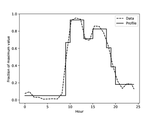
Figure 2: Traffic profile

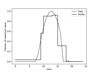
Figure 3: Illumination profile

The numerical results were computed for two small networks P1 and P2 with different peak traffic profiles. The parameters common to all cases are shown in Table VI. We have split the day into eight different periods to get a more accurate view of the changes in the user demands. These are shown on Figure 2. They correspond to a workday profile in an inner core cell [47].

The initial peak user rate for P1 is 10Mbps and grows at a 20% yearly rate so that user demand doubles every four years. The peak user rate for P2 is 12Mbps. We have used a 12% discount rate and a 2.64% inflation rate which reduces by half the value of a capital expenditure after 6 years. A unit cost of $0.20/kWh is representtive of the power rates in many countries. In Canada, for instance, this varies [48] from $0.07/kWh to $0.38/kWh for residential users. The cost of solar equipment is critical for the introduction of solar energy in networks. In northern countries, a realistic value [49] of $3/W is a threshold for having profitable solar power. In the numerical work, we have used the same cost over the whole planning horizon.

An antenna gain of 3 is typical for current antennas. The propagation coefficient and the channel noise are typical values for urban networks. Figure 3 shows the illumination profile for a city in southern Morocco [50]. The peak illumination is set to 800 $W/m^{2}$.

Parameter	Value
No periods	8
Discount rate	0.12
Inflation rate	0.0264
Annual demand growth rate	0.20
Unit cost of grid energy($/kWh)	0.20
Unit cost of solar equipment ($/w)	3
Antenna gain	3

TABLE VI: Common parameters for all networks

Pb No	No years	No Macro BS	No CS	No TP	Maximum initial user rate (Mbps)	Channel noise	Propagation coefficient
P1	10	1	8	18	10	$10^{-5}$	3
P2	10	1	14	30	12	$1.5e-5$	2

TABLE VII: Specific network parameters
BS: Base Station, CS: Candidate Sites, TP: Test Points

The parameters that vary for each network are shown on Table VII. They define the size of each problem. All cases are for a 10-year horizon. This value was chosen as a compromise between having a problem size small enough to be able to solve it in reasonable time and having a large enough horizon to allow significant discounting and installation delays.

The macro base stations are the ones currently in the operator’s network. We use only one of these so that the candidate sites will be needed to meet the demand. We limit the study to small networks because we want to compare the total cost for different scenarios. For this to be meaningful, we need to compute optimal solutions or at least solutions with a small gap. This can be done in a reasonable execution time only for small networks.

V Scenarios

The options that are compared are summarized in a number of scenarios.

B: Base Network

This is the reference network. It has no solar equipment, no cell zooming and no dynamic management. It corresponds to most of the base stations currently used in 4G networks.

S: Solar Power

In this scenario, only solar is enabled so that we can quantify the savings from solar power. One goal is to try to determine a relationship between the unit cost of solar power on the one hand and the capital cost of the solar equipment and the grid cost on the other. We also want to see, in the case where the unit cost of solar is smaller than the grid cost, whether the best solution is to install solar equipment everywhere.

O: On-OFF

In this scenario, only the BS sleeping mode is enabled, when a base station can be put on idle power during a low traffic period. This is a special case of cell zooming.

Z: Cell Zooming

Here, only cell zooming is enabled. With cell zooming, we can increase the reach of base stations in a given direction while reducing it elsewhere. We can then evaluate the impact of cell zooming on the network cost. This will be reflected by a reduction of the operating costs and may have an impact on the capital cost.

S+O: Solar and On-off

This is a combination between scenario S and scenario On-OFF where both technologies are used at the same time. This will allow us to see whether the benefits of the two technologies add up.

S+Z: Solar and Cell Zooming

In this scenario, both solar and cell zooming are available. This is the most important one, because it optimizes the dynamic management and the use of the solar together to achieve a truly optimal solution.

S + Z0

Here, both solar and cell zooming are available but can be installed only in the first year. This corresponds to a planning technique that does not consider the time evolution of the network, as was done in [37].

FS + Z

This scenario is used to compare a solution where we force the installation of solar equipment on all BS. That case is interesting to know if a purely solar solution gives reduced costs and if not, how sub-optimal it is.

These scenarios are implemented in the model by fixing different variables at zero while leaving the others free. This is summarized in Table V. For simplicity and brevity, we only illustrate solutions to the peak period the last year which corresponds to the peak of demand for TP on the planning horizon. Any feasible solution at this time is also feasible for all other periods.

Scnr	S	O	Z	$z$	$v$	$u$	$h$
B	no	no	no	F	0	0	F
S	yes	no	no	F	0	F	F
O	no	yes	no	F	***	0	F
Z	no	yes	yes	F	0	0	F
S+O	yes	yes	no	F	***	F	F
S+Z	yes	yes	yes	F	0	F	F
S+Z0	yes	yes	yes	*	0	F	F
FS+Z	yes	yes	yes	**	F	F	F

TABLE VIII: State of variables for each Scenario: *: Free in first year only **: Only solar types allowed ***: Two states only. F: variable is free

VI Numerical Results

In this part, we analyze the results from the optimization model with and without GHG taxes. We use two small networks, P1 and P2, generated from the same data except for channel noise, propagation coefficient and the demand with low values for network P1 and high for P2.

In order to produce optimal solutions, the problem and its variants are modeled by AMPL and solved using CPLEX with the default options. AMPL integrates pre-solving mechanisms which allow certain variables and constraints to be eliminated before calling on the solver. We used a standard IP solver because we must have an exact solution for all scenarios in order to compare the costs of solar and sleep modes. Larger networks will require heuristic techniques specifically adapted to the optimization model. The algorithms were executed on Intel(R) Core(TM) i7-8700 CPU $@$ 3.20GHz with 12 cores running at 3.5 GHz and 65 GBs RAM.

Tables V and V give various costs and amounts of energy for the two networks without GHG taxes. The column titles represent

$Z$

Total network cost. This is the sum of $Z_{c}$ and $Z_{op}$

$\Delta$

Change in $Z$ relative to the cost of scenario B

$Z_{c}$

Total capital cost including solar equipment

$Z_{s}$

Capital cost of solar equipment

$Z_{op}$

Operating cost

$Z_{g}$

Cost of grid energy

$Z_{CO_{2}}$

Cost of greenhouse taxes

$Z_{s}$/kWh

Production cost of solar energy = $Z_{s}$/(Total energy produced by the panels)

$Z_{s}^{\ast}$/kWh

Production cost for the energy used. This is $Z_{s}$/(Total energy used by the network)

The second set of tables V and V shows energy information where all energy values are in MWh. The column labels are defined as

$E_{N}$

This is the total amount of energy that the network needs

$E_{G}$

The amount of energy coming from the grid

CO₂

The number of tons of CO2 produced by the network

$E_{si}$

The amount of energy produced by the installed solar equipment

$E_{su}$

This is the amount of solar energy effectively used

The difference $E_{si}-E_{su}$ is the energy lost due to the limited capacity of batteries. The $Z_{s}$/kWh column gives the cost in dollars per kilowatt-hour of solar based on the amount of solar energy actually used. This is simply the value of the CAPEX column divided by the solar energy used. The $Z_{s}^{\ast}$/kWh column is the energy lost due to the limited capacity batteries. Solar losses are the ratio $(E_{si}-E_{su})/E_{si}$. This ratio clearly shows that installing too much solar equipment will increase losses and installing larger batteries is too expensive.

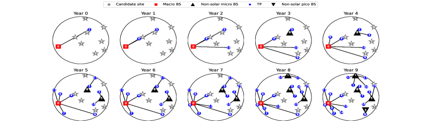
Figure 4: Network P1 (Without taxes and Scenario S+Z)

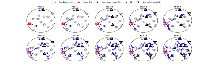
Figure 5: Network P2 (Without taxes and Scenario S+Z)

VI-A Without taxes

In this part, we do not consider emissions taxes. Our objective is to see if free market economics can drive the introduction of solar BSs to reduce GHG emissions. Figures 4 and 5 show the base station installation planning for the S+Z scenario for P1 and P2 without taxes. One can also see the assignment of each of the TPs to BSs every year. The growing demand over the years requires the installation of new stations. It turns out that the optimal solution is not to install solar base stations both for low and high traffic. This is due to the current high costs of solar equipment and also to the cost of batteries replacement. Batteries for green micro BSs have a lifetime of 7 years and 5 years for green pico BSs. This is less than the planning horizon so that the batteries have to be replaced. It then turns out that with the current grid prices, the traditional BSs system is less expensive so that even over a 10-year horizon, the installation of stations that run on solar energy is not justified.

This can be seen by comparing the results of Table V for the scenarios S+Z and FS+Z. In the second case, we force the installation of solar equipment on all base stations. For P1, this reduces the operating cost $Z_{o}$ from 17.2 to 16.3 with a saving of 0.9 while the capital cost of solar equipment $Z_{s}$ increases from 21.16 to 23.8 for an added expense of 2.64, larger than the savings on the operating cost. The same results can be found for P2, where the savings is 5.7 and the added cost, 7.4. The corresponding results of Table V also show that forcing the use of solar will have a significant impact on CO2 emissions.

It should be noted that while solar stations do not emit CO2, there is still some amount of CO2 emissions in the Full S + Z scenario. We assumed that the system already includes non-solar macro stations BSs that still produce emissions because of their large energy use.

If we consider only GHG emissions, PV-Battery BSs, which produce no GHG, are very attractive as compared with traditional BSs. When we take into account realistic cost data, as we do here, the investment in solar equipment is not profitable for cellular operators. The size of the batteries and PV needed to reduce the GHG emissions is such that this increases the price of the solar equipment and thus the total CAPEX above that for non-solar networks.

Even if solar base stations are not viable, we can also see from scenario Z that cell zooming by itself can reduce the CO2 emissions and the operating cost, with a net saving on the total cost. Thus cell zooming is a good compromise compared with the Full S+Z scenario.

TABLE IX: Results without taxes (Costs)

TABLE X: Results without taxes (Energy).

VI-B With taxes

In this section, we study how a GHG tax can improve the the environmental impact of the network. A GHG tax on fuels is set at a price of $50 per ton of ECO2 in the first year and increased by $50 each year until it reaches $500 in the 10th year. We consider that coal is the source of electricity and that 1 kWh of coal-produced electricity emits 1 kg ECO2.

We arrived at the tax growth formula by a trial-and-error procedure. We started with a constant value of $50, the carbon tax for 2022 [51] in Canada. Initial results showed that this was not large enough to yield solutions with green BSs. We then tried small progressive increases from this value, without success. We finally found that the carbon tax had to increase by a factor of ten over the planning horizon to produce solutions with green BSs, which is an important finding of this project.

TABLE XI: Results with taxes (Costs)

TABLE XII: Results with taxes (Energy)

Table V and V list the cost and energy when GHG taxes are considered. We can see that the total costs are increased both for P1 and P2 due to the rise of the OPEX. In most scenarios, when solar is enabled, it is used in the planning. We can also notice a reduction of 47 tons of C02 emissions for P1 and 118 tons for P2.

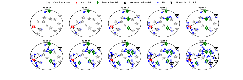
Figure 6: Network P2(With taxes and Scenario S)

Figure 7: Network P2(With taxes and Scenario S+Z)

As we have seen from the cost tables, the largest part of the total capital cost comes from the installation of the base stations themselves while the operating cost is only a small fraction of this total. We can see an important result from Figures 6 and 7. Both scenarios produce basically the same sequence of base station installations with the single exception of base station 9 in year 6. In the S scenario with only the solar option, the optimal solution is to install a solar micro base station. If we allow cell zooming, however, we need only to install a non-solar micro base station. Because the solar cost is relatively large, this produces a significant decrease in the capital cost of solar equipment, from 8.1 to 5.1. In other words, the introduction of cell zooming can reducee not only the operating cost, as expected, but also the capital cost, in the present case by choosing a less expensive equipment. It is quite conceivable that in other cases, this might lead to actually postponing a capital expense with a large reduction in the total cost.

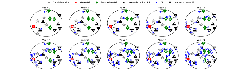
Figure 8: Network P2(With taxes and Scenario S + Z + Z free at year 0 )

We can also see why a static model like S+Z0, where the decision is taken only at the beginning of the study period, can produce such costly solutions. From Figure 8, we see that a large number of base stations are installed at period 0 but are not used until (much) later.

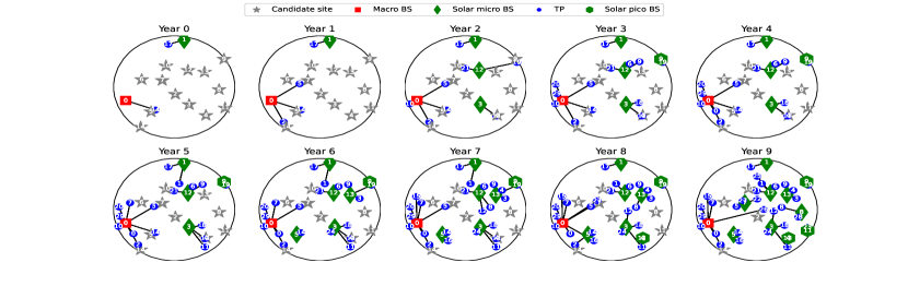
Figure 9: Network P1(With taxes and Scenario Full S + Z)

We can also see from Figure 9 why scenario FS+Z, where solar is installed everywhere in network P2, is more expensive. All the non-solar base stations that were installed in the S+Z scenario are now forced to be solar which is where the cost increase comes from.

VI-C Daily Assignment of TPs to BS

We can examine in some detail the TP assignment to the BS for P1 and the S+Z scenario. We see that the dynamic assignment of test points to base stations uses sleep mode in an optimal way in each period to reduce both the OPEX and CAPEX.

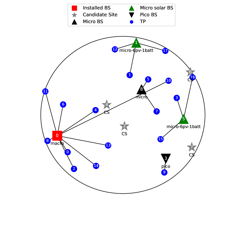
Figure 10: Assignment of TPs at 10:00

Figure 10 shows the dynamics of the network with the peak traffic demand at period 10:00.

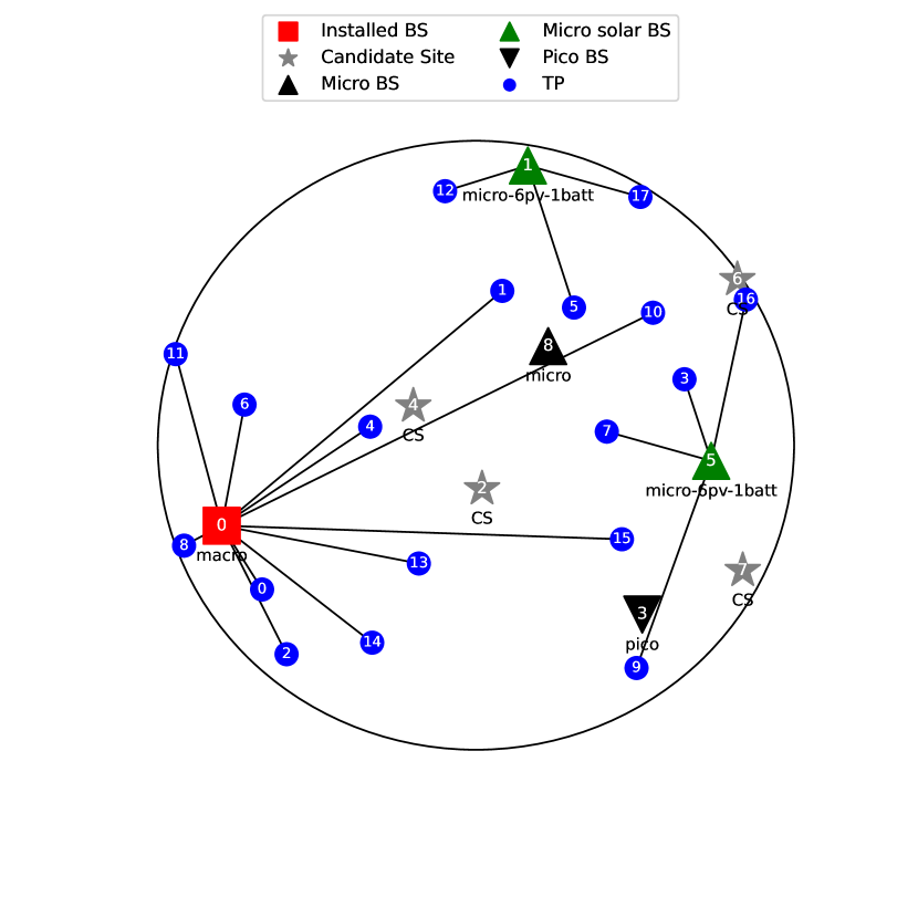
Figure 11: Assignment of TPs at 13:00

We see on Figure 11 that base stations 3 and 5 are in standby mode at 13:00.

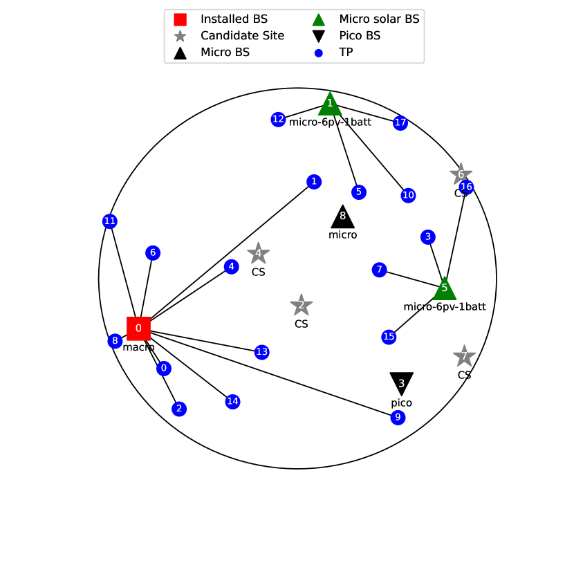
Figure 12: Assignment of TPs at 15:00

At 15:00, BS 3 is in standby mode in Figure 12.

VII Conclusions

With the advent of 5G and beyond, there will be a significant increase in energy use and green gas emissions in cellular networks. A potential solution is to use solar-powered base stations in the access in addition to other energy management techniques.

In this article, we propose a comprehensive optimization model that not only shows the technical integration of solar power with other management features, but also allows an in-depth study of its economics. The objective is to reduce the total cost, including CAPEX and OPEX, over a ten-year horizon and under constraints that reflect the inter-relation between networking and energy. Our aim is to study the viability of green networks in reducing costs and GHGs. We use data that is as realistic as possible to study the technical and economic interactions.

We found that cellular zooming offers an effective solution for reducing planning and operating costs in a cellular network. We also found that cell zooming can not only reduce operating costs but also capital costs by avoiding the installation of expensive solar stations. However, in terms of greening future networks, we found that current energy and solar-related equipment prices are such that green base stations are not economically viable for cellular operators.

We then added a high and progressive carbon tax to the model. This produced networks where the CO2 emissions were drastically reduced as green base stations were added into the planning. A conclusion is that unless there is a significant reduction in the cost of solar equipment, some form of carbon tax will be needed and that that tax has to be significantly higher than current values.

Appendix A Demand Model

The main requirement from users is generally expressed in terms of the bit rate of a connection. In our model, demand is expressed in terms of $E^{T}_{i,j,q,t}$, the energy required by the base station to serve a user so that the demand in bit rate needs to be converted into an energy demand.

This in turn is related to the notion of coverage. In current networks, where base stations are always turned on at a fixed power, we can define a fixed coverage radius for a given bit rate to the users. With cell zooming and the ensuing dynamic user allocation, the coverage radius is no longer a fixed base station parameter but now depends on the transmission power of the base station at some instant.

In this section, we provide a simple model for this extended coverage radius concept and also a transformation rule from a demand in bit rates into an energy demand. This model is more realistic than the one used in [37] where these values were generated randomly.

A-A Coverage

In order to model the coverage, we assume and additive, white noise channel. This could easily extended to more complex models if needed. In that case, the maximum bit rate $\overline{\rho}_{i,j,l,s}$ that a test point $i$ can receive from a base station $j$ of type $l$ transmitting at the power level of state $s$ is given by

$$\overline{\rho}_{i,j,l,s}=B_{l}\log_{2}\left(1+\frac{W^{r}_{i,j,l,s}}{N}\right)$$ (25)

where

$B_{l}$ The bandwidth of the channels used by a base station of type $l$

$W^{r}_{i,j,l,s}$ The power received by the test point

$N$ The channel noise.

A base station can meet a required bit rate $\rho_{i,q,t}$ from a test point $i$ at time $t$ from year $q$ if $\rho_{i,q,t}\leq\overline{\rho}_{i,j,l,s}$. From this, we can define the generalized coverage parameter ${\mathbf{k}}$ for each time instant by the condition.

$$k_{i,j,l,s,q,t} =\begin{cases}1&\text{if $\rho_{i,q,t}\leq\overline{\rho}_{i,j,l,s}$}\\ 0&\text{otherwise}\end{cases}$$ (26)

$$\forall\,i\in\mathcal{I},\ \ j\in\mathcal{B\cup C},\ l\in\mathcal{L},\ s\in\mathcal{S}_{l},\ q\in\mathcal{Q},\ t\in\mathcal{T}.$$

A-A1 Channel Gain

The signal power received by a test point from a base station transmitting at a given power is given by

$$W^{r}_{i,j,l,s} =W^{x}_{l,s}\gamma_{i,j}$$ (27)

$$\gamma_{i,j} =\frac{\alpha}{d_{i,j}^{n}}$$ (28)

where

$W^{x}_{i,j,l,s}$

is the base station transmission power

$W^{r}_{i,j,l,s}$

is the power received at the test point

$d_{i,j}$

the distance between $i$ and $j$

$n$

the propagation coefficient.

$\alpha$

the antenna gain

A-A2 Energy Demand

We can now compute the power required from a base station by a test point by replacing (27) and (28) into (25) and solving for $W^{x}_{i,j,q,t}$ to get

$$W^{x}_{i,j,q,t}=\frac{Nd_{i,j}^{n}}{\alpha}\left(2^{\rho_{i,q,t}/B_{j}}-1\right)$$ (29)

so that the energy requirement during period $(q,t)$ is given by

$$E^{T}_{i,j,q,t}=\Delta tW^{x}_{i,j,q,t}$$ (30)

References

- [1] A. Bohli and R. Bouallegue, “How to meet increased capacities by future green 5G networks: A survey,” IEEE Access, vol. 7, pp. 42 220–42 237, 2019.
- [2] V. Chamola and B.Sikdar, “Solar powered cellular base stations:current scenario, issues and proposed solutions,” IEEE Communications Magazine, pp. 108–114, may 2016.
- [3] J. Malmodin and D. Lundén, “The energy and carbon footprint of the global ict and e&m sectors 2010–2015,” Sustainability, vol. 10, no. 9, 2018. [Online]. Available: https://www.mdpi.com/2071-1050/10/9/3027
- [4] C. Freitag, M. Berners-Lee, K. Widdicks, B. Knowles, G. S. Blair, and A. Friday, “The real climate and transformative impact of ict: A critique of estimates, trends, and regulations,” Patterns, vol. 2, no. 9, p. 100340, 2021. [Online]. Available: https://www.sciencedirect.com/science/article/pii/S2666389921001884
- [5] A. Israr, Q. Yang, W. Li, and A. Y. Zomaya, “Renewable energy powered sustainable 5g network infrastructure: Opportunities, challenges and perspectives,” Journal of Network and Computer Applications, vol. 175, p. 102910, 2021. [Online]. Available: https://www.sciencedirect.com/science/article/pii/S1084804520303702
- [6] L. Williams, B. K. Sovacool, and T. J. Foxon, “The energy use implications of 5g: Reviewing whole network operational energy, embodied energy, and indirect effects,” Renewable and Sustainable Energy Reviews, vol. 157, p. 112033, 2022. [Online]. Available: https://www.sciencedirect.com/science/article/pii/S1364032121012958
- [7] G. Wu, C. Yang, S. Li, and G. Y. Li, “Recent advances in energy-efficient networks and their application in 5g systems,” IEEE Wireless Communications, vol. 22, no. 2, pp. 145–151, 2015.
- [8] G. Ancans, V. Bobrovs, A. Ancans, and D. Kalibatiene, “Spectrum considerations for 5G mobile communication systems,” Procedia Computer Science, vol. 104, pp. 509–516, 2017, iCTE 2016, Riga Technical University, Latvia. [Online]. Available: https://www.sciencedirect.com/science/article/pii/S1877050917301679
- [9] S. Hu, X. Chen, W. Ni, X. Wang, and E. Hossain, “Modeling and analysis of energy harvesting and smart grid-powered wireless communication networks: A contemporary survey,” IEEE Transactions on Green Communications and Networking, vol. 4, no. 2, pp. 461–496, 2020.
- [10] “Cost of electricity by source.” [Online]. Available: https://en.wikipedia.org/wiki/Cost_of_electricity_by_source
- [11] M. H. Alsharif, R. Nordin, and M. Ismail, “Energy optimisation of hybrid off-grid system for remote telecommunication base station deployment in Malaysia,” EURASIP Journal on Wireless Communications and Networking, vol. 2015, no. 1, p. 64, Mar 2015. [Online]. Available: https://doi.org/10.1186/s13638-015-0284-7
- [12] O. M. Babatunde, I. H. Denwigwe, D. E. Babatunde, A. O. Ayeni, T. B. Adedoja, and O. S. Adedoja, “Techno-economic assessment of photovoltaic-diesel generator-battery energy system for base transceiver stations loads in Nigeria,” Cogent Engineering, vol. 6, no. 1, p. 1684805, 2019. [Online]. Available: https://doi.org/10.1080/23311916.2019.1684805
- [13] F. Odoi-Yorke and A. Woenagnon, “Techno-economic assessment of solar pv/fuel cell hybrid power system for telecom base stations in Ghana,” Cogent Engineering, vol. 8, no. 1, p. 1911285, 2021. [Online]. Available: https://doi.org/10.1080/23311916.2021.1911285
- [14] B. A. Aderemi, S. P. D. Chowdhury, T. O. Olwal, and A. M. Abu-Mahfouz, “Techno-economic feasibility of hybrid solar photovoltaic and battery energy storage power system for a mobile cellular base station in Soshanguve, South Africa,” Energies, vol. 11, no. 6, 2018. [Online]. Available: https://www.mdpi.com/1996-1073/11/6/1572
- [15] M. W. Baidas, R. W. Hasaneya, R. M. Kamel, and S. S. Alanzi, “Solar-powered cellular base stations in Kuwait: A case study,” Energies, vol. 14, no. 22, 2021. [Online]. Available: https://www.mdpi.com/1996-1073/14/22/7494
- [16] M. H. Alsharif, R. Kannadasan, A. Jahid, M. A. Albreem, J. Nebhen, and B. J. Choi, “Long-term techno-economic analysis of sustainable and zero grid cellular base station,” IEEE Access, vol. 9, pp. 54 159–54 172, 2021.
- [17] I. A. Ibrahim, S. Sabah, R. Abbas, M. Hossain, and H. Fahed, “A novel sizing method of a standalone photovoltaic system for powering a mobile network base station using a multi-objective wind driven optimization algorithm,” Energy Conversion and Management, vol. 238, p. 114179, 2021. [Online]. Available: https://www.sciencedirect.com/science/article/pii/S0196890421003551
- [18] D. Niyato, X. Lu, and P. Nanyang, “Adaptive power management for wireless base stations in a smart grid environment,” IEEE Wireless Communications, vol. 19, no. 6, pp. 44–51, Dec. 2012.
- [19] L. Liu, S. Men, M. Liu, and B. Zhou, “An energy saving solution for wireless communication equipment,” in IEEE 36th International Telecommunications Energy Conference (INTELEC), 2014, pp. 1–3.
- [20] S. Herrería-Alonso, M. Rodríguez-Pérez, M. Fernández-Veiga, and C. López-García, “An optimal dynamic sleeping control policy for single base stations in green cellular networks,” Journal of Network and Computer Applications, vol. 116, pp. 86–94, 2018. [Online]. Available: https://www.sciencedirect.com/science/article/pii/S1084804518301760
- [21] S. Boiardi, A. Capone, and B. Sansó, “Joint design and management of energy-aware mesh networks,” Ad Hoc Networks, vol. 10, no. 7, pp. 1482–1496, 2012. [Online]. Available: https://www.sciencedirect.com/science/article/pii/S1570870512000765
- [22] S. Mollahasani and E. Onur, “Density-aware, energy- and spectrum-efficient small cell scheduling,” IEEE Access, vol. 7, pp. 65 852–65 869, 2019.
- [23] A. Jahid, M. Hossain, M. Monju, M. Rahman, and M. Hossain, “Techno-economic and energy efficiency analysis of optimal power supply solutions for green cellular base stations,” IEEE Access, vol. 8, pp. 43 776–43 795, 2020.
- [24] X. Xu, C. Yuan, W. Chen, X. Tao, and Y. Sun, “Adaptive cell zooming and sleeping for green heterogeneous ultradense networks,” IEEE Transactions on Vehicular Technology, vol. 67, no. 2, pp. 1612–1621, 2018.
- [25] D. Tipper, A. Rezgui, P. Krishnamurthy, and P. Pacharintanakul, “Dimming cellular networks,” in IEEE GLOBECOM, 2010, pp. 1–6.
- [26] L. Budzisz, F. Ganji, G. Rizzo, M. A. Marsan, M. Meo, Y. Zhang, G. Koutitas, L. Tassiulas, S. Lambert, B. Lannoo, M. Pickavet, A. Conte, I. Haratcherev, and A. Wolisz, “Dynamic resource provisioning for energy efficiency in wireless access networks: A survey and an outlook,” IEEE Communication Surveys & Tutorials, vol. 16, no. 4, pp. 2259–2285, 2014.
- [27] W. Vereecken, W. V. Heddeghem, M. Deruyck, B. Puype, B. Lannoo, W. Joseph, D. Colle, L. Martens, and P. Demeester, “Power consumption in telecommunication networks: overview and reduction strategies,” Communications Magazine, vol. 49, no. 6, pp. 62–69, 2011.
- [28] J. Wu, Y. Zhang, M. Zukerman, and E. K.-N. Yung, “Energy-efficient base-stations sleep-mode techniques in green cellular networks: A survey,” Communication Surveys & Tutorials, vol. 17, no. 2, pp. 803–826, 2015.
- [29] Y. Wu, H. Gaoning, S. Zhang, Y. Chen, and S. Xu, “Energy efficient coverage planning in cellular networks with sleep mode,” in Proc. IEEE 24th International Symposium on Personal, Indoor and Mobile Radio Communications, Sep. 2013, pp. 2586–2590.
- [30] D. Tsilimantos, J. Gorce, and E. Altman, “Stochastic analysis of energy savings with sleep mode in OFDMA wireless networks,” in Proceedings IEEE INFOCOM. IEEE, 2013, pp. 1097–1105. [Online]. Available: https://dx.doi.org/10.1109/INFCOM.2013.6566900
- [31] L. Chiaraviglio, D. Ciullo, M. Meo, and M. Marsan, “Energy-aware UMTS access networks,” in WPMC’08, 2008.
- [32] Z. Niu, Y. Wu, J. Gong, and Z. Yang, “Cell zooming for cost-efficient green cellular networks,” Communications Magazine, vol. 48, no. 11, pp. 74–79, Nov. 2010.
- [33] M. Yigitel, O. Incel, and C. Ersoy, “Dynamic base station planning with power adaptation for green wireless cellular networks,” Eurasip Journal on Wireless Communications and Networking, vol. 2014, no. 1, p. 77, 2014. [Online]. Available: https://dx.doi.org/10.1186/1687-1499-2014-77
- [34] B. Wang, Q. Yang, L. T. Yang, and C. Zhu, “On minimizing energy consumption cost in green heterogeneous wireless networks,” Computer Networks, vol. 129, pp. 522–535, Dec. 2017. [Online]. Available: https://doi.org/10.1016/j.comnet.2017.03.024
- [35] S. Boiardi, A. Capone, and B. Sansò, “Radio planning of energy-aware cellular networks,” Computer Networks, vol. 57, pp. 2564–2577, 2013.
- [36] ——, “Planning for energy-aware wireless networks,” IEEE Communications Magazine, vol. 52, no. 2, pp. 156–162, Feb. 2014.
- [37] M. D’Amours, A. Girard, and B. Sansò, “Planning solar in energy-managed cellular networks,” IEEE Access, vol. 6, pp. 65 212–65 226, Oct. 2018.
- [38] O. Arnold, F. Richter, G. Fettweis, and O. Blume, “Power consumption modeling of different base station types in heterogeneous cellular networks,” in Future Network Mobile Summit, 2010, pp. 1–8.
- [39] H. Claussen, I. Ashraf, and L. T. W. Ho, “Dynamic idle mode procedures for femtocells,” Bell Labs Technical Journal, vol. 15, no. 2, pp. 95–116, 2010. [Online]. Available: https://onlinelibrary.wiley.com/doi/abs/10.1002/bltj.20443
- [40] Y. Zhang, M. Meo, R. Gerboni, and M. A. Marsan, “Minimum cost solar power systems for LTE macro base stations,” Computer Networks, vol. 112, pp. 12–23, Oct. 2017.
- [41] A. Balakrishnan, S. De, and L.-C. Wang, “Network operator revenue maximization in dual powered green cellular networks,” IEEE Transactions on Green Communications and Networking, vol. 5, no. 4, pp. 1791–1805, 2021.
- [42] M. Zheng, P. Pawelczak, S. Stanczak, and H. Yu, “Planning of cellular networks enhanced by energy harvesting,” IEEE Communications Letters, vol. 17, no. 6, pp. 1092–1095, 2013.
- [43] Y. Chen, L. Duan, and Q. Zhang, “Financial analysis of network upgrade,” IEEE Transactions on Vehicular Technology, vol. 67, no. 6, pp. 5496–5499, 2018.
- [44] J. Xu, L. Duan, and R. Zhang, “Cost-aware green cellular networks with energy and communication cooperation,” IEEE Communications Magazine, pp. 257–263, may 2015.
- [45] K. Johansson, A. Furuskar, P. Karlsson, and J. Zander, “Relation between base station characteristics and cost structure in cellular systems,” in 15th International Symposium on Personal, Indoor and Mobile Radio Communications (PIMRC), Barcelona, Spain, Sep. 2004, pp. 2627–2631. [Online]. Available: https://ieeexplore.ieee.org/abstract/document/1368795
- [46] “Cost and performance characteristics of new generating technologies, annual energy outlook 2021,” Feb. 2021. [Online]. Available: https://www.eia.gov/outlooks/aeo/assumptions/pdf/table_8.2.pdf
- [47] M. Marsan, G. Bucalo, A. Di Caro, M. Meo, and Y. Zhang, “Towards zero grid electricity networking: Powering BSs with renewable energy sources,” in IEEE International Conference on Communications Workshops, Jun. 2013, pp. 596–601.
- [48] R. Urban, “Electricity prices in Canada,” 2021. [Online]. Available: https://www.energyhub.org/electricity-prices/
- [49] Hydro-Québec. (2019) Costs and affordability: Don’t be blinded by the (sun)light! [Online]. Available: https://www.hydroquebec.com/solar/costs.html
- [50] “Rayonnement solaire à Ouarzazate.” [Online]. Available: https://fr.tutiempo.net/radiation-solaire/ouarzazate.html
- [51] Ministry of Environment and Climate Change Strategy, “British Columbia’s carbon tax,” 2022. [Online]. Available: https://www2.gov.bc.ca/gov/content/environment/climate-change/clean-economy#carbontax