i-MAE: Are Latent Representations in Masked Autoencoders Linearly Separable?

Abstract

Masked image modeling (MIM) has been recognized as a strong and popular self-supervised pre-training approach in the vision domain. However, the interpretability of the mechanism and properties of the learned representations by such a scheme are so far not well-explored. In this work, through comprehensive experiments and empirical studies on Masked Autoencoders (MAE), we address two critical questions to explore the behaviors of the learned representations: (i) Are the latent representations in Masked Autoencoders linearly separable if the input is a mixture of two images instead of one? This can be concrete evidence used to explain why MAE-learned representations have superior performance on downstream tasks, as proven by many literature impressively. (ii) What is the degree of semantics encoded in the latent feature space by Masked Autoencoders? To explore these two problems, we propose a simple yet effective Interpretable MAE (i-MAE) framework with a two-way image reconstruction and a latent feature reconstruction with distillation loss to help us understand the behaviors inside MAE’s structure. Extensive experiments are conducted on CIFAR-10/100, Tiny-ImageNet and ImageNet-1K datasets to verify the observations we discovered. Furthermore, in addition to qualitatively analyzing the characteristics of the latent representations, we examine the existence of linear separability and the degree of semantics in the latent space by proposing two novel metrics. The surprising and consistent results across the qualitative and quantitative experiments demonstrate that i-MAE is a superior framework design for interpretability research of MAE frameworks, as well as achieving better representational ability. 

1 Introduction

Self-supervised learning aims to learn representations from abundant unlabeled data for benefiting various downstream tasks. Recently, many self-supervised approaches have been proposed in the vision domain, such as pre-text based methods (Doersch et al., 2015; Zhang et al., 2016; Gidaris et al., 2018), contrastive learning with Siamese networks (Oord et al., 2018; He et al., 2020; Chen et al., 2020; Henaff, 2020), masked image modeling (MIM) (He et al., 2022; Bao et al., 2022; Xie et al., 2022), and etc. Among them, MIM has shown a preponderant advantage in performance, and the representative method Masked Autoencoders (MAE) (He et al., 2022) has attracted much attention in the field. A natural question is then raised: Where is the benefit of the transferability to downstream tasks from in MAE-based training? This motivates us to develop a framework to shed light on the reasons for the superior latent representation from MAE. Also, as the interpretability of the MAE framework is still under-studied in this area, it is crucial to explore this in a specific and exhaustive way.

Intuitively, a good representation should be separable and contain enough semantics from its input, so that it can have a qualified ability to distinguish different classes with better performance on downstream tasks. Nonetheless, how to evaluate the separability and the degree of semantics on the latent features is not clear thus far. Moreover, the mechanism of an Autoencoder compressing the information from input by reconstructing itself has been a well-established self-supervised learning architecture, but the explanation of the features learned from such approaches is still under-explored.

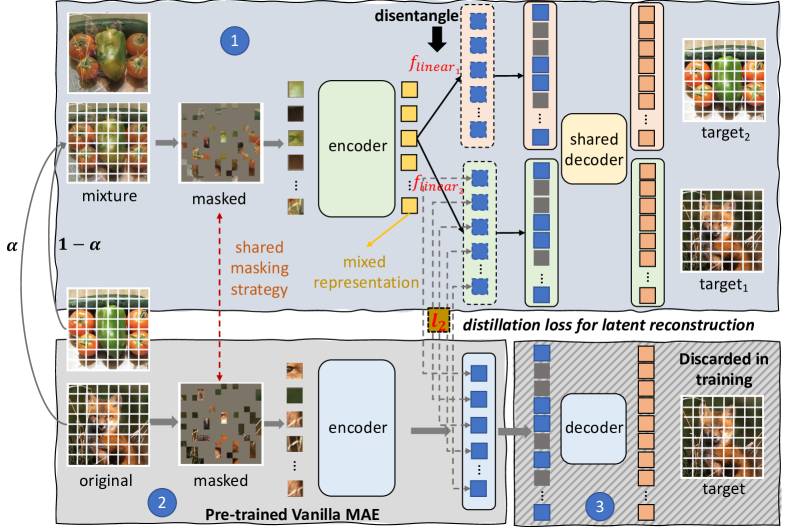
To address the difficulties of identifying separability and semantics in latent features, we first propose a novel framework, i-MAE, upon vanilla MAE. It consists of a mixture-based masked autoencoder branch for disentangling the mixed representations by linearly separating two different instances, and a pre-trained vanilla MAE as the guidance to distill the disentangled representations. An illustration of the overview framework architecture is shown in Fig. 2. This framework is designed for answering two interesting questions: (i) Are the latent representations in Masked Autoencoders linearly separable? (ii) What is the degree of semantics encoded in the latent feature space by Masked Autoencoders? These two questions can reveal the fact that MAE learned features are good at separating different classes. We attribute the superior representation of MAE to it learning separable features for downstream tasks with enough semantics.

In addition to qualitative studies, we also develop two metrics to address the two questions quantitatively. In the first metric, we employ $\ell_{2}$ distance from high-dimensional Euclidean spaces to measure the similarity between i-MAE’s disentangled feature and the “ground-truth” feature from pre-trained MAE on the same image. In the second metric, we control different ratios of semantic classes as a mixture within a mini-batch and evaluate the finetuning and linear probing results of the model to reflect the learned semantic information. More details will be provided in Section 3.

We conduct extensive experiments on different scales of datasets: small CIFAR-10/100, medium Tiny-ImageNet and large ImageNet-1K to verify the linear separability and the degree of semantics in the latent representations. We also provide both qualitative and quantitative results to explain our observations and discoveries. The characteristics we observed in latent representations according to our proposed i-MAE framework are: (I) i-MAE learned feature representation has great linear separability for its input data, which is proven beneficial for downstream tasks. (II) Though the training scheme of MAE is different from instance classification pre-text in contrastive learning, its representation still encodes sufficient semantic information from input data. Moreover, mixing the same-class images as the input training samples substantially improves the quality of learned features. (III) We can reconstruct an image from a mixture by i-MAE effortlessly, even if the it is the subordinate part. To the best of our knowledge, this is the pioneering study to explicitly explore the separability and semantics inside MAE’s features with extensive well-designed qualitative and quantitative experiments.

Figure 1: Reconstruction results of i-MAE on ImageNet-1K validation images with different mixing coefficients $\bm{\alpha}$ (listed on the left). i-MAE is pre-trained with linearly mixed input and the subordinate image ${\bm{I}_{s}}$ as the only target with a 0.5 mask ratio. Visually, i-MAE predictions reflect features of $\bm{I}_{s}$ even at 0.1 and still reconstructs the individual image well, whereas at 0.45 reconstructions show the appearance of dominant image (hence the green patches). More visualizations are provided in the Appendix.

Our contributions in this work are:

• We propose an i-MAE framework with two-way image reconstruction and latent feature reconstruction with a distillation loss, to explore the interpretability of mechanisms and properties inside the learned representations of the MAE framework.

• We introduce two metrics to examine the linear separability and the degree of semantics quantitatively on the learned latent representations.

• We conduct extensive experiments on different scales of datasets: CIFAR-10/100, Tiny-ImageNet and ImageNet-1K and provide sufficient qualitative and quantitative results.

2 Related Work

Masked image modeling. Motivated by masked language modeling’s success in language tasks (Devlin et al., 2018; Radford & Narasimhan, 2018), Masked Image Modeling (MIM) in the vision domain learn representations from images corrupted by masking. State-of-the-art results on downstream tasks are achieved by several approaches. BEiT (Bao et al., 2022)proposes to recover discrete visual tokens, whereas SimMIM (Xie et al., 2022) addresses the MIM task as a pixel-level reconstruction. In this work, we focus on MAE (He et al., 2022), which proposes to use a high masking ratio and a non-arbitrary ViT decoder. Despite the great popularity of MIM approaches and their conceptual similarity to language modeling, the question of why these representations are stronger has not been thoroughly addressed. Furthermore, as revealed by MAE, pixels are semantically sparse; therefore, we utilize a novel semantics mixing method to investigate semantic-level information quantitatively.

Image mixtures. Widely adopted mixture methods in visual supervised learning include Mixup (Zhang et al., 2017) and Cutmix (Yun et al., 2019). However, these methods require ground-truth labels for calculating mixed labels; in this work, we adapt Mixup to our unsupervised framework by formulating losses on only one of the two input images. On the other hand, in very recent visual SSL, joint embedding methods and contrastive learning approaches such as MoCo (He et al., 2020), SimCLR (Chen et al., 2020), and more recently UnMix (Shen et al., 2022) have acquired success and predominance in mixing visual inputs. These approaches promote instance discrimination by aligning features of augmented views of the same image. However, unlike joint embedding methods, i-MAE does not heavily rely on data augmentation and negative sampling. Moreover, whereas most MIM methods are generative tasks, i-MAE learns more separable representations for enhanced instance discrimination performance.

Invariance and disentangling representation learning in Autoencoders. Representation learning focuses on the properties of the features learned by the layers of deep models while remaining agnostic to the particular optimization process. Variance and entanglement are two commonly discussed factors that occur in data distribution for representation learning. In this work, we focus on the latent disentanglement that one feature is correlated or connected to other vectors in the latent space. Autoencoder is a classical generative unsupervised representation learning framework based on image reconstruction as a loss function. Specifically, autoencoders learn both the mapping of inputs to latent features and the reconstruction of the original input. Denoising autoencoders reconstruct the original input from a corrupted input, and most MIM methods are categorized as denoising autoencoders that use masking as a noise type. We notice that recent work in the literature (He et al., 2022; Bao et al., 2022) performs many experiments in masking strategies, but to the best of our knowledge, we are the first to introduce image mixtures in the pre-training of MIM.

3 i-MAE

In this section, we first introduce an overview of our proposed framework. Then, we present each component in detail. Ensuing, we elaborate on the metrics we proposed evaluating linear separability and degree of semantics, as well as broadly discuss the observations and discoveries.

3.1 Framework Overview

As shown in Fig 2, our framework consists of three submodules: (i) a mixture encoder module that takes the masked mixture image as the input and output mixed features; (ii) a disentanglement module that splits the mixed feature to the individual ones; (iii) a MAE teacher module that provides the pre-trained embedding for guiding the splitting process in the disentanglement module.

Figure 2: Framework overview of our i-MAE. ① is the main branch that consists of a mixture encoder, a disentanglement module, and a two-way image reconstruction module. ② is the encoder part of a pre-trained vanilla MAE for distillation purposes (i.e., latent reconstruction). ③ is the decoder part in MAE and is discarded in training.

3.1.1 Components

Input Mixture with MAE Encoder. Inspired by Mixup, we use an unsupervised mixture of inputs formulated by $\alpha*{\bm{I}}_{1}$ and $(1-\alpha)*{\bm{I}}_{2}$, ${\bm{I}}_{1},{\bm{I}}_{2}$ are the input images. Essentially, our encoder extrapolates mixed features from a tiny fraction (e.g., 25%) of visible patches, which we then tune to only represent the subordinate image. The mixed image will be:

$${\bm{I}}_{\bm{m}}=\alpha*{\bm{I}}_{1}+(1-\alpha)*{\bm{I}}_{2}$$ (1)

where $\alpha$ is the coefficient to mix two images following a Beta distribution.

Two-branch Masked Autoencoders with Shared Decoder. Although sufficient semantic information from both images is embedded in the mixed representation to reconstruct both images, the vanilla MAE cannot by itself associate separated features to either input. The MAE structure does not retain identification information about the two mixed inputs (e.g., order or positional information), i.e., the model cannot tell which of the two images to reconstruct to, since both are sampled from the same distribution and mixed randomly. The consequence is that both reconstructions look identical to each other and fail to look similar to either original input.

Similar to how positional embeddings are needed to explicitly encode spatial information, i-MAE implicitly encodes the semantic difference between the two inputs by using a dominant and subordinate mixture strategy. Concretely, through an unbalanced mix ratio and a reconstruction loss targeting only one of the inputs, our framework encodes sufficient information for i-MAE to linearly map the input mixture to two outputs.

Two-way Image Reconstruction Loss. Formally, we build our reconstruction loss to recover individual images from a mixed input, which is first fed into the encoder to generate mixed features:

$$\bm{h}_{m}=\bm{E}_{\text{i-MAE}}(\bm{I}_{m})$$ (2)

where $\bm{E}_{\text{i-MAE}}$ is i-MAE’s encoder, $\bm{h}_{m}$ is the latent mixed representation. Then, we employ two non-shareable linear embedding layers to separate the mixed representation from the individual ones:

$$\bm{h}_{1}=\bm{f}_{1}(\bm{h}_{m})$$ (3)

$$\bm{h}_{2}=\bm{f}_{2}(\bm{h}_{m})$$

where $\bm{f}_{1}$, $\bm{f}_{2}$ are two linear layers with different parameters for disentanglement and $\bm{h}_{1}$ and $\bm{h}_{2}$ are corresponding representations. After that, we feed the individual representations into the shared decoder with the corresponding reconstruction losses:

$$\begin{array}[]{l}\mathcal{L}_{\text{recon}}^{\bm{I}_{1}}=\mathbb{E}_{\bm{I}_{1}\sim p\left(\bm{I}_{1}\right)}[\left\|\bm{D}_{\text{shared}}\left(\bm{h}_{1}\right)-\bm{I}_{1}\right\|_{2}].\\ \mathcal{L}_{\text{recon}}^{\bm{I}_{2}}=\mathbb{E}_{\bm{I}_{2}\sim p\left(\bm{I}_{2}\right)}[\left\|\bm{D}_{\text{shared}}\left(\bm{h}_{2}\right)-\bm{I}_{2}\right\|_{2}].\end{array}$$ (4)

In practice, we train the linear separation layers to distinguish between the dominant input $\bm{I}_{d}$ (higher mix ratio) and the subordinate input $\bm{I}_{s}$ (lower ratio). Showing that our encoder learns to embed representations of both images, we intentionally choose to reconstruct only the subordinate image $\bm{I}_{s}$ to prevent the $\bm{I}_{d}$ from guiding the reconstruction. Essentially, successful reconstructions from only the $\bm{I}_{s}$ prove that representations of both images can be learned and that the subordinate image is not filtered out as noise.

Patch-wise Distillation Loss for Latent Reconstruction. With the linear separation layers and an in-balanced mixture, the i-MAE encoder is presented with sufficient information about both images to perform visual reconstructions. However, information is inevitably lost during the mixing process, harming the value of the learned features in downstream tasks such as classification. To mitigate such an effect, we propose a knowledge distillation module for not only enhancing the learned features’ quality, but also demonstrating that a successful distillation can evidently prove the linear separability of our features.

Intuitively, MAE’s features can be regarded as “ground-truth” and i-MAE learns features distilled from the original MAE. Specifically, our loss function computes $\ell_{2}$ loss between disentangled representations and original representations to help our encoder learn useful features of both inputs.

Our Patch-wise latent reconstruction loss can be formulated as:

$$\mathcal{L}_{\text{recon }}^{h_{1}} =\mathbb{E}_{\bm{h}_{1}\sim q\left(\bm{h}_{1}\right)}[\left\|\bm{E}_{\mathrm{p}-\mathrm{MAE}}\left(\bm{I}_{1}\right)-\bm{h}_{1}\right\|_{2}].$$ (5)

$$\mathcal{L}_{\text{recon }}^{\bm{h}_{2}} =\mathbb{E}_{\bm{h}_{2}\sim q\left(\bm{h}_{2}\right)}[\left\|\bm{E}_{\mathrm{p}-\mathrm{MAE}}\left(\bm{I}_{2}\right)-\bm{h}_{2}\right\|_{2}].$$

where $\bm{E}_{\text{p-MAE}}$ is the pre-trained MAE encoder.

3.2 Linear Separability

For i-MAE to reconstruct the subordinate image from a potentially linear mixture, not only should the encoder be general enough to retain information from both inputs, but it also needs to generate embeddings that are specific enough for the decoder to distinguish them into their pixel-level forms. A straightforward interpretation of how i-MAE fulfills both conditions is that the latent mixture ${{\bm{h}}_{m}}$ is a linear combination of features that closely relate to ${\bm{h}_{1}}$ and ${\bm{h}_{2}}$, e.g., in a linear relationship. Our distillation module mitigates the information loss. To verify this explanation, we employ a linear separability metric to experimentally observe such a behavior.

Metric of Linear Separability. A core contribution of our i-MAE is the quantitative analysis of features. In general, linear separability is a property of two sets of features that can be separated into their respective sets by a hyperplane. In our example, the set of latent representations $\bm{H}_{1}$ and $\bm{H}_{2}$ are linearly separable if there exists $n+1$ real numbers $\bm{w}_{1},\bm{w}_{2},...,\bm{w}_{n},\bm{b}$, such that every $\bm{h}\in\bm{H}_{1}$ satisfies $\sum{{\bm{w}}_{i}{\bm{h}}_{i}>\bm{b}}$ and every $\bm{h}\in\bm{H}_{2}$ satisfies $\sum{{\bm{w}}_{i}{\bm{h}}_{i}<\bm{b}}$. It is a common practice to train a classical linear classifier (e.g., SVM) and evaluate if two sets of data are linearly separable.

However, to quantitatively measure the separation of latent representations, we devised a more intuitive yet effective metric. Our metric computes the Mean Squared Error (MSE) distance between the disentangled feature of the subordinate image $I_{s}$ and the vanilla MAE feature of a single input $I_{s}$. Since the disentangled feature without constraints will unlikely resemble the vanilla feature, we utilize a linear layer to transform the disentangled feature space to the vanilla feature space. Note that this is similar to knowledge distillation, but happens after the pre-training process without finetuning the parameters and conceptually measures the distance between the two latent representations, and thus the linear transformation will not be needed for i-MAE with distillation. The detailed formulation of the metric is:

$$\mathcal{M}_{\text{ls}}=\frac{1}{N}\sum_{n=1}^{\bm{N}}\left\|{\bm{h}}^{n}_{s}-\bm{f}_{\bm{\theta}}\left(\bm{I}^{n}_{s}\right)\right\|_{2}^{2}$$ (6)

where $N$ is the total number of samples. $\bm{f}_{\bm{\theta}}$ is the encoder of vanilla MAE. $\bm{I}_{s}$ is the subordinate image and $\bm{I}_{s}\in\{\bm{I}_{1},\bm{I}_{2}\}$.

3.3 Semantics

Metric of Semantics. Vanilla MAE exhibits strong signs of semantics understanding (He et al., 2022). However, studying the abstract concept of semantics in the visual domain is difficult due to its semantic sparsity and repetitiveness. Addressing this problem, we propose a metric unique to i-MAE that is readily available for examining the degree of semantics learned in the model. Apart from straightforwardly evaluating classification accuracy to measure the quality of latent representation, i-MAE utilizes the mixing of semantically similar instances to determine to what degree the disentangled latent representations can reflect image-level meaning.

Naturally, segmenting different instances from the same class is more difficult than segmenting different classes; intra-class separation necessitates knowledge of high-level visual concepts, such as semantic differences, rather than lower-level patterns, such as shape or color.

Moreover, when mixing images of the same class, their latent features are naturally more similar and their two-way loss functions will be updated in the same direction. This means that an intra-class mixture’s latent features will encode more information that is more robust about a specific class than an inter-class mixture, where the two latent features may confuse or conflict with each other. Consequently, when the mixed representations have semantics more closely aligned, the information propagated into the two branches contains more information about a specific class; when the mixed representations are from different classes, the disentangled features may not have semantics perfectly resembling their classes, thus containing a lower degree of semantics for a single class.

Our semantics-controllable mixture scheme is another data augmentation that introduces significantly more mixtures of the same class into the training process.

We find our method to boost the semantics of features learned by this semantics-controllable mixture scheme. Specifically, we choose training instances from the same or different classes following different distributions to constitute an input mixture, so as to examine the quality of learned features as follows:

$$\bm{p}=\bm{f}_{\bm{m}}(\bm{I}_{c_{a}}+\bm{I}_{c_{b}})$$ (7)

where ${\bm{f}}_{\bm{m}}$ is the backbone network for mixture input and ${\bm{p}}$ is the corresponding prediction. ${\bm{I}}_{c_{a}}$ and ${\bm{I}}_{c_{b}}$ are the input samples and $c_{a}$, $c_{b}$ have a certain percentage ${\bm{r}}$ that belongs to the same category. For instance, if ${\bm{r}}=0.1$, it indicates that 10% images in a mini-batch are mixed with the same class. When ${{\bm{r}}}=1.0$, all training images will be mixed with another one from the same class, which can be regarded as a semantically enhanced augmentation. During training, ${\bm{r}}$ is fixed for individual models, and we study the degree of semantics that the model encodes by changing the percentage value ${\bm{r}}$. After the model is trained by i-MAE using such kind of input data, we finetune the model with Mixup strategy (both baseline and our models) and cross-entropy loss. We use accuracy as the metric of semantics under this percentage of instance mixture:

$$\mathcal{M}_{\text{sem}}=-\sum_{i=1}^{n}\bm{t}_{i}\log\left(\bm{p}_{i}\right)$$ (8)

where $\bm{t}_{i}$ is the ground-truth. The insight behind this is that: if the input mixture is composed of two images or instances with the same semantics (i.e., the same category), it will confuse the model during training and i-MAE will struggle to disentangle them. Thus, the encoded information and semantics may be weakened in the training process, and it can be reflected by the quality of learned representation. It is interesting to see whether this conjecture is supported by the empirical results. We use the representation quality through finetuned accuracy to monitor the degree of semantics with this semantics-controllable mixture scheme. Since in the metric we involve additional prior knowledge of same or different classes for the mixture samples, this is only for evaluating purposes in our framework. An alternative way to avoid using prior label information is clustering the samples to identify the same or different classes in a mini-batch.

4 Empirical Results and Analysis

In this section, we analyze the properties of i-MAE’s disentangled representations through empirical studies on an extensive range of datasets. First, we provide the datasets used and our implementation details. Then, we thoroughly ablate our experiments, focusing on the properties of linear separation, and controllable-semantic mixture. Lastly, we give our final evaluation of the results.

4.1 Datasets and Training Implementation for Baseline and i-MAE.

Settings: We conduct experiments of i-MAE on CIFAR-10/100, Tiny-ImageNet, and ImageNet-1K. On CIFAR-10/100, we adjust MAE’s structure to better fit the smaller datasets during unsupervised pre-training: ViT-Tiny (Touvron et al., 2021) in the encoder and a lite-version of ViT-Tiny (4 layers) as the decoder. Our pre-training lasts 2,000 epochs with a learning rate $1.5\times 10^{-4}$ and 200 warm-up epochs. On Tiny-ImageNet, i-MAE’s encoder is ViT-small and decoder is ViT-Tiny, trained for 1,000 epochs with a learning rate $1.5\times 10^{-4}$. Additionally, we apply warm-up for the first 100 epochs, and use cosine learning rate decay with AdamW optimizer as in vanilla MAE.

Supervised Finetuning: In the finetuning process, we apply Mixup for all experiments to fit our pre-training scheme, and compare our results with baselines of the same configuration. On CIFAR-10/100, we finetune 100 epochs using the AdamW optimizer and a learning rate of $1.5\times 10^{-3}$.

Linear Probing: For linear evaluation, we follow MAE (He et al., 2022) to train with no extra augmentations and use zero weight decay. Similarly, we adopt an additional BatchNorm layer without affine transformation.

4.2 Ablation Study

In this section, we perform ablation studies on i-MAE to concretely examine the property of linear separability and its existence at different mix-levels. Then, we analyze the effects of semantics-controllable mixture on i-MAE learned representations.

4.2.1 Ablation for Linear Separability

To begin, we thoroughly perform our ablation experiments on a diverse group of datasets (ImageNet-1K is performed for final evaluation) and demonstrate how i-MAE’s learned features display linear separability with different settings. Specifically, we experiment with the separability of the following aspects of our methods: (i) constant and probability mix factors; (ii) masking ratio of input mixtures; (iii) different ViT architectures. Unless otherwise stated, the default settings used in our ablation experiments are ViT-Tiny, masking ratio of 75%, fixed mixing ratio of 35%, and reconstructing only the subordinate image for a harder task.

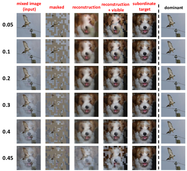
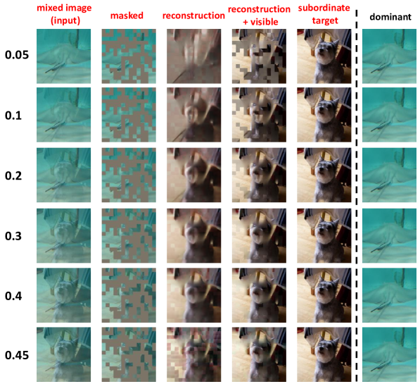
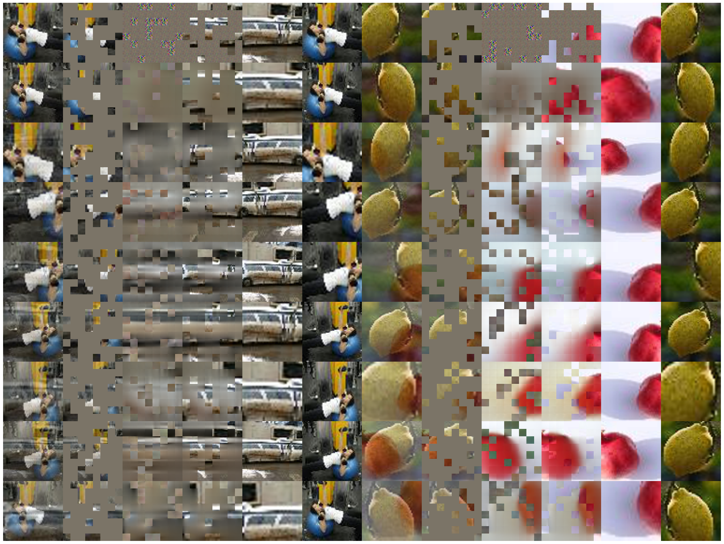
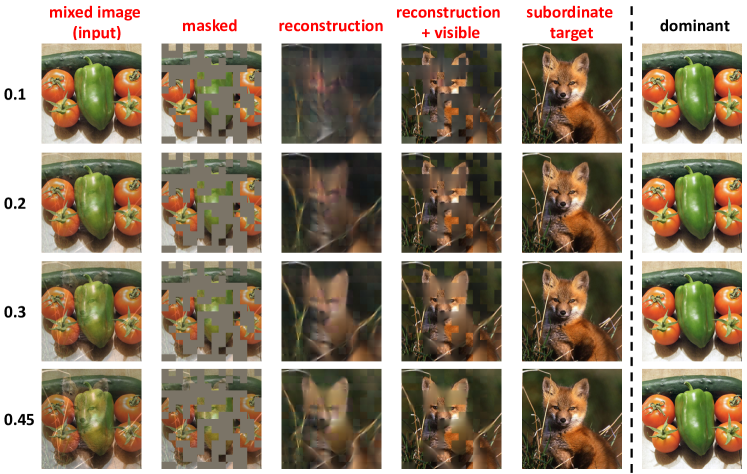
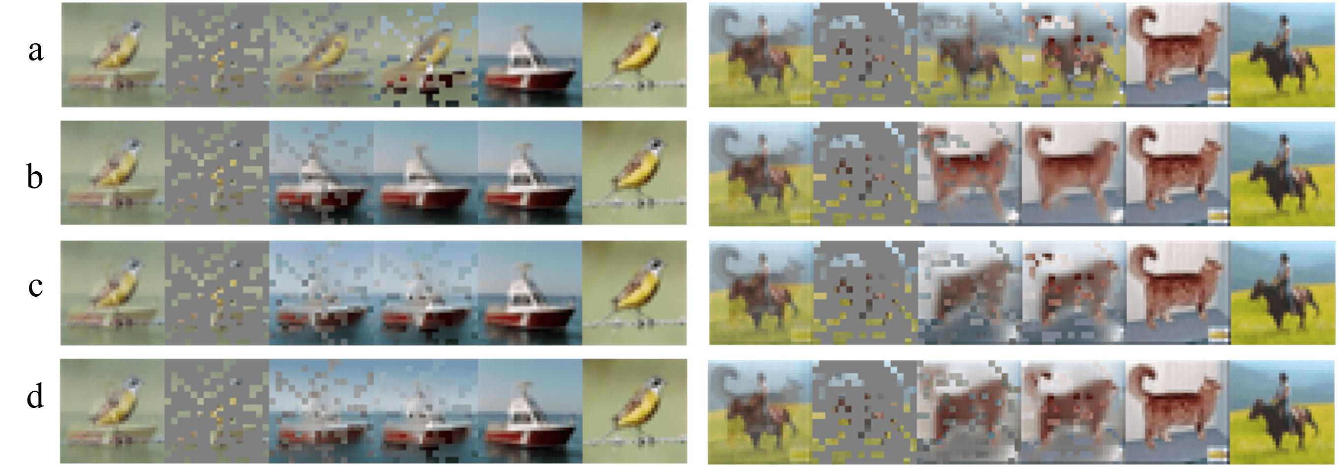
Mix Ratio. To demonstrate the separable nature of the input mixtures for subordinate reconstruction, we compared different mixture factors between 0 and 0.5, and random mixture ratios from a Beta distribution. Intuitively, lower mixing ratios contain less meaning information that the encoder may easily confuse with noise, whereas higher ratios destroy the subordinate-dominant relationship. Experimentally, we observe matching visual results shown in the Appendix (Fig. 1 and Fig. 11). The better separation performance near 0.3 indicates that i-MAE features are better dichotomized when the mix factor is balanced between noise and useful signals. Whereas below 0.15, the subordinate image is noisy and reconstructions are not interpretable, mixing ratios above 0.45 break the subordinate relationship between the two images, and the two features are harder to distinguish from each other. Moreover, Fig. 1 presents a problematic case where a mix factor of 0.45 reconstructs dominant features (hence the green patches in the background).

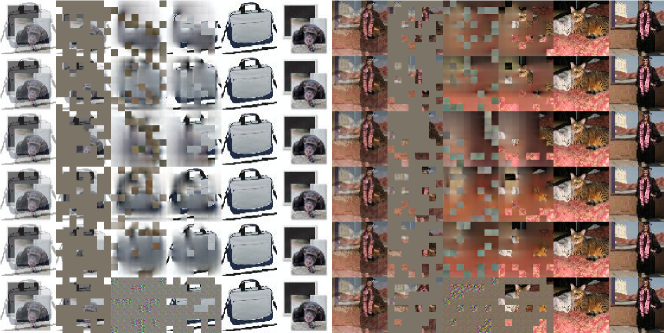
Mask Ratio. In i-MAE, visible information of the subordinate image is inherently limited by the unbalanced mix ratio, in addition to masking. Hence, a high masking ratio (75% (He et al., 2022)) may not be necessary to suppress the amount of information the encoder sees, and we consequently attempt lower ratios of 50%, 60% to introduce more information about the subordinate target. As shown in Fig. 3, a lower masking ratio of 0.5 or 0.6 can significantly improve reconstruction quality.

Combining our findings in mix and mask ratios, we empirically find that i-MAE can compensate for the information loss at low ratios with the additional alleviation of more visible patches (lower mask ratio). Illustrated in Fig. 1, we display a case of i-MAE’s reconstruction succeeding in separating the features an input with $\alpha=0.1$ mix factor and 0.5 masking ratio. Through studying the mix ratio and masking ratio, we reveal that i-MAE can learn linearly separable features under two conditions: (i) enough information about both images must be present (determined by the trade-off between mask ratio and mix ratio). (ii) the image-level distinguishing relationship between minority and majority (determined by mix ratio) is potent enough for i-MAE to encode the two images separately.

ViT Backbone Architecture. We studied whether different scales of ViT effect linear separation in the Appendix of Fig. 5. Our results show that larger backbones are not necessary for i-MAE to disentangle features on small datasets, as the insufficient training data cannot fully utilize the capability; however, large ViTs are crucial to the large-scale ImageNet-1K.

4.2.2 Ablation for Degree of Semantics

Semantic Mixes. Depending on the number of classes and their overall size, datasets in pristine states usually contain around 10% (e.g., CIFAR-10) to $<$1% (e.g. ImageNet-1K) samples pertaining to the same class, meaning that by default, uniformly random sampling mixtures will most likely be of different objects. On the other hand, the semantics-controllable mixture scheme examines whether the introduction of semantically homogeneous mixtures affects the classification performance. That is, we intentionally test to see if similar instances during pre-training negatively influence the classification performance.

As shown in Tab. 1, after i-MAE pre-training, we perform finetuning and linear probing on classification tasks to evaluate the degree of semantics learned given different amounts of intra-class mix $\bm{r}$. From Tab. 1, we discover that i-MAE overall has a stronger performance in finetuning and linear probing with a non-zero same-class ratio. Specifically, a high $\bm{r}$ of 1.0 increases the accuracy in linear evaluation most in all datasets, meaning that the quality of learned features is best and separated, and it gains a strong prior of category information for semantically enhanced mixtures. On the other hand, setting $\bm{r}=0.5$ is advantageous during finetuning, as it gains a balanced prior of separating both intra- and inter-class mixtures.

Table 1: Classification performance of models pre-trained with semantics-controllable mixture with intra-class mix rate $\bm{r}$ from 0.0 to 1.0. Whereas the lower bound represents inputs that are all mixes of different classes, $\bm{r}=1.0$ pre-trains with solely mixtures of same-labeled objects.

	CIFAR-10		CIFAR-100		Tiny-ImageNet
Same-class Ratio	Finetune	Linear	Finetune	Linear	Finetune	Linear
baseline	90.78	72.47	68.66	32.57	59.28	19.62
0.0	91.67	70.53	68.34	29.22	60.91	18.23
0.5	92.34	72.80	69.50	30.11	60.58	18.51
1.0	91.60	77.61	69.33	33.39	61.13	20.40

Figure 3: Comparisons between different mask ratios on Tiny-ImageNet validation dataset. i-MAE produces enhanced visual reconstructions from lower masking ratios when reconstructing images.

Table 2: Linear separation metric using $\ell_{2}$ distance calculated before and after linear regression on CIFAR-10, CIFAR-100, Tiny-ImageNet, and ImageNet. Reported results are from 100 samples trained for 2000 (5000 on ImageNet-1K) epochs and a fixed mix ratio of 0.3. i-MAE and i-MAE without distillation are embedding after disentanglement.

	CIFAR-10		CIFAR-100		Tiny-ImageNet		ImageNet-1K
	Before	After	Before	After	Before	After	Before	After
Baseline	3.5899	0.0584	3.0840	0.0487	10.38	0.0204	13.91	0.2004
i-MAE w/o distill	0.1384	0.0568	0.2999	0.0475	0.0723	0.0363	0.8799	0.1316
i-MAE	0.0331	0.0474	0.0312	0.0456	0.0708	0.0352	0.2760	0.1838

Figure 4: Qualitative comparisons on CIFAR-10. Row (a): baseline vanilla MAE; (b): MAE with unmixed input; (c): our i-MAE without distillation; and (d): i-MAE with distillation.

Table 3: Finetuning classification acc. on i-MAE with best semantics-controllable mixture settings.

Method	CIFAR-10	CIFAR-100	Tiny-ImageNet
Baseline	90.78	68.66	59.28
i-MAE	92.00	69.50	61.63

Table 4: Linear Evaluation accuracy of i-MAE with best semantics-controllable mixture settings.

Method	CIFAR-10	CIFAR-100	Tiny-ImageNet
Baseline	72.47	32.57	19.62
i-MAE	77.61	33.39	20.40

4.3 Results of Final Evaluation

In this section, we provide a summary of our main findings: how separable are i-MAE embedded features and the amount of semantics embedded in mixed-representations. Then, we evaluate the quality of our features with classification and analyze the features.

4.3.1 Separability

In this section, we show how i-MAE displays properties of linear separability, visually and quantitatively, and demonstrate our advantage over baseline (vanilla MAE).

In a visual comparison of the disentanglement capability in Fig. 4, vanilla MAE does not perform well out-of-the-box. In fact, the reconstructions represent the mixed input more so than the subordinate image. Since the mixture inputs of i-MAE is a linear combination of the two images, and our results show i-MAE’s powerful ability to reconstruct both images, even at very low mixture ratios, we attribute such ability to i-MAE’s disentanglement strongly correlating with the vanilla MAE’s features.

As aforementioned, we previously gave the formal definition of linear separability; now, we empirically illustrate the strength of the linear relationship between MAE’s features and i-MAE’s disentangled features with a linear regressor. We employ $\ell_{2}$ distance as our criterion and results are reported in Tab. 2. Experimentally, we feed mixed inputs to i-MAE and a singular image to the target model (vanilla MAE), Before indicates that we directly calculate the distance between the “ground-truth” features from pre-trained MAE and our disentangled features. After indicates that we train the linear regressor’s parameters to fit the “ground-truth”. Baseline is the model trained without the disentanglement module. It can be observed that our i-MAE has a significantly smaller distance than the vanilla model, reflecting that such a scheme can obtain better separability ability.

4.3.2 Semantics

Finetune and Linear Evaluation. We evaluate our i-MAE’s performance through finetuning and linear evaluation of regular inputs and targets. For all approaches in the finetuning phase, we only use Mixup as augmentation; no extra augmentations are used for the linear evaluation phase. Classification performance is outlined in Tab. 4 and Tab. 4. It can be observed that i-MAE outperforms the baseline by a remarkable margin. As our features are learned from a harder scenario, they encode more information with a more robust representation and classification accuracy. Besides, i-MAE shows a considerable performance boost with both evaluation methods.

Analysis. We emphasize that our enhanced performance comes from i-MAE’s ability to learn more separable features with the disentanglement module, and the enhanced semantics learned from training with semantics-controllable mixture. Our classification results show the cruciality of MAE learning features that are linearly separable, which can help identify between different classes. However, to correctly identify features with their corresponding classes, semantically rich features are needed, which can be enhanced by the intra-class mix sampling strategy.

5 Conclusion

It is non-trivial to understand why Masked Image Modeling (MIM) in the self-supervised scheme can learn useful representations for downstream tasks without labels. In this work, we have introduced a novel interpretable framework upon Masked Autoencoders (i-MAE) to explore two critical properties in latent features: linear separability and degree of semantics. We identified that the two specialties are the core for superior latent representations and revealed the reasons where is the good transferability of MAE from. Moreover, we proposed two metrics to evaluate these two specialties quantitatively. Extensive experiments are conducted on CIFAR-10/100, Tiny-ImageNet, and ImageNet-1K datasets to demonstrate our discoveries and observations in this work. We also provided sufficient qualitative results and analyses of different hyperparameters. We hope this work can inspire more studies on the interpretability of the MIM frameworks in the future.

Appendix

In the appendix, we display the detailed configurations of our experiments and elaborate with more examples of our main text, specifically:

• Section A “Datasets”: specifications of the datasets we used.

• Section B “Implementation Details”: implementation details and configuration settings for unsupervised pre-training and supervised classification.

• Section C “More Visualizations”: additional reconstruction examples on all datasets.

• Section D “Pseudocode”: a PyTorch-like pseudocode for our mixture and loss methods.

Appendix A Datasets

CIFAR-10/100 (Krizhevsky, 2009) Both CIFAR datasets contain 60,000 tiny colored images sized 32$\times$32. CIFAR-10 and 100 are split into 10 and 100 classes, respectively.

Tiny-ImageNet The Tiny-ImageNet is a scaled-down version of the standard ImageNet-1K consisting of 100,000 64x64 colored images, categorized into 200 classes.

ImageNet-1K (Deng et al., 2009) The ILSVRC 2012 ImageNet-1K classification dataset consists of 1.28 million training images and 50,000 validation images of 1000 classes.

Appendix B Implementation Details in self-supervised Pre-training, Finetuning, and Linear Evaluation

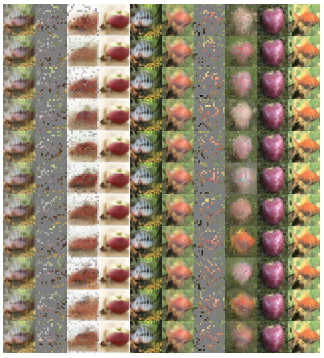
ViT architecture. In our non-ImageNet datasets, we adopt smaller ViT backbones that generally follow (Touvron et al., 2021). The central implementation of linear separation happens between the MAE encoder and decoder, with a linear projection layer for each branch of reconstruction. A shared decoder is used to reconstruct both images. A qualitative evaluation of different ViT sizes on Tiny-ImageNet is displayed in Fig. 5; the perceptive difference is not large, and generally, ViT-small/tiny are sufficient for non-ImageNet datasets.

Pre-training. The default setting for pre-training is listed in Tab. 8. On ImageNet-1K, we strictly use MAE’s specifications. For better classification performance, we use normalized pixels (He et al., 2022) and a high masking ratio (0.75); for better visual reconstructions, we use a lower masking ratio (0.5) without normalizing target pixels. In CIFAR-10/100, and Tiny-ImageNet, reconstruct ordinary pixels.

Semantics-controllable mixture. The default settings for our semantics-controllable mixtures are listed in Tab. 8. We modified the dataloader to mix, within a mini-batch, $\bm{r}$ percent of samples that have homogenous classes and $1-\bm{r}$ percent that is different.

Classification. For the classification task, we provide the detailed settings of our finetuning process in Tab. 8 and linear evaluation process in Tab. 8.

# alpha: mixture ratio

# args.beta: hyperparameter for the Beta Distribution.

#

# args.beta=1.0

for x in loader: # Minibatch x of N samples

alpha = np.random.beta(args.beta, args.beta)

sub_idx = np.argmin(alpha, 1-alpha) # Identifying the subordinate (target) image

perm = torch.randperm(batch_size) # inner-batch mix

im_1, im_2 = x, x[perm, :]

mixed_images = alpha * im_1 + (1-alpha) * im_2

#

# Subordinate Loss

loss_sub = loss_fn (model(mixed_images), im_2)

#

# update gradients

optimizer.zero_grad()

loss.backward()

optimizer.step()

...

Algorithm 1 PyTorch-style pseudocode for a single subordinate reconstruction on i-MAE.

Appendix C More Visualizations

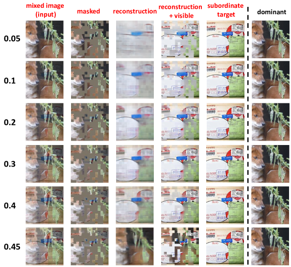
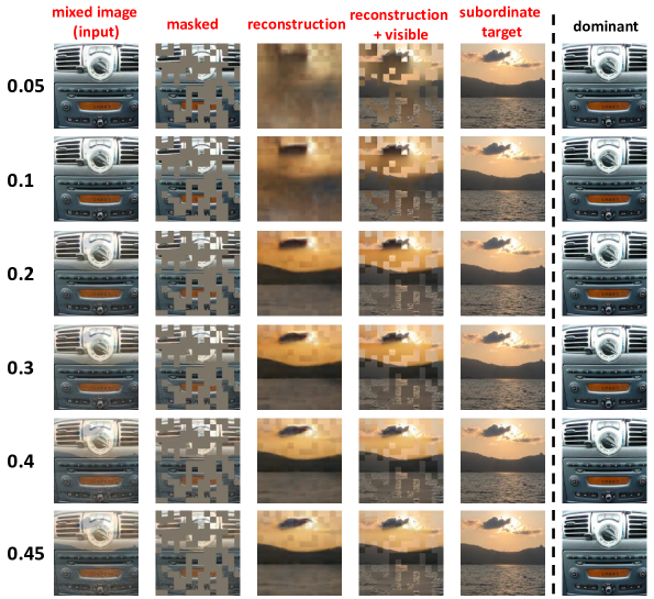
We provide extra examples of a single-branch trained i-MAE reconstructing the subordinate image. Fig. 11 are visualizations on CIFAR-100 at mix ratios from 0.1 to 0.45, in 0.05 steps. As shown in Fig. 6 and Fig. 7, we produce finer ranges of reconstructions from 0.05 to 0.45. Notice that in most cases, mixture rates above 0.4 tend to show features of the dominant image. This observation demonstrates that a low mixture rate can better embed important information separating the subordinate image.

Appendix D PyTorch Styled Pseudocode

The pseudocode of our mixture and subordinate reconstruction approach is shown in Algorithm 1. This is only a simple demonstration of our most basic framework without distillation losses. In our full-fledged i-MAE, we employ two additional distillation losses, an additional linear separation branch, and the semantics-controllable mixture scheme; nonetheless, the key implementation remains the same as the pseudocode presented here.

Figure 5: Different ViT backbones (tiny, small, and base) on Tiny-ImageNet . Reconstruction quality is moderately improved when a larger backbone is used.

Table 5: Self-supervised pre-training configurations on CIFAR-10/100, Tiny-ImageNet, ImageNet-1K. For better visualizations, we use a 0.5 mask ratio on ImageNet.

Config	CIFAR-10/100	Tiny-ImageNet	ImageNet-1K
base learning rate	1.5e-4	1.5e-4	1e-3
batch size	4,096	4,096	4,096
Mask Ratio	0.75	0.75	0.5
optimizer	AdamW	AdamW	AdamW
optimizer momentum	0.9, 0.95	0.9, 0.95	0.9, 0.95
augmentation	None	RandomResizedCrop	RandomResizedCrop

Table 6: Pre-training Configurations of with the semantics-controllable mixture scheme.

Config	CIFAR-10/100	Tiny-ImageNet
Object mix range	0.0, 0.25, 0.5, 1.0	0.0, 0.25, 0.5, 1.0
Image mix ratio	$\text{Beta}(1.0,1.0)$	$\text{Beta}(1.0,1.0)$
base learning rate	1.5e-4	3.5e-4
batch size	4,096	4,096
Mask Ratio	0.75	0.75
optimizer	AdamW	AdamW
optimizer momentum	0.9, 0.95	0.9, 0.95
augmentation	None	RandomResizedCrop

Table 7: Finetune Classification Configurations.

Config	CIFAR-10/100	Tiny-ImageNet	ImageNet-1K
Object mix range	0.0 - 1.0	0.0 - 1.0	0.0, 0.25, 0.5, 1.0
Image mix ratio	$\text{Beta}(1.0,1.0)$	$\text{Beta}(1.0,1.0)$	0.8
base learning rate	1e-3	1e-3	1e-3
batch size	128	256	1,024
epochs	100	100	25
optimizer	AdamW	AdamW	AdamW
optimizer momentum	0.9, 0.999	0.9, 0.999	0.9, 0.999
augmentation	Mixup	Mixup, RandomResizedCrop	Mixup, RandomResizedCrop

Table 8: Linear Classification Configurations.

Config	CIFAR-10/100	Tiny-ImageNet	ImageNet-1K
Object mix range	0.0 - 1.0	0.0 - 1.0	0.0, 0.25, 0.5, 1.0
Image mix ratio	0.35	0.35	0.35
base learning rate	1e-2	1e-2	1e-2
batch size	128	256	1,024
epochs	200	200	25
optimizer	SGD	SGD	SGD
optimizer momentum	0.9, 0.999	0.9, 0.999	0.9, 0.999
augmentation	None	RandomResizedCrop	RandomResizedCrop

Figure 6: More reconstructions results of i-MAE on ImageNet-1K validation images with different mixing coefficients $\bm{\alpha}$ (listed on the left) from models pre-trained with the subordinate image ${\bm{I}_{s}}$ as the only target, 0.5 mask ratio, and with distillation.

Figure 7: More reconstructions results of i-MAE on ImageNet-1K validation images with different mixing coefficients $\bm{\alpha}$ (listed on the left) from models pre-trained with the subordinate image ${\bm{I}_{s}}$ as the only target, 0.5 mask ratio, and with distillation loss.

Figure 8: Uncurated Tiny-ImageNet reconstructions of different mix ratio, from 0.05 to 0.45, subordinate images.

Figure 9: Visual reconstructions of Tiny-ImageNet validation images using semantics-controllable mixture pre-trained i-MAE.

Figure 10: CIFAR-100 subordinate reconstruction of different ratios marked on the left and right side. Similarly, reconstructions at 0.45 are confused with the dominant image.

Figure 11: Uncurated reconstructions of CIFAR-100 validation images using semantics-controllable mixture from 0.0 (topmost) to 1.0 (bottom), in 0.1 intervals.

References

- Bao et al. (2022) Hangbo Bao, Li Dong, and Furu Wei. Beit: Bert pre-training of image transformers. In ICLR, 2022.
- Chen et al. (2020) Ting Chen, Simon Kornblith, Mohammad Norouzi, and Geoffrey Hinton. A simple framework for contrastive learning of visual representations. In International conference on machine learning, pp. 1597–1607. PMLR, 2020.
- Deng et al. (2009) Jia Deng, Wei Dong, Richard Socher, Li-Jia Li, Kai Li, and Li Fei-Fei. Imagenet: A large-scale hierarchical image database. In 2009 IEEE conference on computer vision and pattern recognition, pp. 248–255. Ieee, 2009.
- Devlin et al. (2018) Jacob Devlin, Ming-Wei Chang, Kenton Lee, and Kristina N. Toutanova. Bert: Pre-training of deep bidirectional transformers for language understanding. 2018. URL https://arxiv.org/abs/1810.04805.
- Doersch et al. (2015) Carl Doersch, Abhinav Gupta, and Alexei A Efros. Unsupervised visual representation learning by context prediction. In Proceedings of the IEEE international conference on computer vision, pp. 1422–1430, 2015.
- Gidaris et al. (2018) Spyros Gidaris, Praveer Singh, and Nikos Komodakis. Unsupervised representation learning by predicting image rotations. In International Conference on Learning Representations, 2018.
- He et al. (2020) Kaiming He, Haoqi Fan, Yuxin Wu, Saining Xie, and Ross Girshick. Momentum contrast for unsupervised visual representation learning. In Proceedings of the IEEE/CVF conference on computer vision and pattern recognition, pp. 9729–9738, 2020.
- He et al. (2022) Kaiming He, Xinlei Chen, Saining Xie, Yanghao Li, Piotr Dollár, and Ross Girshick. Masked autoencoders are scalable vision learners. In Proceedings of the IEEE/CVF Conference on Computer Vision and Pattern Recognition, pp. 16000–16009, 2022.
- Henaff (2020) Olivier Henaff. Data-efficient image recognition with contrastive predictive coding. In International conference on machine learning, pp. 4182–4192. PMLR, 2020.
- Krizhevsky (2009) Alex Krizhevsky. Learning multiple layers of features from tiny images. 2009.
- Oord et al. (2018) Aaron van den Oord, Yazhe Li, and Oriol Vinyals. Representation learning with contrastive predictive coding. arXiv preprint arXiv:1807.03748, 2018.
- Radford & Narasimhan (2018) Alec Radford and Karthik Narasimhan. Improving language understanding by generative pre-training. 2018.
- Shen et al. (2022) Zhiqiang Shen, Zechun Liu, Zhuang Liu, Marios Savvides, Trevor Darrell, and Eric Xing. Un-mix: Rethinking image mixtures for unsupervised visual representation learning. In Proceedings of the AAAI Conference on Artificial Intelligence, volume 36, pp. 2216–2224, 2022.
- Touvron et al. (2021) Hugo Touvron, Matthieu Cord, Matthijs Douze, Francisco Massa, Alexandre Sablayrolles, and Herve Jegou. Training data-efficient image transformers and distillation through attention. In International Conference on Machine Learning, volume 139, pp. 10347–10357, July 2021.
- Xie et al. (2022) Zhenda Xie, Zheng Zhang, Yue Cao, Yutong Lin, Jianmin Bao, Zhuliang Yao, Qi Dai, and Han Hu. Simmim: A simple framework for masked image modeling. In Proceedings of the IEEE/CVF Conference on Computer Vision and Pattern Recognition, 2022.
- Yun et al. (2019) Sangdoo Yun, Dongyoon Han, Seong Joon Oh, Sanghyuk Chun, Junsuk Choe, and Youngjoon Yoo. Cutmix: Regularization strategy to train strong classifiers with localizable features. In Proceedings of the IEEE/CVF international conference on computer vision, pp. 6023–6032, 2019.
- Zhang et al. (2017) Hongyi Zhang, Moustapha Cisse, Yann N Dauphin, and David Lopez-Paz. mixup: Beyond empirical risk minimization. arXiv preprint arXiv:1710.09412, 2017.
- Zhang et al. (2016) Richard Zhang, Phillip Isola, and Alexei A Efros. Colorful image colorization. In European conference on computer vision, pp. 649–666. Springer, 2016.