MixMask: Revisiting Masking Strategy for Siamese ConvNets

Abstract

Recent advances in self-supervised learning have integrated Masked Image Modeling (MIM) and Siamese Networks into a unified framework that leverages the benefits of both techniques. However, several issues remain unaddressed when applying conventional erase-based masking with Siamese ConvNets. These include (I) the inability to drop uninformative masked regions in ConvNets as they process data continuously, resulting in low training efficiency compared to ViT models; and (II) the mismatch between erase-based masking and the contrastive-based objective in Siamese ConvNets, which differs from the MIM approach. In this paper, we propose a filling-based masking strategy called MixMask to prevent information incompleteness caused by the randomly erased regions in an image in the vanilla masking method. Furthermore, we introduce a flexible loss function design that considers the semantic distance change between two different mixed views to adapt the integrated architecture and prevent mismatches between the transformed input and objective in Masked Siamese ConvNets (MSCN). We conducted extensive experiments on various datasets, including CIFAR-100, Tiny-ImageNet, and ImageNet-1K. The results demonstrate that our proposed framework achieves superior accuracy on linear probing, semi-supervised, and supervised finetuning, outperforming the state-of-the-art MSCN by a significant margin. Additionally, we demonstrate the superiority of our approach in object detection and segmentation tasks. Our source code is available at https://github.com/LightnessOfBeing/MixMask.

1 Introduction

Self-supervised learning is a widely adopted paradigm to learn representations from input data without human-annotated labels. In the computer vision domain, it has shown superior performance in various tasks, such as classification, detection, and segmentation. One prevalent self-supervised learning framework is the Siamese Network with two branches. The distance between the two branches is calculated using a similarity loss [19, 9], contrastive loss [30, 21, 6], or distillation loss [5]. Recently, Masked Image Modeling (MIM)  [20, 3, 1] has emerged and proven to be an effective approach to learning useful representation. To fully leverage the advantages from both the masked design and siamese networks, Masked Siamese Network (MSN) [1] upon ViT has been proposed. Meanwhile, convolutional networks as ConvNeXt [28] and its V2 [37] achieve competitive results in both supervised and unsupervised scenarios, highlighting ConvNets’ potential. A recent work of Masked Siamese ConvNets (MSCN) [24] has extended MSN [1] to the ConvNet-based encoder. However, this approach simply employs the masking scheme from MIM [20, 3] without adapting it to the peculiarities of Siamese ConvNet. Moreover, both MSN and MSCN heavily rely on the multicrop strategy introduced in [4, 5] to improve the performance that is hindered by erasing operation. For instance, MSN generates ten additional views using focal mask on each iteration, and MSCN generates two extra views, which are computationally expensive for training.

In general, erase-based masking heavily synergizes with the image patchify mechanism in ViT [13], which produces image patches that are independently processed by the encoder. Such independent patch-wise processing of an image allows to simply drop masked patches thus decreasing the computational cost [20]. In contrast, ConvNets process data continuously, which is not rational for dropping masked patches, ultimately leading to the same computing time, yet masked patches no longer contain meaningful semantic information. However, another issue comes from the fact that multiple contrastive frameworks use embedding loss [6, 21], which is not designed to recover the erased regions but to discriminate between the inputs. Furthermore, several works [11, 7] indicate that contrastive loss tends to learn more global and coarse-grained features. Masking operation destroys such global features leading to the slower convergence of a model. This is different from vision transformer based MIM methods [20, 3] that will recover the masked regions by operating on the pixel space using reconstruction loss.

Therefore, we identify two main drawbacks of Masked Siamese ConvNets: (I) Regular erase-based masking operation disrupts the global features that are important for the contrastive objective [7, 11]. It is straightforward that vanilla masking will drop semantic information from the input data and cannot be recovered by post-processing. For instance, if we mask 25% of image areas, 25% of information will be lost during training, and it will encumber the training efficiency. Thus, a better masking strategy is necessary to encourage models to learn better representations. (II) The default “symmetric” semantic distance loss in the siamese networks that does not take into account the semantic distance change between different views of the same image after the masking operation. Clearly, when arbitrary regions of the image get erased, the global semantic meaning of the image changes as well. An original image of a dog in the center has a substantially different meaning compared to the same image, where regions containing different body parts of a dog are masked and no longer visible. Such symmetric loss design brings relatively low influence when both of the branches are masked. However, it causes a negative effect inevitably when only one branch is masked in the architecture. Since asymmetric siamese networks [34] have been observed to be more effective to learn, a more flexible loss design with soft distance is crucial to reflect the true semantic distance between the two asymmetric branches in masked siamese convnets.

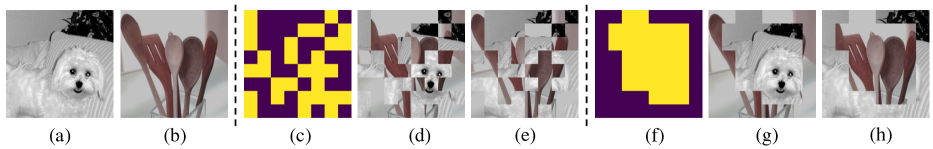
Figure 1: Illustration of the different mask patterns with a mask grid size of 8. (a) and (b) are input images. (c) is the discrete/random mask pattern, and (d) and (e) are mixed images using this mask. (f) is the blocked mask pattern, and (g) and (h) are mixed images with a blocked mask. Discrete masking breaks (c) – (e) the completeness of an object which is important for the contrastive loss because it operates on the global object level. On the other hand, blocked masking (f) – (h) preserves important global features leading to superior performance.

To address these two drawbacks, in this work, we propose to use a filling-based masking strategy to avoid information loss from erasing operation. Specifically, instead of erasing random areas in an image, we will randomly select another image and use its pixel values to fill the masked areas. Furthermore, instead of using discrete random masking that is applied in [20], we found using block-wise masking will give better performance since it can better preserve global information important for contrastive loss. Together with our mask-filling strategy block-wise masking fills the uninformative erased regions with global views from other images in a batch. To reflect the semantic distance change after the filling operation we incorporate the asymmetric loss design introduced in [34]. Compared to the erase-based strategy of MSCN, the filling-based masking method replaces uninformative erased regions with regions providing more meaningful semantic information of the input space, it does not require multicrops and only needs one additional view per image, which is more efficient than MSN and MSCN using ten and two cropping pairs. Such information from filling-based masking can be exploited by siamese networks to enhance the representation during training. Our ablation experiments show that this is a better masking solution for the Masked Siamese ConvNets.

We conducted comprehensive experiments on CIFAR-100, Tiny-ImageNet, and ImageNet-1K datasets to evaluate our proposed method. We integrated our approach into multiple Siamese ConvNets, including MoCo, BYOL, SimCLR, and SimSiam. Our method significantly improves various baseline models across all datasets. Additionally, we evaluated our learned models on the semi-supervised and supervised finetuning, as well as downstream tasks such as object detection and segmentation, and consistently observed improvements.

Our contributions in this work are as follows:

• We reveal that Siamese ConvNets exhibit lower convergence using the traditional erase-based masking scheme. To this end, we propose a simple yet effective filling-based masking strategy that is more aligned with the image-level contrastive objective for self-supervised Siamese ConvNets.

• We show that block-wise masking provides superior performance on Masked Siamese ConvNets to the discrete random masking, commonly used in self-supervised representation learning frameworks [20, 24, 1]. This observation highlights the difference of our method from MSCN [24] and Un-Mix [34].

• We integrate a flexible loss design with soft distance to adapt the integrated masking and siamese architecture, as well as to avoid mismatches between transformed input and objective in Masked Siamese ConvNets.

• Extensive experiments are performed on various datasets and siamese frameworks to demonstrate the effectiveness and generality of the proposed method. We verify that our approach is consistently superior to MSCN on linear probing, semi-supervised fine-tuning, detection and segmentation downstream tasks.

2 Related Work

Masked Image Modeling. Masked Image Modeling aims at learning informative representations by reconstructing a masked image to its original view. He et al. [20] proposed a simple transformer-based Masked Autoencoder (MAE) architecture that employs Mean Squared Error (MSE) loss to reconstruct the original image. BEiT [3] introduced self-supervised pretraining by tokenizing the input image into visual tokens and applying masking. Spatiotemporal representation learning using MAE was proposed in [15] by Feichtenhofer et al. Several works [18, 2, 16] have explored ways to adapt MAEs to handle multimodal data.

Masked Siamese Networks. Recent developments in masked image modeling and siamese self-supervised learning have prompted research efforts to combine these two techniques. One such approach, Masked Siamese Networks (MSN), was proposed in [1]. MSN generates an anchor view and a target view and applies masking operations exclusively to the anchor branch. To assign masked anchor representations to the same cluster as the unmasked target, the method employs prototype cluster assignment. By contrast, CNNs are less compatible with masked images as they operate at the pixel level, which can cause image continuity to be disrupted by masking operations. To address this issue, Masked Siamese ConvNets (MSCN) were introduced in [24]. This study investigates and provides guidelines for adapting CNN-based siamese self-supervised learning frameworks to be compatible with masking operations.

Mixture-based Data Augmentations. Several mixture-based techniques have been demonstrated to be effective data augmentation methods in the computer vision domain. Typically, these methods combine two images to generate a new image, referred to as their mixture, and modify the loss function to reflect the semantic distance changes in the resulting mixture image. Initially, Mixup [42] and Manifold Mixup [35] were introduced for supervised learning, whereby pairs of images in the same batch are mixed at a global pixel level using a soft coefficient $\lambda$. Subsequently, local region-based techniques such as CutMix [40] and an attentive scheme [36] were proposed using the same loss design as Mixup. Finally, Un-Mix [34] demonstrates how to integrate Mixup and CutMix for self-supervised learning.

Self-supervised Learning. Self-supervised learning (SSL) is a prevalent technique for representation learning that leverages vast amounts of unlabeled data. Early SSL approaches in the field of computer vision were based on pre-text tasks [29, 17, 33, 43]. A pivotal advancement in SSL was the introduction of a simple contrastive learning framework by [10, 6], which utilized a siamese architecture in conjunction with an InfoNCE [30] contrastive loss. MoCo [21] implemented a memory bank to store negative samples, but several studies have shown that negative pairs are not always necessary. BYOL [32] employed an asymmetric architecture with EMA, where the online network attempts to predict the representations of the target network. SimSiam [9] provided a straightforward siamese framework that incorporated a stop-gradient operation on one branch and an additional predictor step on the other. More recently, SSL has begun to adopt the use of vision transformers [13]. DINO [5] combined a distillation loss with vision transformers in a siamese framework.

3 Approach

In this section, we first introduce each component of our framework elaborately, including: (i) a filling-based masking strategy; (ii) an asymmetric loss formulation with soft distance to match the proposed mix-masking scheme; (iii) permutation strategies if incorporating with other mixing approaches. Then, we provide an overview of the proposed architecture comparing to the basic model. Finally, we discuss in detail the design principles, insights, and differences from other counterparts.

3.1 Perspective on Masking Strategy

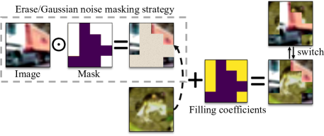
Figure 2: Illustration of the proposed filling-based masking strategy. The gray dashed box shows Erase/Gaussian noise [24] masking strategy. A formal definition of a switch image in the case of reverse permutation is given in Equation 2.

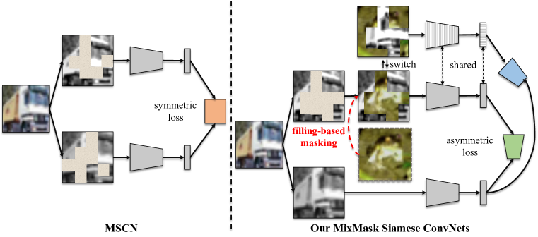
Figure 3: Illustration of the Masked Siamese ConvNets (left) and our proposed framework (right). MixMask branch incorporates asymmetry into the loss function design by generating images with different rates of similarity to the images in the original branch. In MixMask branch image of the truck is presented twice with different levels of similarity to the image in the original branch due to the regions masked with contents of another image.

Masking Scheme: Erasing or Filling? In Fig. 2, the Erase/Gaussian noise masking strategy is illustrated inside the dashed box. In such strategy, erased regions can be filled with a Gaussian noise [24]. Different from Masked Image Modeling (MIM), which is to reconstruct the masked contents for learning good representation, the Masked Siamese Networks will not predict the information in removed areas, so erasing will only lose information and is not desired in the learning procedure. In contrast to erase-based masking, our filling-based strategy will repatch the removed areas using an auxiliary image, as shown in the right part of Fig. 2. After that, we will switch the content between the main and auxiliary images to generate a new image for information completeness of the two input images. For a given original image $\bm{I}_{i}$ we define its mixture as a mix of the pair $(\bm{I}_{i},\bm{I}_{n-i})$ and switch image of $\bm{I}_{i}$ as a mixture of the pair $(\bm{I}_{n-i},\bm{I}_{i})$. Although the mixture contains information from another image, which may have different semantics, it will still be beneficial by cooperating with the soft loss design, discussed in Section 3.2, which takes into account the degree of each individual image included in the mixture.

Masking Pattern: Blocked or Discrete? Masking pattern determines the difficulty for the model to generate representations in siamese networks, even if the masking ratio is the same, the representation will still be different for different masking patterns. It will directly influence the information of input to further affect the latent representations. Our observation on Masked Siamese ConvNets is opposite to that in MIM methods, which found discrete/random masking is better [20, 39]. From our empirical experiments, on CIFAR-100, blocked and discrete masking patterns achieve similar accuracy and discrete is slightly better, however, on Tiny-ImageNet and ImageNet-1K, blocked mask clearly shows superiority over discrete/random. We explain this as that if the input size is small, the mask pattern is not so necessary since the semantic information of the object is still preserved. On larger datasets like Tiny-ImageNet and ImageNet-1K, discrete/random masking will entirely destroy the completeness of the object in an image, as shown in Fig. 1 (d, e), while this is crucial for ConvNet to extract a meaningful representation of the object. Blocked masking also better synergizes with the contrastive objective, which is biased to learn global features [7, 11]. Therefore, blocked masking shows superior ability on the MSCN and is a better choice than random discrete masking.

3.2 Perspective on Distance in Siamese Networks

Objective Calculation: Inflexible or Soft? It has been observed [34] that different pretext and data processes (e.g., masking, mixture) will change the semantic distance of two branches in the siamese networks, hence the default symmetric loss will no longer be aligned to reflect the true similarity of the latent representations. It thus far has not attracted enough attention for such a problem in this area. In this work, we introduce a soft objective calculation method that can fit the filling-based masking strategy in a better way. To calculate the soft distance, firstly, we start by generating a binary mask with a fixed grid size that will later be used to mix a batch of images, denoted as $\bm{I}$, from a single branch. In case when we use a reverse permutation to obtain the mixture, each image in the batch with index $i$ is mixed according to the mask with the image in the same batch but with index $n-i$ as described in Equation 1:

$$\text{mix}_{i} =\text{mix}(\bm{I}_{i},\bm{I}_{n-i})=m\odot\bm{I}_{i}+(1-m)\odot\bm{I}_{n-i}$$ (1)

$$\text{switch}_{i} =\text{mix}(\bm{I}_{n-i},\bm{I}_{i})=m\odot\bm{I}_{n-i}+(1-m)\odot\bm{I}_{i},$$ (2)

where $\bm{n}$ is batch size and $m$ is mask. The mixed image contains parts from both $\bm{I}_{i}$ and $\bm{I}_{n-i}$ whose spatial locations in the mixture are defined by the contents of the binary mask. Using $m$ and $1-m$ ensures that each region in the mixture will contain pixels from exactly one image and that there will be no empty unfilled regions. Furthermore, to reflect the contribution of each image in the mixture, we calculate a mixture coefficient $\lambda$, which is equal to the ratio of the masked area to the total area of the image using the Equation 3:

$$\lambda=\frac{\sum\limits_{x,y}\mathbbm{1}[mask(x,y)=1]}{{width}\cdot{height}},$$ (3)

where $\mathbbm{1}$ is the indicator function that measures the masked area of an image.
Loss Function. The final loss is defined as a summation of the original loss and mixture loss:

$$\mathbbm{L}=\mathbbm{L}_{\text{Orig}}+\mathbbm{L}_{\text{MixMask}}.$$ (4)

Here we take a contrastive loss from MoCo [21] as an example, where $q$ and $k$ are two randomly augmented non-mixed views of the input batch. The notation stems from queries and keys from MoCo nomenclature, the $\mathbbm{L}_{\text{Orig}}$ will be:

$$\begin{split}\mathbbm{L}_{\text{Orig}}=&-\log\frac{\exp\left(q\cdot k/\tau\right)}{\sum_{i=0}^{K}\exp\left(q\cdot k_{i}/\tau\right)}.\end{split}$$ (5)

The mixture term $\mathbbm{L}_{\text{MixMask}}$ will contain two terms which are scaled with $\lambda$ coefficient:

$$\mathbbm{L}_{\text{MixMask}} =\lambda\cdot\mathbbm{L_{\uparrow}}+(1-\lambda)\cdot\mathbbm{L_{\downarrow}}=$$ (6)

$$=-(\lambda\cdot\log\frac{\exp\left(q_{\uparrow}\cdot k/\tau\right)}{\sum_{i=0}^{K}\exp\left(q_{{\uparrow}}\cdot k_{i}/\tau\right)}+$$

$$(1-\lambda)\cdot\log\frac{\exp\left(q_{\downarrow}\cdot k/\tau\right)}{\sum_{i=0}^{K}\exp\left(q_{{\downarrow}}\cdot k_{i}/\tau\right)}),$$

where $q_{\uparrow}$ and $q_{\downarrow}$ are normal and reverse orders of mixed queries in a mini-batch respectively, $k$ is the unmixed single key, $\lambda$ is calculated according to the Equation 3 and $\tau$ is the temperature.

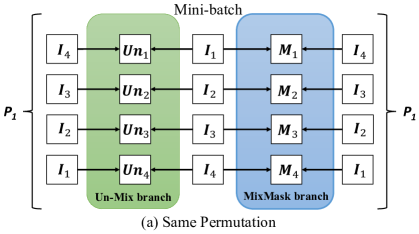
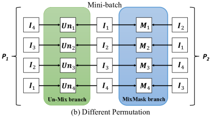
Figure 4: Illustration of different permutation strategies when Un-Mix and MixMask are used together. $I_{i}$ denotes an image in mini-batch, $Un_{i}$ denotes a mixture image obtained using Un-Mix, and $M_{i}$ denotes a mixture image generated using MixMask. In (a), we use the same reverse permutation $P_{1}$ for both the Un-Mix branch and the MixMask branch, and thus we mix the same pair of images twice. In (b), we use two different permutations $P_{1}$ (reverse) and $P_{2}$ (different random permutation) therefore, different pairs of images are mixed in different branches yielding a more diverse set of training data.

Permutation Strategies: Same or Shuffled? We offer insights on how our method can be integrated with Un-Mix [34]. Specifically, we investigate how different permutation strategies used to produce an image mixture impact the final performance of the model trained with both Un-Mix and MixMask to further enhance the performance. Recall that, by default, Un-Mix employs a reverse permutation to generate the image mixture, i.e., the image with index $i$ is mixed with the image with index $n-i$. Through empirical analysis, we demonstrate that to achieve optimal model performance when trained with both Un-Mix and MixMask, we need to use a distinct permutation in the MixMask branch. This approach allows for a more diverse set of mixed images, as different image pairs are mixed in the Un-Mix and MixMask branches, respectively. This permutation strategy ultimately enhances the model’s generalization ability. A detailed explanation of the strategy is presented in Fig. 4.

3.3 Framework Overview

Our framework overview is shown in Fig. 3. In this figure, the left is the conventional Masked Siamese ConvNets (MSCN), right is our proposed MixMask with asymmetric distance loss. The motivation behind this design is that directly erasing regions will lose a significant proportion of information in the Siamese ConvNets, which cannot be recovered by post-training. This is quite different from the mechanism of Masked Autoencoders (MAE) [20] that predict masked areas to learn good representations. According to this, we propose a filling-based scheme to overcome the drawback. The soft distance loss is designed to fit the true similarity of the two branches. Despite its conceptual simplicity, we empirically show that with the integrality of mix-masking and objective, we can learn more robust and generalized representations from the masked input.

3.4 Discussions

Symmetric or Asymmetric losses in Siamese ConvNets? Siamese networks can be categorized into several paradigms based on the input and objective spaces: (i) Input symmetric + objective symmetric (regular siamese models). (ii) Input asymmetric + objective asymmetric (Un-Mix [34]). (iii) Input asymmetric (slightly) + objective symmetric (MSCN [24]). Here, input symmetric denotes the use of the same probability of data augmentations to generate two different views of samples from the same image. Input asymmetric refers to one view/branch containing additional data augmentations, such as Mixup or CutMix. Objective symmetric implies the utilization of regular contrastive loss or similarity loss, whereas objective asymmetric indicates that the similarity is calibrated by a soft coefficient. In general, both input and objective are asymmetric, enabling the model to learn finer and more nuanced information, resulting in a more robust representation for downstream tasks.

Relationship to Counterparts. MSN and MSCN utilize regular erase-based masking and Un-Mix approach integrates Mixup and CutMix techniques into siamese networks for self-supervised learning. In contrast, our MixMask method is a generalized masking approach specifically designed for siamese networks that allows for arbitrary mask area shapes. Our empirical study demonstrates that MixMask exhibits strong representation learning capabilities. Interestingly, MixMask is also compatible with Un-Mix and can be employed jointly to further improve performance and achieve state-of-the-art accuracy.

4 Experiments

Base Models. In our experimental section, we use base models including: MoCo V1&V2 [21, 8], Un-Mix [34], SimCLR [6], BYOL [32] and SimSiam [9]. A detailed introduction for each of them is in supplementary material.

Datasets and Training Settings. We conduct experiments on CIFAR-100 [25], Tiny-ImageNet [26] and ImageNet-1K [12] datasets. For CIFAR-100 and Tiny-ImageNet, we train each framework for 1000 epochs with ResNet-18 [23] backbone. For ImageNet-1K, we pretrain ResNet-50 for 200 and 800 epochs and then finetune a linear classifier on top of the frozen features for 100 epochs and report Top-1 accuracy. We use MoCo (and MoCo V2 for ImageNet-1K) as a base framework unless stated otherwise. We report Top-1 on linear evaluation, except the case of MoCo on CIFAR-100 and Tiny-ImageNet for which we provide k-NN accuracy. ^∗ indicates that we build our method upon Un-Mix. We provide full training configurations in the supplementary material.

4.1 Ablation Study

In the experiments, we use a blocked masking strategy, masking ratio of 0.5, and grid size of 2, 4, 8 for CIFAR-100, Tiny-ImageNet, and ImageNet-1K if not stated otherwise.

Masking Strategy. We first explore how different masking strategies affect the final result. We consider three different hyperparameters: grid size, grid strategy, and masking ratio. To make our experiments more reliable, we consider three datasets with different image sizes: CIFAR-100: 32$\times$32, Tiny-ImageNet: 64$\times$64, and ImageNet-1K: 224$\times$224.

The first parameter grid size specifies the granularity of the $n\times n$ square grid of the image. We consider the following values of $n=2,4,8,16,32,48$. However, we have different upper bounds for different datasets depending on the spatial size of the images. From our experiments, we can conclude that a very large grid size completely disrupts the semantic features of the image and leads to poor performance. Our results indicate that optimal grid size increases proportionally to the input size of the image. We obtain the optimal grid size for CIFAR-100 is 2, for Tiny-ImageNet is 4, and for ImageNet-1K is 8. The masks with very small and very large grid sizes show bad performance. We think this happens because a small grid size does not provide enough variance in the mask structure whilst a large grid size destroys the important semantic features of the image.

We consider two different strategies for the random mask generation, namely discrete/random mask and blocked mask. We generate a blocked mask according to the algorithm described in [3]. A discrete mask does not have any underlying structure, whilst a blocked mask is generated in a way to preserve global spatial continuity and, thus, is more suitable for capturing global semantic features. For CIFAR-100, we observe a negligible difference between blocked and discrete masks. On the other hand, for Tiny-ImageNet and ImageNet-1K, which have larger spatial sizes of the image, blocked mask performs better than discrete. This observation is different from MIM-based approaches [20, 39], where a discrete mask achieves better performance and highlights the importance of maintaining global features when generating an image mixture as opposed to the case when erasing parts of the image by performing a vanilla masking operation. This also reflects the different mechanisms and requirements of reconstruction-based and siamese-based self-supervised learning approaches.

Table 1: Ablation study on masking and switch strategies using MoCo V1/V2 on various datasets with original and MixMask branches. k-NN accuracy averaged over 3 runs is reported.

	CIFAR-100	Tiny-ImageNet	ImageNet-1K
Input size	32$\times$32	64$\times$64	224$\times$224
Grid Size
2$\times$2	baselinecolor68.1	46.4	68.4
4$\times$4	67.6	baselinecolor47.4	69.0
8$\times$8	67.5	46.5	baselinecolor69.2
16$\times$16	–	46.1	68.5
32$\times$32	–	–	68.7
48$\times$48	–	–	68.8
Masking Strategy
blocked	67.8	baselinecolor47.4	baselinecolor69.2
discrete	baselinecolor68.1	46.4	68.4
Masking Ratio
0.25$|$0.75	66.8	45.6	68.5
0.5	baselinecolor68.1	baselinecolor47.4	baselinecolor69.2
uniform(0, 1)	67.6	45.5	68.7
uniform(0.25, 0.75)	67.8	47.0	68.9
Switch Mixture
Yes	baselinecolor68.1	baselinecolor47.4	baselinecolor69.2
No	67.3	45.6	67.8

For the masking ratio, we consider two cases with constant values of $0.5$ and $0.25/0.75$ (as there is no difference between these two due to the loss function design) and two cases when the value is sampled from the uniform distribution with different bounds. We obtain the best results for masking ratio $0.5$ under different settings, conjecturing that this value causes the blocked mask to generate consistent global views for both of the images being mixed. Sampling masking ratio from a uniform distribution with bounds $0.25$ and $0.75$ yields better results than using $0$ and $1$ as bounds. We believe this shows that extreme values of masking ratio close to either $0$ or $1$ generate a mixture where one image heavily dominates over the other when in the optimal mixture, areas of each image should be roughly proportional.

Switch Mixture. We also examine the efficacy of the second term in the mixture loss in Equation 6, which is computed using switch images and multiplied with soft coefficient $(1-\lambda)$. Certainly, having two terms in the mixture loss part is beneficial and gives better results in Table 1 on all datasets as it provides more training signal.

Training Budgets. We test our method with different training budgets, including 200, 400, 600, 800, and 1000 epochs on CIFAR-100 using MoCo, SimCLR, and SimSiam. The results are shown in Fig. 5. We can observe our method achieves consistent improvement over various frameworks. We also provide training loss and accuracy curves for 1000 epoch training configuration in the supplementary material.

Figure 5: Results with different training budgets and base frameworks on CIFAR-100. MixMask consistently performs better than the baseline for every configuration. For MoCo, we report k-NN accuracy, for SimCLR and SimSiam, we report Top-1 accuracy. In these experiments, we use a grid size equal to 2 for MixMask. We note that for a large training budget, such as 800 or 1000 epochs, grid size 4 can sometimes provide better results due to the increased variance in the mask pattern.

Compatibility with Other Methods. We examine whether our method can be applied together with other methods like Un-Mix in the same framework. We consider two cases which are illustrated in Fig. 4: in the first case, both Un-Mix and MixMask branches use the same permutation to generate the mixed images. In the second case, mixtures for Un-Mix and MixMask are generated using different permutations. Our results in Table 2 highlight the importance of using different permutations when mixing images on Un-Mix and MixMask branches, respectively. Clearly, when using the same permutations, even though Un-Mix and MixMask perform different operations on images, there is still some redundancy and duplicated information in the produced mixtures, as each pair of images is being mixed twice (Fig. 4 (a)). On the contrary, when different permutations are used, different sets of pairs are generated in different branches (Fig. 4 (b)). Thus, we produce a more diverse and richer set of mixed training samples yielding better performance. The pseudocode is provided for the case of using both types of image mixtures in the supplementary material.

Table 2: Results using different permutation strategies when Un-Mix and MixMask are applied together. We compare two different strategies: using the same or different permutations on Un-Mix and MixMask branches. Applying different permutations produces the best performance.

	CIFAR-100			Tiny-ImageNet
Permutations	MoCo	BYOL	SimCLR	MoCo	BYOL	SimCLR
Same	69.2	71.8	baselinecolor70.1	47.4	50.8	49.7
Different	baselinecolor70.0	baselinecolor72.1	70.0	baselinecolor47.9	baselinecolor53.7	baselinecolor50.7

Furthermore, we investigate the impact of utilizing two branches concurrently on the parameter of the probability of global mixture in Un-Mix. In [34], it has been demonstrated that the optimal parameter for the global mixture (Mixup) on the ImageNet-1K dataset is $P=0$ (local mixture only). However, we question this assumption in the context of two mixture branches, as we observe that adding the MixMask branch can alter the optimal value of $P$ in Un-Mix. Through empirical analysis, we find that the best performance is achieved for $P=0.5$, as shown in Table 4. We theorize that CutMix is essentially a special case of MixMask that applies a blocked mask, thereby enabling the model to benefit from the Mixup aspect of Un-Mix.

Table 3: Results on ImageNet-1K for the optimal value of probability for the global mixture ($P$) for Un-Mix when it is used together with MixMask. We report Top-1 accuracy for the linear evaluation protocol for 100 epochs.

$P=0$	$P=0.5$	$P=1.0$
69.1	baselinecolor69.5	68.7

Table 4: Comparison of MSCN with MixMask on ImageNet-1K using MoCo V2 framework. MixMask shows better performance.

Method	Pretrain Epochs	Top-1	Pretrain Epochs	Top-1
Vanilla MoCo V2	200	67.5	800	71.1
MSCN	200	68.2	800	71.5
MixMask	200	baselinecolor69.2	800	baselinecolor71.7

Table 5: Ablation on different base framework approaches. On CIFAR-100 we use grid size 2 for MoCo and grid size 4 for all other frameworks. * indicates we build our method upon Un-Mix.

	CIFAR-100				Tiny-INet		INet-1K
	MoCo	SimSiam	BYOL	SimCLR	MoCo	BYOL	MoCoV2
Vanilla	65.7	66.7	66.8	67.1	42.8	51.4	67.5
Un-Mix [34]	68.6	70.0	70.0	69.8	45.3	52.9	68.5
MixMask	68.4	69.8	71.9	69.2	47.4	50.8	69.2
MixMask∗	baselinecolor70.0	baselinecolor70.6	baselinecolor72.1	baselinecolor70.0	baselinecolor47.9	baselinecolor53.7	baselinecolor69.5

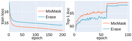
Figure 6: Comparison of training loss (left) and Top-1 accuracy (right) curves for MSCN (erase-based) and MixMask on ImageNet-1K for 200 pretraining budget. Our method outperforms MSCN by about 1%.

Table 6: Results of semi-supervised and supervised finetuning on ImageNet-1K with 1%, 10%, 100% labels. The models are pretrained with 800 epochs.

Method	1%	10%	100%
	Top-1 Acc	Top-1 Acc	Top-1 Acc
MoCo V2 [8]	50.3	66.8	76.7
SwAV [4]	53.9	70.2	–
Barlow Twins [41]	55.0	69.7	–
MSCN [24]	54.0	-	–
MixMask	baselinecolor54.5	baselinecolor69.3	baselinecolor77.7

Table 7: Object detection and segmentation results on the COCO dataset with 1x schedule and detection results on the Pascal VOC dataset. MixMask performs better than all other models on all metrics. The models are pretrained with 800 epochs.

	MS COCO 2017						Pascal VOC 2007
Method	Object detection			Segmentation			Object detection
	AP	AP50	AP75	AP	AP50	AP75	AP	AP50	AP75
MoCo V2 [8]	39.3	58.9	42.5	34.4	55.8	36.5	57.4	82.5	64.0
SwAV [4]	38.4	58.6	41.3	33.8	55.2	35.9	56.1	82.6	62.7
Barlow Twins [41]	39.2	59.0	42.5	34.3	56.0	36.5	56.8	82.6	63.4
MSCN [24]	39.1	59.1	42.1	34.2	55.7	36.4	57.5	83.0	64.4
MixMask	baselinecolor39.8	baselinecolor60.0	baselinecolor43.0	baselinecolor34.8	baselinecolor56.3	baselinecolor37.0	baselinecolor57.9	baselinecolor83.0	baselinecolor64.5

Results for Different Base Frameworks. In Table 5 we consider the generalizability of our method by applying it on top of four different self-supervised learning frameworks. When applying our method upon Un-Mix, we yield superior performance in all cases. Plain MixMask also provides a competitive performance in all the experiments.

4.2 Comparison and Superiority to MSCN

We present evidence demonstrating that our proposed approach, MixMask, outperforms MSCN [24]. Specifically, Table 4 shows the results of linear probing for both training budgets of 200 and 800 epochs. MixMask achieves superior performance by proposing a method to fill the erased regions with meaningful semantics. Additionally, we evaluate MixMask and MSCN on various downstream tasks, including semi-supervised and supervised fine-tuning (Table 7) and object detection and segmentation (Table 7). The results demonstrate that MixMask outperforms MSCN and even surpasses the performance of SwAV in semi-supervised fine-tuning. Moreover, MixMask achieves better results than MSCN on all evaluation metrics for detection and segmentation. Notably, our approach is conceptually simpler and computationally more efficient than MSCN, which requires combining multiple masking strategies, including Random, Focal, Channel-Wise masks, adding Gaussian noise, and multicrops.

4.3 Comparison to State-of-the-art Approaches

We provide a comparison with state-of-the-art approaches in Table 5. For CIFAR-100 and Tiny-ImageNet we report k-NN accuracy obtained from our experiments. For ImageNet-1K we report Top-1 accuracy either from our experiments or from other papers. When reporting values for Un-Mix and MixMask, we use MoCo as an underlying framework. MixMask shows competitive results across all the datasets. As indicated in Table 5, it is able to generalize well across different self-supervised learning frameworks.

4.4 Results on Semi and Supervised Finetuning

For the semi-supervised and supervised finetuning on ImageNet-1K, we follow the protocol described in [24]. We explore three different data regimes of 1%, 10%, and 100% of labels and finetune all models for 20 epochs. We use lr = 0.002/0.001/0.001 on stem and lr = 0.5 on the classification layer for 1% / 10% / 100% labels, respectively. The results are given in Table 7, MixMask outperforms MSCN as well as MoCoV2 and SwAV on 1% data regime and shows competitive performance to SwAV and Barlow Twins on 10%.

4.5 Results on Object Detection and Segmentation

We test our method on the downstream task of object detection and segmentation. For that, we finetune a Faster-RCNN [31], and Mask-RCNN [22] models implemented in Detectron2 [38] on Pascal VOC 2007 [14], and MS COCO 2017 [27] datasets. For VOC 2007, we follow the standard evaluation protocol in [21] with 24k training iterations. For COCO, we use $1\times$ schedule configuration from [38]. The results in Table 7 verify the superiority of the proposed MixMask to all other frameworks, including MSCN.

5 Conclusion

In this work, we have proposed a new approach of MixMask, which combines a dynamic and asymmetric loss design together with a mask-filling strategy for the Masked Siamese ConvNets. We have shown that our asymmetric loss function performs better than the standard symmetric loss used in MSCN. Furthermore, we have solved the problem of learning efficiency in vanilla erase-based masking operation by employing a filling-based masking strategy, where another image is used to fill the erased regions. In addition, we have provided a recipe for integrating MixMask with other mixture methods and explained the effect of the different masking parameters on the quality of the learned representations. Extensive experiments are conducted on CIFAR-100, Tiny-ImageNet, and ImageNet-1K across different frameworks and downstream tasks. Our method outperforms the state-of-the-art MSCN baseline on linear probing and several downstream tasks.

Supplementary material

Appendix A Base Models & Datasets

In this section, we provide a description of self-supervised learning frameworks and datasets that we used in the experiments. To test our method, we tried to select a diverse set of frameworks that incorporate different mechanisms to avoid model collapse and follow different design paradigms, i.e., vanilla contrastive learning with negative pairs vs knowledge distillation.

A.1 Base Models

MoCo V1&V2 [21, 8] is a self-supervised contrastive learning framework that employs a memory bank to store negative samples. MoCo V2 is an extension of the original MoCo, which introduces a projection head and stronger data augmentations.

Un-Mix [34] is an image mixture technique with state-of-the-art performance for unsupervised learning, which uses CutMix and Mixup at its core. It smooths decision boundary and reduces overconfidence in model predictions by introducing an additional mixture term to the original loss value, which is proportional to the degree of the mixture.

SimCLR [6] is a siamese framework with two branches that uses contrastive loss to attract positive and repel negative instances using various data augmentations.

BYOL [32] is a self-supervised learning technique that does not use negative pairs. It is composed of two networks, an online and a target. The task of an online network is to predict the representations produced by the target network. EMA from the online network is used to update the weights of the target.

SimSiam [9] The authors examined the effect of the different techniques which are commonly used to design siamese frameworks for representation learning. As a result, they proposed a simple framework with two branches that relies on the stop gradient operation on one branch and an extra prediction module on the other.

A.2 Datasets

CIFAR-100 [25] consists of 32$\times$32 images with 100 classes. There are 50,000 train images and 10,000 test images, 500 and 100 per class, respectively.

Tiny-ImageNet [26] is a dataset containing 64 $\times$ 64 colored natural images with 200 classes. The test set is composed of 10,000 test images, whilst the train contains 500 images per category, totaling 100,000 images.

ImageNet-1K [12] has images with a spatial size of 224$\times$224. 1,281,167 images span the training set, which includes 1K different classes, whilst the validation set includes 50K images.

Appendix B Training Configurations

In this section we provide hyperparameter settings for:

• Training on CIFAR-100 and Tiny-ImageNet in Table 8.

• Pretraining and linear probing on ImageNet-1K configurations are shown in Table 10.

• Configurations for semi-supervised and supervised fine-tuning on ImageNet-1K are given in Table 10.

• For object detection and segmentation we use the Detectron2[38] library and follow the $1\times$ recipe on COCO and standard 24k training protocol on Pascal VOC07.

Table 8: Training settings on CIFAR-100 and Tiny-ImageNet. Slash separated values correspond to CIFAR-100 and Tiny-ImageNet, respectively.

MoCo		SimCLR & BYOL		SimSiam
hparam	value	hparam	value	hparam	value
backbone	resnet18	backbone	resnet18	backbone	resnet18
optimizer	SGD	optimizer	Adam	optimizer	SGD
lr	0.06	lr	0.003/0.002	lr	0.03
batch size	512	batch size	512	batch size	512
opt momentum	0.90	proj layers	2	opt momentum	0.90
epochs	1,000	epochs	1,000	epochs	1,000
weight decay	5e-4	weight decay	5e-4	weight decay	5e-4
embed-dim	128	embed-dim	64/128	embed-dim	128
moco-m	0.99	Adam l2	1e-6	warmup epochs	10
moco-k	4,096	proj dim	1,024	proj layers	2
unmix prob	0.50	unmix prob	0.50	unmix prob	0.50
moco-t	0.10	byol tau	0.99

Table 9: Hyperparameter values for pretraining and linear probing on ImageNet-1K. This configuration achieves the highest score. All experiments are conducted on 4 $\times$ NVIDIA A100 SXM4 40GB GPU.

Pretraining		Linear probing
hparam	value	hparam	value
backbone	resnet50	backbone	resnet50
optimizer	SGD	optimizer	SGD
lr	0.03	lr	30
batch size	256	batch size	256
opt momentum	0.90	opt momentum	0.90
lr schedule	cosine	lr schedule	[60, 80]
epochs	200/800	epochs	100
weight decay	0	weight decay	0
moco-dim	128
moco-m	0.999
moco-k	65,536
moco-t	0.2
unmix probability	0.5
mask type	block
grid size	8

Table 10: Hyperparameter values for semi-supervised and supervised finetuning on ImageNet-1K. Slash separated values correspond to 1%, 10% and 100% percent data regimes, respectively.

hparam	value
backbone	resnet50
optimizer	SGD
lr stem	0.002/0.002/0.001
lr classifier	0.5/0.5/0.05
batch size	256
opt momentum	0.90
lr schedule	[12, 16]
epochs	20
weight decay	0

Appendix C Training Loss and Accuracy Curves

In Fig. 7, we present the training loss and k-NN accuracy curves for different base frameworks trained for 1,000 epochs on CIFAR-100 dataset. MixMask consistently outperforms baseline on all methods. MixMask has a higher (in case of SimSiam lower because it can attain the value of -1) training loss than baseline due to the presence of the additional asymmetric loss term.

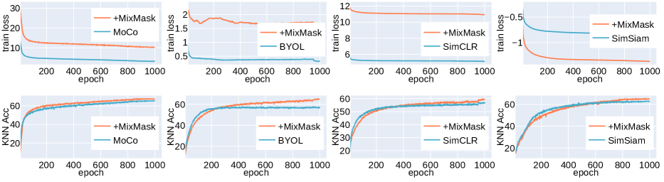
Figure 7: Training losses (top row) and k-NN evaluation accuracies (bottom row) on CIFAR-100 for experiments with 1,000 epochs for different self-supervised frameworks. MixMask (red) outperforms vanilla baseline (blue) on all frameworks by a significant margin.

Appendix D Illustrations of Different Mask Patterns

We provide additional illustrations for the different mask patterns and images generated by them. In Fig. 8 illustrations we use mask with grid size 8. All original images are sampled from ImageNet-1K.

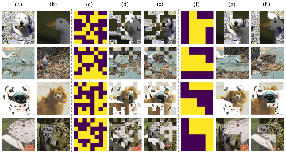
Figure 8: Illustration of different mask patterns with grid size of 8. (a) and (b) are input images. (c) is the discrete/random masking pattern, and (d) and (e) are mixed images using this mask. (f) is the blocked mask pattern, and (g) and (h) are mixed images with a blocked mask.

Appendix E Pseudocode for the Case When MixMask Used with Un-Mix

In Algorithm 1, we provide a pseudocode for the case when MixMask is used together with Un-Mix.

Algorithm 1 Pseudocode for MixMask and Un-Mix used together

⬇

1for x in train_loader:

2 x_rev = torch.flip(x[0], (0,))

3 lam_unmix = np.random.beta(1.0, 1.0)

4 # generate un-mix mixture using reverse permutation

5 if np.random.rand(1) < unmix_prob: # mixup

6 x_unmix = lam_unmix * x[0] + (1 - lam_unmix) * x_rev

7 else: # cutmix

8 x_unmix = x[0].clone()

9 bbx1, bby1, bbx2, bby2 = rand_bbox(x[0].size(), lam_unmix)

10 x_unmix[:, :, bbx1:bbx2, bby1:bby2] = x_rev[:, :, bbx1:bbx2, bby1:bby2]

11 lam_unmix = 1 - ((bbx2 - bbx1) * (bby2 - bby1) / (im_width * im_height))

12

13 index_mask = torch.randperm(len(x[0])) # generate a different random permutation

14 mask = get_mask(mask_args) # generate mask

15 x_mixmask = mask * x[0] + (1 - mask) * x[0][index_mask] # mix according a new random permutation

16 lam_mask = mask.sum() / (mask_width * mask_height) # calculate lambda for mixmask branch

17

18 output, target, output_um, output_um_flip, output_mask, output_mask_inv = model(x[0], x[1], x_unmix, x_mixmask, index_mask=index_mask)

19

20 l_o = criterion(output, target)

21 l_um = criterion(output_um, target)

22 l_um_flip = criterion(output_um_flip, target)

23 l_mask = criterion(output_mask, target)

24 l_mask_inv = criterion(output_mask_inv, target)

25

26 l = l_o + lam_unmix * l_um + (1 - lam_unmix) * l_um_flip + lam_mask * l_mask + (1 - lam_mask) * l_mask_inv # compute total loss

References

- [1] Mahmoud Assran, Mathilde Caron, Ishan Misra, Piotr Bojanowski, Florian Bordes, Pascal Vincent, Armand Joulin, Michael Rabbat, and Nicolas Ballas. Masked siamese networks for label-efficient learning. arXiv preprint arXiv:2204.07141, 2022.
- [2] Roman Bachmann, David Mizrahi, Andrei Atanov, and Amir Zamir. Multimae: Multi-modal multi-task masked autoencoders. arXiv preprint arXiv:2204.01678, 2022.
- [3] Hangbo Bao, Li Dong, and Furu Wei. Beit: Bert pre-training of image transformers. arXiv preprint arXiv:2106.08254, 2021.
- [4] Mathilde Caron, Ishan Misra, Julien Mairal, Priya Goyal, Piotr Bojanowski, and Armand Joulin. Unsupervised learning of visual features by contrasting cluster assignments. 2020.
- [5] Mathilde Caron, Hugo Touvron, Ishan Misra, Hervé Jégou, Julien Mairal, Piotr Bojanowski, and Armand Joulin. Emerging properties in self-supervised vision transformers. In Proceedings of the IEEE/CVF International Conference on Computer Vision, pages 9650–9660, 2021.
- [6] Ting Chen, Simon Kornblith, Mohammad Norouzi, and Geoffrey Hinton. A simple framework for contrastive learning of visual representations. In International conference on machine learning, pages 1597–1607. PMLR, 2020.
- [7] Ting Chen, Calvin Luo, and Lala Li. Intriguing properties of contrastive losses. Advances in Neural Information Processing Systems, 34:11834–11845, 2021.
- [8] Xinlei Chen, Haoqi Fan, Ross Girshick, and Kaiming He. Improved baselines with momentum contrastive learning. arXiv preprint arXiv:2003.04297, 2020.
- [9] Xinlei Chen and Kaiming He. Exploring simple siamese representation learning. In Proceedings of the IEEE/CVF Conference on Computer Vision and Pattern Recognition, pages 15750–15758, 2021.
- [10] Sumit Chopra, Raia Hadsell, and Yann LeCun. Learning a similarity metric discriminatively, with application to face verification. In 2005 IEEE Computer Society Conference on Computer Vision and Pattern Recognition (CVPR’05), volume 1, pages 539–546. IEEE, 2005.
- [11] Elijah Cole, Xuan Yang, Kimberly Wilber, Oisin Mac Aodha, and Serge Belongie. When does contrastive visual representation learning work? In Proceedings of the IEEE/CVF Conference on Computer Vision and Pattern Recognition, pages 14755–14764, 2022.
- [12] Jia Deng, Wei Dong, Richard Socher, Li-Jia Li, Kai Li, and Li Fei-Fei. Imagenet: A large-scale hierarchical image database. In 2009 IEEE conference on computer vision and pattern recognition, pages 248–255. Ieee, 2009.
- [13] Alexey Dosovitskiy, Lucas Beyer, Alexander Kolesnikov, Dirk Weissenborn, Xiaohua Zhai, Thomas Unterthiner, Mostafa Dehghani, Matthias Minderer, Georg Heigold, Sylvain Gelly, et al. An image is worth 16x16 words: Transformers for image recognition at scale. arXiv preprint arXiv:2010.11929, 2020.
- [14] Mark Everingham, Luc Van Gool, Christopher KI Williams, John Winn, and Andrew Zisserman. The pascal visual object classes (voc) challenge. International journal of computer vision, 88(2):303–338, 2010.
- [15] Christoph Feichtenhofer, Haoqi Fan, Yanghao Li, and Kaiming He. Masked autoencoders as spatiotemporal learners. arXiv preprint arXiv:2205.09113, 2022.
- [16] Xinyang Geng, Hao Liu, Lisa Lee, Dale Schuurams, Sergey Levine, and Pieter Abbeel. Multimodal masked autoencoders learn transferable representations. arXiv preprint arXiv:2205.14204, 2022.
- [17] Spyros Gidaris, Praveer Singh, and Nikos Komodakis. Unsupervised representation learning by predicting image rotations, 2018.
- [18] Rohit Girdhar, Alaaeldin El-Nouby, Mannat Singh, Kalyan Vasudev Alwala, Armand Joulin, and Ishan Misra. Omnimae: Single model masked pretraining on images and videos. arXiv preprint arXiv:2206.08356, 2022.
- [19] Jean-Bastien Grill, Florian Strub, Florent Altché, Corentin Tallec, Pierre Richemond, Elena Buchatskaya, Carl Doersch, Bernardo Avila Pires, Zhaohan Guo, Mohammad Gheshlaghi Azar, et al. Bootstrap your own latent-a new approach to self-supervised learning. Advances in neural information processing systems, 33:21271–21284, 2020.
- [20] Kaiming He, Xinlei Chen, Saining Xie, Yanghao Li, Piotr Dollár, and Ross Girshick. Masked autoencoders are scalable vision learners. In Proceedings of the IEEE/CVF Conference on Computer Vision and Pattern Recognition, pages 16000–16009, 2022.
- [21] Kaiming He, Haoqi Fan, Yuxin Wu, Saining Xie, and Ross Girshick. Momentum contrast for unsupervised visual representation learning. In Proceedings of the IEEE/CVF conference on computer vision and pattern recognition, pages 9729–9738, 2020.
- [22] Kaiming He, Georgia Gkioxari, Piotr Dollár, and Ross Girshick. Mask r-cnn. In Proceedings of the IEEE international conference on computer vision, pages 2961–2969, 2017.
- [23] Kaiming He, Xiangyu Zhang, Shaoqing Ren, and Jian Sun. Deep residual learning for image recognition. In Proceedings of the IEEE conference on computer vision and pattern recognition, pages 770–778, 2016.
- [24] Li Jing, Jiachen Zhu, and Yann LeCun. Masked siamese convnets. arXiv preprint arXiv:2206.07700, 2022.
- [25] Alex Krizhevsky, Geoffrey Hinton, et al. Learning multiple layers of features from tiny images. 2009.
- [26] Ya Le and Xuan Yang. Tiny imagenet visual recognition challenge. CS 231N, 7(7):3, 2015.
- [27] Tsung-Yi Lin, Michael Maire, Serge Belongie, James Hays, Pietro Perona, Deva Ramanan, Piotr Dollár, and C Lawrence Zitnick. Microsoft coco: Common objects in context. In European conference on computer vision, pages 740–755. Springer, 2014.
- [28] Zhuang Liu, Hanzi Mao, Chao-Yuan Wu, Christoph Feichtenhofer, Trevor Darrell, and Saining Xie. A convnet for the 2020s. In Proceedings of the IEEE/CVF Conference on Computer Vision and Pattern Recognition, pages 11976–11986, 2022.
- [29] Mehdi Noroozi and Paolo Favaro. Unsupervised learning of visual representations by solving jigsaw puzzles. In European conference on computer vision, pages 69–84. Springer, 2016.
- [30] Aaron van den Oord, Yazhe Li, and Oriol Vinyals. Representation learning with contrastive predictive coding. arXiv preprint arXiv:1807.03748, 2018.
- [31] Shaoqing Ren, Kaiming He, Ross Girshick, and Jian Sun. Faster r-cnn: Towards real-time object detection with region proposal networks. Advances in neural information processing systems, 28, 2015.
- [32] Pierre H Richemond, Jean-Bastien Grill, Florent Altché, Corentin Tallec, Florian Strub, Andrew Brock, Samuel Smith, Soham De, Razvan Pascanu, Bilal Piot, et al. Byol works even without batch statistics. arXiv preprint arXiv:2010.10241, 2020.
- [33] Pierre Sermanet, Corey Lynch, Yevgen Chebotar, Jasmine Hsu, Eric Jang, Stefan Schaal, and Sergey Levine. Time-contrastive networks: Self-supervised learning from video, 2018.
- [34] Zhiqiang Shen, Zechun Liu, Zhuang Liu, Marios Savvides, Trevor Darrell, and Eric Xing. Un-mix: Rethinking image mixtures for unsupervised visual representation learning. In Proceedings of the AAAI Conference on Artificial Intelligence (AAAI), 2022.
- [35] Vikas Verma, Alex Lamb, Christopher Beckham, Amir Najafi, Ioannis Mitliagkas, David Lopez-Paz, and Yoshua Bengio. Manifold mixup: Better representations by interpolating hidden states. In International Conference on Machine Learning, pages 6438–6447. PMLR, 2019.
- [36] Devesh Walawalkar, Zhiqiang Shen, Zechun Liu, and Marios Savvides. Attentive cutmix: An enhanced data augmentation approach for deep learning based image classification. arXiv preprint arXiv:2003.13048, 2020.
- [37] Sanghyun Woo, Shoubhik Debnath, Ronghang Hu, Xinlei Chen, Zhuang Liu, In So Kweon, and Saining Xie. Convnext v2: Co-designing and scaling convnets with masked autoencoders. arXiv preprint arXiv:2301.00808, 2023.
- [38] Yuxin Wu, Alexander Kirillov, Francisco Massa, Wan-Yen Lo, and Ross Girshick. Detectron2. https://github.com/facebookresearch/detectron2, 2019.
- [39] Zhenda Xie, Zheng Zhang, Yue Cao, Yutong Lin, Jianmin Bao, Zhuliang Yao, Qi Dai, and Han Hu. Simmim: A simple framework for masked image modeling. In Proceedings of the IEEE/CVF Conference on Computer Vision and Pattern Recognition, pages 9653–9663, 2022.
- [40] Sangdoo Yun, Dongyoon Han, Seong Joon Oh, Sanghyuk Chun, Junsuk Choe, and Youngjoon Yoo. Cutmix: Regularization strategy to train strong classifiers with localizable features. In Proceedings of the IEEE/CVF international conference on computer vision, pages 6023–6032, 2019.
- [41] Jure Zbontar, Li Jing, Ishan Misra, Yann LeCun, and Stéphane Deny. Barlow twins: Self-supervised learning via redundancy reduction. In International Conference on Machine Learning, pages 12310–12320. PMLR, 2021.
- [42] Hongyi Zhang, Moustapha Cisse, Yann N Dauphin, and David Lopez-Paz. mixup: Beyond empirical risk minimization. arXiv preprint arXiv:1710.09412, 2017.
- [43] Richard Zhang, Phillip Isola, and Alexei A. Efros. Colorful image colorization, 2016.