Analysis of Ring Galaxies Detected Using Deep Learning with Real and Simulated Data

Abstract

Understanding the formation and evolution of ring galaxies, galaxies with an atypical ring-like structure, will improve understanding of black holes and galaxy dynamics as a whole. Current catalogs of rings are extremely limited: manual analysis takes months to accumulate an appreciable sample of rings and existing computational methods are vastly limited in terms of accuracy and detection rate. Without a sizable sample of rings, further research into their properties is severely restricted. This project investigates the usage of a convolutional neural network (CNN) to identify rings from unclassified samples of galaxies. A CNN was trained on a sample of 100,000 simulated galaxies, transfer learned to a sample of real galaxies and applied to a previously unclassified dataset to generate a catalog of rings which was then manually verified. Data augmentation with a generative adversarial network (GAN) to simulate images of galaxies was also used. A catalog of 1151 rings was extracted with 7.4 times the precision and 15.4 times the detection rate of conventional algorithms. The properties of these galaxies were then estimated from their photometry and compared to the Galaxy Zoo 2 catalog of rings. With upcoming surveys such as the Vera Rubin Observatory Legacy Survey of Space and Time obtaining images of billions of galaxies, similar models could be crucial in classifying large populations of rings to better understand the peculiar mechanisms by which they form and evolve.

1 Introduction

Ring galaxies, galaxies with a luminous core surrounded by a disk of matter, are thought to have the potential to lead to a greater understanding of galaxy evolution as a whole. However, much still remains unknown about these galaxies. For instance, rings such as Hoag’s Object (Hoag, 1950) have not shown conclusive evidence as to how they have formed (Brosch 1985; Schweizer et al. 1987; Finkelman et al. 2011). Additionally, although we can determine that certain ring galaxies form via galaxy-galaxy collisions (Appleton 1999; Appleton & Struck-Marcell 1996), one of these galaxies, known as the Cartwheel Galaxy, hosts the most ultra-luminous X-Ray sources ever observed in a single galaxy, one of which is possibly an intermediate-mass black hole (Trinchieri, 2010). Intermediate-mass black holes are too massive to form through the collapse of a single star, and we have not yet determined their formation mechanisms (Rose et al., 2021), making studying peculiar galaxies such as the Cartwheel Galaxy crucial.

For these reasons, ring galaxies are of particular interest to study. However, only a limited number of rings have been identified. The Catalog of Southern Ring Galaxies (Buta, 1995) identified 3692 galaxies south of declination $-17^{\circ}.$ Most prominent sky surveys, including the Sloan Digital Sky Survey (SDSS; York et al. 2000) and the Panoramic Survey Telescope and Rapid Response System (Pan-STARRS; Chambers et al. 2019), only cover the sky north of around $-30^{\circ}$, making this data inconvenient for further analysis (Buta, 2017).

The Galaxy Zoo 2 project (Willett et al. 2013) alleviated this problem through the usage of data from SDSS DR7 (Abazajian et al. 2009). Morphological classifications for 304,122 galaxies were crowd-sourced from more than 50,000 contributors, and compiled into a database. 3962 of these galaxies were identified to have rings (Buta, 2017), though many were poorly resolved, and some were misclassified as a result. Less than $1\%$ of the data, in addition, had tendencies of a collisional ring galaxy (Appleton & Struck-Marcell, 1996), while most of the data involved a spiral galaxy as a primary component. Thus, it is clear that more data needs to be obtained to properly understand the formation and evolution of ring galaxies.

Over 14 months, however, were required to collect and compile the data inputted by volunteers for the 304,122 images of the Galaxy Zoo 2 project. With millions of images still left to be analyzed and upcoming digital sky surveys such as the Vera Rubin Observatory Legacy Survey of Space and Time (LSST; Ivezić et al. 2019) collecting images of billions of more galaxies, manual classification of morphologies clearly does not suffice for the dramatically increasing volume of data.

This problem inspired previous attempts to classify ring galaxies with computational analysis (e.g. Shamir 2019; Timmis & Shamir 2017). These methods, however, while simple to utilize, result in a low detection rate and a high misclassification rate. The flood fill algorithm was used, which looks for a path to the edge of the image from the center pixel, and if so, classifies a galaxy as non-ringed. As a result, objects which are not centered can result in potential problems for the model, resulting in misclassifications of potential ring candidates as non-ringed. Additionally, noise and artifacts are often misclassified as rings, as these algorithms cannot adapt to edge cases like these. Therefore, these methods do not have a large impact on existing catalogs of ring galaxies.

The analysis of large samples of galaxies with machine learning, on the contrary, can lead to a greater overall classification accuracy (Shamir, 2011), with fewer false positives, thus leading to the creation of more comprehensive catalogs of ring galaxies. Particularly, deep learning, and the continuous advancement of convolutional neural networks (CNNs; LeCun et al. 2015) has propelled efficient and accurate image classification.

Figure 1: Sky coverage of the application data. Left (a): The sky coverage before the subtraction of the sky covered by the Galaxy Zoo 2 project. Right (b): The blue represents the sky coverage of the Galaxy Zoo 2 project while the magenta represents the sky coverage of the modified catalog after removal.

Recently, CNNs have increasingly been used to classify galaxies based on their properties. For instance, Wu & Peek 2020 used a CNN to predict spectroscopic data from images of galaxies and Kim & Brunner 2016 used a CNN to distinguish between stars and galaxies. Specifically, the morphology of galaxies can also be accurately classified by these networks. One of the first applications of this was Huertas-Company et al. 2015, where a CNN was trained to classify the morphology of galaxies in the CANDELS fields with less than a $1\%$ error rate. Lanusse et al. 2017 described the creation of a CNN to identify gravitational lenses, another unique morphology, trained on a sample of 20,000 simulated galaxies. Building on this concept, Ghosh et al. 2020 trained a CNN to classify galaxies morphologically on a sample of 100,000 simulated galaxies and used a technique known as transfer learning to accurately retrain this model on a small sample of real galaxies, achieving less than a $5\%$ error rate, thus reducing the need for a larger sample size to train an accurate model.

If we want to further understand the formation and evolution of ring galaxies, it is clear that obtaining an expanded catalog of them is essential. As a CNN can achieve a low false positive rate while minimizing the misclassification of true positives, they show potential to compile large catalogs of accurately classified ring galaxies. Classifying galaxies with CNNs is additionally significantly more time efficient than manual analysis (Ghosh et al., 2020), thus showing promise for the analysis of large datasets in hours, compared to the years it would take with manual classification.

In this paper, we present a CNN with the Inception-ResNet-V2 architecture (Szegedy et al., 2016) to classify ring galaxies . This model was first trained on a sample of 100,000 simulated ringed and non-ringed galaxies and then transfer learned onto a sample of galaxies classified by Galaxy Zoo 2. Data augmentation was employed via a generative adversarial network (GAN), a deep learning architecture which uses two competing neural networks to simulate images. Then, the model was applied on a sample of $\sim 960,000$ galaxies obtained from the catalog compiled in Goddard & Shamir 2020a. The galaxies identified as rings were manually verified, and compiled into a new catalog. We then examined the specific star formation rate (SSFR), redshift, color and color-mass diagrams of these galaxies, and compared it to a sample of rings from Galaxy Zoo 2 to investigate the distinct properties of the galaxies our model detected. As spectroscopic data is not yet obtainable for many galaxies, a technique known as SED fitting (Walcher et al., 2010) was used to derive the properties of these galaxies from their photometric data.

We describe the methods used to obtain the data the model is trained, tested and applied on in $\S$ 2. In $\S$ 3, we describe the simulation of the initial training data, the selection of a model architecture, the training of the model, and the application of transfer learning. In $\S$ 4, we describe the usage of SED fitting to infer properties of the newly obtained catalog. In $\S$ 5, we present the expanded catalog of ring galaxies and their properties. Finally, in $\S$ 6 and $\S$ 7 we discuss the results and their potential applications.

2 Obtaining Data

This paper primarily discusses the usage of a CNN to detect ring galaxies in real data sets. A catalog of ring galaxies was first obtained from the Galaxy Zoo 2 project (Willett et al. 2013) to train the model. 3962 galaxies were classified as ”clean” samples of rings. As Galaxy Zoo 2 participants were shown images from the Dark Energy Camera Legacy Survey (DECaLS), images to train the model were obtained from the DESI Legacy Imaging Surveys (Dey et al., 2019) as it includes DECaLS as a primary component.

Cutouts of the training images were 256 pixels on a side. As the galaxies were arranged in descending order by angular diameter, the resolution of the images was iterated from 0.65” to 0.09” per pixel to ensure that the galaxies occupied equal areas in the frame.

The training sample of galaxies was then manually verified. Only about 3117, or 78.6%, of the initial sample of ring galaxies, was found to visually exhibit characteristics of a ring. The morphologies of contaminant galaxies were primarily elliptical galaxies and barred spiral galaxies. As described in $\S$ 3, 80% of this data was reserved for training while 20% was reserved for testing.

The model was applied to detect rings in a catalog of galaxies detected in the Pan-STARRS survey (Goddard & Shamir, 2020b). This catalog initially contained $1,685,349$ galaxies. However, the sky coverage of this catalog overlapped with that of Galaxy Zoo 2, which was used to train the model. Thus, as shown in Figure 1, the sky covered by Galaxy Zoo 2 was subtracted from that of the Pan-STARRS catalog to obtain a final catalog of $966,329$ galaxies to apply the model to. Images for these galaxies were downloaded from the DESI Legacy Imaging Surveys as previously described for the training data.

3 Creating & Training the Convolutional Neural Network

To train an accurate CNN, large data sets are typically required. However, with existing catalogs of ring galaxies being limited to only a few thousand galaxies, a different approach is required to obtain the most accurate model. A technique known as transfer learning (Zhuang et al., 2020) is used to first train the model on a sample of simulated galaxies, and the information learnt is used to retrain the model on the smaller sample of real galaxies. The steps used to train the model are shown in in Figure 2.

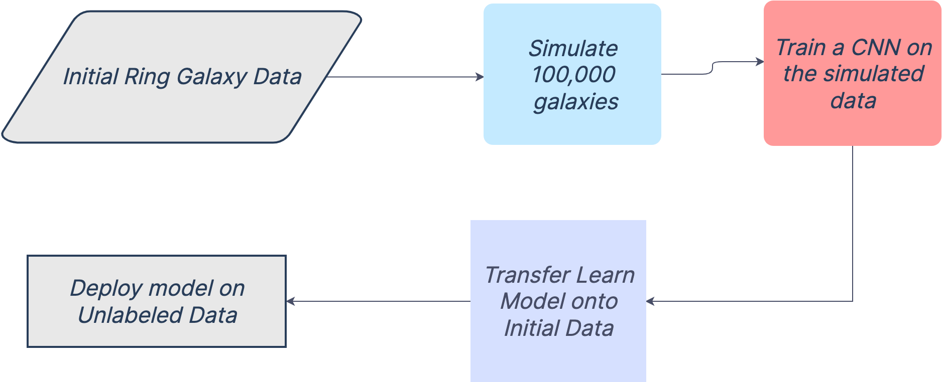
Figure 2: Workflow starting from the initial data to the final CNN. Obtaining the initial data is described in $\S$ 2. The simulation of 100,000 galaxies is described in $\S$ 3.1. The CNN trained on the simulated data is described in $\S$ 3.2. Finally, the process of transfer learning with the CNN is described in $\S$ 3.3.

Figure 3: A simulated ring galaxy and modifications to make it further resemble real data. Left (a): The simulated light profile initially created by GALFIT. Middle (b): The simulated light profile after convolution with a point spread function (PSF). Right (c): The simulated light profile after convolution with a PSF and the addition of randomized noise.

3.1 Simulating Galaxies

To simulate the initial training sample of ring galaxies, the GALFIT (Peng et al., 2002) program was used on an Ubuntu virtual machine. GALFIT is typically used to fit light profiles to astronomical objects, but in this context, as in Ghosh et al. 2020, it is used to create light profiles for randomized galaxies to be used as training data.

The training data set contained 100,000 simulated galaxies, with an even split between ringed and non-ringed galaxies. The galaxies were simulated using a Sérsic profile (Peng et al., 2010), which describes how the intensity of a galaxy varies with distance from its center. The functional form of the Sérsic profile is described by

$$\Sigma(r)=\Sigma_{e}\exp\left[-\kappa\left(\left(\frac{r}{r_{e}}\right)^{1/n}-1\right)\right].$$ (1)

$\Sigma_{e}$ represents the pixel surface brightness at the radius $r_{e}$, which represents the radius at which half of the galaxy’s flux is contained. The Sérsic index of the galaxy, $n$, controls where the light of the galaxy is concentrated, and $\kappa$ is dependent on this parameter to ensure that half of the flux stays within radius $r_{e}$ from the center.

However, a ringed structure cannot accurately be represented by one standard Sérsic function. As ring galaxies have a pronounced gap in their center, the initial Sérsic function needs to be multiplied by a hyperbolic tangent truncation function. As described in Peng et al. 2010, this is given by:

$$0.5\left(\tanh\left[\left(2-B\right)\frac{r}{r_{break}}+B\right]+1\right)$$ (2)

where

$$B=2.65-4.98\left(\frac{r_{break}}{r_{break}-r_{soft}}\right).$$ (3)

In the function, $r_{break}$ represents the radius at which $99\%$ of the galaxy’s flux is enclosed while $r_{soft}$ represents the radius at which $1\%$ of the galaxy’s flux is enclosed. However, the inner core of the galaxy still needed to be represented, thus requiring a second Sérsic profile without a truncation function applied. When simulating the sample of non-ringed galaxies, only a single Sérsic profile was needed.

Table 1: Parameters to Simulate Ringed and Non-Ringed Galaxies

Component Name	Sérsic Index		Half-Light Radius	Axis Ratio	Integrated Magnitude	Break Radius	Softening Radius
			(Pixels)		(AB)	(Pixels)	(Pixels)
Ring Galaxy
Outer Ring	1.7		2.0 - 5.0	0.7 - 1.0	15.0 - 25.0	N/A	N/A
Truncation Function	N/A		N/A	0.7 - 0.9	N/A	40.0 - 60.0	24.0 - 34.0
Inner Core	3.0		8.0 - 12.0	0.5 - 0.75	-6.2 - -3.2	N/A	N/A
Non-Ringed Galaxy
Sérsic Profile	0.0 - 8.0		55.0 - 88.0	0.1 - 1.0	17.0 - 25.0	N/A	N/A

To determine the general parameters to simulate a ring galaxy, a light profile was first fit to a galaxy from the sorted Galaxy Zoo 2 catalog. This galaxy was randomly selected, and was located at R.A.: 126.77484, Decl.: 21.64528. The sky background and center for this galaxy were determined using SourceExtractor (Bertin & Arnouts, 1996), and the other parameters were estimated based on visual inspection of the image.

The parameters of the fit light profile were then used as a baseline to create a randomized, uniform, distribution of parameters for simulating ring galaxies. Additionally, parameters for simulating non-ringed galaxies were also randomly generated with a uniform distribution. These parameters are described in Table 1. Finally, the position angle of the galaxies was iterated between $-90^{\circ}$ and $90^{\circ}$.

The GalaxySim code (Ghosh et al., 2020) was used with modifications customized to the ringed galaxies parameters to create the input files for GALFIT, run GALFIT on the input files, and modify the generated images to be more realistic.

After creating the input files, GALFIT was run to create simulated light profiles. The images were then convolved with a point spread function (PSF), representing the dispersion of light caused by atmospheric disturbances and optical limitations, to be more realistic. This PSF was obtained from the galaxy used as a prototype for the simulated rings. A randomly generated array of noise pixels was then added to the simulated image to be representative of the noise that would be present in a real image. An example of these modifications is shown in Figure 3.

Following this, a Python script was created to first scale the images, keeping $99.5\%$ of the initial pixels, and then convert them from FITS to JPG files to train the model on, as this was the file format the cutouts of the real galaxies were in.

3.2 Training the Network

A CNN is a type of artificial neural network (ANN) typically applied to analyze images. The simplest type of ANN is a multilayer perceptron (MLP), shown in Figure 4. It consists of three layers - the input layer, the hidden layers, and the output layer. These layers consist of structures called neurons which are interconnected with those of the adjacent layers. These neurons each hold a value called their activation. The activations of the input neurons determine the activation of the subsequent layer, and this occurs until an activation for the output neurons are determined.

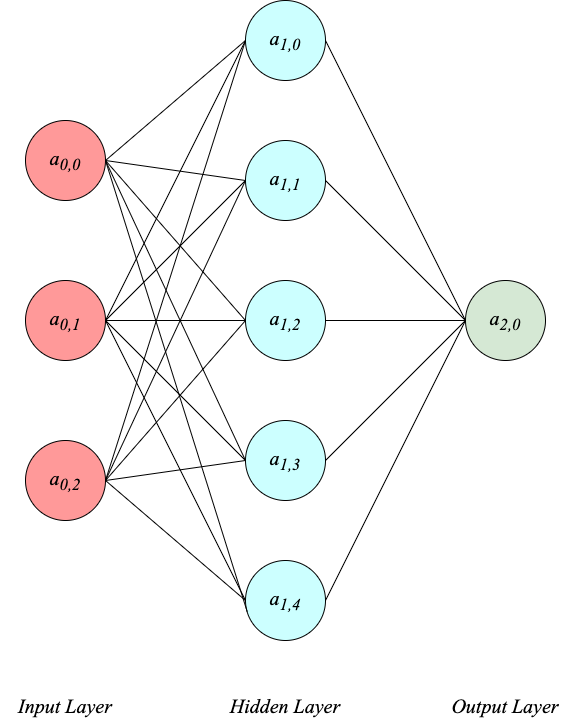
Figure 4: An illustration of a simple MLP. This contains an input layer, only one hidden layer, and an output layer.

To determine the activations of the neurons in the subsequent layer, each connection between the previous layer and the next is assigned a weight and each neuron of the next is assigned a bias. Taking first neuron in the second layer as an example, the weights of the connections are stored in a vector $w_{0}=\left(w_{0,0},w_{0,1},w_{0,2}\right)$, and the activations of the previous layer are stored in a vector $a_{0}=\left(a_{0,0},a_{0,1},a_{0,2}\right)$. The activation of this neuron is then given by

$$a_{1,0}=\sigma\left(w_{0}\cdot a_{0}+b_{1,0}\right),$$ (4)

where $b_{1,0}$ represents the bias of the neuron, and $\sigma$ represents the activation function, which is rectified linear unit (ReLU) in the CNN used to detect ring galaxies.

Table 2: Metrics for Various Models with Simulated Data

Model Name	Accuracy		Precision	Recall	$F_{1}$ Score	MCC	AUC
ResNet-50	$95.69\%$		0.912	1.0	0.9545	0.917	0.981
ResNet-101	$95.14\%$		0.912	0.997	0.953	0.906	0.975
Inception-ResNet-V2	$99.94\%$		1.0	0.998	0.999	0.998	1.0

The weights and biases are first initialized with randomized values. However, this creates a network which performs extremely poorly on an input example. Thus, these values need to be modified through a process called backpropagation. For this, a cost function is needed, which describes how poorly a given network is performing. This is typically referred to as the loss, and in our CNN, binary cross-entropy loss is used, which is given by

$$L=-\frac{1}{N}\sum_{i=1}^{N}y_{i}\cdot\log\hat{y_{i}}+(1-y_{i})\cdot\log(1-\hat{y_{i}}),$$ (5)

where N represents the number of outputs, $y_{i}$ represents the given class (1 or 0 in a binary case), and $\hat{y_{i}}$ represents the output probability. To compress the output neuron between 0 and 1, the sigmoid activation function has to be used.

To get the best possible network, L needs to be minimized. In our CNN, this is done with stochastic gradient descent (SGD; Ruder 2017), which uses several iterations in mini-batches to find a relative minimum for the loss function through modifying the weights and biases. Simple SGD is given by

$$w_{t+1}=w_{t}-\alpha\cdot dW,$$ (6)

where

$$dW=\frac{\partial L}{\partial w_{t}}.$$ (7)

In the equation, t is the time step, w is the weight of a certain connection and $\alpha$ is the learning rate, which controls how quickly the weights are changed. The same concept is also applied to modify bias. However, SGD can further be improved upon with the Adam optimizer (Kingma & Ba, 2017), which uses an adaptive learning rate, meaning that different parameters have different learning rates. This allows for faster convergence on a relative minimum of the loss function. Adam combines two other optimizers, Momentum and RMSProp. Adam is given by

$$w_{t+1}=w_{t}-\alpha\frac{m_{t}}{\sqrt{s_{t}+\epsilon}},$$ (8)

where

$$m_{t}=\beta_{1}\cdot m_{t-1}+(1-\beta_{1})\cdot dW$$ (9)

and

$$s_{t}=\beta_{2}\cdot s_{t-1}+(1-\beta_{2})\cdot dW^{2}.$$ (10)

$\beta_{1}$, $\beta_{2}$ and $\epsilon$ are constants which typically have values of 0.9, 0.999 and $10^{-8}$ respectively. The same concept can also be applied to find the correct value for bias.

Table 3: Metrics for Various Transfer Learned Models

Layers Unfrozen	Accuracy		Precision	Recall	$F_{1}$ Score	MCC	AUC
Output	$78.9\%$		0.680	0.699	0.689	0.530	0.841
Block B, C, Output	$89.2\%$		0.860	0.916	0.880	0.786	0.942
All (No Transfer Learning)	$85.0\%$		0.823	0.702	0.758	0.655	0.884

A CNN (Fukushima 1980; LeCun et al. 2015) is a type of ANN which is typically used to classify images. A CNN differs slightly from the basic MLP in that there are stages of pre-processing to the input where key features are extracted. First, a convolutional layer takes a 3D block of data as an input. For images, this is a 3D matrix of their pixel values. A kernel, a matrix smaller than the input, is initialized with certain values. These values can be learnt through several iterations with SGD. This kernel moves across the initial image, and the dot product between the kernel and the smaller patch of the initial image is stored in a new matrix referred to as a feature map. An activation function, ReLU in this case, can be applied along with the convolution to modify the feature map. A convolutional layer is then followed by a max-pooling layer, which slides a kernel across the feature map and stores the largest value of each patch into a newly created feature map. These layers are alternated until a sufficent abstraction of the initial image is acheived. The outputted feature maps are then inputted into a series of perceptron layers, similar to the MLP, and are reduced to an output containing a prediction as to what class the input image belongs to. The parameters for these layers are also learnt through SGD as seen with the ANN before.

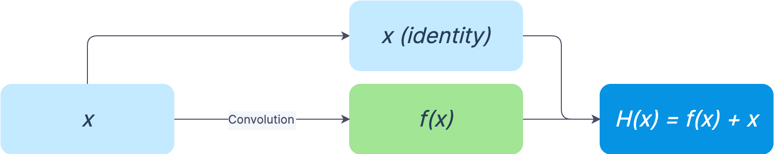
Figure 5: An illustration of the residual connections of ResNet. The identity of the initial function, $x$, is added to the feature map after convolution, $f(x)$, to produce the output.

Typically, more layers can be added to a network to increase its accuracy. For extremely deep networks, the feature maps cannot be further downsized. Then, identity mapping is required to add more layers, where convolutions are performed with a kernel which will output a feature map with the same dimensions. However, for a standard CNN, this is difficult to learn, and results in the degradation problem, where the accuracy resulting with the addition of more layers initially increases, but falls after reaching a maximum.

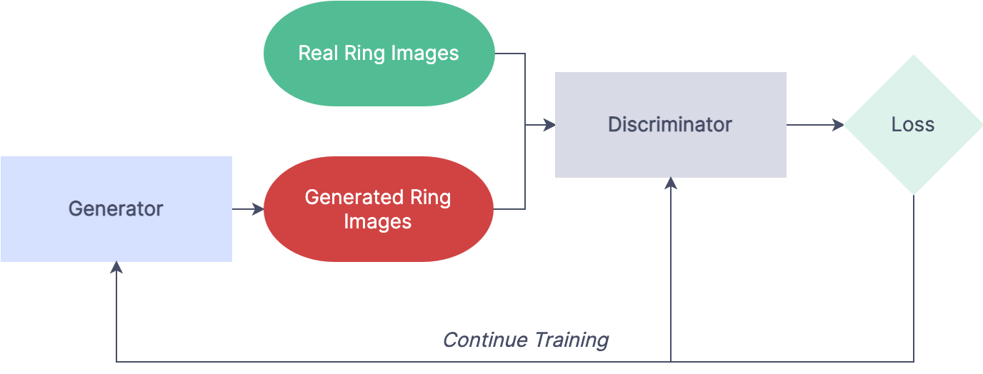
Figure 6: An illustration of the architecture of a basic GAN with a discriminator and a generator.

To combat this problem, deep residual networks (ResNets; He et al. 2015) were created. As illustrated in Figure 5, these networks take the initial feature map, and store its identity in a variable, $x$. Then, a convolution is applied to the initial feature map to produce $f(x)$. To produce the final feature map, $H(x)$, $f(x)$ is combined with $x$. These networks also help alleviate the vanishing gradient problem, where $dW$ becomes too small to make significant changes to the weights. ResNets are created by stacking many of these types of layers.

To make deeper networks, inception modules (Szegedy et al., 2014) can be used as well. These modules use a concatenation of 3x3 max pooling and 1x1, 3x3 and 5x5 convolutions within a single layer to create a feature map. Inception modules offer the advantage of allowing for the creation of a larger network and the extraction of features at various scales, thus possibly learning more features.

However, with an extremely deep network comes the risk of being too attached to the training data, known as overfitting. Thus, several methods were implemented to ensure that the risk of overfitting was very minimal on the network. The first of these methods was regularization, which adds an extra penalty term to the loss function to ensure that it does not assume extreme values. In this network, $L_{2}$ regularization (Cortes et al., 2012) was used. The modified loss function with $L_{2}$ regularization is given by

$$L_{new}=L+\frac{1}{N}\frac{\lambda}{2}\sum w_{i}^{2},$$ (11)

where the sum of the squared differences between the real and target weights is multiplied by the reciprocal of the number of outputs, $N$, and $\frac{\lambda}{2}$, where $\lambda$ is the $L_{2}$ regularization constant, which is set at $0.0001$ in the network. Additionally, data augmentation, where the initial data is transformed via several methods and expanded, was used. A scale of the images by a factor of 0.1, a shear by a factor of 1.2, a zoom by a factor of 0.25 and rotations in the range $0^{\circ}$ to $360^{\circ}$ were used.

Using the Keras API, which is built on TensorFlow, the model was created. Three models were initially tested out and evaluated. The first had the ResNet-50 (He et al., 2015) architecture, which has 50 layers and utilizes residual connections. Similarly, the second had the ResNet-101 architecture, which has 101 layers and utilizes residual connections. Finally, the third had the Inception-ResNet-V2 architecture (Szegedy et al., 2016), which has 164 layers and utilizes a combination of both inception modules and residual connections. The inception modules are organized in three blocks, A, B, and C, and each has a series of repeating layers. These networks were trained on the $100,000$ simulated images for 11 epochs with a batch size of 32 and a learning rate of $0.0001$.

To evaluate these networks, $80\%$ of this data was reserved for training, while $20\%$ was reserved for testing. Half of the data reserved for testing was used for validation, while the other half was used as a true test set, which avoids any influence the process of training might have had. The results of evaluation are described in Table 2. Using a holistic evaluation of the various metrics, Inception-ResNet-V2 was clearly the best network for the classification of the simulated ring galaxies. As a result, this network was then used for the process of transfer learning onto the real data.

3.3 Transfer Learning & GANs

To transfer the information the model learnt from the simulated data to the real data, a technique known as transfer learning (Zhuang et al., 2020) was used. To get better accuracy when limited data is available, transfer learning helps as the model is pre-trained on a different data set before training on the desired data.

Transfer learning involves freezing particular layers of the model, typically all layers excluding the output layers, and retraining the layers which remain unfrozen. The earlier layers most likely do not need retraining, as they are primarily meant to extract trivial features. A common example of transfer learning is when a model trained on the ImageNet data set is applied to a new data set. However, similar to Ghosh et al. 2020, this model is first trained on a sample of simulated galaxies resembling the real data, and then transfer learned onto the real data.

To get the best possible model, different variations of transfer learning were tested. This included retraining just the output layers, retraining inception blocks B, C, and the output layers, and retraining the entire model without using transfer learning.

The training data set contained about 9318 images, 3117 of which were ring galaxies. This data set was intentionally biased towards non-ringed galaxies to ensure that there was minimal contamination in the final sample of ringed galaxies obtained when applied on an unclassified data set. Data augmentation was used to prevent overfitting, along with early stopping, which stopped training once convergence was reached. Particularly, a generative adversarial network (GAN), the general architecture of which is shown in Figure 6, was used for data augmentation. GANs are generative models which utilize two competing neural networks: a generator is trained to generate fake data, while a discriminator is employed to distinguish generated images from real samples. As a GAN trains, the generator improves at generating fake data, and the accuracy of the discriminator starts to decrease. Due to the ability of GANs to generate realistic images, they can be used to enlarge an existing dataset.

Three different GAN architectures were tested out. This included StyleGAN-2-Ada (Karras et al., 2020), ProGAN (Karras et al., 2017) and DcGAN (Radford et al., 2015). DcGAN, the simplest out of the three, uses deep convolutional neural networks as both the discriminator and the generator. ProGAN starts from small, 4x4, images, and the model eventually ”grows” until it can generate 256x256 images. StyleGAN-2 is an extension of ProGAN, allowing more detailed features to be recreated in its generations. ADA, or adaptive discriminator augmentation, allows StyleGAN-2 to train without overfitting on small datasets. Out of the three, StyleGAN-2-Ada consistently generated the highest quality images, of which nine images out of the 20,000 generations used are shown in Figure 7.

Additionally, a differential learning rate was used. The output layers, which were completely being retrained, were assigned a learning rate of $10^{-3}$. However, the layers behind the output layers, if retrained, were assigned a learning rate of $10^{-5}$. After the model reached convergence, an extra fine-tuning step was performed. This involved unfreezing the entire model, and retraining it at the extremely low learning rate of $10^{-7}$, such that it could make minor adjustments.

The model was trained with a batch size of 32 and the early stopping had a patience of 10 epochs. The model was again trained on $80\%$ of the initial data, with $10\%$ being reserved as the validation data set and $10\%$ being reserved as the test data set. The results of the transfer learning are described in Table 3. The model where both inception block B, C and the output layers were retrained was chosen because it performed best on every metric. Then, this model was run on the unlabeled data. The galaxies classified as rings are described in $\S$ 5.

4 Inferring the properties of the galaxies with SED Fitting

Using the BAGPIPES package (Carnall et al., 2018), we are able to infer stellar population properties from photometric data. First, the photometric data from 11 bands for the identified ring galaxies is queried from the VizieR database. These bands are GALEX: FUV, NUV; PAN-STARRS: g, r, i, z, y; and WISE: W1, W2, W3 and W4. As data from only the visual part of the spectrum will likely lead to a poor approximation, UV observations from GALEX, visual observations from Pan-STARRS and infrared observations from WISE are combined. Then, along with the filter transmission curves, these observations are inputted into BAGPIPES.

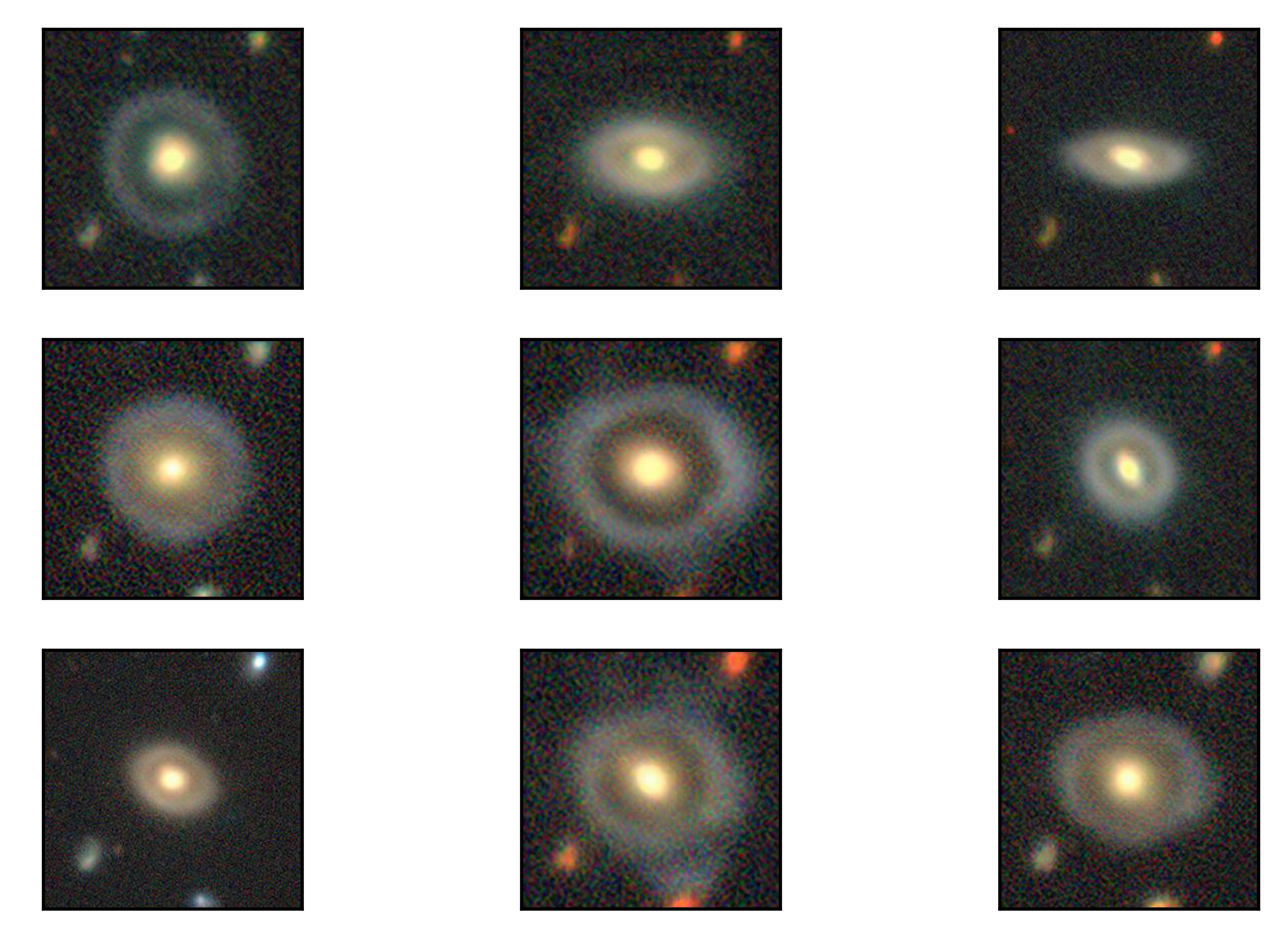
Figure 7: Nine of the GAN’s 20,000 generations. The identical background sources are discussed in $\S$ 6.

BAGPIPES is able to use the Flexible Stellar Population Synthesis package (FSPS; Conroy & Gunn 2010) to create a model with multiple stellar parameters which represents a SED. Using Bayesian inference, this model is fit to the photometric data. Bayes’ theorem, when applied in the context of SED fitting (Calistro Rivera et al. 2016; Carnall et al. 2018), states that

$$P\left(\theta|d\right)=\frac{P\left(d|\theta\right)P\left(\theta\right)}{P\left(d\right)},$$ (12)

where $\theta$ is the parameters which are used to define the model, and $d$ is the initial photometric data. $P\left(\theta|d\right)$ is also known as the posterior probability distribution, representing the information that is known with parameters $\theta$. $P\left(d|\theta\right)$ is known as the likelihood function, or $\mathcal{L}\left(d|\theta\right)$, and it represents the likelihood that the model defined by the parameters $\theta$ accurately models $d$. $P(\theta)$ represents the prior probability, or the information about the parameters already known, and $P\left(d\right)$ represents the normalization constant.

To minimize the error achieved by the model, BAGPIPES maximizes the natural log of the likelihood function (Acquaviva et al., 2011), known as the log-likelihood. This corresponds to a minimization of the $\chi^{2}$ value.

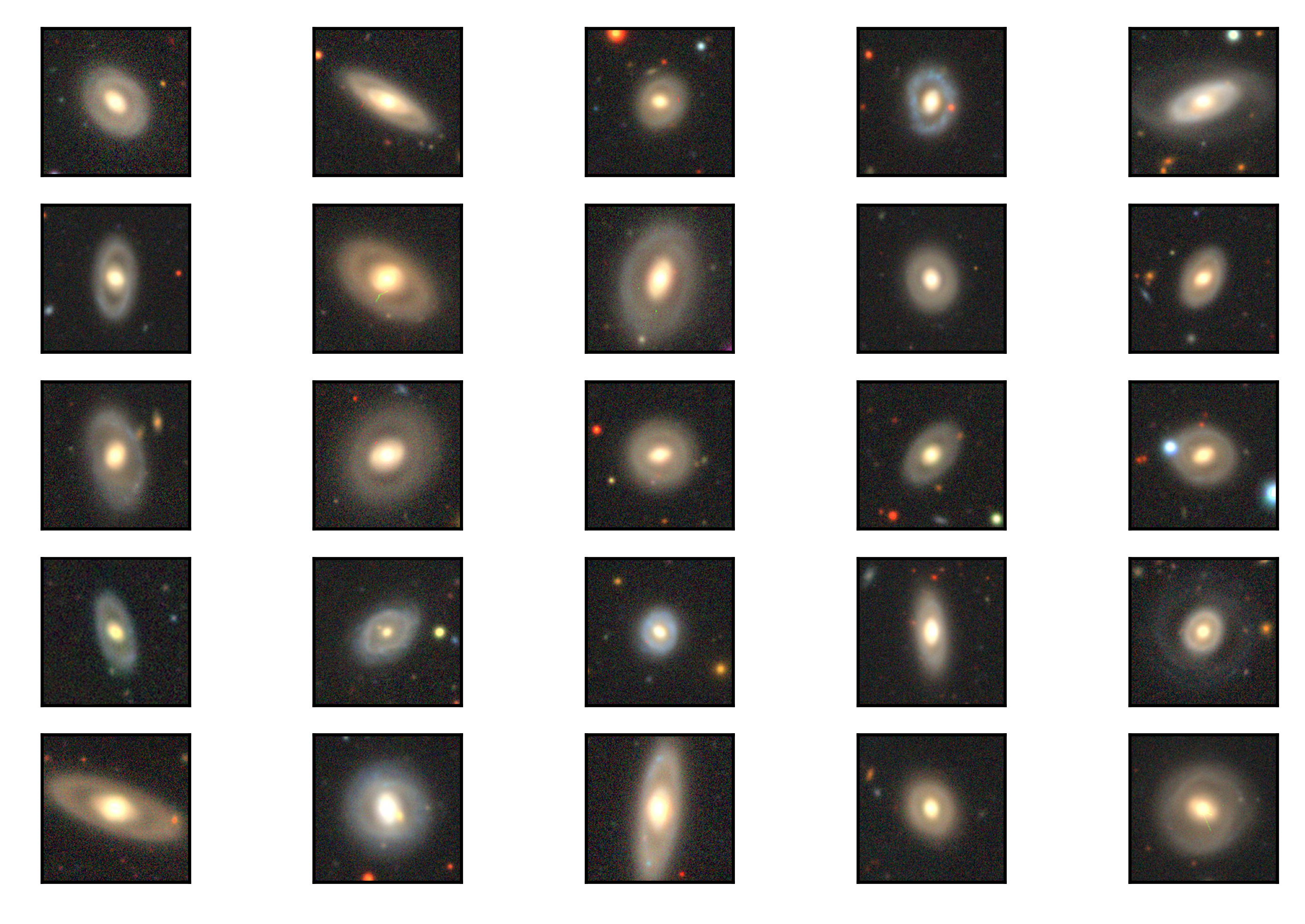
Figure 8: 25 galaxies from the catalog of 1151 rings.

Values for specific parameters, along with error, can be inferred through the posterior probability density function (PDF) of a parameter. This can be found through integrating $P\left(\theta|d\right)$ over the other parameters (Calistro Rivera et al., 2016), a process known as marginalization, given by

$$P(\theta_{1}|d)=\int P\left(\theta|d\right)d\theta_{2}d\theta_{3}\cdots d\theta_{N},$$ (13)

where $\theta_{1}$ is the parameter in question in this example. However, calculating this $N-1$ dimensional integral can get very computationally expensive, and not feasible when applied on the large scale. However, alternative methods exist to estimate this, including MultiNest (Feroz et al., 2009) and Markov Chain Monte Carlo (MCMC; Pandya et al. 2018) sampling. MultiNest is applied in this scenario to explore the parameter space and determine PDFs for each parameter, yielding the value and error for each.

Several particularly interesting parameters can then be analyzed, including the specific star formation rate (SSFR), stellar mass ($M_{*}$), and redshift. In $\S$ 5 and $\S$ 6, I will describe these results and how they can be used to infer the formation and evolution of these galaxies.

5 Results

5.1 Classification of Pan-STARRS Data

The model was applied to 966,329 previously unclassified Pan-STARRS DR1 galaxies after training. A cutoff of a $97\%$ probability to classify a galaxy as a ring was applied on the output from the final sigmoid layer of the model to ensure that the least number of non-ringed galaxies were misclassified as rings.

After the classifications of the model were manually filtered, 1151 previously unidentified ring galaxy candidates were found. These galaxies have not previously been classified as rings, making this the first time they have been recognized as rings. Figure 8 shows images of 25 galaxies from this catalog. Additionally, the application of this model to the $\sim$950,000 Pan-STARRS galaxies took only around 10 hours, markedly better than the 14 months it took Galaxy Zoo 2 volunteers to sort through the $\sim$300,000 galaxies of SDSS DR7.

The unclassified data set differed from the training, validation and confirmation data in that it was not specifically filtered to include a certain proportion of non-ringed and ringed galaxies: in a ”real” data set, less than $0.1\%$ of the galaxies are rings, while the model was trained with a 2:1 ratio of non-ringed galaxies to rings. This led to a larger proportion of non-ringed galaxies being misclassified relative to ringed galaxies: 1107 non-ringed galaxies were misclassified. However, the precision is much better than conventional computational methods regardless. Sorting through the misclassifications takes mere hours for a researcher to perform, while sorting through the entire dataset would take on the order of months.

Many of the model’s misclassifications tended to be small elliptical galaxies, like the one shown in Figure 9. The model likely identified a common feature in these galaxies which it misidentified as ringed structure, causing it to misclassify them.

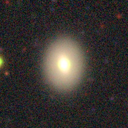
Figure 9: A galaxy misclassified as a ring.

5.2 Analysis of Properties

Through SED Fitting, the stellar mass ($M_{*}$), specific star formation rate (SSFR) and redshift of the 1151 ring galaxies were determined. Additionally, the apparent magnitudes of the galaxies were determined by

$$m=-2.5\cdot\log_{10}{\left(\frac{F}{F_{0}}\right)},$$ (14)

where $F$ is the flux density of the galaxy through a given filter and $F_{0}$ is the zero point flux density through that filter. Different colors of the galaxies, including FUV - r and g - r color, could be obtained by subtracting the apparent magnitudes of the galaxies in those filters in their respective combinations.

We compared our sample to a sample of 1054 rings from Galaxy Zoo 2. These were chosen to see how our catalog of rings differed from previous catalogs.

Using the Kolmogorov-Smirnov (KS) test, the distribution of SSFRs in our sample of ring galaxies was compared to that of the control sample of previously identified rings. The null hypothesis that both were from the same distribution was rejected with a p-value of .007, less than the p-value threshold of .05 which we had chosen.

The KS-test compares the empirical distribution function (eCDF) of both samples of galaxies. Looking at the eCDFs of the galaxies in Figure 10, it is clear that the eCDF of the Galaxy Zoo 2 rings is shifted left, indicating that the probability of finding rings from Galaxy Zoo 2 at lower SSFR values is higher than from our catalog.

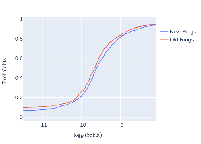
Figure 10: The eCDF of the newly identified sample of rings and the Galaxy Zoo 2 rings.

After this, the color-mass diagrams of both samples were compared against each other. On the color-mass diagram, redder galaxies (which have a lower apparent magnitude in the r-band filter) are typically older and less star forming than those which are bluer.

The FUV - r color of both our sample and the Galaxy Zoo 2 sample of rings were plotted against $\log_{10}(M_{*}/{M}_{\odot})$ on a density contour plot in Figure 11. The Galaxy Zoo 2 rings were seen to extend into higher, or redder, values, especially at lower masses. However, this effect was not seen as prominently at other wavelengths. While other colors, such as g - r and NUV - r color, were found, the most pronounced difference was seen in FUV - r color.

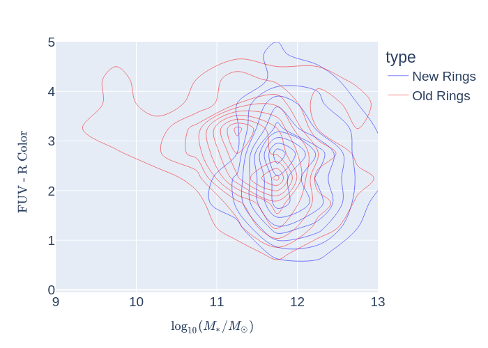
Figure 11: Color-mass diagram for FUV - r color for the newly identified sample of rings and the Galaxy Zoo 2 rings.

A frequency histogram of the masses of both samples of rings is shown in Figure 12. The newly identified sample of rings is shown to peak at a higher value of mass than the Galaxy Zoo 2 rings.

Then, a frequency histogram of the magnitudes in the r-band filter of both samples was plotted and is shown in Figure 13. The Galaxy Zoo 2 rings peak at a higher magnitude when compared with the newly identified sample.

Finally, the frequency of the redshifts of the newly identified rings were plotted as a histogram, as seen in Figure 14. The redshifts of the rings were found to range from 0.018 to 2.017, which is an extremely large range of possible values.

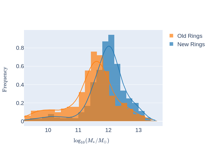
Figure 12: Frequency histogram of masses for the newly identified sample of rings and the Galaxy Zoo 2 rings.

6 Discussion

6.1 Model & Applications

When applied to the unclassified data set, the model identified 1151 ring galaxies candidates after manual verification. Compared to conventional computational models for identifying ring galaxies, this model performed considerably better.

The flood fill algorithm presented in Timmis & Shamir 2017 achieved a $6.9\%$ precision when applied to unclassified data, and 77.2 ring galaxies were detected per 1 million. On the contrary, this model achieved a $50.9\%$ precision when applied to unclassified data and detected 1191.1 ring galaxies per 1 million. This was 7.4 times the precision and 15.4 times the detection rate of previous algorithms, as shown in Table 4, dramatically improving the viability of computational methods for the detection of ring galaxies.

Ring galaxies are much harder to detect than the typical galaxy due to the wide range of morphologies they can take: some are face on and some almost lie hidden on the axis of the galaxy. Additionally, many features resemble rings, but are not actually indicative of them.

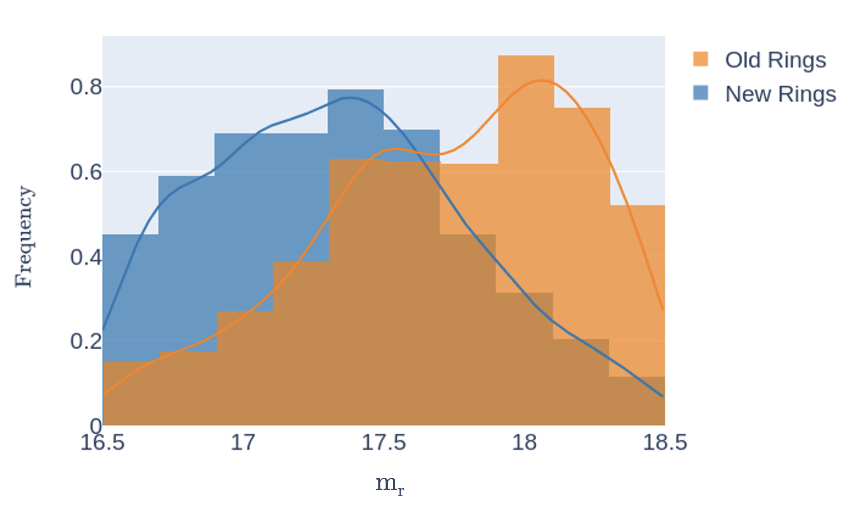
Figure 13: Frequency histogram of magnitudes in both samples of rings.

This was reflected in the misclassified sample of galaxies. Most, like that shown in Figure 9, were small elliptical galaxies. Some, however, were mergers of two galaxies and even fewer were small spiral galaxies. Although this model did not misclassify images with noise and artifacts, unlike previous models, it had trouble determining the classifications of some galaxies which exhibited certain traits of rings.

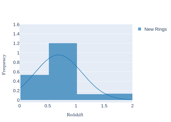
Figure 14: Frequency histogram of redshifts for newly identified rings.

One potential future step to improve the accuracy of the model could be to increase the variety of the initial simulated sample of galaxies and try to model collisional and hoag-type ring galaxies in addition to just standard rings. Multiple CNNs could also be stacked in an ”ensemble” network to ensure that the best, most supported prediction is made for every image.

Many of the GAN’s generations, as seen in Figure 7, have similar background sources, which could negativly affect the accuracy of the model. This could be alleviated in future iterations of the model by masking out the background sources of images used to train the GAN.

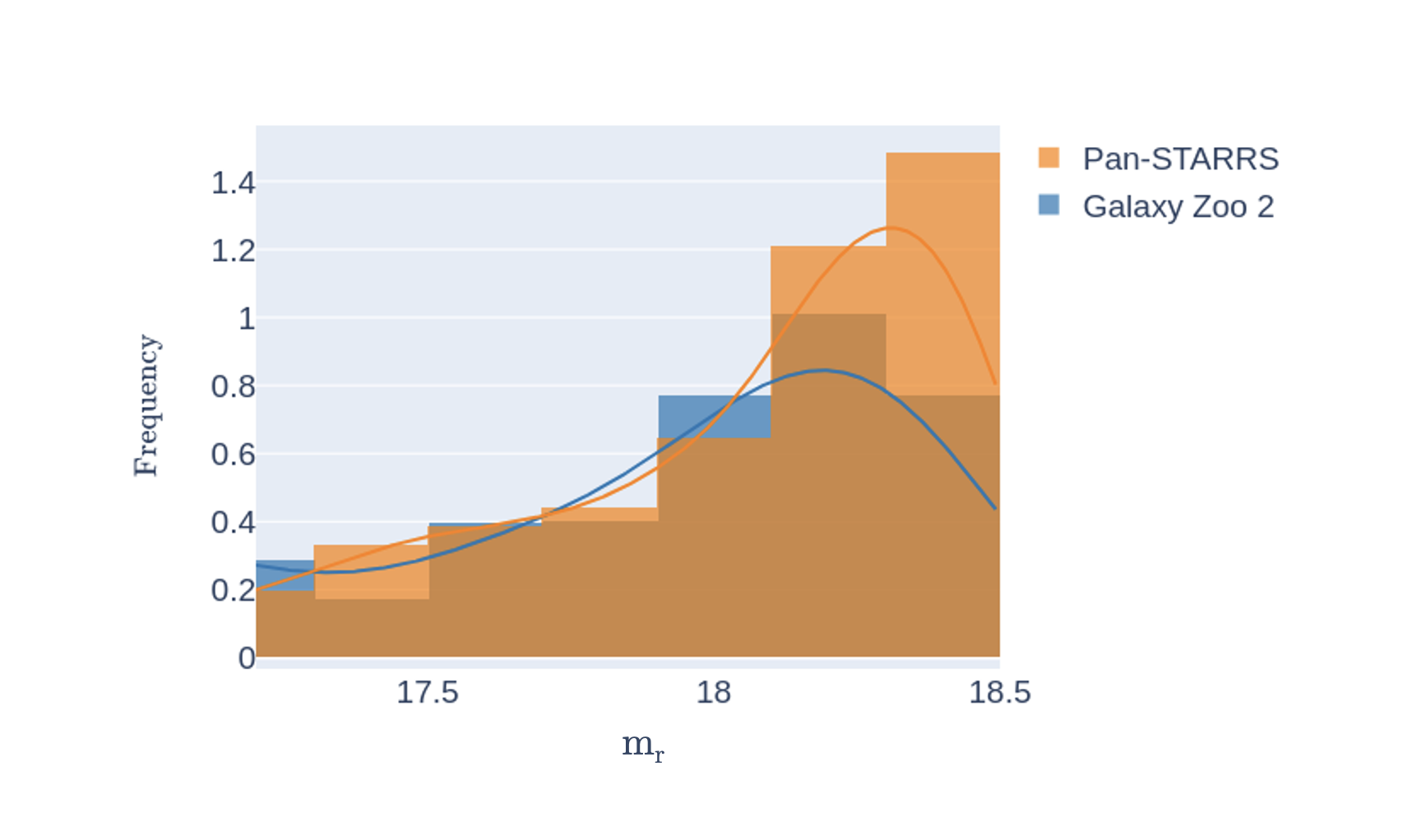
Figure 15: Frequency histogram of magnitudes for a random sample of around 1000 galaxies from the Galaxy Zoo 2 catalog and the Pan-STARRS catalog.

These results further show that a CNN can be built to detect other peculiar morphologies, for example, that of green pea galaxies. Even without large datasets, this research shows that methods such as transfer learning paired with synthetic data and GANs can allow for a competitive accuracy to be obtained.

With similar models, future sky surveys which produce billions of images, such as the LSST, can be probed for ring galaxies. After applying this model to additional data sets, any true positives identified can be used to improve the model and reduce the amount of manual sorting required. Additionally, existing sky surveys which have not yet been explored can easily be searched for thousands of more ring galaxy candidates. Without having to spend as much time to obtain an optimal sample of ring galaxies, their formation and evolution can hence be studied in more depth with larger samples.

6.2 Properties & Analysis

Table 4: Comparison of Model with Prior Literature

Algorithm	Precision	Detection Rate	Deployment Time
Our Model	$50.9\%$	1191.1 rings per 1 million galaxies	$\sim$10 hours
Prior Literature (Timmis & Shamir, 2017)	$6.9\%$	77.2 rings per 1 million galaxies	$\sim$20 days

As the Galaxy Zoo 2 catalog of ring galaxies exhibited a lower star formation rate and extended into redder values compared to the rings identified by the CNN, they could be deduced to be further in their stages of galactic evolution.

Additionally, as shown in Figure 12, the Galaxy Zoo 2 rings are less massive than the rings identified by the CNN. This could potentially indicate a bias of the model towards detecting younger, more massive galaxies compared to previous, human-compiled catalogs like Galaxy Zoo 2.

Looking at the r-band magnitudes of both samples of galaxies in Figure 13, the newly identified galaxies are seen to peak at a lower magnitude. However, as seen in Figure 15, which compares the r-band magnitudes for a random sample of rings from the Pan-STARRS and the Galaxy Zoo 2 dataset, the magnitude distributions are around the same for both catalogs. Regardless of the fact that the model was trained on the Galaxy Zoo 2 sample of rings, the human-compiled Galaxy Zoo 2 catalog identified fainter galaxies than the machine learning approach could. This could mean that in future machine-classified catalogs of galaxies, fainter galaxies that humans could have identified may potentially be misclassified. A potential reason our model performed poorly on fainter galaxies could be the fact that the initial layers of the model were only trained on the galaxies simulated via GalFit, which were much brighter than the typical galaxy with no background stars or galaxies. The classification of fainter galaxies could be improved in the future by expanding our existing data augmentation methods, employing more advanced machine learning techniques, and including even fainter galaxies in the training dataset.

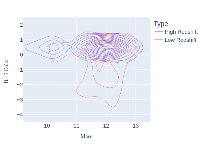
Figure 16: R - I color of low redshift rings (z $<$ 0.7) versus high redshift rings (z $>$ 0.7).

The redshift distribution of the newly identified rings was spread out from 0.018 to 2.017, while that of previous studies of rings, like Fernandez et al. 2021, was restricted to be between 0.01 $<$ z $<$ 0.1. This large range of redshifts could cause a variance of properties across our sample, which could account for the difference when analyzing properties such as SSFR and color. As shown in Figure 16, low redshift rings extend into lower R - I color values than high redshift rings. Future research could obtain more data such that it could examine and compare the properties of rings in specific redshift intervals, with a sufficient amount of samples, to ensure that variations in redshift do not affect resulting analysis.

The properties of the galaxies which were obtained in this analysis could possibly be used to conduct further investigations into these rings. The sample of 1151 newly classified rings, in addition, could be further investigated: spectroscopic data can be collected in future studies to further explore the dynamics of these galaxies. Additionally, this model could potentially be used to find rings in cosmological simulations like IllustrisTNG to better understand how they form and evolve as a whole.

7 Conclusion

In this work, we investigate the usage of a convolutional neural network to detect large catalogs of ring galaxies from sky surveys. Rings are crucial to understand more about galaxy dynamics, and current catalogs of them are extremely limited.

Our network was first trained on a sample of 100,000 synthetic galaxies - simulated using GalFit - and was then transfer learned to a sample of real galaxies consisting of 3117 rings, which was also augmented via a generative adversarial network (GAN). It was found that the Inception-ResNet V2 architecture acheived the best accuracy, and the best variation of transfer learning was when convolutional block B, C and the output layers were retrained. The source code of the model, along with a catalog of the rings discovered, is made public at https://github.com/harishk30/RingGalaxiesCNNAnalysis.

After training, this network was applied to an unclassified sample of $\sim$950,000 galaxies from Pan-STARRS, where it detected 1151 previously unclassified rings. Additionally, the network had 7.4 times the precision and 15.4 times the detection rate of conventional algorithms, showing promise for the future application of computational methods to identify ring galaxies.

After this, the properties of this sample were analyzed through SED fitting with photometric data from 11 different filters and then compared to a sample of ring galaxies from Galaxy Zoo 2. The null hypothesis that the star formation rates of both the Galaxy Zoo 2 rings and the newly identified rings were from the same distribution could be rejected with a p-value of .007. Additionally, the probability of finding the Galaxy Zoo 2 rings at lower SSFRs was higher than the newly identified sample. The Galaxy Zoo 2 rings were also found to extend to bluer colors in the FUV - r color-mass diagram.

In the future, similar models could be used to extract large catalogs of rings from future sky surveys which will collect images of billions of more galaxies. Additionally, current sky surveys which have not yet been explored could be classified by this model to compile thousands of more existing rings which have yet to be classified. The sample of 1151 rings which were identified by this model could further be explored through conducting simulations and collecting spectroscopic data, and insight about the formation and evolution of rings as a whole can be derived.

8 Acknowledgments

We would like to thank Imad Pasha and Kate Allender for their help, without which this project could not have been completed. We also thank John Franklin Crenshaw for providing his comments on our paper. The astropy, matplotlib, numpy, scipy, pandas, bagpipes and MultiNest libraries were used. JBK acknowledges support from the DIRAC Institute in the Department of Astronomy at the University of Washington. The DIRAC Institute is supported through generous gifts from the Charles and Lisa Simonyi Fund for Arts and Sciences, and the Washington Research Foundation.

References

- Abazajian et al. (2009) Abazajian, K. N., Adelman-McCarthy, J. K., Agüeros, M. A., et al. 2009, ApJS, 182, 543, doi: 10.1088/0067-0049/182/2/543
- Acquaviva et al. (2011) Acquaviva, V., Gawiser, E., & Guaita, L. 2011, Proceedings of the International Astronomical Union, 7, 42–45, doi: 10.1017/s1743921312008691
- Appleton (1999) Appleton, P. N. 1999, in Galaxy Interactions at Low and High Redshift, ed. J. E. Barnes & D. B. Sanders, Vol. 186, 97
- Appleton & Struck-Marcell (1996) Appleton, P. N., & Struck-Marcell, C. 1996, Fund. Cosmic Phys., 16, 111
- Bertin & Arnouts (1996) Bertin, E., & Arnouts, S. 1996, A&AS, 117, 393, doi: 10.1051/aas:1996164
- Brosch (1985) Brosch, N. 1985, A&A, 153, 199
- Buta (1995) Buta, R. 1995, ApJS, 96, 39, doi: 10.1086/192113
- Buta (2017) Buta, R. J. 2017, Monthly Notices of the Royal Astronomical Society, 471, 4027–4046, doi: 10.1093/mnras/stx1829
- Calistro Rivera et al. (2016) Calistro Rivera, G., Lusso, E., Hennawi, J. F., & Hogg, D. W. 2016, Astrophysical journal., 833, 98
- Carnall et al. (2018) Carnall, A. C., McLure, R. J., Dunlop, J. S., & Davé, R. 2018, Monthly Notices of the Royal Astronomical Society, 480, 4379–4401, doi: 10.1093/mnras/sty2169
- Chambers et al. (2019) Chambers, K. C., Magnier, E. A., Metcalfe, N., et al. 2019, The Pan-STARRS1 Surveys. https://arxiv.org/abs/1612.05560
- Conroy & Gunn (2010) Conroy, C., & Gunn, J. E. 2010, FSPS: Flexible Stellar Population Synthesis. http://ascl.net/1010.043
- Cortes et al. (2012) Cortes, C., Mohri, M., & Rostamizadeh, A. 2012, L2 Regularization for Learning Kernels. https://arxiv.org/abs/1205.2653
- Dey et al. (2019) Dey, A., Schlegel, D. J., Lang, D., et al. 2019, The Astronomical Journal, 157, 168, doi: 10.3847/1538-3881/ab089d
- Fernandez et al. (2021) Fernandez, J., Alonso, S., Mesa, V., Duplancic, F., & Coldwell, G. 2021, Astronomy & Astrophysics, 653, A71, doi: 10.1051/0004-6361/202141208
- Feroz et al. (2009) Feroz, F., Hobson, M. P., & Bridges, M. 2009, Monthly Notices of the Royal Astronomical Society, 398, 1601–1614, doi: 10.1111/j.1365-2966.2009.14548.x
- Finkelman et al. (2011) Finkelman, I., Moiseev, A., Brosch, N., & Katkov, I. 2011, Monthly Notices of the Royal Astronomical Society, 418, 1834–1849, doi: 10.1111/j.1365-2966.2011.19601.x
- Fukushima (1980) Fukushima, K. 1980, Biological Cybernetics, 36, 193, doi: 10.1007/bf00344251
- Ghosh et al. (2020) Ghosh, A., Urry, C. M., Wang, Z., et al. 2020, The Astrophysical Journal, 895, 112
- Goddard & Shamir (2020a) Goddard, H., & Shamir, L. 2020a, The Astrophysical Journal Supplement Series, 251, 28, doi: 10.3847/1538-4365/abc0ed
- Goddard & Shamir (2020b) —. 2020b, The Astrophysical Journal Supplement Series, 251, 28, doi: 10.3847/1538-4365/abc0ed
- He et al. (2015) He, K., Zhang, X., Ren, S., & Sun, J. 2015, Deep Residual Learning for Image Recognition. https://arxiv.org/abs/1512.03385
- Hoag (1950) Hoag, A. A. 1950, ApJ, 55, 170
- Huertas-Company et al. (2015) Huertas-Company, M., Gravet, R., Cabrera-Vives, G., et al. 2015, The Astrophysical Journal Supplement Series, 221, 8, doi: 10.1088/0067-0049/221/1/8
- Ivezić et al. (2019) Ivezić, Ž., Kahn, S. M., Tyson, J. A., et al. 2019, ApJ, 873, 111, doi: 10.3847/1538-4357/ab042c
- Karras et al. (2017) Karras, T., Aila, T., Laine, S., & Lehtinen, J. 2017, arXiv preprint arXiv:1710.10196
- Karras et al. (2020) Karras, T., Aittala, M., Hellsten, J., et al. 2020, Advances in Neural Information Processing Systems, 33, 12104
- Kim & Brunner (2016) Kim, E. J., & Brunner, R. J. 2016, Monthly Notices of the Royal Astronomical Society, 464, 4463–4475, doi: 10.1093/mnras/stw2672
- Kingma & Ba (2017) Kingma, D. P., & Ba, J. 2017, Adam: A Method for Stochastic Optimization. https://arxiv.org/abs/1412.6980
- Lanusse et al. (2017) Lanusse, F., Ma, Q., Li, N., et al. 2017, Monthly Notices of the Royal Astronomical Society, 473, 3895–3906, doi: 10.1093/mnras/stx1665
- LeCun et al. (2015) LeCun, Y., Bengio, Y., & Hinton, G. 2015, nature, 521, 436
- Pandya et al. (2018) Pandya, V., Romanowsky, A. J., Laine, S., et al. 2018, ApJ, 858, 29, doi: 10.3847/1538-4357/aab498
- Peng et al. (2002) Peng, C. Y., Ho, L. C., Impey, C. D., & Rix, H.-W. 2002, The Astronomical Journal, 124, 266–293, doi: 10.1086/340952
- Peng et al. (2010) —. 2010, The Astronomical Journal, 139, 2097–2129, doi: 10.1088/0004-6256/139/6/2097
- Radford et al. (2015) Radford, A., Metz, L., & Chintala, S. 2015, arXiv preprint arXiv:1511.06434
- Rose et al. (2021) Rose, S. C., Naoz, S., Sari, R., & Linial, I. 2021, The Formation of Intermediate Mass Black Holes in Galactic Nuclei. https://arxiv.org/abs/2201.00022
- Ruder (2017) Ruder, S. 2017, An overview of gradient descent optimization algorithms. https://arxiv.org/abs/1609.04747
- Schweizer et al. (1987) Schweizer, F., Ford, W. Kent, J., Jedrzejewski, R., & Giovanelli, R. 1987, ApJ, 320, 454, doi: 10.1086/165562
- Shamir (2011) Shamir, L. 2011, The Astrophysical Journal, 736, 141, doi: 10.1088/0004-637x/736/2/141
- Shamir (2019) —. 2019, Monthly Notices of the Royal Astronomical Society, 491, 3767–3777, doi: 10.1093/mnras/stz3297
- Szegedy et al. (2016) Szegedy, C., Ioffe, S., Vanhoucke, V., & Alemi, A. 2016, Inception-v4, Inception-ResNet and the Impact of Residual Connections on Learning. https://arxiv.org/abs/1602.07261
- Szegedy et al. (2014) Szegedy, C., Liu, W., Jia, Y., et al. 2014, Going Deeper with Convolutions. https://arxiv.org/abs/1409.4842
- Timmis & Shamir (2017) Timmis, I., & Shamir, L. 2017, A catalog of automatically detected ring galaxy candidates in PanSTARRS. https://arxiv.org/abs/1706.03873
- Trinchieri (2010) Trinchieri, F. P. A. W. G. 2010, Chandra observations of the ULX N10 in the Cartwheel galaxy. https://arxiv.org/abs/1003.4671
- Walcher et al. (2010) Walcher, J., Groves, B., Budavári, T., & Dale, D. 2010, Astrophysics and Space Science, 331, 1–51, doi: 10.1007/s10509-010-0458-z
- Willett et al. (2013) Willett, K. W., Lintott, C. J., Bamford, S. P., et al. 2013, Monthly Notices of the Royal Astronomical Society, 435, 2835–2860, doi: 10.1093/mnras/stt1458
- Wu & Peek (2020) Wu, J. F., & Peek, J. E. G. 2020, Predicting galaxy spectra from images with hybrid convolutional neural networks. https://arxiv.org/abs/2009.12318
- York et al. (2000) York, D. G., Adelman, J., Anderson, John E., J., et al. 2000, AJ, 120, 1579, doi: 10.1086/301513
- Zhuang et al. (2020) Zhuang, F., Qi, Z., Duan, K., et al. 2020, A Comprehensive Survey on Transfer Learning. https://arxiv.org/abs/1911.02685