SDSS IV MaNGA: Bar pattern speed in Milky Way Analogue galaxies

Abstract

Most secular effects produced by stellar bars strongly depend on the pattern speed. Unfortunately, it is also the most difficult observational parameter to estimate. In this work, we measured the bar pattern speed of 97 Milky-Way Analogue galaxies from the MaNGA survey using the Tremaine-Weinberg method. The sample was selected by constraining the stellar mass and morphological type. We improve our measurements by weighting three independent estimates of the disc position angle. To recover the disc rotation curve, we fit a kinematic model to the H_α velocity maps correcting for the non-circular motions produced by the bar. The complete sample has a smooth distribution of the bar pattern speed ($\Omega_{Bar}=28.14^{+12.30}_{-9.55}$ km s^-1 kpc ^-1), corotation radius ($R_{CR}=7.82^{+3.99}_{-2.96}$ kpc) and the rotation rate ($\mathcal{R}=1.35^{+0.60}_{-0.40}$). We found two sets of correlations: (i) between the bar pattern speed, the bar length and the logarithmic stellar mass (ii) between the bar pattern speed, the disc circular velocity and the bar rotation rate. If we constrain our sample by inclination within $30\degree<i<60\degree$ and relative orientation $20\degree<|PA_{disc}-PA_{bar}|<70\degree$, the correlations become stronger and the fraction of ultra-fast bars is reduced from 20% to 10% of the sample. This suggest that a significant fraction of ultra-fast bars in our sample could be associated to the geometric limitations of the TW-method. By further constraining the bar size and disc circular velocity, we obtain a sub-sample of 25 Milky-Way analogues galaxies with distributions $\Omega_{Bar}=30.48^{+10.94}_{-6.57}$ km s^-1 kpc^-1, $R_{CR}=6.77^{+2.32}_{-1.91}$ kpc and $\mathcal{R}=1.45^{+0.57}_{-0.43}$, in good agreement with the current estimations for our Galaxy.

1 Introduction

Stellar bars exist in a great variety of shapes, sizes, and galactic environments. Most of their properties are strongly tied to the stellar mass and morphology of their host galaxy. For instance, the bar fraction (the likelihood of hosting a large-scale bar) and bar length are strongly dependent on the galaxy mass (Nair & Abraham, 2010; Masters et al., 2012; Erwin, 2018). Early-type galaxies host stronger bars than their late-types counterparts. They are larger in relation to their disc (Méndez-Abreu et al., 2012; Díaz-García et al., 2016a; Erwin, 2018), prolate shaped (Díaz-García et al., 2016a; Méndez-Abreu et al., 2018) and have a flat density profile (Elmegreen & Elmegreen, 1985; Kim et al., 2015). Moreover, the size ratio between the bar and the disc remains constant over the cosmic time, suggesting an efficient coupling between both structures (Pérez et al., 2012; Kim et al., 2021).

Bars are one of the main drivers of the galaxy secular evolution (Weinberg, 1985; Kormendy & Kennicutt, 2004; Sellwood, 2014; Díaz-García et al., 2016b). Numerous analytical and numerical studies show they are efficient at transferring angular momentum from their inner resonances to those outside of corotation via dynamical friction (Lynden-Bell & Kalnajs, 1972; Tremaine & Weinberg, 1984a; Athanassoula, 2003). This angular momentum is mostly absorbed by the dark matter halo (Weinberg, 1985; Debattista & Sellwood, 2000), and in a smaller fraction by the bulge (Kataria & Das, 2019).

As a result, the bar is expected to induce substantial gaseous flows to the galaxy centres (Sormani et al., 2015). Observations of barred galaxies show a clear increase in the concentration of molecular gas (Sakamoto et al., 1999; Jogee et al., 2005) and in the star formation rate (Ellison et al., 2011; Chown et al., 2019) in the central regions. If the process in not balanced with the inflow of cosmological gas, the bar can deplete the gas supply in the disc, causing the so-called “bar quenching” (Masters et al., 2012). This scenario is supported by observations of the specific star formation rate (Cheung et al., 2013), colour (Gavazzi et al., 2015; Kruk et al., 2018), gas fraction, (Newnham et al., 2020), star formation histories (Fraser-McKelvie et al., 2020) and statistical properties of the galaxies (Géron et al., 2021).

A theoretical consequence of the large scale gas flows is the flattening of the metallicity profile (Cavichia et al., 2014; Kubryk et al., 2015b). However, this behaviour does not appear in most observations (Sánchez-Blázquez et al., 2014; Pérez-Montero et al., 2016; Sánchez-Menguiano et al., 2016), and has only been observed in low luminosity (low mass) galaxies (Zurita et al., 2021).

The bar is mostly supported by regular resonant stellar orbits located inside corotation. The most important being the x1 family (Contopoulos & Papayannopoulos, 1980). Nonetheless, chaotic orbits are also important building blocks for the bar. For example, by modelling N-body simulation snapshots, various authors have shown that regular and sticky orbits can eventually transform to chaotic orbits that support the X-shaped/boxy structure (Voglis et al., 2007; Harsoula & Kalapotharakos, 2009; Chaves-Velasquez et al., 2017). Moreover, chaotic orbits near the Lagrangian points could be responsible for the support of the spiral structure according to the Manifold theory (Voglis et al., 2006; Romero-Gómez et al., 2006; Romero-Gómez et al., 2015). The strong correlation between the strengths of the bar and spiral arms suggest both structures could be intimately coupled (Salo et al., 2010; Díaz-García et al., 2019; Garma-Oehmichen et al., 2021).

The multiple resonances produced by bars and spiral arms also have a profound effect on the disc stellar orbits. Simulations show that near corotation, stars can scatter inwards or outwards without changing their orbital ellipticity in a process called “radial migration” (Sellwood & Binney, 2002; Kubryk et al., 2015a). Since stars preserve their circular orbits, this process does not contribute to the radial heating of the disc, but should affect the metallicity distribution (Martinez-Medina et al., 2017). The rearrangement of stars can also trigger the creation of moving groups (Pérez-Villegas et al., 2017) and resonant trapping stars in the disc and the stellar halo (Quillen et al., 2014; Moreno et al., 2015).

All these secular effects depend in great extent on the bar pattern speed (hereafter $\Omega_{bar}$). Unfortunately, it is the most difficult observational parameter to estimate. Most methods developed to measure $\Omega_{bar}$ require some modelling. Some use the gas flow induced by the bar, for example, by matching observations with hydrodynamical simulations (Sanders & Tubbs, 1980; Hunter et al., 1988; England et al., 1990; Weiner et al., 2001; Pérez et al., 2004; Zánmar Sánchez et al., 2008; Rautiainen et al., 2008), or studying the residual gas velocity field after subtracting a rotation model (Font et al., 2011; Font et al., 2014, 2017). Other methods are based on the location and shape of different morphological features like dark gaps in ringed galaxies (Buta, 2017; Krishnarao et al., 2022), the offset of dust lanes (Athanassoula, 1992; Sánchez-Menguiano et al., 2015), changes in the phase of spirals (Puerari & Dottori, 1997; Aguerri et al., 1998; Sierra et al., 2015) or the position of rings (Buta, 1986; Rautiainen & Salo, 2000; Patsis et al., 2003).

The only direct method for estimating $\Omega_{bar}$ is the so-called Tremaine & Weinberg (1984b) (hereafter TW) method (see Section 3). It requires the surface brightness and line-of-sight (LOS) velocity of a tracer that suffices the continuity equation. Until recently, most measurement using the TW-method were made with long-slit spectroscopy in early-type galaxies (e.g. Kent, 1987; Merrifield & Kuijken, 1995; Gerssen et al., 1999; Debattista et al., 2002; Aguerri et al., 2003; Corsini et al., 2003; Debattista & Williams, 2004; Corsini et al., 2007).

With the advent of the integral field spectroscopy technique, the TW method has been applied to an increasing number of galaxies. Aguerri et al. (2015) measured $\Omega_{bar}$ in 15 strong barred galaxies from the survey CALIFA and found no trend with the morphological type. Guo et al. (2019) used a sample of 53 galaxies from the MaNGA survey and studied the effects of the galaxy position angle and inclination on the determination of $\Omega_{bar}$ (see also Debattista (2003)). Cuomo et al. (2019) continued the measurements from Aguerri et al. (2015) within the CALIFA survey, finding weakly barred galaxies have similar values of $\Omega_{bar}$ as the strongly barred galaxies. In Garma-Oehmichen et al. (2020) (hereafter G20), we used a sample of 15 MaNGA galaxies and 3 CALIFA galaxies to study different uncertainty sources and identify systematic errors in the method. Williams et al. (2021) applied the TW-method to 19 galaxies from the PHANGS-MUSE survey. They found ISM tracers produce erroneous signals in the TW integrals because of their clumpy distribution.

The rotation rate parameter $\mathcal{R}=R_{CR}/R_{Bar}$ (the ratio between corotation and the bar radius) gives a dynamical interpretation to the bar. The physical significance of this ratio comes from the fact that the stellar orbits that support the bar cannot extend beyond corotation (Contopoulos & Papayannopoulos, 1980; Athanassoula, 1980). Thus, the faster the bar rotates in relation to the disc, the closer $\mathcal{R}$ goes to 1. This ratio is commonly used to classify bars as slow ($\mathcal{R}$ > 1.4), fast (1 < $\mathcal{R}$ < 1.4) and the theoretically un-physical ultra-fast ($\mathcal{R}$ < 1).

Recent measurements using the TW-method find that most bars are consistent with a fast classification (with a concerning amount of ultra-fast bars) (Guo et al., 2019). This has led to a growing tension with the $\Lambda$CDM cosmological framework, where bars slow down excessively because of dynamical friction with the dark matter halo (Algorry et al., 2017; Peschken & Łokas, 2019; Roshan et al., 2021a; Roshan et al., 2021b). Nonetheless, Fragkoudi et al. (2021) showed that the bars can remain fast in more baryon dominated galaxies with higher stellar-to-dark matter ratios.

The properties of the dark matter halo are incredibly important for the bar formation and evolution. Several N-body simulations have shown that more concentrated halos are able to form stronger and larger bars (Debattista & Sellwood, 1998, 2000; Athanassoula & Misiriotis, 2002). Triaxial halos can induce the formation of bars (Valenzuela et al., 2014) but produce weaker bars compared to spherical halos (Athanassoula et al., 2013). Recent works have shown the importance of the halo spin. For example, a spinning halo can effectively suppress bar formation, by being unable to absorb angular momentum with the same efficiency (Long et al., 2014; Collier et al., 2018; Rosas-Guevara et al., 2022). Spinning halos can also change the radial extent of the disc (Grand et al., 2017), affecting the bar instability criteria (Izquierdo-Villalba et al., 2022).

Several attempts have been made in the last decade to estimate $\Omega_{bar}$ in the Milky Way (MW). Arguably, the best estimations have been derived using the made-to-measure method, which matches the density of red clump giants with N-body models of barred galaxies (Portail et al., 2017; Pérez-Villegas et al., 2017; Clarke et al., 2019; Clarke & Gerhard, 2022). Other attempts have used an adaptation of the TW method (Bovy et al., 2019), or kinematic maps of disc and bulge stars, along with the continuity equation (Sanders et al., 2019). Other methods are based on N-body simulations of MW-like galaxies (Tepper-Garcia et al., 2021; Kawata et al., 2021). All these measurements seem to converge to a pattern speed of $\Omega_{bar}\sim$ 35 - 40 km s^-1 kpc^-1. This value corresponds to a corotation radius $R_{cr}\sim 5-6$ kpc, and $\mathcal{R}\sim 1.2$, therefore classifying the MW bar in the fast category.

In this paper, we tie together the bar pattern speed of our galaxy in the context of extra-galactic measurements. We choose a sample of galaxies that reassemble the Milky Way in morphology and stellar mass. In G20 we argued some uncertainties in the TW method were still not well understood (see also Discussion in Guo et al. (2019)), and many improvements could be made. In line with this, we weight various independent measurements of the disc position angle (PA), we changed the distributions for sampling various parameters and change the rotation curve model. Throughout our procedure, we highlight possible systematic errors and decisions that could be biasing our measurements. All together, this has made our measurements more robust.

We organised the paper as follows: In Section 2 we introduce the MaNGA survey and the data processing packages used. Section 3 gives an overview of the Tremaine-Weinberg method, and discuss its limitations. In Section 4 we present our sample selection. In Section 5 we show our measurement procedures and discuss the error estimation. We present the complete sample results in section 6 and discuss future improvements Section 7. Finally in Section 8 we summarise our conclusions. All Figures and relevant measurements are available at the public repository: https://github.com/lgarma/MWA_pattern_speed

2 Data

Mapping Nearby Galaxies at Apache Point Observatory (MaNGA) (Bundy et al., 2015) is the largest galaxy survey using the Integral Field Spectroscopy (IFS) technique. It observed a sample of over $10,000$ galaxies. Its main sample comprises galaxies of all morphological types (e.g. Vázquez-Mata et al., 2022), within the redshift interval $0.1<z<0.15$ and stellar masses between $10^{9}$ and $10^{12}$ $M_{\odot}$ (for details about the sample see: Wake et al., 2017). The final sample also includes objects selected as part of $20$ ancillary programs driven by specific scientific objectives (for details refer to: Abdurro’uf et al., 2021), so a small fraction contains galaxies that may lie outside the aforementioned characteristics.

The MaNGA survey is one of the three major programs of the SDSS-IV international collaboration (Blanton et al., 2017). Its observations are carried out by the Sloan 2.5 meter telescope (Gunn et al., 2006), and uses the BOSS spectrograph, which provides a spectral resolution of $R\sim 2000$ in the wave-length range $3600$ Å - $10300$ Å (Smee et al., 2013).

Its Integral Field Units (IFUs) consist of a set of 17 hexagonal fiber-bundles of five different sizes ranging from 19 to 127 fibers (Drory et al., 2015). Each fiber has a diameter of 2 arcsec. Data taking requires that these fiber bundles be plugged into previously drilled plates, whose positions correspond to the targets to be observed per night. Finally, a 3-point dithering observing strategy is used to ensure total coverage of the required field of view (Law et al., 2016a), which for the MaNGA targets vary from $\sim$1.5 to $\sim$2.5 $R_{e}$.

In this work, we use the MaNGA reduced data (see Law et al., 2016b, for details) as well as the following data products provided by the Data Analysis Pipeline (DAP) (Westfall et al., 2019): Mean flux in r-band (as a proxy of the stellar flux), stellar velocity, the H_α velocity and their respective dispersion maps. The data was accessed via the Python package Marvin (Cherinka et al., 2019). All DAP datacubes are Voronoi-binned based on the g-band weighted signal-to-noise ratio (S/N) with a target S/N of 10 per Voronoi bin. The reconstruction method minimises the spatial covariance, making the number of independent measurements similar to the number of fibers (Liu et al., 2020).

Additionally, we use Pipe3D to recover some integrated properties, including the stellar mass, molecular gas, stellar spin parameter, stellar surface density and the velocity-sigma ratio. (Sánchez et al., 2015, 2016, 2018).

We will refer to the galaxies using their MaNGA identification number, which consist of two sets of numbers (for example 8596-12704). The first set (8596) corresponds to plate id, while the second set combines the number of fibers (127) and the fiber-bundle used (04).

3 Tremaine Weinberg method

Using a tracer that follows the continuity equation and assuming a perfectly flat disc, the Tremaine & Weinberg (1984b) method estimates $\Omega_{bar}$ as the ratio between two integrals:

$$\Omega_{bar}\sin i=\frac{\langle v\rangle}{\langle x\rangle}$$ (1)

where $i$ is the galaxy inclination, and $\langle v\rangle$ and $\langle x\rangle$ are the intensity-weighted means of the line-of-sight velocity and position of the tracer respectively (Merrifield & Kuijken, 1995). In equations this is:

$$\langle v\rangle=\frac{\int_{-\infty}^{+\infty}h(y)dy\int_{-\infty}^{+\infty}V_{LOS}(x,y)\Sigma(x,y)dx}{\int_{-\infty}^{+\infty}h(y)dy\int_{-\infty}^{+\infty}\Sigma(x,y)dx}$$ (2)

$$\langle x\rangle=\frac{\int_{-\infty}^{+\infty}h(y)dy\int_{-\infty}^{+\infty}x\Sigma(x,y)dx}{\int_{-\infty}^{+\infty}h(y)dy\int_{-\infty}^{+\infty}\Sigma(x,y)dx}$$ (3)

where $(x,y)$ is the Cartesian coordinate system of the sky plane, with $x$ aligned with the line of nodes (i.e the disc position angle). $\Sigma$ is the surface brightness and $V_{LOS}$ is the velocity in the line-of-sight, of the tracer. In this work we are using the old stellar component for weighting the TW integrals, with the r-band mean flux datacube for $\Sigma$ and the stellar velocity map for $V_{LOS}$ (Westfall et al., 2019).

$h(y)$ is an arbitrary odd weight function ($h(-y)=-h(y)$). To simulate the position of $2m+1$ slits offset by a separation $y_{0}$ we use a sum of Dirac deltas $h(y)=\sum_{n=0}^{m}\delta(y-ny_{0})-\delta(y+ny_{0})$

The separation between slits $y_{0}$ should be wide enough to prevent the use of repeated information. This separation depends on the relative orientation between the slits and the Cartesian grid:

$$y0=p/\cos(\theta)$$ (4)

where $p$ is the pixel separation and $\theta$ is lowest the angle between the grid and the disc position angle (see equation 6 in G20). We choose to set the pixel separation to $p=1$ between consecutive slits.

The symmetry in $x$ and $y$ in both $\langle v\rangle$ and $\langle x\rangle$, makes all axisymmetric features to cancel out in the integration. Thus, in practice, the integration limits can be set to cover only the non-axisymmetric structure. In some galaxies, however, the IFU coverage is not enough to reach the axisymmetric disc. It is possible a systematic error could be happening in those galaxies. We cannot estimate the value of $\Omega_{bar}$ using a larger spatial coverage, but we can reduce the length of the slits to do the opposite. To get an estimate of this systematic error, we include a slits length error in our measurements.

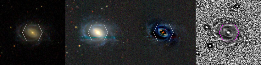
Figure 1: Image processing of the example galaxy 8596-12704. From left to right: (i) SDSS $gri$ composite colour image, (ii) DESI $grz$ composite colour image, (iii) DESI Residual image after subtracting the best Bulge/Disc 2D model of the galaxy brightness, (iv) Filter-enhanced DESI r-band image. All images include the MaNGA FoV.

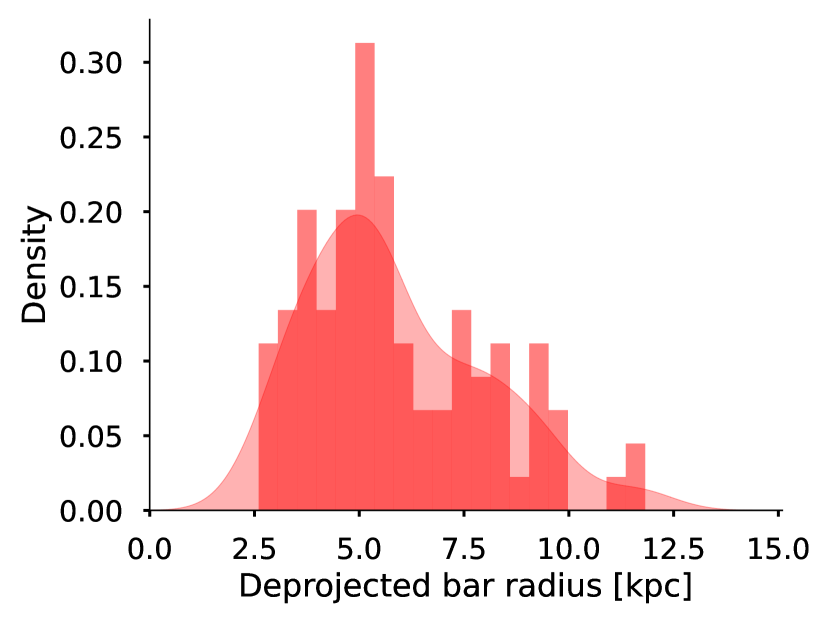
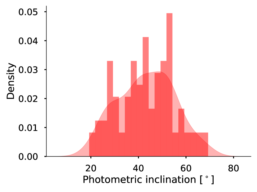
Figure 2: Statistical distribution of our sample. A kernel density estimate is used to smooth the distribution. Left panel: Logarithmic stellar mass from the NASA-Sloan Atlas catalogue. Middle panel: Deprojected bar radius, estimated from an isophotal analysis. Right panel: Disc inclination, estimated from the isophotal analysis.

The symmetry property also makes the TW method extremely sensible to the disc PA, as a wrongful estimation introduces a false signal to the integrals (Debattista, 2003). It is common that different estimates of the disc PA are not consistent within their uncertainties. This introduces another systematic error that is heavily dependent on the author’s criteria. In G20, we compared the measurements of 10 galaxies in common with Guo et al. (2019) and discussed differences in procedures to estimate $\Omega_{bar}$. The average difference in the disc PA was 3$\degree$, enough to change most measurements significantly. In G20, our measurements of $\Omega_{bar}$ differed on average 10 km s^-1 kpc^-1 when using a photometric or kinematic disc position angle. In this work, we weight the PA of three independent measurements (see section 5.1).

The TW method cannot be applied to all barred galaxies. If the bar is oriented towards the disc major or minor axis, the TW integrals will become symmetric and cancel the non-axisymmetric contributions. Thus, galaxies with mid inclinations are preferable.

4 Sample selection

By assuming that the Milky Way is not extraordinary among its peers, we can circumvent the limitation of observing our galaxy by studying galaxies with similar properties in the extra-galactic context (Boardman et al., 2020b). Throughout the literature, there have been many definitions of what makes a good Milky Way Analogue (MWA), usually based on the science goals of the study. Common limits include the stellar mass, the bulge-to-total ratio (Boardman et al., 2020a), the star formation rate (Licquia et al., 2015), galactic companions (Robotham et al., 2012; Boardman et al., 2020b) and the presence of galactic structures like the bar, spiral arms (Fraser-McKelvie et al., 2019) or an X-shaped pseudo-bulge (Georgiev et al., 2019; Kormendy & Bender, 2019).

Due to the nature of this work, we tailor our selection criteria to the stellar mass and the Hubble morphological type. The MW most prominent features include a strong peanut-shaped bar and four major spiral arms. Thus, its Hubble classification may lie somewhere between SBb and SBc (Shen & Zheng, 2020). We used the visual morphological classification reported in Vázquez-Mata et al. (2022). Figure 1 shows a mosaic containing a set of post-processed images from the SDSS and DESI Legacy Image Surveys used for morphological evaluation.

The stellar mass of the MW is estimated to be $log(M_{*}/M_{\odot})=10.75\pm 0.2$ (Licquia & Newman, 2016). We choose to extend this range to cover a complete dex in stellar mass $\log M\sim[10.3-11.3]$. Stellar masses come from a cross-match with the NASA-Sloan Atlas (NSA) catalogue (Blanton et al., 2011), using $h=0.71$ Hubble constant and a Chabrier initial mass function (Chabrier, 2003).

Using these cuts, we end up with a sample of 233 galaxies. Still, not all barred galaxies are good candidates for the TW method. The TW methods weights both the kinematic and positional data, so the inclination becomes an important selection parameter. Face-on galaxies tend to have poor kinematic data but great positional data. The opposite occurs in edge-on galaxies. To filter these galaxies, we include cuts in inclinations within the range $20\degree<i<70\degree$.

As mentioned in Section 3, the bar and the disc should not be oriented parallel nor perpendicular to each other. We included an additional cut in their relative orientation: $10\degree<|PA_{Bar}-PA_{Disc}|<80\degree$.

Finally, a good measurement with the TW method should produce a clear linear relation in between both TW-integrals. However, some galaxies do not display this trend, possibly because a lack of symmetry. We choose to remove those galaxies as well.

All together, we discarded $\sim 60\%$ of the galaxies, bringing our final sample to 97 MWA galaxies. In Figure 2 we show the stellar mass, bar radius and disc inclination distributions of the final sample. In Section 6.4 we discuss a sub-sample where we further increase the selection criteria to include the bar size and disc circular velocity to be more similar to the MW. Divided by the number of fibers, our sample contains 1, 14, 18, 12 and 52 galaxies with 19, 37, 61, 91 and 127 fibers respectively.

5 Measurements

Throughout this section, we will present our procedure using the galaxy 8596-12704 shown in Figure 1. This galaxy possesses a strong bar with an inner ring near the end of the bar. It is a grand design galaxy with two strong symmetrical arms that extend to the outer region. The MaNGA field of view only covers the bar and the inner ring.

In Figure 3 we show the corresponding isophotal profiles performed over the DESI r-band images (Dey et al., 2019). We used the ELLIPSE routine (Jedrzejewski, 1987) within the IRAF environment (Tody, 1993). To increase the signal of the outer disc, we sample the isophotes using a logarithmic step with the centre fixed.

The isophotes provide a photometric estimate of the disc PA, inclination, bar radius and bar PA. We discuss different biases in these measurements in sections 5.1 and 5.3.

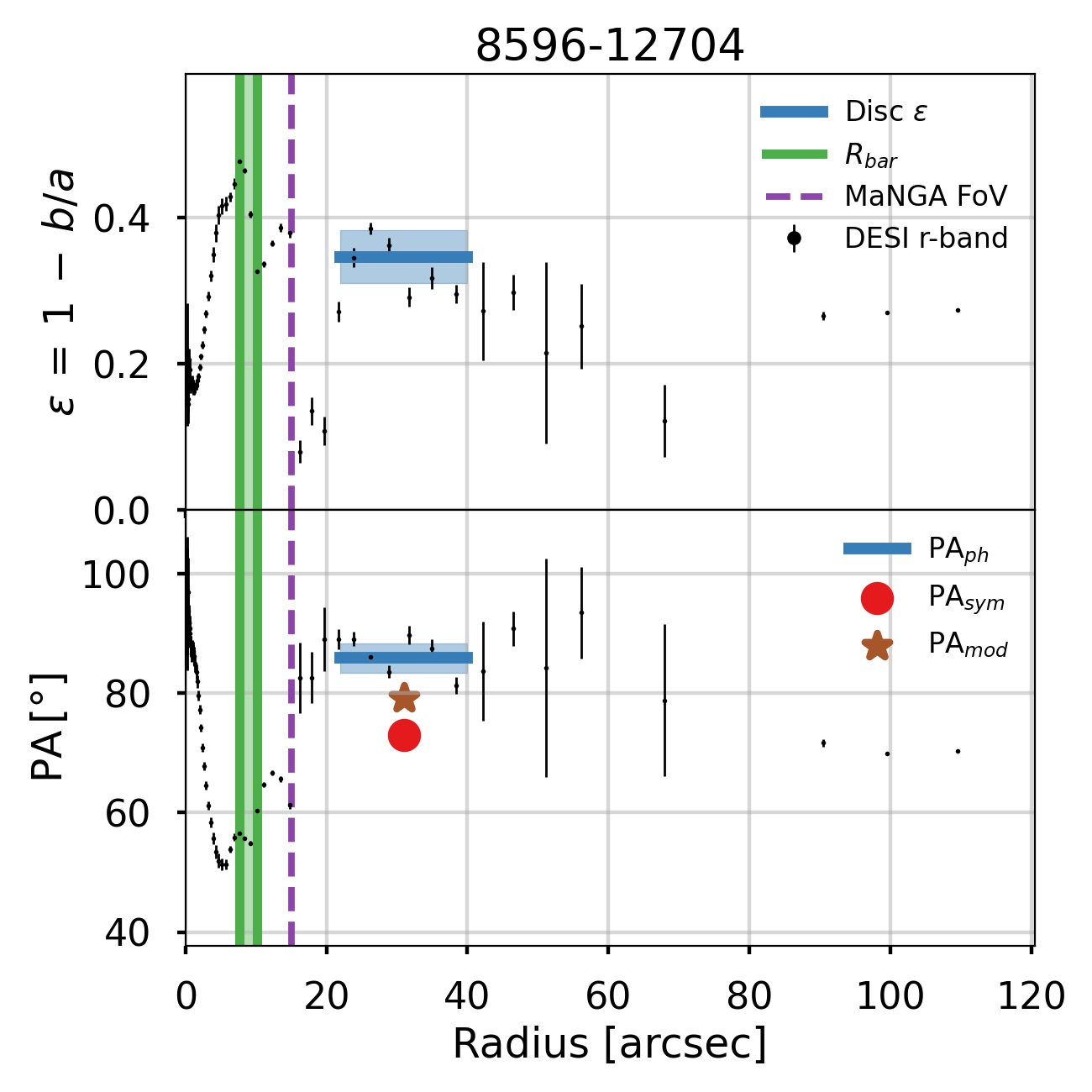
Figure 3: Ellipticity and position angle profiles of 8596-12704. The bar radius is shown with a green vertical stripe, limited by $R_{\epsilon}$ and $R_{PA}$. A sudden jump in ellipticity near the bar end occurs because of the inner ring. We estimate the disc PA using the isophotes between 22 and 40 (arcsec) shown as a blue region. For comparison, we also present the estimates after symmetrizing the stellar velocity field (PA_sym) and from the H_α kinematic model (PA_mod). In this galaxy, the three measurements of PA do not agree within uncertainties.

In Figure 4 we show the r-band surface brightness and stellar velocity maps, obtained from Marvin. We compute the TW integrals over these two maps.

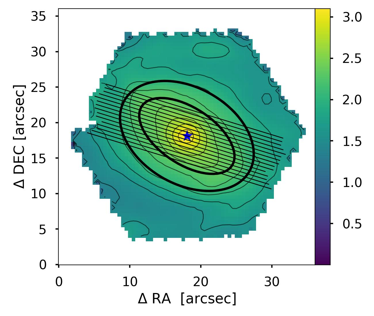
Figure 4: The r-band surface brightness and stellar velocity maps of 8596-12704. We display the surface brightness with a logarithmic scale for visualisation purposes. The bar estimates from the isophotal profiles are shown as black ellipses. We compute the TW integrals over the slits that cover the barred region.

5.1 Disc Position Angle

The disc PA is the most important parameter for making reliable measurements of $\Omega_{bar}$ with the TW method. It is well documented that few degrees of error in PA can lead to errors in $\Omega_{bar}$ of tens of percent. It has been extensively studied in simulated galaxies (Debattista, 2003; Guo et al., 2019; Zou et al., 2019) and in observations (Garma-Oehmichen et al., 2020). In G20, we measured the disc PA by using isophote profiles and by fitting a kinematic model to the H_α velocity map. After discussing the limitations in both methodologies, we concluded that the photometric estimate was more reliable as it produced more measurements that made physical sense. However, our sample was small, and our conclusion based on empirical arguments.

In this work, we use 3 independent methods for estimating the disc PA with different tracers. (i) The classical photometric approach, using the galaxy isophotes. (ii) Symmetrizing the stellar velocity map using the PAFit package (Krajnović et al., 2006). (iii) Modelling the $H_{\alpha}$ velocity maps using a modified version the package DiskFit (see Section 5.4) (Spekkens & Sellwood, 2007; Sellwood & Sánchez, 2010, Aquino-Ortíz et al. in prep.). We will refer to them as PA_ph, PA_sym and PA_mod, respectively.

Each method has biases and systematic errors that cannot be estimated from the mathematical formal errors. For example, to estimate the disc PA from isophotes, we have to assume a thin and circular disc. Strong nearby field stars, light from companion galaxies, disc warps and strong spiral arms can distort the photometric measurements. In some galaxies, the choice of the outer isophotes heavily depends on the author’s criteria. In cases of ambiguity, where the PA profile flattens in multiple sections, we use isophotes that are more similar with PA_sym and PA_mod.

The symmetrized velocity fields can be affected by local deviations from axi-symmmetry (Krajnović et al., 2011). In particular, the non-axisymmetric motions produced by the bar and other structures affect the stellar kinematics (Stark et al., 2018). In some galaxies, the IFU data only covers the central region of the galaxy, ignoring the large-scale movements of the disc.

Modelling the velocity field of the gas has the advantage of using a tracer that is not affected by the asymmetric drift present in old stellar populations. However, the $H_{\alpha}$ gas can be affected by the AGN feedback, recent galactic encounters, or episodes of strong star formation (Tsatsi et al., 2015; Stark et al., 2018). Our kinematic modelling has the additional advantage of disentangling the disc circular movements from the non-axisymmetric movements produced by the bar (Spekkens & Sellwood, 2007).

In most galaxies of our sample the three measurements are not consistent within their formal uncertainties. In Figure 5 we show the distribution of the absolute difference between the three methods for all galaxies in our sample. It is not surprising that PA_sym and PA_mod are the most similar, as both are based on the galaxy kinematics (Barrera-Ballesteros et al., 2014). Nonetheless, the average difference between both is $\sim 4.5\degree$, which is enough to produce significant differences in $\Omega_{bar}$. The large misalignment between the rotation of stars and gas is possibly provoked by environmental effects like mergers, gas accretion and interaction with nearby galaxies (Khim et al., 2020; Khim et al., 2021; Lu et al., 2021). (See also Jin et al. (2016)).

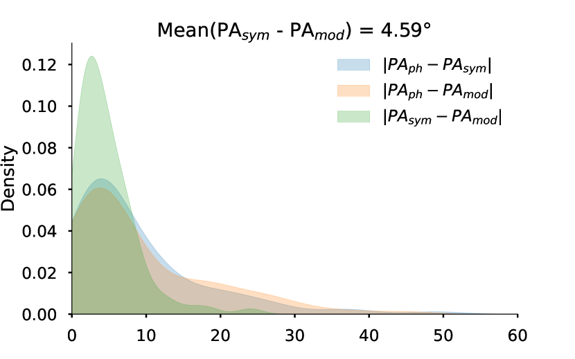
Figure 5: Distribution of the misalignment between three independent PA methods. Although the differences between PA_sym and PA_mod are smaller, they are significant enough for the TW method.

In order to weight the 3 PA measurements the following procedure was implemented: (i) We assume that the systematic errors are unknown in all our measurements and that their formal errors can be increased by using a penalisation factor. (ii) All uncertainties are increased to be at least $1\degree$. (iii) If all measures agree within their uncertainty, we proceed to use a traditional variance weighted mean. (iv) If they do not agree, we check the linearity condition between $\langle x\rangle$ versus $\langle v\rangle$ at each PA. (v) PAs that do not follow a linear trend are penalised by increasing their error by a factor of 10. (vi) The PAs that do present linearity have their errors increased to the point where they are compatible within their uncertainties. (vii) We use the variance weighted mean for our final estimation of the disc PA.

Figure 6 shows the estimates of PA for our example galaxy before and after penalising (in the top and bottom panels respectively). The differences between PA may be attributed to the strong spirals affecting the estimation of PA_ph, or to the small field of view of the IFU that only covers the barred and ringed region affecting both PA_sym and PA_mod. The strong bar of the system, can also be influencing the long scale motions of the stars and the gas.

Since these measurements are not compatible in their uncertainties, we proceed to look at the linearity of the TW diagram. Figure 8 shows the TW diagram measured at PA_sym (see Section 5.2) where the lack of a linear relation between $\langle x\rangle$ and $\langle v\rangle$ is evident. We penalise the measurement by increasing the PA_sym error by a factor 10. In comparison, both PA_mod and PA_ph satisfy the linearity requirement so we make them equal weighted. In Figure 7 we show the TW diagram measured at the mid-point between both PAs.

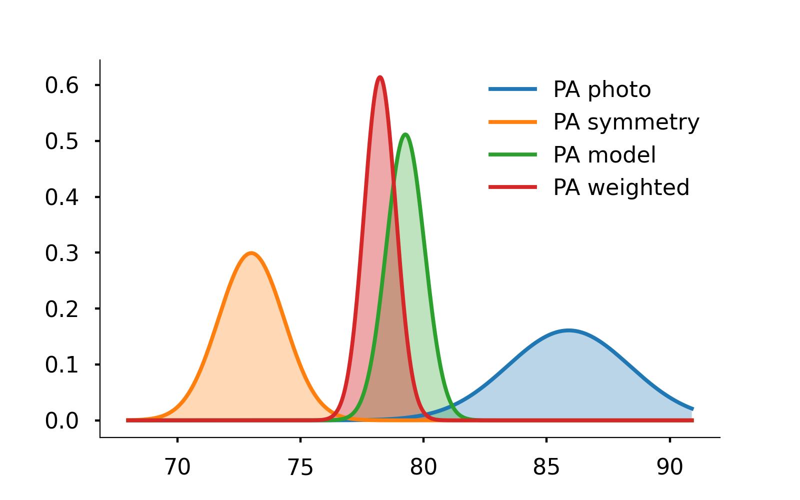
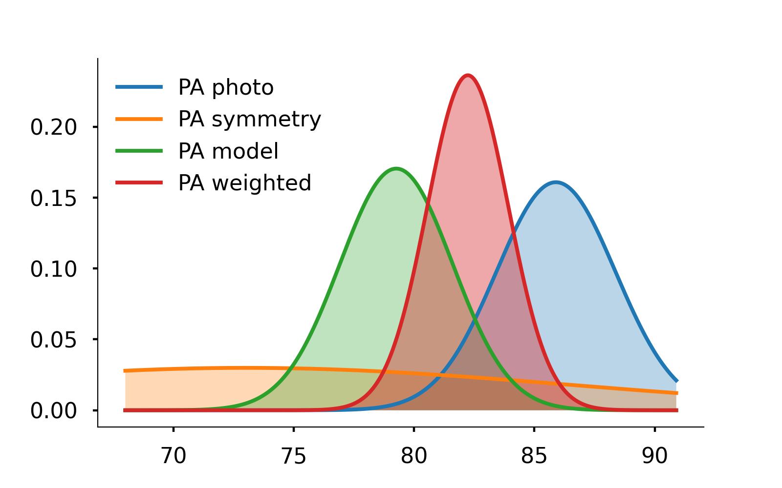
Figure 6: Weighting the 3 PA measurements. Top panel: PA measurements of 8596-12704 before penalising. The three methods do not agree within their 1-sigma uncertainties: PA_sym = $73.0\pm 1.3$, PA_mod = $79.3\pm 0.8$, PA_ph = $85.9\pm 2.48$. Bottom panel: PA measurements after penalisation. PA_sym = $73.0\pm 25.0$, PA_mod = $79.3\pm 2.5$, PA_ph = $85.9\pm 2.5$. The TW integrals at PA_sym do not follow the lineal trend (see Figure 8). Thus we choose to penalise it, and use an equal weight between PA_mod and PA_ph.

In some cases, only one estimate of the disc PA satisfies the linearity condition. In our sample, PA_sym tends to produce the better estimations of $\langle x\rangle$ and $\langle v\rangle$ (our example galaxy is an exception), followed closely by PA_mod.

5.2 Bar pattern speed

In G20, we assumed that each error source was independent and could be added in quadrature for our final estimation of $\Omega_{bar}$. This assumption was incorrect, as the behaviour of the TW integrals is non-linear, especially when considering the PA and the slit length. Instead, in this work, we choose to sample all parameters and error sources in the same Monte Carlo procedure.

We modelled the PA as a gaussian distribution with parameters from the weighted measurement of the three PA measurements described in the last section. The galaxy centre was estimated from the centre of mass of the r-band surface-brightness distribution. The mean values and co-variance matrix between $x$ and $y$ coordinates are used to model a 2-D Gaussian distribution. Considering the spatial correlations, the centre distribution looks like an ellipse oriented in the same direction as the bar.

The relative slits length (relative to the maximum slit length that fits the data) was modelled using a half-Gaussian distribution with $\mu=1$ and $\sigma=0.2$. We use this distribution to ensure most of our measurements use large slits, as the TW method suggests, but also capture some of the systematic error associated with the data coverage. In total, we draw a sample of $\times 10^{6}$ combinations of these parameters.

The number of slits varies in each galaxy as it depends on the bar coverage, orientation and the IFU size, but on average we use $\sim 15$ slits per galaxy. This results in an average of 15 $\times 10^{6}$ TW integrals, and 1 $\times 10^{6}$ measurements of $\Omega_{bar}\times\sin i$ for each galaxy.

We can separate the effects of each error source by colouring the TW integrals as a function of the random parameters. In Figure 7, we show the TW diagram of our example galaxy measured near the equal-weighted mean between PA_ph and PA_mod. Each point is a measurement made by an individual slit, with a random centre and random slit length. The slope of the plot is $\Omega_{bar}$$\times\sin i$. The three panels show the same data but are coloured using the slit number (left panel), the distance to the centre (middle panel) and the relative slit length (right panel). For the latter two panels, if the colours are randomly distributed, the measurements do not dependent on the respective error source, while stratified colours show the opposite. In this example, $\langle x\rangle$ and $\langle v\rangle$ have a strong linear relation, and low dispersion due the random parameters.

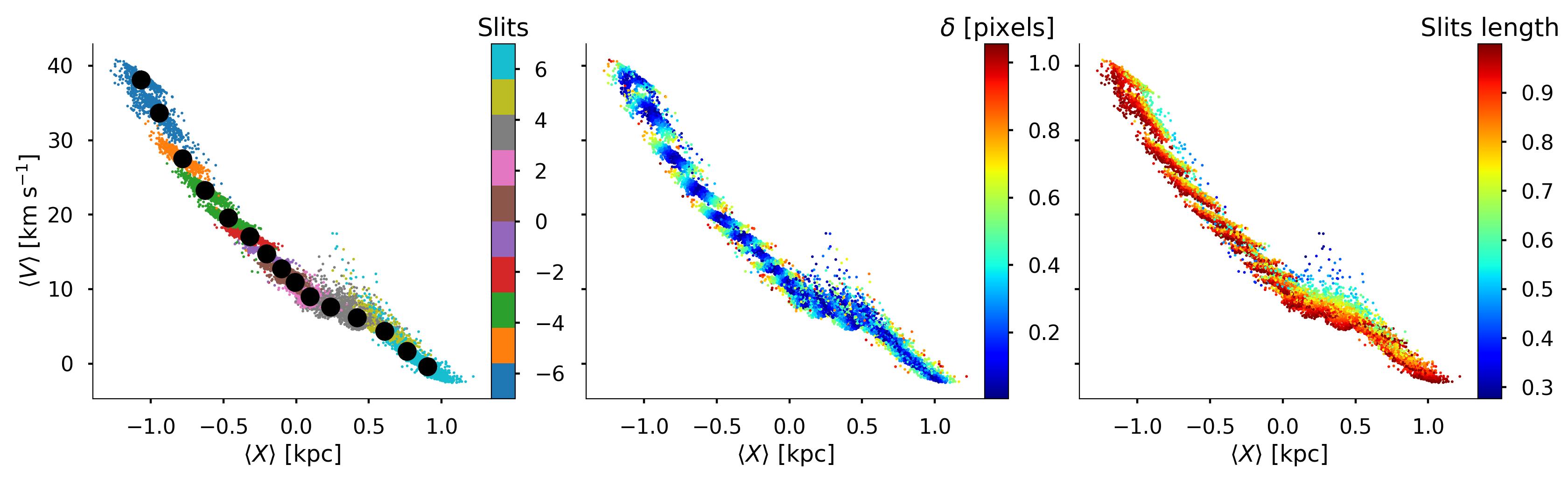
Figure 7: TW integrals $\langle x\rangle$ and $\langle v\rangle$ measured near the midpoint between PA_ph and PA_mod. Left panel: colour coded by the slit number. The black dots show the median value for each individual slit. Middle panel: coloured by the distance of the random centre to the mean centre of mass. Right panel: coloured by the relative slit length.

Figure 8 shows the same plot, but the integrals are computed near PA_sym. In this orientation, the TW integrals do not follow the linear trend, and the dispersion of each slit strongly depends on the slits length, as evidenced by the stratification in colours in the third panel. When we observe strange behaviours like this, we penalise the corresponding measurement of PA.

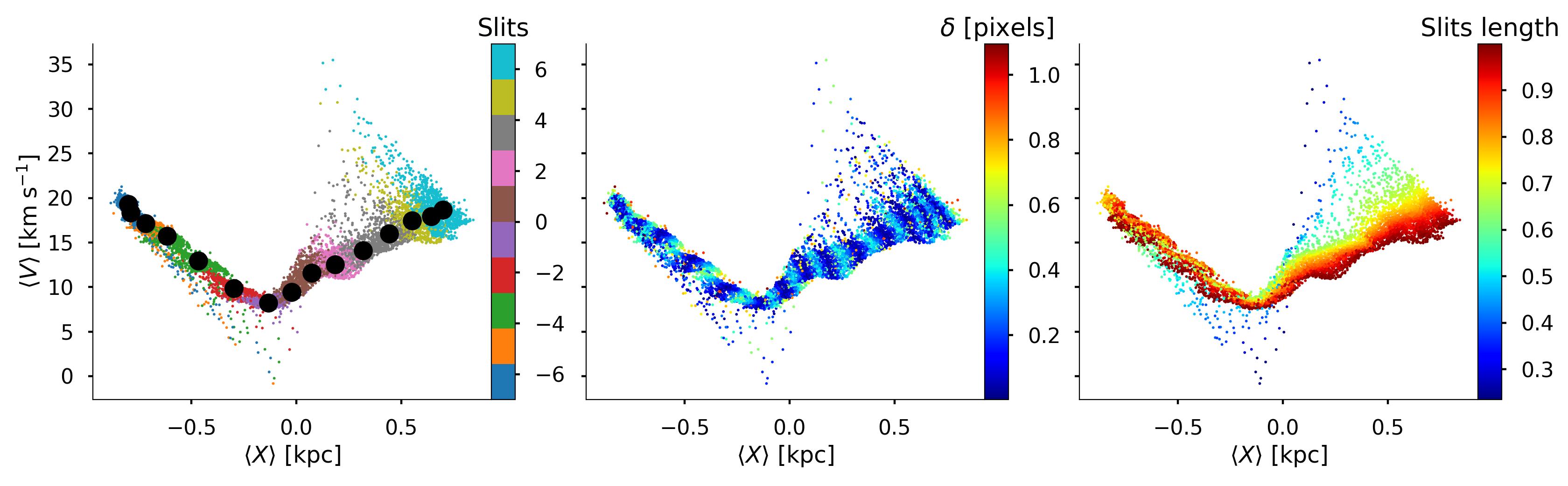
Figure 8: Same as Figure 7, but measured near PA_sym. At this orientation, the measurements highly depend on the slit length.

Figure 9 shows the relationship between $\Omega_{bar}\times\sin i$ and the disc PA for our example galaxy. Each point is the slope of a linear fit between $\langle x\rangle$ and $\langle v\rangle$ with a random centre and slit length. Again, we show three panels to disentangle the effects of each error source. The slit length becomes more important at PAs $<82\degree$ where the shorter slits produce smaller values of $\Omega_{bar}$. In this example, the most important error source is the PA (as usual), as it moves the distribution of $\Omega_{bar}$$\times\sin i$ between 10 to 25 km s^-1 kpc^-1. The third panel shows the $\chi^{2}$ of the linear fit. Notice how the linear fit is getting worse as we move to lower values of PA (closer to PA_sym).

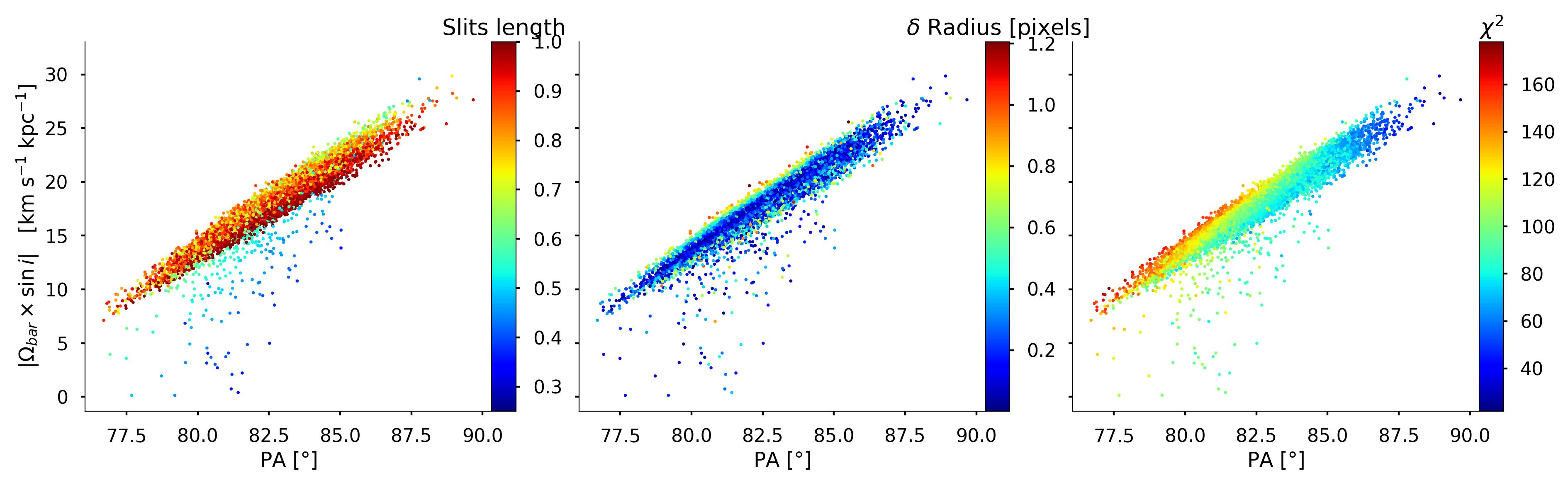
Figure 9: Bar pattern speed versus PA. Left panel: Coloured by the relative slits length. Middle panel: Coloured by distance to the centre. Third panel: Coloured by $\chi^{2}$ of the fit. Notice how the goodness of fit heavily depends on the PA.

To get the final distribution for $\Omega_{bar}$, we divide each measurement by a randomly sampled $\sin i$. The inclination is recovered from disc ellipticity using the transformation $i=\arccos(\epsilon)$. We got two measurements of $\epsilon$: (i) from the isophote analysis and (ii) from the H_α kinematic model. As with the disc PA, we expect similar biases to be affecting the disc ellipticity estimations, so we use an equally weighted ellipticity in all our galaxies. The mean and standard deviation of this estimate are used to model $\epsilon$ as a Gaussian distribution. Figure 10 shows the final distribution of $\Omega_{bar}$ for our example galaxy.

The inclination uncertainty smooths the distribution of $\Omega_{bar}$. It is important to note that a Gaussian distribution in $\epsilon$ naturally transforms into a right-skewed distribution in $\sin i$. This is relevant in galaxies with high inclination uncertainty (for example $\Delta i>6\degree$), as this results in a right-skewed distribution in $\Omega_{bar}$. We will discuss how the inclination affects the determination of $\mathcal{R}$ in Section 6.3.

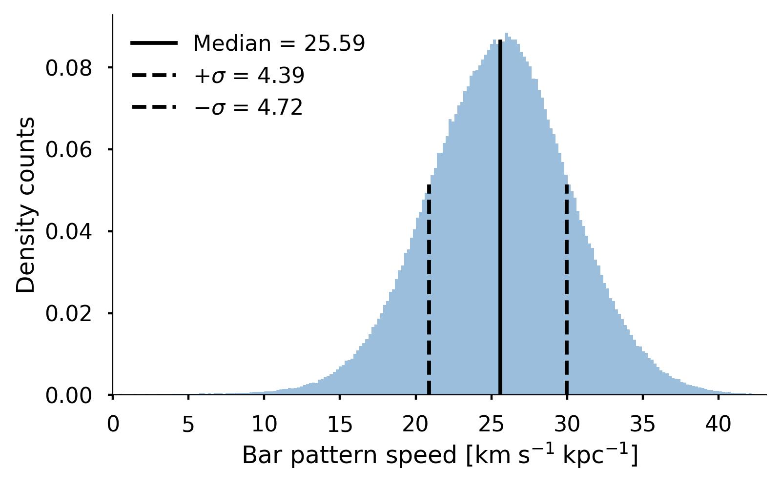
Figure 10: Bar pattern speed distribution of 8596-12704. We used a Monte Carlo procedure where we modelled the disc PA and disc ellipticity as gaussian distributions; the slits length as a half-gaussian distribution; and the galaxy centre as a 2D gaussian distribution.

5.3 Bar radius

There is no consensus on what is the best way to estimate the bar radius. Bars rarely have a well-defined boundary and are often associated with structures like bulges, spirals, rings and ansae. This makes different techniques prone to different biases.

Traditionally, the bar radius is recovered from the isophotal ellipticity and PA profiles. The barred region is characterised by an increasing ellipticity that peaks near the end of the bar and remains constant in PA. The local maximum in ellipticity (hereafter $R_{\epsilon}$) is a measurement that correlates well with visual estimates (Herrera-Endoqui et al., 2015; Díaz-García et al., 2016a). An upper limit can be defined as the radius where the PA has changed $\sim 5\degree$ from the value at $R_{\epsilon}$ (hereafter $R_{PA}$) (Aguerri et al., 2009). We can also identify the bar end with a sharp decline in the ellipticity profile. In galaxies where we observe a sharp decline in ellipticity before $R_{PA}$, we use that transition as our upper limit. Figure 3 shows both measurements with a green stripe. In Figure 4 these estimates are drawn as black ellipses.

However, the isophote technique is prone to several biases. In some galaxies, the maximum ellipticity is actually produced by open spiral arms that follow the bar. Ansae structures are relatively common in late-type galaxies, and it is not clear if they should be considered part of the bar or the disc (Martinez-Valpuesta et al., 2007). In galaxies with large bars, the choice between logarithmic or linear isophotal steps can alter the measurement of $R_{\epsilon}$ by a few arcsec. Finally, the bulge-to-total ratio (B/T) can affect the estimation in galaxies with weak exponential bars (Lee et al., 2020).

Other techniques to measure the bar radius include the ratio of the bar to inter-bar intensity, via Fourier decomposition of the light (Aguerri et al., 2000), a 2D multi-component surface brightness decomposition (fitting the light distribution of the disc + bulge + bar) (Laurikainen et al., 2005; Gadotti, 2011; Salo et al., 2015) and the maximum bar torque radius (based on the transverse-to-radial force ratio $Q_{T}$) (Sanders & Tubbs, 1980; Combes & Sanders, 1981; Díaz-García et al., 2016a; Lee et al., 2020).

In G20 we modelled the bar radius using an uniform distribution with $R_{\epsilon}$ and $R_{PA}$ as the lower and upper limits. In this work we choose to model the bar radius as a log-normal distribution, using $R_{\epsilon}$ as the mean and $R_{PA}$ as a 2-sigma upper limit. This is:

$$\mu=\log\left(R_{\epsilon}\right)$$ (5)

$$\sigma=\log\left(\sqrt{\frac{R_{PA}}{R_{\epsilon}}}\right)$$ (6)

This distribution let us explore a smaller bar radius, as suggested by Hilmi et al. (2020) and Cuomo et al. (2021). The logarithmic distribution also prevents sampling negative bar radius and, when the $\sigma/\mu$ ratio is small, the distribution resembles a Gaussian distribution.

We deproject the bar using the analytical procedure described in Gadotti et al. (2007). The method works well in galaxies with moderate inclination angles ($<60\degree$) (Zou et al., 2014), which is the case for most galaxies in our sample . The method requires the relative orientation of the bar with the disc, as well as the disc inclination angle.

5.4 Corotation radius and the H_α rotation curve model

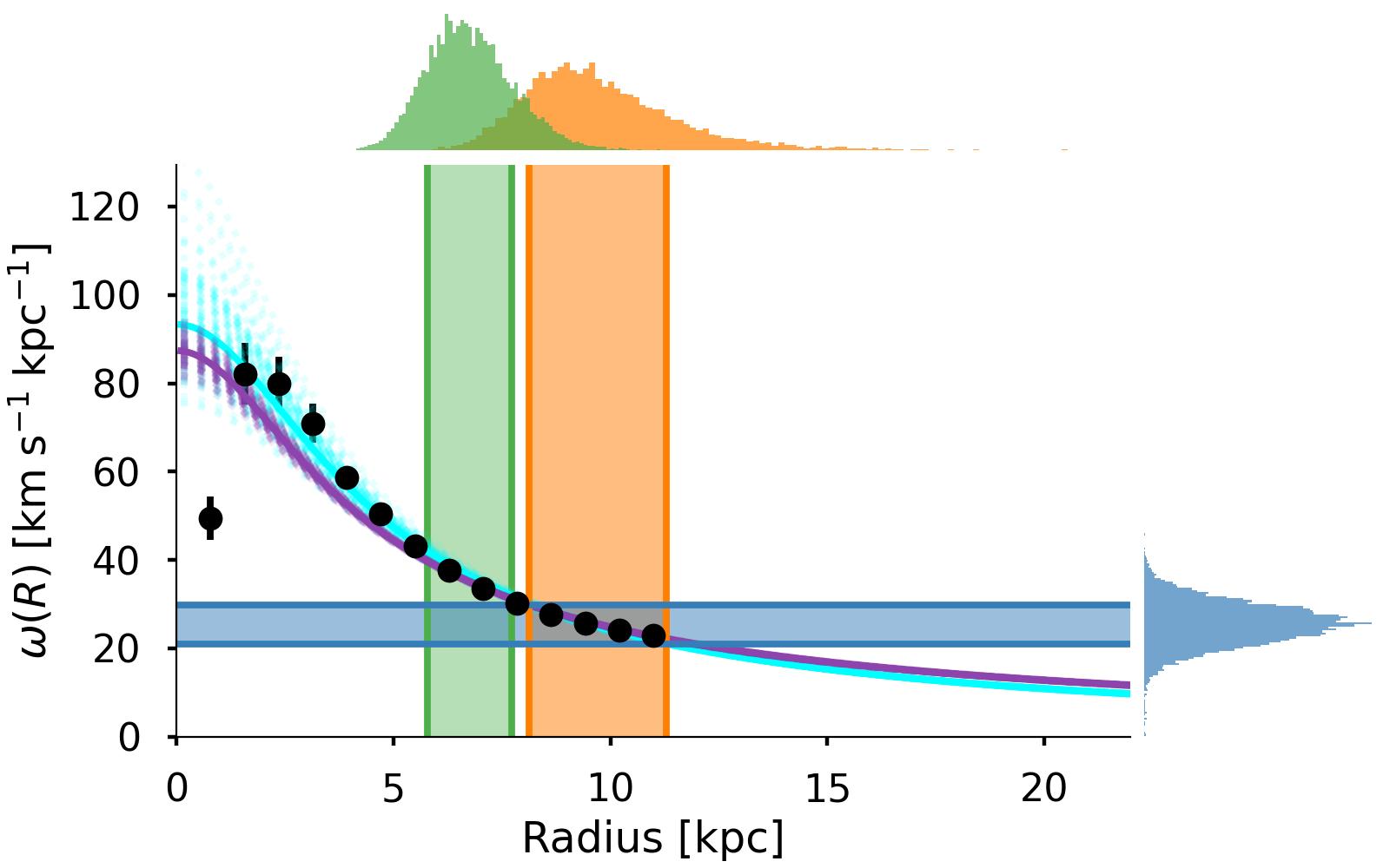
Figure 11: Rotation model of 8596-12704. Top panel: Rotation curve. The black dots show the mean circular velocity of the Diskfit model. The blue and red dots show the fitted radial and tangential non-circular motions. The cyan and purple curve are the best fit of equation 7 using $gamma$ as a free parameter or fixing it to $gamma=1$ respectively. Bottom panel: Angular velocity curve. The bar pattern speed distribution is shown in blue. The bar radius distribution is shown in green. The resulting corotation distribution is shown in orange. The projections are limited by the 1-sigma errors.

To get a reasonable measurement of corotation, we require a good estimate of the rotation curve. Several works assume a quick flattening, and estimate $R_{cr}$ as the ratio $V_{c}^{flat}/\Omega_{bar}$ where $V_{c}^{flat}$ is the flat circular velocity of the disc (Aguerri et al., 2015; Cuomo et al., 2019; Guo et al., 2019). Recovering the details in the shape of the rotation curve requires careful modelling. Massive (brighter) galaxies typically display slowly declining rotation curves, while galaxies with low masses have monotonically rising rotation curves (Persic et al., 1996; Kalinova et al., 2017). Moreover, bumps and wiggles are common features of rotation curves, that result from the perturbed kinematics of the galactic disc components. The amplitude of these wiggles varies depending on the galaxy and perturber (bar, spiral arms, satellites), and takes a proper model to be correctly represented. In G20, we got a relative difference of 21% in the $R_{cr}$ estimation between modelling the rotation curve and assuming a flat disc.

Recovering the rotation curve from 2D velocity maps is straightforward when the tracers have small departures from circular orbits (Begeman, 1987). However, stellar bars and other non-axisymmetric features can drive large non-circular motions that complicate the determination of the rotation curve (Valenzuela et al., 2007).

In this work, we use the code Diskfit that describes the velocity field with the so-called bi-symmetric model (Spekkens & Sellwood, 2007; Sellwood & Sánchez, 2010). This kinematic model assumes that most perturbations can be described by an $m=2$ order harmonic decomposition. The code yields the mean circular velocities and amplitudes of non-circular streaming velocities in the radial and tangential directions.

The code Diskfit uses a Levenberg Marquardt (LM) algorithm as a minimisation technique. However, the parameter space may have several local minimum values, where the LM routine can easily get trapped. To overcome this issue, we used a modified version that implements a Markov Chain Monte Carlo method (Aquino-Ortíz et al., in prep). The input parameters are optimised using the Metropolis-Hastings algorithm (e.g. Puglielli et al., 2010). This version has been used in recent kinematic studies (e.g. Aquino-Ortíz et al., 2018, 2020).

In most galaxies of our sample, the kinematic model is not enough to estimate $R_{cr}$. Because of the data coverage, the rotation curve only covers the central region of the galaxy, and additional modelling is required to extrapolate the outer parts. We use a 3 parameter model (Bertola et al., 1991):

$$V(r)=\frac{V_{c}r}{(r^{2}+k^{2})^{\gamma/2}}$$ (7)

where $V_{c}$ controls the amplitude, $k$ the sharpness and $\gamma$ the slope at large radius. When $\gamma>1$ the model corresponds to a declining curve and $\gamma<1$ to a rising curve. It is important to note that there is a large degeneracy between $V_{c}$ and $\gamma$, and in some galaxies, a better fit can be achieved by fixing $\gamma=1$ (a 2 parameter flat rotation model).

Some galaxies require no extrapolation, as $R_{cr}$ can be determined within the kinematic model. In those cases, we used a spline fit that recovers small details like wiggles that cannot be modelled with the parametric functions.

For each measurement of $\Omega_{bar}$ we generate a random rotation curve with the parameters of the best fit. The top panel of Figure 11 shows the rotation curve of the example galaxy. The black dots correspond to the mean circular velocity from the Diskfit model. Blue and red dots at the bottom are the m=2 radial and tangential motions, respectively. The model stops at $\sim$ 11 kpc due to the data coverage. The cyan and purple curves show random iterations of equation 7 where the difference is using $\gamma$ as a free parameter or fixing it to 1. Here, the 3 parameter model fits a declining rotation curve, while the flat model remains at $V_{c}=250$ km s^-1. At large radii, the difference between the two curves becomes more important.

The bottom panel of Figure 11 shows the angular velocity curve. The blue marginalised distribution in the right is the bar pattern speed we obtained in Figure 10. The green distribution is the bar radius we modelled in Section 5.3. The corotation radius distribution is shown in orange, and was obtained form the intersections of $\Omega_{bar}$ with the 3 parameter random angular velocity curves.

5.5 Rotation rate $\mathcal{R}$

To estimate $\mathcal{R}$ we divide each element of $R_{cr}$ with a random bar radius modelled with a log-normal distribution. The shape of $\mathcal{R}$ distribution is usually skewed to the right. It is common that galaxies with large uncertainties (in PA, inclination or bar radius) will show a large tail in $\mathcal{R}$ in the slow bar regime.

In Figure 12 we show the resulting probability distribution of the example galaxy.We estimate the probability of bar being slow, fast or ultra-fast by using the area of the probability distribution. In this particular case, the median of the distribution ($\mathcal{R}$$=1.43$) and the most probable classification (Slow = 0.52) both coincide with a slow rotating bar.

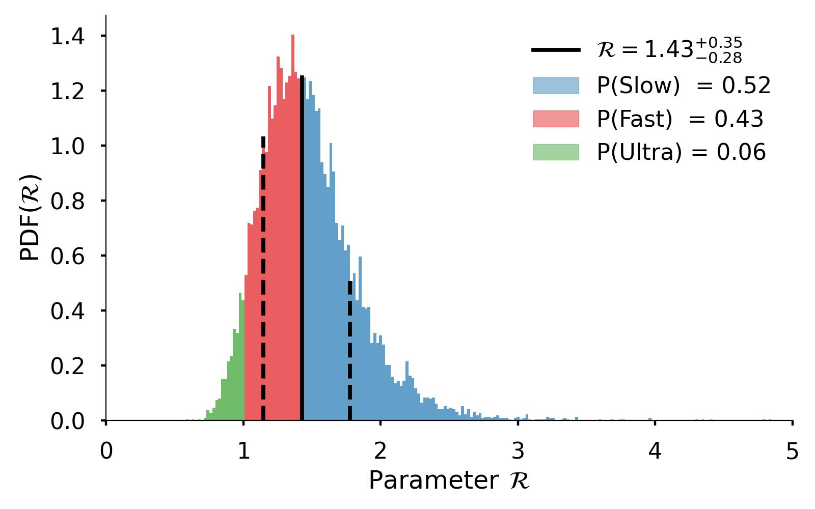
Figure 12: Rotation rate $\mathcal{R}$ of 8596-12704. The distribution is coloured using the kinematic classifications of the bar. The area under the curve of each classification is shown in the top right.

6 Results

In this section we present the statistical results of our complete sample. We include measurements of global properties from the Pipe3D package (Sánchez et al., 2018) including stellar mass, molecular gas mass, stellar spin parameter and stellar surface density.

6.1 Statistics of the full sample

Figure 13 shows the distribution of $\Omega_{bar}$, $R_{cr}$ and $\mathcal{R}$ after adding the results of the complete sample. The median relative error is 20%, 22% and 26%, respectively. This is slightly smaller than other TW based measurements. For reference, Table 1 shows the median relative errors from Aguerri et al. (2015), Guo et al. (2019) and Garma-Oehmichen et al. (2020). Nonetheless, our treatment is not free of biases, and we comment on further improvements for future measurements in Section 7.1.

Work	$\Omega_{bar}$	$R_{cr}$	$\mathcal{R}$
(1)	(2)	(3)	(4)
Aguerri et al. 2015	35%	43%	39%
Guo et al. 2019	24%	28%	37%
Garma et al. 2020	18%	30%	30%
This work	20%	22%	26%

Table 1: Median relative errors in TW based measurements. For all works we used the light-weighted results at the photometric PA orientation. Col. (1) Work. Col. (2) Relative error in the bar pattern speed. Col. (3) Relative error in corotation radius. Col. (4) Relative error in rotation rate.

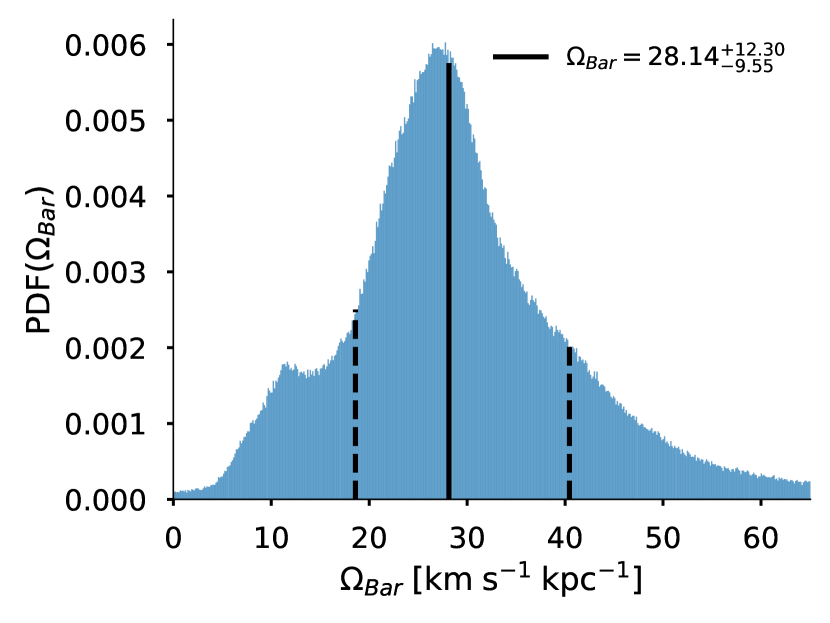
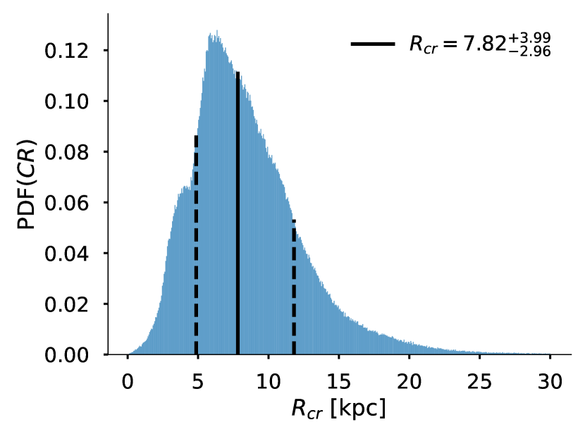
Figure 13: Distributions of the bar properties for the complete sample of galaxies. Top panel: Bar pattern speed. Middle panel: Corotation radius. Bottom panel: Rotation rate $\mathcal{R}$.

Most of our sample is near the border between fast and slow bars. Using the most probable classification from the distribution of $\mathcal{R}$, our sample is composed of 52 slow, 26 fast and 19 ultra-fast bars. Figure 14 shows the deprojected bar radius versus corotation radius of all our sample, coloured by $\mathcal{R}$.

To improve the visualisation of the following figures, we opt to represent the $x$ axis uncertainty with the dots size and the $y$ axis uncertainty with the opacity. Thus, the more diffuse-transparent (compact-solid) dots correspond to our most uncertain (certain) measurements. For reference, we show in red the average error bar. We also include in the title the Spearman correlation coefficient and the corresponding $p$-value. All measurements can be found in the Appendix table LABEL:tab:master and the public repository (See Data Availability statement).

Figure 14: Deprojected bar radius versus corotation radius. The dots size and opacity are used to illustrate the uncertainty in the bar radius and corotation, respectively. We show the average error bar in red. The ratios 1:1 and 1:1.4 used to separate ultra-fast, fast and slow bars are shown with the segmented and dotted lines respectively.

6.2 Correlations

Many works have tried to found correlations between the bar pattern speed and other bar parameters. The strongest of these relations usually occurs between $\Omega_{bar}$ and the bar length $R_{bar}$ (longer bars rotate with lower pattern speeds). For example in G20 we found a Spearman correlation coefficient of $r_{s}={-0.53}$ with a sample of 18 galaxies. Later, using a sample of 77 galaxies with direct measurements of $\Omega_{bar}$ from different pieces of literature, Cuomo et al. (2020) found a stronger relation with $r_{s}={-0.64}$. In this work, we found a similar correlation ($r_{s}={-0.63}$) as shown in Figure 15. The relation is best seen when coloured by the stellar mass, as it also reveals the well known bar length - mass relation ($r_{s}={0.62}$ in our sample). Interestingly, the relation between $\Omega_{bar}$ and the stellar mass is not nearly as strong (we get a weak relation with $r_{s}={-0.24}$).

Figure 15: Deprojected bar radius versus bar pattern speed coloured by the logarithmic stellar mass.

There is another global parameter that is positively correlated with $\Omega_{bar}$: the disc flat circular velocity ($r_{s}={0.29)}$. In Figure 16 we show this relation coloured by $\mathcal{R}$, which is also positively correlated with $V_{c}^{flat}$ ($r_{s}={0.29}$). These two correlations suggest that discs with large values of circular velocity will host bars with high bar pattern speed, but will be slower in $\mathcal{R}$. The correlation matrix between all quoted quantities is shown in Figure 17.

Figure 16: Bar pattern speed versus disc flat circular velocity coloured by their rotation rate $\mathcal{R}$. Discs with large values of circular velocity host bars with high bar pattern speed, but are slower in $\mathcal{R}$

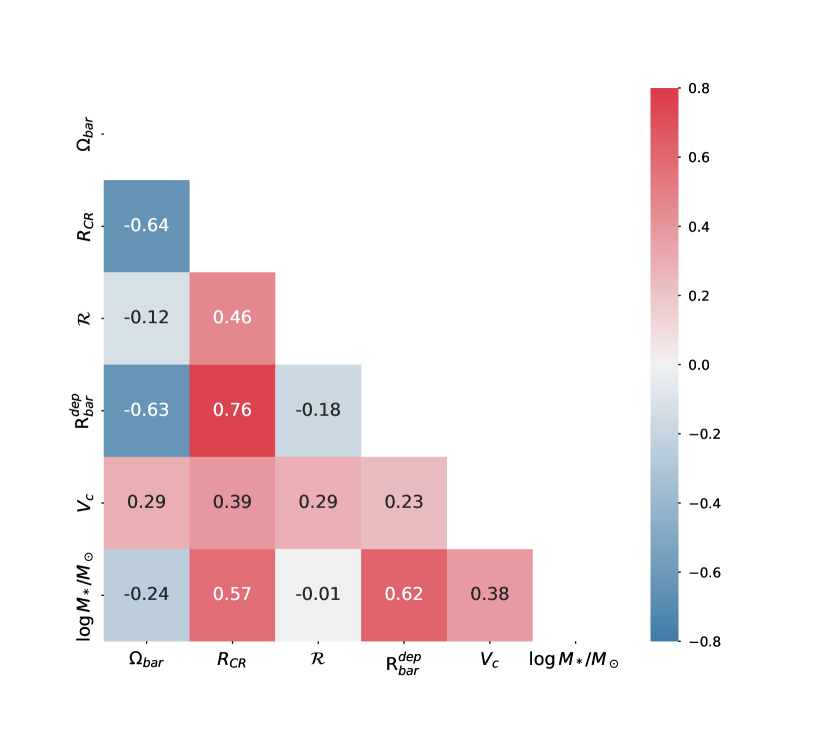
Figure 17: Spearman correlation matrix of quantities shown in Figures 15 and 16

In G20 we reported two strong correlations between the molecular gas fraction $f_{g}=M_{gas}/(M_{*}+M_{gas})$ with $\mathcal{R}$ ($r_{s}={0.54}$) and with $\Omega_{bar}$ ($r_{s}={-0.52)}$. In this work, we found that the relation with the rotation rate is still present, but with more scatter ($r_{s}={0.23}$), and that the relation with $\Omega_{bar}$ disappeared ($r_{s}={0.07}$). It is possible that our previous work was affected by low number statistics, or was biased by some outliers. Although weak, the relation with $\mathcal{R}$ does suggest that the gas role in the bar evolution is important and should be explored in more detail.

We also looked for correlations with other global galactic properties derived from the Pipe3D analysis (Sánchez et al., 2018). Most of these relations are weak, and have a lot of scatter, but we mention two that could be of interest: the Sérsic index has a weak anti-correlation with $\Omega_{bar}$ ($r_{s}={-0.20}$), and $\mathcal{R}$ ($r_{s}={-0.17}$). Similarly, the rotation velocity-to-velocity dispersion ratio within 1 effective radius $v/\sigma$ has a weak correlation with $\Omega_{bar}$ ($r_{s}={0.24}$), and $\mathcal{R}$ ($r_{s}={0.12}$). These two pairs of correlations suggest that more concentrated mass distributions (or more pressure supported systems) produce bars that rotate at lower bar pattern speed, but faster in $\mathcal{R}$. Nonetheless, both $n$ and $v/\sigma$ are not corrected for the presence of the bar. A more realistic study would require such corrections (Gadotti, 2008; Weinzirl et al., 2009; Graham & Li, 2009).

6.3 Where are the ultra-fast bars?

In recent years, the abundance of fast-rotating bars has attracted attention from the cosmological simulations community. The angular momentum exchange in simulations produces high rates of bar slowdown. Roshan et al. (2021b) found mean values for $\mathcal{R}$ range between 2.5 to 3 in the cosmological simulations IllustrinsTNG and EAGLE. Fragkoudi et al. (2021) showed that galaxies more baryon-dominated can remain fast down to z=0. Moreover, Frankel et al. (2022) showed that simulated bars are shorter rather than slower compared to their observed counterparts. Alternatively, Roshan et al. (2021a) showed that bars remain fast in modified gravity theories.

Our sample has a strong component of ultra-fast bars (using the probability distributions, they account for $\sim 20\%$ of our sample). Before attempting to explain their physical origin, we explore other possible systematic errors. As mentioned in Section 3, the TW method is susceptible to fictitious signals in galaxies with low and high inclinations. Face-on galaxies have poor kinematic information, while edge-on galaxies do not have positional information. Also, the symmetry of the TW-integrals requires the bar not to be oriented towards the minor or major axis of the disc.

Figure 18 shows the rotation rate versus the disc photometric inclination. The figure is coloured by the relative orientation of the disc and the bar, highlighting in red galaxies where the relative orientation could be problematic. In particular, we noticed a cluster of ultra-fast bars in the low inclination region (green circle).

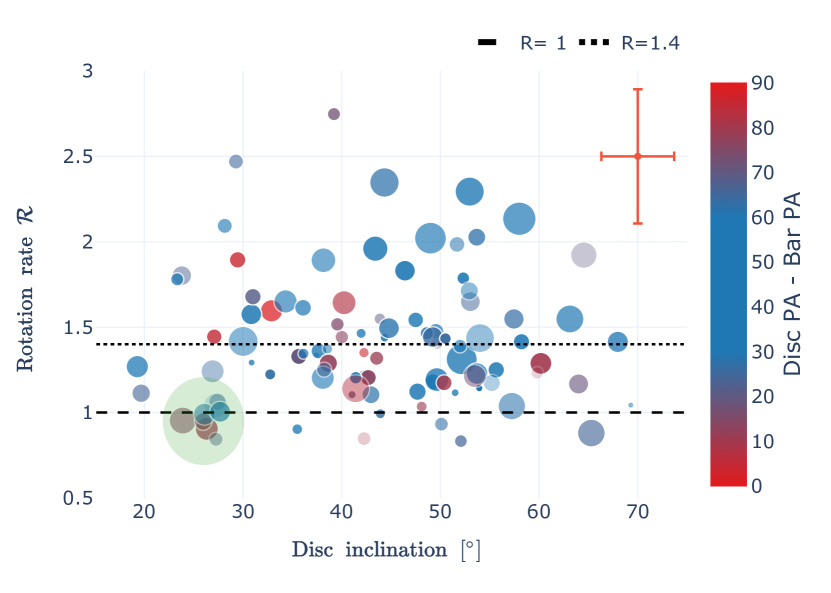
Figure 18: Rotation rate $\mathcal{R}$ versus disc photometric inclination coloured by the relative orientation between the disc and the bar. A cluster of ultra-fast bars is found in the low-inclination region, which we highlight with a green circle.

We create a “quality” sub-sample by introducing the following constrains: inclination within $30\degree<i<60\degree$ and relative orientation $20\degree<|PA_{disc}-PA_{bar}|<70\degree$. This quality sub-sample consists of 55 galaxies, this time with only 6 ultra-fast bars ($\sim 10\%$ of the sample). In other words, 14 of our ultra-fast galaxies were probably the result of systematic errors related to the geometric limitations of the TW-method.

Notably, this quality sub-sample also has stronger correlations compared to the complete sample. In table 2 we compare the correlations discussed in Section 6.2 between both samples.

Relation	Complete Sample	Quality sub-sample
(1)	(2)	(3)
$\Omega_{bar}$ - $\log M_{*}/M_{\odot}$	-0.23	-0.46
$\Omega_{bar}$ - $R_{bar}^{Dep}$	-0.63	-0.71
$\log M_{*}/M_{\odot}$ - $R_{bar}^{Dep}$	0.58	0.69
$\Omega_{bar}$ - $R_{cr}$	-0.64	-0.75
$\Omega_{bar}$ - $V_{c}$	0.29	0.14
$\mathcal{R}$ - $V_{c}$	0.29	0.25
$\Omega_{bar}$ - $n$	-0.20	-0.31
$\mathcal{R}$ - $n$	-0.17	-0.11
$\Omega_{bar}$ - $v/\sigma$	0.24	0.41
$\mathcal{R}$ - $v/\sigma$	0.12	0.06

Table 2: Spearman correlation coefficients in the complete sample and the quality cut sub-sample. Col. (1) Pair of variables. Col. (2) Correlation coefficients in the complete sample Col, (3) Correlation coefficients in the quality sub-sample.

It is possible that some galaxies in our sample have more than one pattern speed (for example from the spiral arms or a nested bar). Although we choose the number of slits to cover only the bar region, we cannot disentangle the effects that other non-axisymmetric structures could have in the estimation of $\mathcal{R}$. Some slow bars in our sample could be affected by the spiral pattern, however it is hard to quantify.

6.4 Milky Way like galaxies

Because of the restrictive nature of the TW method, the selection criteria in our sample was based only upon the morphological type and stellar mass. However, our sample contains galaxies with a great variety of bars sizes, morphological features (rings, spirals), mass distribution (with disc circular velocities that range from 150 to 400 km s^-1) and galactic environments.

To better reflect the parameters of the MW we build a sub-sample making an additional cut in the bar length ($R_{bar}<6$ kpc) and the disc circular velocities ($190<V_{c}<290$ km s^-1). We chose these parameters as they are correlated with $\Omega_{bar}$. We also include the cuts in inclination and relative orientation of the disc-bar discussed in the previous section to improve the overall quality. The resulting MW sub-sample comprises 25 galaxies, that are marked in Table LABEL:tab:master with an asterisk next to the name of the galaxy.

Figure 19 shows the resulting distribution in $\Omega_{bar}$ and $\mathcal{R}$. Most recent estimates of the bar pattern speed in our Galaxy are in the range $\Omega_{bar}\sim 35-45$ km s^-1 kpc^-1, which lies within the 1-sigma upper limit of our distribution.

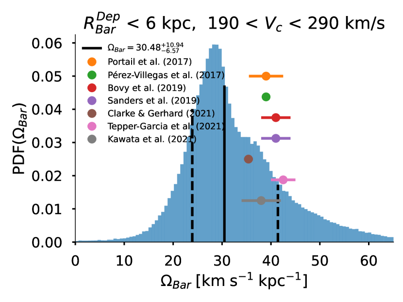
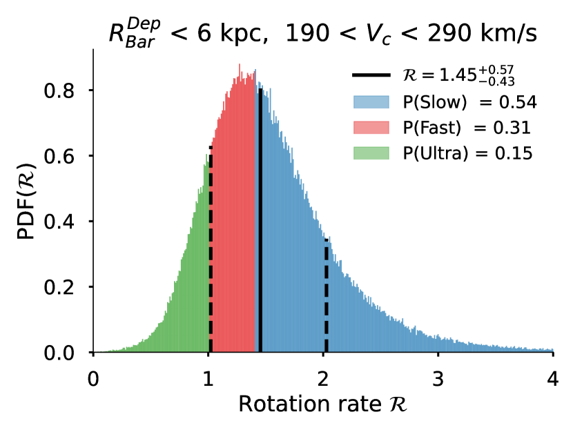
Figure 19: Bar pattern speed and $\mathcal{R}$ distributions of the MW sub-sample. This sub-sample is built by adding cuts in the bar lengths $(R_{bar}^{Dep}<6$kpc) and the disc circular velocity ($190<V_{c}<290$ km s^-1).

7 Discussion

7.1 Improving future measurements

Throughout this work, we have discussed many error sources and biases that appear when measuring the bar pattern speed and derived quantities. The most important of these is the disc PA, where a few degrees of error can change the measurement dramatically. This would not be a problem if different measurements agreed on their uncertainties, but this is usually not the case. In this work, we choose to do an equal weighting of different PA measurements (by increasing their errors artificially until they become consistent), and impose a condition over the linearity of the TW-integrals (see section 5.1). An improvement could be made by using a criterion based on the goodness of fit $\chi^{2}$ (maybe with a threshold condition, or using $\chi^{2}$ to weight the PA), or by modelling the systemic errors of each measurement.

Our procedure is biased towards measurements that produce a linear behaviour in the TW integrals (we are weighting our observations based on the method). Sometimes this includes galaxies that should not work with the TW-method, but nonetheless, produce a measurement that has physical sense (see our discussion in sections 6.3 and 6.4).

We estimated the geometric error of $\Omega_{bar}$ using a MC procedure over the inclination, PA, centre and slits length. However, the number of slits could be an important parameter to consider. In most galaxies the TW integrals follow a linear trend up to near the bar end. We tried to use a number of slits to fill the area enclosed by $R_{\epsilon}$, however, there are exceptions. In some galaxies the linearity can only be seen in the innermost slits, while in others, the central slits are clustered together and only the outermost slits follow a lineal trend. By letting the number of slits be a free parameter (within the uncertainties of the bar radius) the measurements would capture some of this behaviour.

Also important is the bar radius estimation, where morphological features (bulges, rings, ansae, spirals) affect the different measurement techniques. In this work, we choose to model the bar radius using a log-normal distribution with $R_{\epsilon}$ and $R_{PA}$ as the mean and 2-sigma upper limit of the distribution. This could be improved by incorporating other measurements like the the 2-D decomposition model of the surface brightness or the bar maximum torque.

Using hydrodynamical simulations, Hilmi et al. (2020) estimated that observations could be overestimating the bar radius between $\sim 15-55$ per cent, depending on the timescale and orientation of the galactic structures. Cuomo et al. (2021) proposed the maximum torque radius as a better estimator for the bar radius (hereafter $R_{Qb}$). However, this method comes other with important limitations and biases. Most importantly, in various galaxies $R_{Qb}$ does not agree with the visual estimate of what constitutes the bar. Also, the method is affected by the bulge-to-total ratio (B/T) as it can dilute $Q_{b}$ and increase $R_{Qb}$ (Díaz-García et al., 2016a). The B/T ratio also affects the isophote method, but only in exponential weak bars (Lee et al., 2020).

For comparison purposes, we estimated $R_{Qb}$ by de-projecting the r-band DESI image and solving the Poisson equation assuming a constant mass-to-light ratio (Buta & Block, 2001). In Figure 20 we show both bar measuring methods in our sample. We found $R_{Qb}$ to be $\sim 30\%$ smaller than $R_{\epsilon}$ after deprojection.

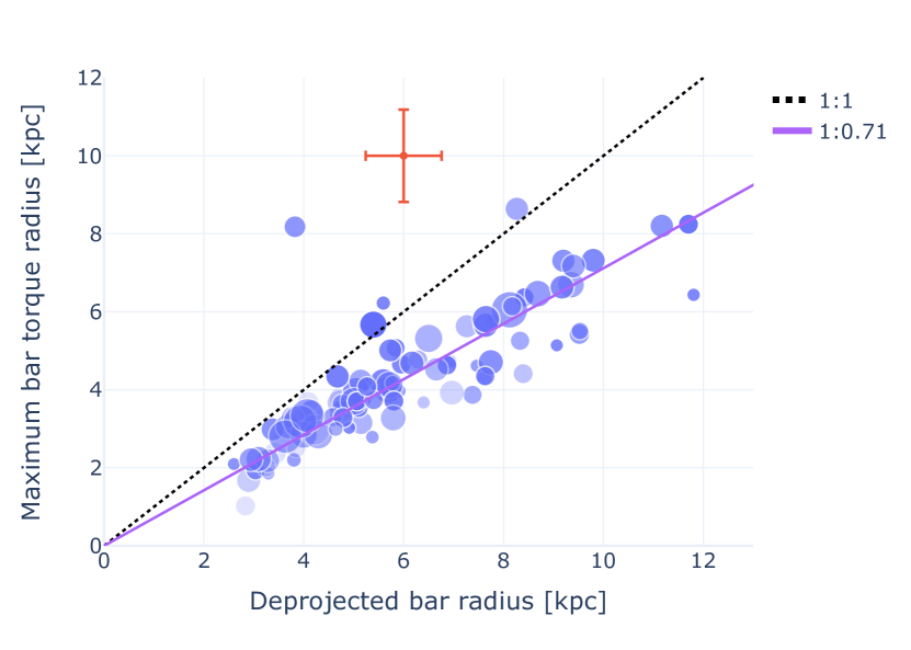
Figure 20: Bar radius estimated using the maximum torque versus the deprojected bar radius estimated from the maximum ellipticity isophote.

We tried using $R_{Qb}$ as the 2-sigma lower limit of the distribution (with $R_{\epsilon}$ as the mean) but in some galaxies, the difference between $R_{\epsilon}$ and $R_{Qb}$ is so significant, that the distribution had a long tail towards high bar radii. We got some reasonable results using both $R_{Qb}$ and $R_{PA}$ as the lower and upper 2-sigma limits, but the distribution of $\mathcal{R}$ of the complete sample widens significantly, including some ultra-fast ($\mathcal{R}$$\sim 1$) and ultra-slow bars ($\mathcal{R}$$\sim 4$). Thus, we choose to use the combination that produced more consistent results. Maybe incorporating a Gaussian Mixture Model to estimate the intrinsic biases could help improve some of these measurements.

8 Conclusions

• We have measured the bar pattern speed, bar radius, corotation radius and rotation rate of a sample of 97 MaNGA galaxies using the TW method. The sample was constructed to resemble the Milky-Way by using cuts in the stellar mass and the morphological type. The TW integrals were computed over the stellar component.

• We used 3 independent measurements of the disc PA from different sources: isophote fitting of the surface brightness, symmetrization of the stellar velocity field and fitting a kinematic model to the H_α velocity field. We assume all measurements are biased and increased their errors to produce an equal weighted PA. We penalise PAs when the TW integrals are not linear.

• We used a MC procedure to estimate the $\Omega_{bar}$ distribution by sampling the PA, inclination, centre and slit length. This procedure let us disentangle the effects of each error source.

• We used the rotation curve from the kinematic bi-symmetric model of H_α velocity field· The model fits non-circular motions produced by the bar, and does not require an asymmetric drift correction.

• Two measurements of the bar radius were obtained from the isophotal procedure $R_{\epsilon}$ and $R_{PA}$. We choose to model the bar radius with a log-normal distribution using these measurements as parameters (mean and 2-sigma).

• We found two significant correlations within our sample: (i) $\Omega_{bar}$-$R_{bar}^{Dep}$-$\log M_{*}/M_{\odot}$ which relates the size of the system to the rotation frequency and (ii) $\Omega_{bar}$-$V_{c}$-$\mathcal{R}$, that suggest fast rotating discs tend to host high pattern speed bars, but slow in rotation rate $\mathcal{R}$.

• We also looked for correlations with various global galactic properties. We found a weak correlation between $\mathcal{R}$ and the gas fraction. Also, the weak relations between $\Omega_{bar}$ and $\mathcal{R}$ with the Sérsic index and $v/\sigma$ ratio within 1 effective radius, suggest that more concentrated mass distributions produce bars that rotate at lower pattern speeds, but faster in $\mathcal{R}$.

• We identify the inclination angle and the relative orientation of the disc-bar as possible sources of ultra-fast rotating bars in our sample. Using a cut in both parameters reduced the frequency of ultra-fast from 20% to 10% of the sample.

• We build a sub-sample of MW galaxies using these quality cuts, and an additional cut in the bar radius and disc circular velocity. The most recent measurements of the MW bar pattern speed lie within the upper 1-sigma of our distribution.

• We suggest future measurements to take into account all possible biases in the procedure or, if possible, model these biases.

Data availability

All Figures and relevant tables are available in the public repository https://github.com/lgarma/MWA_pattern_speed. Other data that support the findings of this study are available from the corresponding author, upon reasonable request.

Appendix A Table

Table 3: Col. (1): Galaxy MaNGA name. Col. (2): Logarithmic Stellar Mass. Col. (3): Weighted Disc Position Angle (PA that are equally weighted, p:photometric, s:symetric, m:model). Col. (4): Bar photometric position angle. Col. (5): Weighted disc inclination (photometric + model). Col. (6): Disc circular velocity fitted from equation 7 with $\gamma=1$. Col. (7): Bar radius estimated from the maximum isophote ellipticity method. Col. (8): Deprojected bar radius. Col. (9): Bar pattern speed. Col. (10): Corotation radius. Col. (11): Rotation rate.

Galaxy	$\log(M/M_{\odot})$	Disc PA (weighted)	Bar PA	$i$	$V_{c}$	$R_{bar}$	$R_{bar}^{Dep}$	$\Omega_{bar}$	$R_{cr}$	$\mathcal{R}$
		[$\degree$]	[$\degree$]	[$\degree$]	[km s-1]	[arcsec]	[kpc]	[km s-1 kpc-1]	[kpc]
(1)	(2)	(3)	(4)	(5)	(6)	(7)	(8)	(9)	(10)	(11)
7495-12704*	$10.8$	$172.8\pm 1.1$ (s+m)	$147.8\pm 3.5$	$55.4^{+2.5}_{-2.6}$	$223.1\pm 1.2$	$5.1\pm 2.0$	$3.9^{+1.3}_{-1.0}$	$26.9^{+4.1}_{-5.0}$	$7.6^{+2.1}_{-1.3}$	$2.0^{+0.9}_{-0.6}$
7958-6101	$10.5$	$153.9\pm 0.7$ (p+s+m)	$158.6\pm 0.9$	$40.7^{+1.1}_{-1.2}$	$182.3\pm 1.1$	$5.2\pm 0.3$	$2.6^{+0.1}_{-0.1}$	$47.9^{+13.1}_{-16.5}$	$3.5^{+1.5}_{-0.9}$	$1.4^{+0.6}_{-0.4}$
7958-3702	$10.7$	$144.9\pm 1.0$ (p+s)	$68.2\pm 4.2$	$50.0^{+2.5}_{-2.6}$	$246.8\pm 1.7$	$2.3\pm 0.2$	$2.8^{+0.3}_{-0.3}$	$74.3^{+11.2}_{-11.8}$	$3.3^{+0.6}_{-0.5}$	$1.2^{+0.3}_{-0.2}$
7977-9102	$10.8$	$113.0\pm 1.0$ (m)	$138.2\pm 2.5$	$49.1^{+3.2}_{-3.4}$	$311.9\pm 1.5$	$2.3\pm 0.5$	$3.7^{+0.8}_{-0.6}$	$41.1^{+5.2}_{-5.5}$	$7.4^{+1.2}_{-0.9}$	$2.0^{+0.5}_{-0.4}$
7993-12704	$11.2$	$127.6\pm 1.5$ (p+s)	$26.2\pm 2.2$	$30.7^{+3.0}_{-3.3}$	$252.7\pm 5.5$	$11.1\pm 1.8$	$11.2^{+1.7}_{-1.6}$	$24.1^{+6.9}_{-6.2}$	$10.6^{+3.5}_{-2.4}$	$0.9^{+0.4}_{-0.2}$
8078-12703	$10.9$	$4.5\pm 0.9$ (p+s)	$68.0\pm 1.1$	$38.5^{+3.2}_{-3.4}$	$294.3\pm 2.5$	$8.2\pm 0.9$	$5.9^{+0.6}_{-0.6}$	$42.6^{+8.5}_{-8.0}$	$6.5^{+1.8}_{-1.4}$	$1.1^{+0.3}_{-0.3}$
8085-3704	$10.7$	$104.0\pm 3.0$ (s)	$108.1\pm 3.0$	$31.8^{+7.0}_{-8.8}$	$196.4\pm 12.6$	$5.1\pm 1.2$	$4.0^{+0.8}_{-0.7}$	$34.8^{+10.8}_{-8.0}$	$4.5^{+1.8}_{-1.4}$	$1.1^{+0.5}_{-0.4}$
8088-3701*	$10.5$	$44.0\pm 2.0$ (s)	$169.8\pm 3.1$	$30.3^{+5.7}_{-6.9}$	$244.7\pm 3.0$	$4.0\pm 0.7$	$4.2^{+0.6}_{-0.6}$	$31.4^{+13.4}_{-10.7}$	$7.9^{+2.6}_{-1.9}$	$1.9^{+0.7}_{-0.5}$
8091-6101	$11.2$	$85.8\pm 0.6$ (p+s+m)	$42.8\pm 2.7$	$46.1^{+1.8}_{-1.9}$	$259.3\pm 3.2$	$7.3\pm 0.8$	$7.6^{+0.8}_{-0.7}$	$23.3^{+2.6}_{-3.0}$	$11.1^{+1.6}_{-1.2}$	$1.5^{+0.3}_{-0.2}$
8091-12701	$10.8$	$162.1\pm 0.8$ (s+m)	$111.0\pm 0.4$	$37.6^{+4.2}_{-4.7}$	$224.7\pm 11.9$	$8.2\pm 0.9$	$11.7^{+1.2}_{-1.2}$	$11.8^{+1.7}_{-1.5}$	$18.4^{+2.9}_{-2.4}$	$1.6^{+0.3}_{-0.3}$
8135-6103	$11.0$	$34.9\pm 2.4$ (m)	$8.3\pm 2.2$	$37.4^{+0.5}_{-0.5}$	$239.8\pm 4.4$	$7.5\pm 1.2$	$8.3^{+1.2}_{-1.1}$	$20.2^{+4.1}_{-5.1}$	$11.0^{+3.0}_{-2.0}$	$1.3^{+0.4}_{-0.3}$
8146-9102	$10.6$	$17.0\pm 1.0$ (s)	$157.4\pm 4.2$	$54.4^{+2.7}_{-2.8}$	$209.5\pm 2.4$	$3.9\pm 0.6$	$6.2^{+1.0}_{-0.9}$	$23.1^{+1.8}_{-1.7}$	$8.7^{+0.5}_{-0.4}$	$1.4^{+0.2}_{-0.2}$
8241-6102	$10.6$	$117.0\pm 1.5$ (s)	$174.3\pm 5.3$	$21.0^{+1.7}_{-1.8}$	$297.6\pm 2.3$	$4.0\pm 0.2$	$3.3^{+0.2}_{-0.2}$	$45.2^{+10.1}_{-8.5}$	$5.9^{+1.3}_{-1.3}$	$1.8^{+0.4}_{-0.4}$
8245-12702	$11.1$	$17.7\pm 0.7$ (p+s)	$170.3\pm 3.8$	$51.8^{+2.7}_{-2.8}$	$351.2\pm 3.5$	$10.8\pm 1.8$	$9.4^{+1.5}_{-1.3}$	$26.3^{+1.9}_{-2.8}$	$11.6^{+1.0}_{-0.7}$	$1.3^{+0.2}_{-0.2}$
8257-6103	$11.2$	$135.9\pm 0.9$ (s+m)	$54.6\pm 4.4$	$25.8^{+2.6}_{-2.9}$	$426.1\pm 5.9$	$4.2\pm 0.4$	$6.3^{+0.6}_{-0.6}$	$32.1^{+7.0}_{-5.9}$	$11.9^{+2.2}_{-2.1}$	$1.9^{+0.4}_{-0.4}$
8312-12702*	$10.6$	$92.5\pm 1.4$ (p+s)	$123.6\pm 2.5$	$38.9^{+4.2}_{-4.7}$	$230.2\pm 1.1$	$6.8\pm 1.6$	$5.0^{+1.0}_{-0.9}$	$29.2^{+4.1}_{-3.3}$	$7.5^{+0.8}_{-0.8}$	$1.5^{+0.3}_{-0.3}$
8312-12705	$10.5$	$92.4\pm 5.6$ (m)	$130.8\pm 6.5$	$36.7^{+5.6}_{-6.4}$	$108.2\pm 11.9$	$7.4\pm 1.7$	$5.4^{+1.1}_{-1.0}$	$14.7^{+6.3}_{-5.1}$	$5.6^{+4.8}_{-2.8}$	$1.0^{+0.9}_{-0.5}$
8319-12704	$10.7$	$109.2\pm 1.0$ (p)	$146.0\pm 1.9$	$42.8^{+1.6}_{-1.6}$	$176.9\pm 1.2$	$6.8\pm 0.7$	$4.8^{+0.5}_{-0.4}$	$30.9^{+2.5}_{-2.3}$	$5.7^{+0.4}_{-0.4}$	$1.2^{+0.1}_{-0.1}$
8320-6101*	$10.4$	$4.1\pm 1.0$ (p+s)	$60.2\pm 7.0$	$47.4^{+2.0}_{-2.0}$	$203.2\pm 12.2$	$4.2\pm 0.7$	$3.3^{+0.5}_{-0.4}$	$54.1^{+9.8}_{-10.5}$	$3.1^{+1.0}_{-0.9}$	$0.9^{+0.3}_{-0.3}$
8324-12702*	$11.0$	$68.5\pm 0.8$ (p+m)	$23.9\pm 7.5$	$35.9^{+1.2}_{-1.3}$	$252.4\pm 1.1$	$7.5\pm 0.4$	$5.4^{+0.3}_{-0.3}$	$33.3^{+7.0}_{-7.4}$	$7.2^{+2.1}_{-1.5}$	$1.3^{+0.4}_{-0.3}$
8341-12704	$10.7$	$55.5\pm 1.9$ (p+m)	$80.9\pm 1.2$	$25.2^{+3.3}_{-3.7}$	$116.7\pm 1.4$	$7.5\pm 0.4$	$4.9^{+0.2}_{-0.2}$	$18.5^{+4.6}_{-4.1}$	$5.4^{+1.8}_{-1.6}$	$1.1^{+0.4}_{-0.3}$
8444-12703*	$10.9$	$4.9\pm 0.6$ (s+m)	$31.7\pm 9.5$	$37.2^{+1.2}_{-1.2}$	$237.7\pm 1.3$	$5.7\pm 0.9$	$5.0^{+0.7}_{-0.7}$	$40.9^{+4.0}_{-3.9}$	$4.5^{+0.8}_{-0.8}$	$0.9^{+0.2}_{-0.2}$
8450-9102*	$10.4$	$14.7\pm 1.1$ (p+s+m)	$-6.6\pm 4.4$	$48.6^{+1.4}_{-1.4}$	$199.0\pm 2.2$	$3.9\pm 0.4$	$4.6^{+0.4}_{-0.4}$	$29.5^{+1.7}_{-1.9}$	$6.6^{+0.4}_{-0.4}$	$1.4^{+0.2}_{-0.2}$
8453-12701	$10.4$	$109.0\pm 1.3$ (s)	$45.6\pm 2.8$	$41.6^{+2.3}_{-2.4}$	$149.5\pm 4.0$	$5.6\pm 0.3$	$3.8^{+0.2}_{-0.2}$	$23.4^{+4.5}_{-5.4}$	$4.8^{+2.0}_{-1.5}$	$1.3^{+0.5}_{-0.4}$
8454-12702	$11.0$	$66.0\pm 1.7$ (s)	$93.1\pm 2.8$	$45.4^{+2.7}_{-2.8}$	$250.9\pm 2.5$	$4.4\pm 0.5$	$8.3^{+0.8}_{-0.8}$	$26.1^{+2.1}_{-1.8}$	$9.9^{+0.7}_{-1.0}$	$1.2^{+0.2}_{-0.2}$
8465-12705	$10.9$	$49.3\pm 0.7$ (s+m)	$34.9\pm 4.5$	$53.5^{+4.8}_{-5.1}$	$290.6\pm 2.1$	$5.6\pm 0.6$	$3.8^{+0.5}_{-0.4}$	$65.7^{+10.2}_{-10.2}$	$4.9^{+0.3}_{-0.3}$	$1.3^{+0.2}_{-0.2}$
8486-6101*	$10.8$	$114.9\pm 1.1$ (s+m)	$77.6\pm 3.0$	$40.4^{+2.8}_{-3.0}$	$192.7\pm 3.9$	$2.9\pm 0.9$	$4.2^{+1.1}_{-0.9}$	$27.5^{+3.0}_{-2.9}$	$6.8^{+0.8}_{-0.7}$	$1.6^{+0.5}_{-0.4}$
8552-9101*	$11.0$	$110.2\pm 0.9$ (s+m)	$135.4\pm 1.7$	$32.7^{+1.3}_{-1.3}$	$203.8\pm 1.7$	$3.9\pm 0.4$	$5.8^{+0.5}_{-0.5}$	$26.7^{+2.7}_{-3.0}$	$7.1^{+0.7}_{-0.6}$	$1.2^{+0.2}_{-0.2}$
8561-3704	$10.4$	$169.2\pm 1.4$ (p+s)	$156.5\pm 3.3$	$39.5^{+2.0}_{-2.0}$	$234.3\pm 23.3$	$5.6\pm 1.3$	$5.7^{+1.1}_{-1.0}$	$27.0^{+3.6}_{-4.8}$	$4.9^{+2.6}_{-2.2}$	$0.8^{+0.5}_{-0.4}$
8589-12705	$11.1$	$167.8\pm 1.3$ (p+m)	$34.7\pm 2.7$	$25.0^{+2.3}_{-2.5}$	$309.2\pm 1.3$	$7.4\pm 1.2$	$4.8^{+0.7}_{-0.7}$	$28.9^{+9.1}_{-8.8}$	$10.1^{+3.4}_{-2.3}$	$2.1^{+0.8}_{-0.5}$
8596-12704	$10.9$	$82.6\pm 1.8$ (p+m)	$58.4\pm 1.9$	$45.0^{+3.0}_{-3.2}$	$258.2\pm 1.5$	$7.6\pm 1.3$	$6.7^{+1.0}_{-0.9}$	$25.6^{+4.4}_{-4.7}$	$9.5^{+1.8}_{-1.4}$	$1.4^{+0.3}_{-0.3}$
8597-12703*	$10.8$	$170.4\pm 1.9$ (p+s+m)	$137.3\pm 1.6$	$42.6^{+1.1}_{-1.1}$	$228.2\pm 0.9$	$8.2\pm 0.9$	$5.1^{+0.5}_{-0.5}$	$28.4^{+5.5}_{-6.8}$	$7.4^{+1.9}_{-1.2}$	$1.5^{+0.4}_{-0.3}$
8602-3701	$10.3$	$153.1\pm 0.7$ (p+s)	$186.3\pm 3.6$	$50.0^{+1.6}_{-1.7}$	$175.4\pm 3.1$	$4.0\pm 0.4$	$3.2^{+0.3}_{-0.3}$	$26.9^{+2.9}_{-3.5}$	$5.8^{+0.7}_{-0.6}$	$1.8^{+0.3}_{-0.3}$
8602-12701	$11.3$	$156.2\pm 2.2$ (p)	$193.7\pm 0.7$	$39.8^{+1.8}_{-1.9}$	$256.7\pm 7.3$	$12.3\pm 0.6$	$7.8^{+0.4}_{-0.4}$	$24.7^{+6.8}_{-8.0}$	$9.4^{+4.3}_{-2.6}$	$1.2^{+0.5}_{-0.3}$
8602-12705	$11.2$	$143.5\pm 1.5$ (m)	$185.5\pm 0.7$	$37.9^{+2.5}_{-2.6}$	$184.4\pm 4.7$	$11.1\pm 1.2$	$8.4^{+0.8}_{-0.8}$	$15.9^{+3.1}_{-2.8}$	$11.4^{+2.5}_{-1.9}$	$1.4^{+0.3}_{-0.3}$
8612-12702	$11.2$	$47.8\pm 2.1$ (p+s)	$69.5\pm 2.5$	$47.5^{+3.9}_{-4.2}$	$287.8\pm 0.7$	$5.1\pm 0.3$	$7.6^{+0.5}_{-0.4}$	$20.6^{+5.8}_{-6.7}$	$12.6^{+5.5}_{-3.9}$	$1.6^{+0.7}_{-0.5}$
8615-3701	$10.8$	$106.7\pm 1.7$ (s+m)	$72.2\pm 3.4$	$33.8^{+4.6}_{-5.2}$	$137.9\pm 3.5$	$2.5\pm 1.0$	$3.6^{+1.2}_{-0.9}$	$29.7^{+5.5}_{-4.3}$	$3.7^{+0.9}_{-0.9}$	$1.0^{+0.4}_{-0.3}$
8616-6104	$10.7$	$32.0\pm 0.7$ (p+s)	$-0.6\pm 6.4$	$61.6^{+4.5}_{-4.7}$	$251.7\pm 6.7$	$3.9\pm 0.4$	$7.0^{+1.3}_{-1.0}$	$24.1^{+3.4}_{-4.1}$	$9.8^{+1.9}_{-1.5}$	$1.4^{+0.4}_{-0.3}$
8622-12704	$11.1$	$76.6\pm 1.3$ (p+m)	$62.8\pm 0.2$	$42.8^{+1.9}_{-1.9}$	$265.3\pm 4.8$	$3.8\pm 0.2$	$5.9^{+0.3}_{-0.3}$	$27.3^{+6.3}_{-8.9}$	$8.5^{+3.6}_{-2.0}$	$1.4^{+0.6}_{-0.3}$
8624-9102	$10.6$	$142.0\pm 1.3$ (s)	$132.4\pm 1.9$	$46.6^{+2.0}_{-2.1}$	$198.4\pm 3.5$	$8.9\pm 0.9$	$5.4^{+0.5}_{-0.5}$	$25.3^{+5.1}_{-6.8}$	$7.1^{+1.8}_{-1.1}$	$1.3^{+0.4}_{-0.2}$
8625-12703	$11.0$	$88.0\pm 1.0$ (s)	$129.2\pm 5.8$	$69.1^{+0.4}_{-0.4}$	$266.8\pm 3.7$	$5.0\pm 0.5$	$7.4^{+0.7}_{-0.7}$	$27.6^{+6.3}_{-8.3}$	$7.7^{+3.5}_{-1.9}$	$1.0^{+0.5}_{-0.3}$
8655-3701	$11.0$	$148.0\pm 1.7$ (s)	$160.0\pm 2.0$	$36.0^{+6.7}_{-8.1}$	$140.8\pm 3.2$	$5.9\pm 1.0$	$9.2^{+1.4}_{-1.2}$	$15.4^{+5.2}_{-4.9}$	$8.7^{+3.4}_{-2.4}$	$1.0^{+0.4}_{-0.3}$
8656-6103*	$11.2$	$14.6\pm 1.6$ (s+m)	$-39.6\pm 2.6$	$27.4^{+5.0}_{-6.1}$	$254.3\pm 3.7$	$3.3\pm 0.6$	$4.8^{+0.7}_{-0.6}$	$32.7^{+11.0}_{-8.6}$	$7.9^{+2.5}_{-1.8}$	$1.7^{+0.6}_{-0.4}$
8713-9102	$10.6$	$151.5\pm 1.1$ (s+m)	$187.7\pm 3.1$	$34.6^{+4.2}_{-4.7}$	$131.9\pm 26.2$	$6.8\pm 0.7$	$5.3^{+0.5}_{-0.5}$	$21.1^{+4.0}_{-3.3}$	$5.3^{+1.6}_{-1.3}$	$1.0^{+0.3}_{-0.3}$
8715-12701*	$10.9$	$134.0\pm 1.3$ (s)	$166.5\pm 1.6$	$40.2^{+1.1}_{-1.1}$	$257.7\pm 4.2$	$10.3\pm 1.7$	$5.7^{+0.8}_{-0.8}$	$25.7^{+3.8}_{-5.4}$	$7.8^{+3.4}_{-1.9}$	$1.4^{+0.6}_{-0.4}$
8718-12701	$10.7$	$72.1\pm 2.4$ (m)	$88.2\pm 0.8$	$37.0^{+1.9}_{-1.9}$	$132.3\pm 3.3$	$7.5\pm 0.8$	$8.2^{+0.8}_{-0.7}$	$10.0^{+1.6}_{-2.2}$	$12.3^{+3.6}_{-2.0}$	$1.5^{+0.5}_{-0.3}$
8721-6103	$11.2$	$50.8\pm 0.8$ (s+m)	$136.3\pm 3.0$	$32.7^{+5.4}_{-6.4}$	$352.8\pm 3.5$	$4.5\pm 0.7$	$5.1^{+0.8}_{-0.7}$	$40.6^{+13.1}_{-9.3}$	$8.5^{+2.3}_{-2.2}$	$1.6^{+0.5}_{-0.5}$
8938-12702	$11.1$	$53.4\pm 1.4$ (s+m)	$32.1\pm 0.3$	$43.9^{+1.4}_{-1.4}$	$303.4\pm 2.5$	$7.6\pm 0.4$	$6.9^{+0.3}_{-0.3}$	$25.9^{+8.2}_{-9.2}$	$10.8^{+5.2}_{-3.3}$	$1.5^{+0.7}_{-0.5}$
8940-12702*	$11.0$	$140.2\pm 0.9$ (p+m)	$112.2\pm 1.3$	$44.7^{+1.0}_{-1.1}$	$240.1\pm 3.2$	$8.9\pm 2.1$	$5.7^{+1.1}_{-1.0}$	$36.7^{+2.2}_{-2.4}$	$5.7^{+0.4}_{-0.4}$	$1.0^{+0.2}_{-0.2}$
8948-12702	$11.0$	$1.0\pm 1.3$ (s)	$49.7\pm 0.6$	$19.8^{+1.1}_{-1.2}$	$246.5\pm 5.7$	$6.0\pm 1.0$	$3.4^{+0.5}_{-0.5}$	$46.5^{+28.5}_{-21.1}$	$4.1^{+1.2}_{-0.5}$	$1.3^{+0.4}_{-0.3}$
8978-9101*	$10.7$	$93.6\pm 0.7$ (s+m)	$251.5\pm 0.8$	$35.1^{+2.7}_{-2.9}$	$202.1\pm 2.3$	$5.8\pm 0.6$	$3.8^{+0.4}_{-0.3}$	$26.6^{+3.6}_{-4.0}$	$6.4^{+1.2}_{-0.9}$	$1.7^{+0.4}_{-0.3}$
8978-3701	$10.4$	$19.6\pm 1.4$ (p+s)	$126.0\pm 0.5$	$46.4^{+5.1}_{-5.6}$	$245.1\pm 47.7$	$5.6\pm 0.3$	$4.8^{+0.5}_{-0.5}$	$32.6^{+13.0}_{-11.2}$	$5.8^{+2.3}_{-1.9}$	$1.2^{+0.5}_{-0.4}$
8979-12701	$11.2$	$121.0\pm 1.1$ (s+m)	$161.9\pm 4.4$	$50.6^{+0.7}_{-0.7}$	$286.5\pm 1.2$	$4.2\pm 1.0$	$9.3^{+1.9}_{-1.6}$	$24.7^{+2.8}_{-2.5}$	$10.4^{+1.3}_{-1.3}$	$1.1^{+0.3}_{-0.2}$
8983-12701*	$10.5$	$70.4\pm 0.8$ (p+s+m)	$125.1\pm 8.7$	$51.6^{+4.1}_{-4.4}$	$245.6\pm 7.4$	$3.8\pm 0.6$	$3.1^{+0.6}_{-0.5}$	$46.6^{+9.0}_{-9.2}$	$4.8^{+1.0}_{-1.0}$	$1.5^{+0.4}_{-0.4}$
8983-3703*	$10.8$	$174.9\pm 0.6$ (p+s+m)	$147.3\pm 3.5$	$57.9^{+3.3}_{-3.5}$	$205.1\pm 2.7$	$4.9\pm 1.9$	$4.1^{+1.3}_{-1.1}$	$29.2^{+4.9}_{-6.6}$	$6.9^{+2.0}_{-1.5}$	$1.7^{+0.8}_{-0.5}$
8984-12704*	$10.4$	$114.0\pm 1.7$ (s)	$73.7\pm 0.8$	$35.1^{+6.0}_{-7.1}$	$255.3\pm 5.0$	$9.3\pm 1.0$	$5.8^{+0.6}_{-0.6}$	$21.3^{+5.2}_{-4.0}$	$11.4^{+1.9}_{-1.6}$	$2.0^{+0.4}_{-0.3}$
8985-9102	$11.0$	$127.0\pm 1.7$ (m)	$45.4\pm 3.4$	$57.5^{+1.6}_{-1.6}$	$295.0\pm 7.6$	$3.2\pm 0.3$	$8.4^{+0.9}_{-0.8}$	$23.1^{+5.5}_{-9.1}$	$10.3^{+7.2}_{-4.2}$	$1.2^{+0.9}_{-0.5}$
8989-3703	$10.6$	$36.1\pm 0.9$ (s+m)	$47.3\pm 0.5$	$46.3^{+1.2}_{-1.3}$	$363.2\pm 20.4$	$8.2\pm 1.4$	$4.7^{+0.7}_{-0.6}$	$46.3^{+4.7}_{-5.4}$	$4.8^{+1.5}_{-1.2}$	$1.0^{+0.4}_{-0.3}$
8993-12701	$11.1$	$138.0\pm 0.9$ (s+m)	$70.6\pm 1.4$	$54.9^{+7.4}_{-8.2}$	$307.3\pm 1.1$	$8.3\pm 0.9$	$6.5^{+1.6}_{-1.1}$	$53.0^{+14.3}_{-15.5}$	$5.7^{+1.5}_{-0.9}$	$0.9^{+0.3}_{-0.2}$
9025-3703	$11.1$	$52.0\pm 0.7$ (s+m)	$163.1\pm 2.2$	$32.6^{+2.6}_{-2.8}$	$303.5\pm 17.6$	$4.3\pm 0.2$	$5.6^{+0.3}_{-0.3}$	$32.2^{+3.3}_{-3.0}$	$7.5^{+0.6}_{-0.8}$	$1.3^{+0.1}_{-0.1}$
9028-12704*	$10.7$	$55.6\pm 0.9$ (p+s+m)	$1.2\pm 0.3$	$49.3^{+1.9}_{-2.0}$	$239.9\pm 0.9$	$4.7\pm 0.2$	$4.6^{+0.3}_{-0.3}$	$35.7^{+10.2}_{-9.7}$	$6.5^{+2.3}_{-1.6}$	$1.4^{+0.5}_{-0.3}$
9029-12704*	$10.8$	$116.0\pm 1.0$ (s)	$85.0\pm 2.0$	$51.2^{+2.5}_{-2.6}$	$227.6\pm 0.8$	$6.3\pm 1.0$	$5.1^{+0.8}_{-0.7}$	$27.7^{+3.2}_{-3.6}$	$8.0^{+1.1}_{-1.1}$	$1.5^{+0.3}_{-0.3}$
9042-12703	$10.8$	$147.0\pm 1.1$ (s+m)	$105.5\pm 2.4$	$40.1^{+8.8}_{-10.8}$	$334.6\pm 12.8$	$8.6\pm 0.4$	$6.9^{+0.8}_{-0.6}$	$36.9^{+10.0}_{-5.8}$	$9.1^{+1.9}_{-1.7}$	$1.3^{+0.3}_{-0.3}$
9046-12702*	$10.9$	$41.1\pm 1.2$ (p+s+m)	$89.5\pm 1.7$	$43.2^{+0.8}_{-0.8}$	$245.2\pm 1.5$	$6.1\pm 0.6$	$5.1^{+0.5}_{-0.5}$	$31.0^{+3.8}_{-4.0}$	$7.4^{+0.8}_{-1.1}$	$1.4^{+0.2}_{-0.2}$
9047-12703	$11.3$	$104.7\pm 0.7$ (p+s)	$133.9\pm 1.6$	$54.1^{+0.6}_{-0.6}$	$310.9\pm 2.5$	$9.3\pm 0.5$	$11.8^{+0.6}_{-0.6}$	$21.5^{+1.6}_{-1.8}$	$13.5^{+1.2}_{-0.9}$	$1.1^{+0.1}_{-0.1}$
9182-12703	$11.1$	$121.5\pm 0.9$ (s+m)	$133.4\pm 1.4$	$31.5^{+5.0}_{-5.8}$	$278.0\pm 3.1$	$5.8\pm 1.3$	$8.7^{+1.8}_{-1.5}$	$32.0^{+6.5}_{-4.5}$	$7.8^{+1.8}_{-1.2}$	$0.9^{+0.3}_{-0.2}$
9187-3701	$11.2$	$143.9\pm 2.1$ (s+m)	$99.9\pm 0.5$	$42.0^{+5.5}_{-6.2}$	$105.2\pm 1.5$	$5.3\pm 0.3$	$9.5^{+0.8}_{-0.7}$	$8.2^{+2.3}_{-1.9}$	$11.4^{+2.5}_{-2.1}$	$1.2^{+0.3}_{-0.2}$
9187-12704	$10.9$	$78.2\pm 0.9$ (s+m)	$93.7\pm 1.7$	$42.0^{+1.8}_{-1.8}$	$214.5\pm 1.3$	$8.4\pm 0.9$	$5.2^{+0.5}_{-0.5}$	$12.4^{+3.5}_{-3.7}$	$14.3^{+3.7}_{-2.7}$	$2.7^{+0.8}_{-0.5}$
9196-12701	$11.0$	$123.9\pm 2.2$ (s+m)	$178.7\pm 0.7$	$29.9^{+0.5}_{-0.5}$	$305.9\pm 1.1$	$12.6\pm 0.6$	$9.1^{+0.4}_{-0.4}$	$23.8^{+6.9}_{-7.0}$	$11.7^{+3.2}_{-2.2}$	$1.3^{+0.4}_{-0.3}$
9484-12703	$10.7$	$118.0\pm 1.7$ (s)	$101.5\pm 5.9$	$27.4^{+2.0}_{-2.1}$	$277.4\pm 5.8$	$9.5\pm 0.5$	$6.4^{+0.3}_{-0.3}$	$32.6^{+5.5}_{-5.7}$	$5.4^{+2.5}_{-2.1}$	$0.8^{+0.4}_{-0.3}$
9490-6102	$10.4$	$165.4\pm 1.0$ (p)	$149.5\pm 3.0$	$58.3^{+4.1}_{-4.3}$	$212.1\pm 4.2$	$8.0\pm 1.3$	$5.8^{+1.1}_{-0.9}$	$27.9^{+4.9}_{-6.5}$	$6.7^{+2.2}_{-1.3}$	$1.2^{+0.5}_{-0.3}$
9492-6101	$10.4$	$6.0\pm 1.5$ (s)	$158.4\pm 1.9$	$35.5^{+5.1}_{-5.8}$	$138.6\pm 4.4$	$4.6\pm 0.8$	$2.9^{+0.4}_{-0.4}$	$24.9^{+5.2}_{-4.4}$	$3.7^{+1.5}_{-1.4}$	$1.2^{+0.6}_{-0.5}$
9502-12703*	$11.2$	$22.0\pm 1.3$ (s)	$166.1\pm 3.3$	$42.0^{+7.9}_{-9.4}$	$245.2\pm 2.3$	$4.9\pm 0.5$	$3.4^{+0.5}_{-0.4}$	$29.3^{+7.7}_{-5.6}$	$7.9^{+1.5}_{-1.4}$	$2.3^{+0.5}_{-0.5}$
9867-12704*	$10.5$	$90.1\pm 1.6$ (p+s)	$56.2\pm 2.7$	$51.0^{+3.0}_{-3.1}$	$202.5\pm 1.8$	$3.5\pm 0.6$	$2.9^{+0.5}_{-0.4}$	$43.5^{+6.4}_{-5.9}$	$3.4^{+1.6}_{-1.6}$	$1.2^{+0.6}_{-0.5}$
9881-12705	$10.8$	$49.2\pm 1.3$ (p+s+m)	$62.3\pm 0.9$	$36.0^{+3.3}_{-3.6}$	$225.4\pm 3.6$	$11.4\pm 0.6$	$7.5^{+0.3}_{-0.4}$	$22.2^{+2.9}_{-3.0}$	$9.6^{+1.5}_{-1.2}$	$1.3^{+0.2}_{-0.2}$
9890-12702	$11.2$	$139.3\pm 0.7$ (s+m)	$121.6\pm 1.8$	$42.2^{+0.7}_{-0.7}$	$240.6\pm 0.9$	$5.3\pm 1.2$	$7.7^{+1.5}_{-1.3}$	$27.0^{+1.8}_{-2.0}$	$8.5^{+0.8}_{-0.7}$	$1.1^{+0.2}_{-0.2}$
9894-12702	$10.7$	$6.9\pm 1.1$ (p+s)	$142.3\pm 3.1$	$43.9^{+10.2}_{-12.6}$	$421.7\pm 35.4$	$3.2\pm 0.3$	$4.7^{+1.0}_{-0.7}$	$39.6^{+10.7}_{-6.2}$	$10.2^{+2.2}_{-2.0}$	$2.1^{+0.6}_{-0.5}$
10001-6102	$10.7$	$55.2\pm 1.1$ (p)	$72.9\pm 2.5$	$55.3^{+7.0}_{-7.7}$	$296.9\pm 27.4$	$6.8\pm 1.6$	$4.3^{+1.0}_{-0.8}$	$38.7^{+6.4}_{-7.0}$	$8.4^{+3.9}_{-3.5}$	$1.9^{+1.0}_{-0.8}$
10213-12705*	$10.7$	$152.2\pm 2.2$ (p+s)	$14.1\pm 1.4$	$40.6^{+4.2}_{-4.6}$	$281.7\pm 4.3$	$7.5\pm 0.4$	$5.8^{+0.4}_{-0.4}$	$24.1^{+4.4}_{-4.4}$	$10.6^{+1.6}_{-1.3}$	$1.8^{+0.3}_{-0.2}$
10222-12704	$11.1$	$148.7\pm 0.7$ (s+m)	$38.7\pm 14.7$	$23.8^{+2.3}_{-2.6}$	$346.4\pm 2.7$	$4.4\pm 0.7$	$7.2^{+1.1}_{-0.9}$	$31.3^{+4.5}_{-3.9}$	$10.5^{+1.6}_{-1.4}$	$1.4^{+0.3}_{-0.3}$
10510-6101	$10.7$	$36.1\pm 2.4$ (p+s)	$73.1\pm 3.4$	$43.2^{+7.8}_{-9.2}$	$314.4\pm 6.4$	$3.8\pm 1.5$	$4.9^{+1.7}_{-1.3}$	$42.3^{+11.9}_{-9.1}$	$7.0^{+2.0}_{-1.7}$	$1.4^{+0.7}_{-0.5}$
10518-9102	$10.5$	$87.0\pm 1.0$ (s)	$73.5\pm 0.5$	$41.8^{+2.6}_{-2.7}$	$197.9\pm 9.1$	$8.2\pm 0.4$	$5.0^{+0.2}_{-0.2}$	$28.1^{+2.5}_{-2.6}$	$6.1^{+0.7}_{-0.7}$	$1.2^{+0.1}_{-0.1}$
10520-6101	$10.4$	$177.3\pm 2.9$ (p+s+m)	$59.0\pm 3.4$	$23.5^{+2.9}_{-3.2}$	$217.4\pm 14.5$	$5.6\pm 0.9$	$3.8^{+0.6}_{-0.5}$	$42.6^{+10.2}_{-7.4}$	$4.1^{+1.5}_{-1.6}$	$1.1^{+0.5}_{-0.4}$
11016-12703	$11.2$	$92.7\pm 0.9$ (p+s+m)	$64.4\pm 5.3$	$47.3^{+4.6}_{-5.0}$	$309.1\pm 28.9$	$6.6\pm 1.1$	$7.6^{+1.2}_{-1.1}$	$31.7^{+3.6}_{-3.4}$	$9.4^{+1.4}_{-1.3}$	$1.2^{+0.3}_{-0.2}$
11017-12704*	$10.6$	$66.6\pm 1.4$ (p+s)	$88.7\pm 6.1$	$47.2^{+7.2}_{-8.2}$	$198.9\pm 1.0$	$6.2\pm 1.0$	$3.7^{+0.6}_{-0.5}$	$44.7^{+11.2}_{-10.1}$	$3.8^{+1.4}_{-1.1}$	$1.0^{+0.4}_{-0.3}$
11754-12705	$11.1$	$66.0\pm 1.7$ (s)	$21.2\pm 0.6$	$44.9^{+8.4}_{-9.9}$	$131.5\pm 5.3$	$12.2\pm 1.3$	$9.2^{+1.5}_{-1.2}$	$9.2^{+3.1}_{-2.4}$	$13.0^{+5.1}_{-3.7}$	$1.4^{+0.6}_{-0.4}$
11872-12702	$10.9$	$163.3\pm 1.7$ (p+s+m)	$115.0\pm 4.0$	$53.3^{+2.6}_{-2.6}$	$228.4\pm 5.2$	$5.0\pm 0.5$	$9.5^{+1.1}_{-1.0}$	$13.1^{+2.0}_{-2.2}$	$14.1^{+3.8}_{-3.2}$	$1.5^{+0.4}_{-0.4}$
11957-9101	$11.0$	$4.8\pm 1.1$ (m)	$130.7\pm 20.2$	$49.7^{+1.4}_{-1.4}$	$338.0\pm 20.5$	$7.3\pm 3.5$	$8.1^{+3.1}_{-2.3}$	$26.0^{+7.5}_{-6.7}$	$11.3^{+4.7}_{-3.4}$	$1.4^{+0.8}_{-0.6}$
11958-6104	$10.9$	$77.6\pm 1.5$ (s+m)	$89.6\pm 79.3$	$26.5^{+4.6}_{-5.6}$	$403.0\pm 5.5$	$6.6\pm 1.1$	$9.8^{+1.5}_{-1.4}$	$23.8^{+6.8}_{-5.1}$	$15.6^{+3.4}_{-2.9}$	$1.6^{+0.4}_{-0.4}$
11963-9102*	$10.4$	$65.3\pm 0.9$ (s+m)	$115.6\pm 0.8$	$43.4^{+3.0}_{-3.2}$	$223.1\pm 2.1$	$5.8\pm 1.0$	$5.1^{+0.8}_{-0.7}$	$36.8^{+3.4}_{-3.2}$	$5.8^{+0.6}_{-0.6}$	$1.1^{+0.2}_{-0.2}$
11970-12704	$10.9$	$89.9\pm 1.4$ (p+s)	$42.7\pm 5.1$	$46.5^{+5.3}_{-5.8}$	$192.6\pm 5.4$	$8.9\pm 1.5$	$7.7^{+1.4}_{-1.2}$	$20.1^{+5.2}_{-5.1}$	$9.3^{+3.1}_{-2.1}$	$1.2^{+0.5}_{-0.3}$
11970-6102	$10.9$	$168.2\pm 0.8$ (s+m)	$13.0\pm 2.9$	$33.6^{+7.8}_{-9.9}$	$367.7\pm 15.5$	$5.2\pm 0.9$	$5.3^{+0.8}_{-0.7}$	$26.2^{+8.2}_{-4.7}$	$12.5^{+2.6}_{-2.5}$	$2.3^{+0.6}_{-0.6}$
11977-1902	$10.7$	$77.9\pm 1.2$ (s+m)	$51.6\pm 4.5$	$52.6^{+7.6}_{-8.5}$	$334.0\pm 9.2$	$4.4\pm 0.7$	$5.6^{+1.3}_{-0.9}$	$29.8^{+5.8}_{-5.9}$	$8.7^{+1.7}_{-1.4}$	$1.5^{+0.5}_{-0.4}$
12084-3702	$10.3$	$48.5\pm 1.9$ (s+m)	$108.7\pm 4.6$	$26.2^{+2.2}_{-2.4}$	$244.1\pm 3.0$	$4.5\pm 0.5$	$3.0^{+0.3}_{-0.3}$	$27.8^{+12.0}_{-11.4}$	$7.5^{+2.9}_{-2.0}$	$2.5^{+1.0}_{-0.7}$
12487-9101	$10.5$	$179.0\pm 1.3$ (p+s+m)	$155.5\pm 0.8$	$51.2^{+1.8}_{-1.9}$	$155.2\pm 2.4$	$3.4\pm 0.8$	$4.0^{+0.8}_{-0.7}$	$40.9^{+2.7}_{-2.9}$	$3.4^{+0.6}_{-0.6}$	$0.8^{+0.2}_{-0.2}$
12490-3703	$10.5$	$-2.9\pm 2.8$ (p+s)	$103.8\pm 3.0$	$21.2^{+1.9}_{-2.1}$	$247.9\pm 14.5$	$5.6\pm 1.3$	$5.1^{+1.1}_{-0.9}$	$20.9^{+9.4}_{-6.6}$	$9.2^{+3.4}_{-2.9}$	$1.8^{+0.8}_{-0.6}$
12700-6102	$10.4$	$169.3\pm 3.3$ (p)	$131.3\pm 3.0$	$36.6^{+9.1}_{-11.7}$	$333.7\pm 9.5$	$3.9\pm 0.4$	$4.1^{+0.5}_{-0.4}$	$39.4^{+14.4}_{-11.1}$	$8.3^{+2.5}_{-1.9}$	$2.0^{+0.7}_{-0.5}$

References

- Abdurro’uf et al. (2021) Abdurro’uf et al., 2021, arXiv e-prints, p. arXiv:2112.02026
- Aguerri et al. (1998) Aguerri J. A. L., Beckman J. E., Prieto M., 1998, AJ, 116, 2136
- Aguerri et al. (2000) Aguerri J. A. L., Muñoz-Tuñón C., Varela A. M., Prieto M., 2000, A&A, 361, 841
- Aguerri et al. (2003) Aguerri J. A. L., Debattista V. P., Corsini E. M., 2003, MNRAS, 338, 465
- Aguerri et al. (2009) Aguerri J. A. L., Méndez-Abreu J., Corsini E. M., 2009, A&A, 495, 491
- Aguerri et al. (2015) Aguerri J. A. L., et al., 2015, A&A, 576, A102
- Algorry et al. (2017) Algorry D. G., et al., 2017, MNRAS, 469, 1054
- Aquino-Ortíz et al. (2018) Aquino-Ortíz E., et al., 2018, MNRAS, 479, 2133
- Aquino-Ortíz et al. (2020) Aquino-Ortíz E., et al., 2020, ApJ, 900, 109
- Athanassoula (1980) Athanassoula E., 1980, A&A, 88, 184
- Athanassoula (1992) Athanassoula E., 1992, MNRAS, 259, 345
- Athanassoula (2003) Athanassoula E., 2003, MNRAS, 341, 1179
- Athanassoula & Misiriotis (2002) Athanassoula E., Misiriotis A., 2002, MNRAS, 330, 35
- Athanassoula et al. (2013) Athanassoula E., Machado R. E. G., Rodionov S. A., 2013, MNRAS, 429, 1949
- Barrera-Ballesteros et al. (2014) Barrera-Ballesteros J. K., et al., 2014, A&A, 568, A70
- Begeman (1987) Begeman K. G., 1987, PhD thesis, , Kapteyn Institute, (1987)
- Bertola et al. (1991) Bertola F., Bettoni D., Danziger J., Sadler E., Sparke L., de Zeeuw T., 1991, ApJ, 373, 369
- Blanton et al. (2011) Blanton M. R., Kazin E., Muna D., Weaver B. A., Price-Whelan A., 2011, AJ, 142, 31
- Blanton et al. (2017) Blanton M. R., et al., 2017, AJ, 154, 28
- Boardman et al. (2020a) Boardman N., et al., 2020a, MNRAS, 491, 3672
- Boardman et al. (2020b) Boardman N., et al., 2020b, MNRAS, 498, 4943
- Bovy et al. (2019) Bovy J., Leung H. W., Hunt J. A. S., Mackereth J. T., García-Hernández D. A., Roman-Lopes A., 2019, MNRAS, 490, 4740
- Bundy et al. (2015) Bundy K., et al., 2015, ApJ, 798, 7
- Buta (1986) Buta R., 1986, ApJS, 61, 609
- Buta (2017) Buta R. J., 2017, MNRAS, 470, 3819
- Buta & Block (2001) Buta R., Block D. L., 2001, ApJ, 550, 243
- Cavichia et al. (2014) Cavichia O., Mollá M., Costa R. D. D., Maciel W. J., 2014, MNRAS, 437, 3688
- Chabrier (2003) Chabrier G., 2003, PASP, 115, 763
- Chaves-Velasquez et al. (2017) Chaves-Velasquez L., Patsis P. A., Puerari I., Skokos C., Manos T., 2017, ApJ, 850, 145
- Cherinka et al. (2019) Cherinka B., et al., 2019, AJ, 158, 74
- Cheung et al. (2013) Cheung E., et al., 2013, ApJ, 779, 162
- Chown et al. (2019) Chown R., et al., 2019, MNRAS, 484, 5192
- Clarke & Gerhard (2022) Clarke J. P., Gerhard O., 2022, MNRAS,
- Clarke et al. (2019) Clarke J. P., Wegg C., Gerhard O., Smith L. C., Lucas P. W., Wylie S. M., 2019, MNRAS, 489, 3519
- Collier et al. (2018) Collier A., Shlosman I., Heller C., 2018, MNRAS, 476, 1331
- Combes & Sanders (1981) Combes F., Sanders R. H., 1981, A&A, 96, 164
- Contopoulos & Papayannopoulos (1980) Contopoulos G., Papayannopoulos T., 1980, A&A, 92, 33
- Corsini et al. (2003) Corsini E. M., Debattista V. P., Aguerri J. A. L., 2003, ApJ, 599, L29
- Corsini et al. (2007) Corsini E. M., Aguerri J. A. L., Debattista V. P., Pizzella A., Barazza F. D., Jerjen H., 2007, ApJ, 659, L121
- Cuomo et al. (2019) Cuomo V., Lopez Aguerri J. A., Corsini E. M., Debattista V. P., Méndez-Abreu J., Pizzella A., 2019, A&A, 632, A51
- Cuomo et al. (2020) Cuomo V., Aguerri J. A. L., Corsini E. M., Debattista V. P., 2020, A&A, 641, A111
- Cuomo et al. (2021) Cuomo V., Hee Lee Y., Buttitta C., Aguerri J. A. L., Maria Corsini E., Morelli L., 2021, A&A, 649, A30
- Debattista (2003) Debattista V. P., 2003, MNRAS, 342, 1194
- Debattista & Sellwood (1998) Debattista V. P., Sellwood J. A., 1998, ApJ, 493, L5
- Debattista & Sellwood (2000) Debattista V. P., Sellwood J. A., 2000, ApJ, 543, 704
- Debattista & Williams (2004) Debattista V. P., Williams T. B., 2004, ApJ, 605, 714
- Debattista et al. (2002) Debattista V. P., Corsini E. M., Aguerri J. A. L., 2002, MNRAS, 332, 65
- Dey et al. (2019) Dey A., et al., 2019, AJ, 157, 168
- Díaz-García et al. (2016a) Díaz-García S., Salo H., Laurikainen E., Herrera-Endoqui M., 2016a, A&A, 587, A160
- Díaz-García et al. (2016b) Díaz-García S., Salo H., Laurikainen E., 2016b, A&A, 596, A84
- Díaz-García et al. (2019) Díaz-García S., Salo H., Knapen J. H., Herrera-Endoqui M., 2019, A&A, 631, A94
- Drory et al. (2015) Drory N., et al., 2015, AJ, 149, 77
- Ellison et al. (2011) Ellison S. L., Nair P., Patton D. R., Scudder J. M., Mendel J. T., Simard L., 2011, MNRAS, 416, 2182
- Elmegreen & Elmegreen (1985) Elmegreen B. G., Elmegreen D. M., 1985, ApJ, 288, 438
- England et al. (1990) England M. N., Gottesman S. T., Hunter J. H. J., 1990, ApJ, 348, 456
- Erwin (2018) Erwin P., 2018, MNRAS, 474, 5372
- Font et al. (2011) Font J., Beckman J. E., Epinat B., Fathi K., Gutiérrez L., Hernandez O., 2011, ApJ, 741, L14
- Font et al. (2014) Font J., Beckman J. E., Querejeta M., Epinat B., James P. A., Blasco-herrera J., Erroz-Ferrer S., Pérez I., 2014, ApJS, 210, 2
- Font et al. (2017) Font J., et al., 2017, ApJ, 835, 279
- Fragkoudi et al. (2021) Fragkoudi F., Grand R. J. J., Pakmor R., Springel V., White S. D. M., Marinacci F., Gomez F. A., Navarro J. F., 2021, A&A, 650, L16
- Frankel et al. (2022) Frankel N., et al., 2022, arXiv e-prints, p. arXiv:2201.08406
- Fraser-McKelvie et al. (2019) Fraser-McKelvie A., Merrifield M., Aragón-Salamanca A., 2019, MNRAS, 489, 5030
- Fraser-McKelvie et al. (2020) Fraser-McKelvie A., et al., 2020, MNRAS, 499, 1116
- Gadotti (2008) Gadotti D. A., 2008, MNRAS, 384, 420
- Gadotti (2011) Gadotti D. A., 2011, MNRAS, 415, 3308
- Gadotti et al. (2007) Gadotti D. A., Athanassoula E., Carrasco L., Bosma A., de Souza R. E., Recillas E., 2007, MNRAS, 381, 943
- Garma-Oehmichen et al. (2020) Garma-Oehmichen L., Cano-Díaz M., Hernández-Toledo H., Aquino-Ortíz E., Valenzuela O., Aguerri J. A. L., Sánchez S. F., Merrifield M., 2020, MNRAS, 491, 3655
- Garma-Oehmichen et al. (2021) Garma-Oehmichen L., Martinez-Medina L., Hernández-Toledo H., Puerari I., 2021, MNRAS, 502, 4708
- Gavazzi et al. (2015) Gavazzi G., et al., 2015, A&A, 580, A116
- Georgiev et al. (2019) Georgiev I. Y., et al., 2019, MNRAS, 484, 3356
- Géron et al. (2021) Géron T., Smethurst R. J., Lintott C., Kruk S., Masters K. L., Simmons B., Stark D. V., 2021, MNRAS, 507, 4389
- Gerssen et al. (1999) Gerssen J., Kuijken K., Merrifield M. R., 1999, MNRAS, 306, 926
- Graham & Li (2009) Graham A. W., Li I. h., 2009, ApJ, 698, 812
- Grand et al. (2017) Grand R. J. J., et al., 2017, MNRAS, 467, 179
- Gunn et al. (2006) Gunn J. E., et al., 2006, AJ, 131, 2332
- Guo et al. (2019) Guo R., Mao S., Athanassoula E., Li H., Ge J., Long R. J., Merrifield M., Masters K., 2019, MNRAS, 482, 1733
- Harsoula & Kalapotharakos (2009) Harsoula M., Kalapotharakos C., 2009, MNRAS, 394, 1605
- Herrera-Endoqui et al. (2015) Herrera-Endoqui M., Díaz-García S., Laurikainen E., Salo H., 2015, A&A, 582, A86
- Hilmi et al. (2020) Hilmi T., et al., 2020, MNRAS, 497, 933
- Hunter et al. (1988) Hunter Jr. J. H., England M. N., Gottesman S. T., Ball R., Huntley J. M., 1988, ApJ, 324, 721
- Izquierdo-Villalba et al. (2022) Izquierdo-Villalba D., et al., 2022, MNRAS, 514, 1006
- Jedrzejewski (1987) Jedrzejewski R. I., 1987, MNRAS, 226, 747
- Jin et al. (2016) Jin Y., et al., 2016, MNRAS, 463, 913
- Jogee et al. (2005) Jogee S., Scoville N., Kenney J. D. P., 2005, ApJ, 630, 837
- Kalinova et al. (2017) Kalinova V., et al., 2017, MNRAS, 469, 2539
- Kataria & Das (2019) Kataria S. K., Das M., 2019, ApJ, 886, 43
- Kawata et al. (2021) Kawata D., Baba J., Hunt J. A. S., Schönrich R., Ciucă I., Friske J., Seabroke G., Cropper M., 2021, MNRAS, 508, 728
- Kent (1987) Kent S. M., 1987, AJ, 93, 1062
- Khim et al. (2020) Khim D. J., et al., 2020, ApJ, 894, 106
- Khim et al. (2021) Khim D. J., Yi S. K., Pichon C., Dubois Y., Devriendt J., Choi H., Bryant J. J., Croom S. M., 2021, ApJS, 254, 27
- Kim et al. (2015) Kim T., et al., 2015, ApJ, 799, 99
- Kim et al. (2021) Kim T., Athanassoula E., Sheth K., Bosma A., Park M.-G., Lee Y. H., Ann H. B., 2021, arXiv e-prints, p. arXiv:2109.03420
- Kormendy & Bender (2019) Kormendy J., Bender R., 2019, ApJ, 872, 106
- Kormendy & Kennicutt (2004) Kormendy J., Kennicutt Jr. R. C., 2004, ARA&A, 42, 603
- Krajnović et al. (2006) Krajnović D., Cappellari M., de Zeeuw P. T., Copin Y., 2006, MNRAS, 366, 787
- Krajnović et al. (2011) Krajnović D., et al., 2011, MNRAS, 414, 2923
- Krishnarao et al. (2022) Krishnarao D., et al., 2022, arXiv e-prints, p. arXiv:2203.05578
- Kruk et al. (2018) Kruk S. J., et al., 2018, MNRAS, 473, 4731
- Kubryk et al. (2015a) Kubryk M., Prantzos N., Athanassoula E., 2015a, A&A, 580, A126
- Kubryk et al. (2015b) Kubryk M., Prantzos N., Athanassoula E., 2015b, A&A, 580, A127
- Laurikainen et al. (2005) Laurikainen E., Salo H., Buta R., 2005, MNRAS, 362, 1319
- Law et al. (2016a) Law D. R., et al., 2016a, AJ, 152, 83
- Law et al. (2016b) Law D. R., et al., 2016b, AJ, 152, 83
- Lee et al. (2020) Lee Y. H., Park M.-G., Ann H. B., Kim T., Seo W.-Y., 2020, ApJ, 899, 84
- Licquia & Newman (2016) Licquia T. C., Newman J. A., 2016, ApJ, 831, 71
- Licquia et al. (2015) Licquia T. C., Newman J. A., Brinchmann J., 2015, ApJ, 809, 96
- Liu et al. (2020) Liu D., Blanton M. R., Law D. R., 2020, AJ, 159, 22
- Long et al. (2014) Long S., Shlosman I., Heller C., 2014, ApJ, 783, L18
- Lu et al. (2021) Lu S., et al., 2021, MNRAS, 503, 726
- Lynden-Bell & Kalnajs (1972) Lynden-Bell D., Kalnajs A. J., 1972, MNRAS, 157, 1
- Martinez-Medina et al. (2017) Martinez-Medina L. A., Pichardo B., Peimbert A., Carigi L., 2017, MNRAS, 468, 3615
- Martinez-Valpuesta et al. (2007) Martinez-Valpuesta I., Knapen J. H., Buta R., 2007, AJ, 134, 1863
- Masters et al. (2012) Masters K. L., et al., 2012, MNRAS, 424, 2180
- Méndez-Abreu et al. (2012) Méndez-Abreu J., Sánchez-Janssen R., Aguerri J. A. L., Corsini E. M., Zarattini S., 2012, ApJ, 761, L6
- Méndez-Abreu et al. (2018) Méndez-Abreu J., Costantin L., Aguerri J. A. L., de Lorenzo-Cáceres A., Corsini E. M., 2018, MNRAS, 479, 4172
- Merrifield & Kuijken (1995) Merrifield M. R., Kuijken K., 1995, MNRAS, 274, 933
- Moreno et al. (2015) Moreno E., Pichardo B., Schuster W. J., 2015, MNRAS, 451, 705
- Nair & Abraham (2010) Nair P. B., Abraham R. G., 2010, ApJ, 714, L260
- Newnham et al. (2020) Newnham L., Hess K. M., Masters K. L., Kruk S., Penny S. J., Lingard T., Smethurst R. J., 2020, MNRAS, 492, 4697
- Patsis et al. (2003) Patsis P. A., Skokos C., Athanassoula E., 2003, MNRAS, 346, 1031
- Pérez-Montero et al. (2016) Pérez-Montero E., et al., 2016, A&A, 595, A62
- Pérez-Villegas et al. (2017) Pérez-Villegas A., Portail M., Wegg C., Gerhard O., 2017, ApJ, 840, L2
- Pérez et al. (2004) Pérez I., Fux R., Freeman K., 2004, A&A, 424, 799
- Pérez et al. (2012) Pérez I., Aguerri J. A. L., Méndez-Abreu J., 2012, A&A, 540, A103
- Persic et al. (1996) Persic M., Salucci P., Stel F., 1996, MNRAS, 281, 27
- Peschken & Łokas (2019) Peschken N., Łokas E. L., 2019, MNRAS, 483, 2721
- Portail et al. (2017) Portail M., Gerhard O., Wegg C., Ness M., 2017, MNRAS, 465, 1621
- Puerari & Dottori (1997) Puerari I., Dottori H., 1997, ApJ, 476, L73
- Puglielli et al. (2010) Puglielli D., Widrow L. M., Courteau S., 2010, ApJ, 715, 1152
- Quillen et al. (2014) Quillen A. C., Minchev I., Sharma S., Qin Y.-J., Di Matteo P., 2014, MNRAS, 437, 1284
- Rautiainen & Salo (2000) Rautiainen P., Salo H., 2000, A&A, 362, 465
- Rautiainen et al. (2008) Rautiainen P., Salo H., Laurikainen E., 2008, MNRAS, 388, 1803
- Robotham et al. (2012) Robotham A. S. G., et al., 2012, MNRAS, 424, 1448
- Romero-Gómez et al. (2006) Romero-Gómez M., Masdemont J. J., Athanassoula E., García-Gómez C., 2006, A&A, 453, 39
- Romero-Gómez et al. (2015) Romero-Gómez M., Figueras F., Antoja T., Abedi H., Aguilar L., 2015, MNRAS, 447, 218
- Rosas-Guevara et al. (2022) Rosas-Guevara Y., et al., 2022, MNRAS, 512, 5339
- Roshan et al. (2021a) Roshan M., Banik I., Ghafourian N., Thies I., Famaey B., Asencio E., Kroupa P., 2021a, MNRAS, 503, 2833
- Roshan et al. (2021b) Roshan M., Ghafourian N., Kashfi T., Banik I., Haslbauer M., Cuomo V., Famaey B., Kroupa P., 2021b, MNRAS, 508, 926
- Sakamoto et al. (1999) Sakamoto K., Okumura S. K., Ishizuki S., Scoville N. Z., 1999, ApJ, 525, 691
- Salo et al. (2010) Salo H., Laurikainen E., Buta R., Knapen J. H., 2010, ApJ, 715, L56
- Salo et al. (2015) Salo H., et al., 2015, ApJS, 219, 4
- Sánchez-Blázquez et al. (2014) Sánchez-Blázquez P., et al., 2014, A&A, 570, A6
- Sánchez-Menguiano et al. (2015) Sánchez-Menguiano L., Pérez I., Zurita A., Martínez-Valpuesta I., Aguerri J. A. L., Sánchez S. F., Comerón S., Díaz-García S., 2015, MNRAS, 450, 2670
- Sánchez-Menguiano et al. (2016) Sánchez-Menguiano L., et al., 2016, A&A, 587, A70
- Sánchez et al. (2015) Sánchez S. F., et al., 2015, preprint, (arXiv:1509.08552)
- Sánchez et al. (2016) Sánchez S. F., et al., 2016, preprint, (arXiv:1602.01830)
- Sánchez et al. (2018) Sánchez S. F., et al., 2018, Rev. Mex. Astron. Astrofis., 54, 217
- Sanders & Tubbs (1980) Sanders R. H., Tubbs A. D., 1980, ApJ, 235, 803
- Sanders et al. (2019) Sanders J. L., Smith L., Evans N. W., 2019, MNRAS, 488, 4552
- Sellwood (2014) Sellwood J. A., 2014, Reviews of Modern Physics, 86, 1
- Sellwood & Binney (2002) Sellwood J. A., Binney J. J., 2002, MNRAS, 336, 785
- Sellwood & Sánchez (2010) Sellwood J. A., Sánchez R. Z., 2010, MNRAS, 404, 1733
- Shen & Zheng (2020) Shen J., Zheng X.-W., 2020, Research in Astronomy and Astrophysics, 20, 159
- Sierra et al. (2015) Sierra A. D., Seigar M. S., Treuthardt P., Puerari I., 2015, MNRAS, 450, 1799
- Smee et al. (2013) Smee S. A., et al., 2013, AJ, 146, 32
- Sormani et al. (2015) Sormani M. C., Binney J., Magorrian J., 2015, MNRAS, 454, 1818
- Spekkens & Sellwood (2007) Spekkens K., Sellwood J. A., 2007, ApJ, 664, 204
- Stark et al. (2018) Stark D. V., et al., 2018, MNRAS, 480, 2217
- Tepper-Garcia et al. (2021) Tepper-Garcia T., et al., 2021, arXiv e-prints, p. arXiv:2111.05466
- Tody (1993) Tody D., 1993, in Hanisch R. J., Brissenden R. J. V., Barnes J., eds, Astronomical Society of the Pacific Conference Series Vol. 52, Astronomical Data Analysis Software and Systems II. p. 173
- Tremaine & Weinberg (1984a) Tremaine S., Weinberg M. D., 1984a, MNRAS, 209, 729
- Tremaine & Weinberg (1984b) Tremaine S., Weinberg M. D., 1984b, ApJ, 282, L5
- Tsatsi et al. (2015) Tsatsi A., Macciò A. V., van de Ven G., Moster B. P., 2015, ApJ, 802, L3
- Valenzuela et al. (2007) Valenzuela O., Rhee G., Klypin A., Governato F., Stinson G., Quinn T., Wadsley J., 2007, ApJ, 657, 773
- Valenzuela et al. (2014) Valenzuela O., Hernandez-Toledo H., Cano M., Puerari I., Buta R., Pichardo B., Groess R., 2014, AJ, 147, 27
- Vázquez-Mata et al. (2022) Vázquez-Mata J. A., et al., 2022, MNRAS,
- Voglis et al. (2006) Voglis N., Tsoutsis P., Efthymiopoulos C., 2006, MNRAS, 373, 280
- Voglis et al. (2007) Voglis N., Harsoula M., Contopoulos G., 2007, MNRAS, 381, 757
- Wake et al. (2017) Wake D. A., et al., 2017, AJ, 154, 86
- Weinberg (1985) Weinberg M. D., 1985, MNRAS, 213, 451
- Weiner et al. (2001) Weiner B. J., Sellwood J. A., Williams T. B., 2001, ApJ, 546, 931
- Weinzirl et al. (2009) Weinzirl T., Jogee S., Khochfar S., Burkert A., Kormendy J., 2009, ApJ, 696, 411
- Westfall et al. (2019) Westfall K. B., et al., 2019, AJ, 158, 231
- Williams et al. (2021) Williams T. G., et al., 2021, AJ, 161, 185
- Zánmar Sánchez et al. (2008) Zánmar Sánchez R., Sellwood J. A., Weiner B. J., Williams T. B., 2008, ApJ, 674, 797
- Zou et al. (2014) Zou Y., Shen J., Li Z.-Y., 2014, ApJ, 791, 11
- Zou et al. (2019) Zou Y., Shen J., Bureau M., Li Z.-Y., 2019, ApJ, 884, 23
- Zurita et al. (2021) Zurita A., Florido E., Bresolin F., Pérez I., Pérez-Montero E., 2021, MNRAS, 500, 2380