CMIP6 GCM ensemble members versus global surface temperatures

Abstract

The Coupled Model Intercomparison Project (phase 6) (CMIP6) global circulation models (GCMs) predict equilibrium climate sensitivity (ECS) values ranging between 1.8^∘C and 5.7^∘C. To narrow this range, we group 38 GCMs into low, medium and high ECS subgroups and test their accuracy and precision in hindcasting the mean global surface warming observed from 1980-1990 to 2011-2021 in the ERA5-T2m, HadCRUT5, GISTEMP v4, and NOAAGlobTemp v5 global surface temperature records. We also compare the GCM hindcasts to the satellite-based UAH-MSU v6 lower troposphere global temperature record. We use 143 GCM ensemble averaged simulations under four slightly different forcing conditions, 688 GCM member simulations, and Monte Carlo modeling of the internal variability of the GCMs under three different model accuracy requirements. We found that the medium and high-ECS GCMs run too hot up to over 95% and 97% of cases, respectively. The low ECS GCM group agrees best with the warming values obtained from the surface temperature records, ranging between 0.52^∘C and 0.58^∘C. However, when comparing the observed and GCM hindcasted warming on land and ocean regions, the surface-based temperature records appear to exhibit a significant warming bias. Furthermore, if the satellite-based UAH-MSU-lt record is accurate, actual surface warming from 1980 to 2021 may have been around 0.40^∘C (or less), that is up to about 30% less than what is reported by the surface-based temperature records. The latter situation implies that even the low-ECS models would have produced excessive warming from 1980 to 2021. These results suggest that the actual ECS may be relatively low, i.e. lower than 3^∘C or even less than 2^∘C if the 1980-2021 global surface temperature records contain spurious warming, as some alternative studies have already suggested. Therefore, the projected global climate warming over the next few decades could be moderate and probably not particularly alarming.

Keywords: CMIP6 climate models; temperature records; equilibrium climate sensitivity; global warming; model validation and testing

Cite this paper as: Scafetta, N., 2022. CMIP6 GCM ensemble members versus global surface temperatures. Climate Dynamics. https://doi.org/10.1007/s00382-022-06493-w

1 Introduction

The Coupled Model Intercomparison Project (phase 6) (CMIP6) collects several simulations of global climate models (GCM) currently used to interpret past and future climate changes (Eyring et al., 2016; IPCC, 2021). However, these GCMs calculate equilibrium climate sensitivity (ECS) values ranging from 1.8^∘C to 5.7^∘C (IPCC, 2021). The ECS is the most important climatic parameter as it measures the long-term increase in air temperature near the surface that should result from an increase in radiative forcing of approximately 3.8 W/m², which corresponds to a doubling of the atmospheric CO₂ concentration from 280 ppm (which is defined as the preindustrial level) to 560 ppm. The uncertainty of the ECS is highly problematic as it indicates that the climate system is still poorly understood and modeled. Consequently, also the extent of future climate change is rather uncertain as the impact of anthropogenic CO₂ emissions on the climate cannot yet be adequately quantified (cf. Knutti et al., 2017).

The uncertainty of the ECS stems from the fact that various climate feedback mechanisms – in particular water vapor and cloud cover – are still too little known and modeled, as already found sixty years ago by Möller (1963). In the absence of climate feedback mechanisms, the Stefan-Boltzmann law for blackbodies predicts that a doubling of the atmospheric CO₂ concentration could cause an increase in global surface temperature of about 1^∘C. Therefore, only strong positive climate feedbacks could significantly increase the ECS above such a value, but their existence is still debated.

Constraining the ECS value is an urgent task of climatology. In fact, at least two-thirds of the CMIP6 GCMs could be severely defective. For example, by grouping models into low ($1.5<ECS\leq 3.0$ ^∘C), medium ($3.0<ECS\leq 4.5$ ^∘C) and high ($4.5<ECS\leq 6.0$ ^∘C) sensitivity values, if, say, the actual ECS is less than 3°C, the GCMs with $ECS>3$ ^∘C should be ignored. Therefore, it is very important that detailed evaluations of the models are carried out in order to determine if, where and how the models should improve both on a global scale – as proposed, for example, in this work – and on regional scales, as done in numerous other studies (e.g.: Heo et al., 2014; Seo et al., 2018, and many others).

Constraining ECS also has important policy implications because the expected warming for the 21^st century depends on the value of the model’s ECS (Grose et al., 2017; Scafetta, 2022): the higher the ECS, the greater the expected warming due to GHG emissions. For example, Huntingford et al. (2020) found that the wide ECS range of CMIP6 GCMs implies that at thermal equilibrium the global surface temperature could warm up between 1.0^∘C and 3.3^∘C above the pre-industrial period (1850-1900) even if anthropocentric emissions cease today.

Scientists already wondered whether a strong response to greenhouse gases could be realistic (Voosen, 2019). Indeed, high ECS CMIP6 models have already been found to perform poorly (e.g.: Ribes et al., 2021; Scafetta, 2022; Tokarska et al., 2020; Zhu et al., 2020) while the medium and even the low ECS models are being carefully evaluated.

For example, Nijsse et al. (2020) derived that the most likely ECS interval should be 1.9-3.4^∘C while alternative studies, often empirical based, have suggested that the actual ECS could be even lower, probably between 1^∘C and 2.5^∘C (e.g.: Lewis and Curry, 2018; Lindzen and Choi, 2011; Scafetta, 2013; Stefani, 2021; van Wijngaarden and Happer, 2020). Most GCMs seem to overestimate the observed surface warming since 1980 (Scafetta, 2021b, 2022) and also that observed in the global (McKitrick and Christy, 2020) and tropical troposphere (Mitchell et al., 2020), in particular at its top (200-300 hPa) where the CMIP6 GCMs predict an unobserved hot spot (McKitrick and Christy, 2018). A similar situation also occurred with the previous CMIP3 and CMIP5 GCMs (Fu et al., 2011; Scafetta, 2012a, 2013). Actually, as Knutti et al. (2017) acknowledged, there is a dichotomy between the observed and modeled ECS as GCMs tend to favor sensitivity values at the top of the probable range, while several studies based on instrumentally recorded warming and some from paleoclimate favor values in the lower part of the range. Therefore, not only the models with high ECS, but also those with medium ECS should be and are being seriously questioned.

Scafetta (2021a, 2022) showed that the performance of the GCMs improves as their ECS decreases and, in any case, the low ECS GCMs appear to be the best performing models. However, even low-ECS GCMs need further evaluation because biases in some regions (e.g. on land) could be offset by opposite biases in other regions (e.g. on ocean). Furthermore, serious uncertainties remain in the solar forcing and in the temperature records themselves (Connolly et al., 2021; D’Aleo, 2016). These uncertainties question the warming trend reported by the available climate records and, directly or indirectly, the models themselves. Finally, climate systems seem to be regulated by various natural oscillations from the decadal to the millennial scales, which the GCMs are unable to reproduce, the presence of which would also imply low ECS values, probably between 1 and 2^∘C (Scafetta, 2012a, 2013, 2021c).

Focusing on the performance of the CMIP6 GCMs, Scafetta (2022) proposed that the probable ECS range could be constrained by statistical investigation to find which GCM group – low, medium or high ECS – best reproduces the observed global surface warming between the 1980-1990 and 2011-2021 as reported by ERA5-T2m (Hersbach et al., 2020; Simmons et al., 2021). The period 1980-2021 was chosen because it is optimally covered by all available climatic temperature records. Scafetta (2022) analyzed the “average” simulations provided by the Koninklijk Nederlands Meteorologisch Instituut (KNMI) Climate Explorer (Oldenborgh, 2020) of 38 CMIP6 GCMs with three shared socioeconomic pathways (SSP) emission scenarios, which also counted for a partial evaluation of the internal variability of the models. The low ECS GCM group was found to be perfectly compatible, at least on a global scale, with the 2011-2021 warming relating to the 1980-1990 period. Conversely, both GCM groups with medium and high ECS showed too high warming trends.

A possible objection to the analysis proposed in Scafetta (2022) is that temperature records should be compared with actual members of the CMIP6 GCM ensemble instead of their ensemble averages because the unforced internal variability of the models produces different results due to uncertainties in the initial conditions as well as in the internal parameters of the models. This problem will be addressed in this paper considering that:

1. physical models, including the GCMs, should be accurate and precise (see Appendix B);

2. there are still open issues regarding the reliability of the available global surface temperature records.

In fact, theoretical models must reproduce observations within a reasonably small error. In our case, it should be evident that the poor precision of a GCM cannot be used as a pretext to justify its poor accuracy. For example, a low-precision model could produce a very wide range of different hindcasts due to its internal variability. In this situation, even if some of its hindcasts fit the observations, the result should still be considered unsatisfactory if the mean of the GCM set diverges too much from the actual data. Similarly, if an ECS GCM group produces a set of hindcasts that too sparsely encompass the observations, the ECS values that characterize that group should be considered unrealistic even though some of the models in the same group might perform better than others. In general, the accuracy, precision and ECS category of the GCMs must be evaluated simultaneously.

Furthermore, surface-based temperature records appear to exhibit non-climatic warming biases due to poorly corrected urban heats or other local surface phenomena (e.g.: Connolly et al., 2021; D’Aleo, 2016; Scafetta, 2021a). To account for this problem, the satellite temperature measurements of the lower troposphere using microwave resonance units (MSU) proposed by the U. of Alabama Huntsville (UAH-MSU-lt v6) (Spencer et al., 2017) will also be analyzed.

UAH-MSU-lt is the temperature record that features the lowest global warming trend (about +0.13 °C/decade) from 1980 to 2021 among all available global temperature records. According to GCM simulations, the troposphere is expected to warm up faster than the surface (up to a factor of 3) because greenhouse gases are expected to warm the atmosphere first (Mitchell et al., 2020). Consequently, the global warming trend of the troposphere estimated from satellite measurements should be further reduced to simulate the global warming trend at the surface. Here, these corrections are ignored and UAH-MSU-lt is assumed to represent the possible lowest limit for the global warming trend of the surface. Therefore, comparison with this satellite temperature record could help assess the presence of non-climatic warming bias in the surface temperature records, particularly on land where large contaminated areas appear to exist (cf. Scafetta and Ouyang, 2019; Scafetta, 2021a).

Indeed, preliminary analyzes have shown that the land seems to have warmed too much and too quickly compared to the ocean (Scafetta, 2021a). Connolly et al. (2021) used data from rural stations only and showed that the warming of the Northern Hemisphere’s land surface should be significantly lower than what reported by the available surface-based temperature records based on both rural and urban stations. Watts (2022) examined the quality of the U.S. temperature stations from which official temperature records are obtained and concluded that approximately 96% of them could not meet the National Oceanic and Atmospheric Administration (NOAA) requirements for “acceptable placement” because they could be significantly contaminated by different heat sources. In general, the surface temperature records and the homogenization algorithms used to adjust them present several problems that may have exaggerated the warming. Thus, the integrity of the available global surface temperature records and, therefore, the ability to correctly determine the global warming trend of the 20^th and 21^st century should be questioned as well (Connolly et al., 2021; D’Aleo, 2016).

There is a different MSU record (Mears and Wentz, 2016), which shows warming trends that is more compatible with those presented by the surface-based temperature records. However, this alternative satellite-based record is not analyzed here because it would overlap the results of the surface-based temperature records. In any case, adopting it in the present study may not be optimal because it only covers the latitude range from 70.0^∘S to 82.5^∘N and because it appears to perform worse than UAH-MSU-lt that better agrees with the radiosonde temperature database (Christy et al., 2018).

Here, we significantly expand the analysis presented by Scafetta (2022) by testing 143 GCM average simulations and all 688 GCM member simulations available on the KNMI website against four surface-based global temperature records (ERA5-T2m, HadCRUT5, GISTEMP v4, NOAAGlobTemp v5) and the UAH-MSU-lt v6 satellite-based record. Since we wish to narrow the ECS range, we again group the models into three classes corresponding to low, medium and high ECS values, as proposed in Scafetta (2022). ECS GCM groups that produce systematically biased trends (e.g. too hot or too cold relative to the observed temperatures) should be questioned and not used for policy even though some simulations may appear to reproduce the observations. Finally, we compare the GCM hindcasts with observed land and ocean warming values to determine whether the surface-based records could be regionally biased and whether the ECS should be further constrained towards lower values.

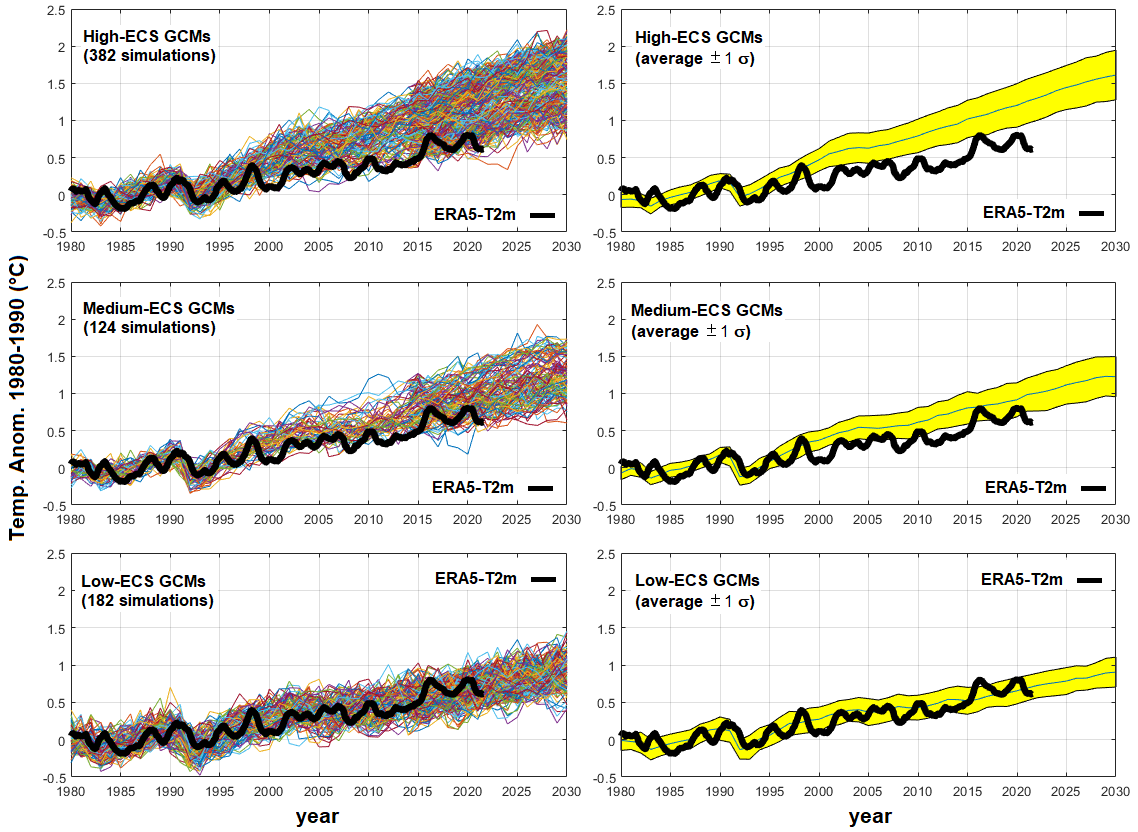
Figure 1: (Left) GCM global surface temperature simulations (colored curves) and (right) $\pm 1\sigma$ GCM global surface temperature ensembles (yellow area) versus the ERA5-T2m record (black, 12-month moving average).

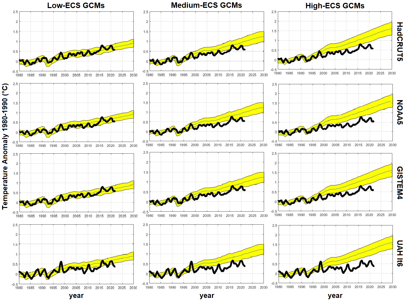
Figure 2: GCM global surface temperature ensembles (yellow area, $\pm 1\sigma$) versus HadCRUT5, GISTEMP v4, NOAAGlobTemp v5, and UAH-MSU-lt v6 temperature records (black, 12-month moving average).

2 Data and methods

We analyze the monthly reanalysis field near-surface air temperature (ERA5-T2m) record from 1980 to 2021 (Hersbach et al., 2020; Simmons et al., 2021). We repeat the same analysis using the HadCRUT5 (Morice et al., 2021), GISTEMP v4 (Lenssen et al., 2019), and NOAAGlobalTemp v5 (Zhang et al., 2019) global surface temperature records. Some of these records, however, may not cover the entire surface of the globe from 1980 to 2021. There are other global surface temperature records such as those proposed by the Japanese Meteorological Agency (JMA, Ishihara, 2006) and by the Berkeley Earth group (BE, Rohde and Hausfather, 2020), which will also be discussed briefly. For completeness, as explained in the Introduction, we add a comparison with the UAH-MSU-lt v6 temperature measurements (Spencer et al., 2017).

We also analyze all 143 “average” surface air temperature (tas) records and all 688 ensemble member records from 38 different CMIP6 GCMs downloadable from KNMI Climate Explorer. These simulations were produced using historical forcings (1850-2014) further extended up to 2100 with four different SSP scenarios: SSP1-2.6 (low GHG emissions), SSP2-4.5 (intermediate GHG emissions), SSP3-7.0 (high GHG emissions ) and SSP5-8.5 (very high greenhouse gas emissions) (IPCC, 2021). These four scenarios are nearly indistinguishable until 2021. Thus, from 1850 to 2021 the four simulation sets can be considered independent assessments of the same models under nearly identical forcing conditions, which also helps to assess in first approximation the internal variability of the models.

The 1980-2021 period was chosen to better evaluate the performance of the CMIP6 GCMs. This period is optimally covered by numerous climatic temperature records including those based on satellite measurements that are alternative to those based on land and oceanic measurements that could be affected by various non-climatic biases, which are difficult to eliminate (D’Aleo, 2016; Watts, 2022). In fact, going back in time from 1980 to 1850, the temperature records are affected by ever-larger uncertainties and uncovered areas, which makes evaluating the CMIP6 models even more difficult. A possible advantage of the present study is that the previous studies evaluating the performance of the CMIP6 models attempted to constrain the ECS by comparing GCM simulations only with surface climate records from 1850 to 2020 (Ribes et al., 2021) or from 1981 to 2014 (Tokarska et al., 2020), or even using uncertain paleoclimate records (Zhu et al., 2020) and concluded that only high-ECS models ($ECS>4.5$ ^∘C) could be excluded. However, there are open questions as to whether cooling adjustments applied to different Earth surface temperature records from 1850 to 1980 are justified (D’Aleo, 2016) and whether in more recent periods the global surface climate records are affected by non-climatic warming biases (Connolly et al., 2021; Scafetta, 2021a). These biases could have exaggerated the 20^th century warming trend and incorrectly provided support for the medium-ECS GCMs.

The 1980-2021 warming for each record is calculated by evaluating the 2011-2021 average temperature anomaly relative to the 1980-1990 period. 11-year intervals are used to bypass biases due to interannual fluctuations such as those related to ENSO and the 11-year solar cycle. Then, we apply standard statistical tests to decide if and how the observed warming values for each of the temperature records are reproduced by the three ECS GCM groups.

The ERA5-T2m global surface temperature average warming from 1980-1990 to 2011-2021 is estimated to be:

$$\Delta T_{mean}=0.578{{}^{\circ}}C.$$ (1)

The other temperature records give: HadCRUT5 (infilled data), $\Delta T_{mean}=0.581$^∘C; GISTEMP v4, $\Delta T_{mean}=0.570$^∘C; NOAAGlobalTemp v5, $\Delta T_{mean}=0.523$^∘C. HadCRUT5, GISTEMP, and ERA5-T2m give nearly identical warmings. We also observe that HadCRUT5 (non-infilled data) gives $\Delta T_{mean}=0.549$^∘C and HadCRUT4 gives $\Delta T_{mean}=0.521$^∘C. BE gives $\Delta T_{mean}=0.591$^∘C and JMA gives $\Delta T_{mean}=0.557$^∘C, which do not differ much from the above estimates. Thus, from 1980 to 2021, the available surface-based global temperature records measure that the global surface warming from 1980-1990 to 2011-2021 has been between 0.52^∘C and 0.59^∘C, or approximately between 0.50^∘C and 0.60^∘C, with an average of 0.56^∘C. In contrast, the satellite-based UAH-MSU-lt v6 temperature record gives $\Delta T_{mean}=0.402$^∘C, suggesting that 2011-2021 actual warming may have been even less than 0.40^∘C because, as explained in the introduction, according to the GCMs the temperature trend of the troposphere should be scaled down to make it compatible with the surface warming trend.

For the temperature records, since 1980 the error of the average over an 11-year period can be estimated to be very small, $\bar{\sigma}_{95\%}\approx 0.01$^∘C (see Appendix A), which represents about 2% of the warming from 1980-1990 to 2011-2021, and is less than the differences between the various temperature records.

As explained in the Introduction, the proposed analysis groups the CMIP6 GCMs into three subsets characterized by low ($1.5<ECS\leq 3.0$^∘C), medium ($3.0<ECS\leq 4.5$ ^∘C) and high ($4.5<ECS\leq 6.0$ ^∘C) sensitivity values. This choice is based on the following heuristic considerations. In fact, the IPCC (2013) estimated that the ECS had to have a “likely” range of 1.5 – 4.5^∘C. Also Wigley et al. (1997) suggested the same interval although the best-fit sensitivity was found to be 2.5°C. This range can be heuristically divided into at least two equal parts: $1.5<ECS\leq 3.0$ ^∘C and $3.0<ECS\leq 4.5$ ^∘C. In 2013, the CMIP5 GCMs were used. However, the IPCC (2021) adopted the CMIP6 GCMs that extended the ECS range up to 6^∘C so that an equally large third range, $4.5<ECS\leq 6.0$ ^∘C, could be added to the previous two. Zelinka et al. (2020) explained that the causes of the increased climate sensitivity in the CMIP6 models were due to stronger positive cloud feedbacks due to decreased extratropical cloud cover and albedo that, however, might be questionable.

Therefore, the interval $1.5<ECS\leq 3.0$ ^∘C collects the GCMs with ECS values most consistent with different empirical results, as discussed in the Introduction; the interval $3.0<ECS\leq 4.5$ ^∘C collects the other GCMs that also the IPCC (2013) would have considered acceptable; finally, the interval $4.5<ECS\leq 6.0$ ^∘C collects the GCMs included in the IPCC (2021) but which in 2013 the IPCC itself considered to predict an unlikely high ECS.

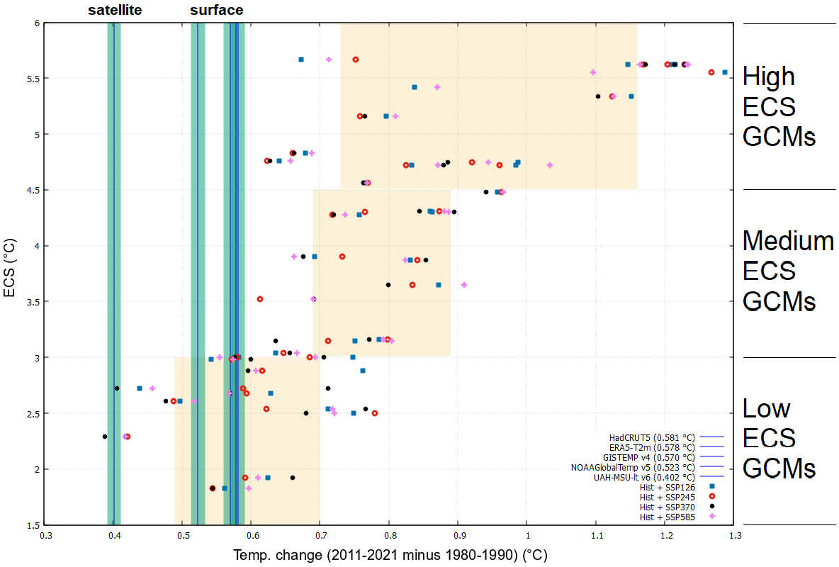
Figure 3: Average temperature changes (2011-2021 minus 1980-1990) hindcasted by 38 CMIP6 GCMs mean simulations. The blue vertical lines represent the temperature change measured by HadCRUT5, ERA5-T2m, GISTEMP v4, NOAAGlobTemp v5, and UAH-MSU-lt v6 temperature records, respectively, with their 95% confidence interval. The three yellow boxes represent the $\pm 1\sigma$ dispersion of the data referring to the low ($1.5<ECS\leq 3.0$ ^∘C), medium ($3.0<ECS\leq 4.5$ ^∘C) and high ($4.5<ECS\leq 6.0$ ^∘C) ECS GCMs. See Table 1.

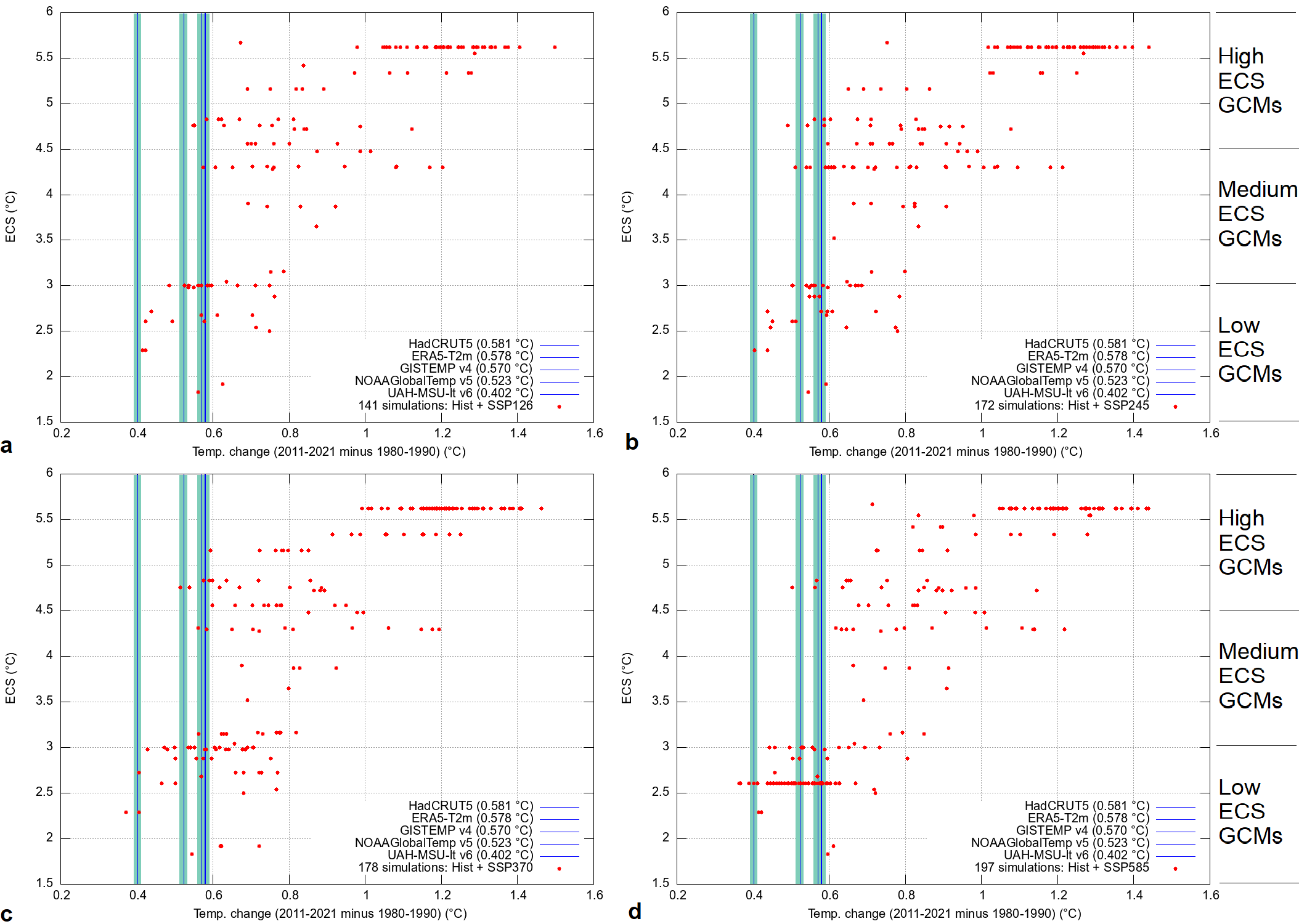
Figure 4: Temperature change (2011-2021 minus 1980-1990) hindcasted by the full range of model simulations (red dots). The vertical lines represents the global surface warming from 1980-1990 to 2011-2021 reported by HadCRUT5, ERA5-T2m, GISTEMP v4, NOAAGlobTemp v5, and UAH-MSU-lt v6 temperature records, respectively, with their 95% confidence interval. Each of the four panel represents a set of forcing: (a) Hist+SSP1-2.6, (b) Hist+SSP2-4.5, (c) Hist+SSP3-7.0 and (d) Hist+SSP5-8.5.

ECS GROUP	GCM	ECS (∘C)	SSP1-2.6 (∘C)	SSP2-4.5 (∘C)	SSP3-7.0 (∘C)	SSP5-8.5 (∘C)	$mean\pm 1\sigma$ (∘C)
High ECS	CIESM	5.67	0.67	0.75		0.71	$0.71\pm 0.04$
	CanESM5-CanOE-p2	5.62	1.15	1.17	1.17	1.16	$1.16\pm 0.01$
	CanESM5-p1	5.62	1.21	1.20	1.21	1.23	$1.22\pm 0.01$
	CanESM5-p2	5.62	1.22	1.23	1.23	1.23	$1.23\pm 0.01$
	HadGEM3-GC31-LL-f3	5.55	1.29	1.27		1.10	$1.22\pm 0.11$
	HadGEM3-GC31-MM-f3	5.42	0.84			0.87	$0.85\pm 0.02$
	UKESM1-0-LL-f2	5.34	1.15	1.12	1.10	1.13	$1.13\pm 0.02$
	CESM2	5.16	0.80	0.76	0.77	0.81	$0.78\pm 0.02$
	CNRM-CM6-1-f2	4.83	0.68	0.66	0.66	0.69	$0.67\pm 0.01$
	CNRM-ESM2-1-f2	4.76	0.64	0.62	0.63	0.66	$0.64\pm 0.02$
	CESM2-WACCM	4.75	0.99	0.92	0.89	0.94	$0.93\pm 0.04$
	ACCESS-CM2	4.72	0.83	0.82	0.88	0.87	$0.85\pm 0.03$
	NESM3	4.72	0.98	0.96		1.03	$0.99\pm 0.04$
	IPSL-CM6A-LR	4.56	0.76	0.77	0.76	0.77	$0.77\pm 0.01$
	$mean\pm 1\sigma$		$0.94\pm 0.23$	$0.94\pm 0.23$	$0.93\pm 0.23$	$0.94\pm 0.20$	$0.94\pm 0.23$
Medium ECS	KACE-1-0-G	4.48	0.96	0.96	0.94	0.97	$0.96\pm 0.01$
	EC-Earth3-Veg	4.31	0.86	0.87	0.84	0.88	$0.86\pm 0.02$
	EC-Earth3	4.3	0.86	0.76	0.90	0.89	$0.85\pm 0.06$
	CNRM-CM6-1-HR-f2	4.28	0.76	0.72	0.72	0.74	$0.73\pm 0.02$
	GFDL-ESM4	3.9	0.69	0.73	0.68	0.66	$0.69\pm 0.03$
	ACCESS-ESM1-5	3.87	0.83	0.84	0.85	0.82	$0.84\pm 0.01$
	MCM-UA-1-0	3.65	0.87	0.83	0.80	0.91	$0.85\pm 0.05$
	CMCC-CM2-SR5	3.52		0.61	0.69	0.69	$0.66\pm 0.04$
	AWI-CM-1-1-MR	3.16	0.79	0.80	0.77	0.79	$0.79\pm 0.01$
	MRI-ESM2-0	3.15	0.75	0.71	0.64	0.80	$0.73\pm 0.07$
	BCC-CSM2-MR	3.04	0.64	0.65	0.66	0.67	$0.65\pm 0.01$
	$mean\pm 1\sigma$		$0.80\pm 0.10$	$0.77\pm 0.10$	$0.77\pm 0.10$	$0.80\pm 0.10$	$0.79\pm 0.10$
Low ECS	FGOALS-f3-L	3	0.75	0.69	0.71	0.69	$0.71\pm 0.03$
	MPI-ESM1-2-LR	3	0.58	0.58	0.58	0.56	$0.57\pm 0.01$
	MPI-ESM1-2-HR	2.98	0.54	0.57	0.60	0.57	$0.57\pm 0.02$
	FGOALS-g3	2.88	0.76	0.62	0.60	0.61	$0.65\pm 0.08$
	GISS-E2-1-G-p1	2.72			0.71		$0.71$
	GISS-E2-1-G-p3	2.72	0.44	0.59	0.41	0.46	$0.47\pm 0.08$
	MIROC-ES2L-f2	2.68	0.63	0.59	0.57	0.57	$0.59\pm 0.03$
	MIROC6	2.61	0.50	0.49	0.48	0.52	$0.50\pm 0.02$
	NorESM2-LM	2.54	0.71	0.62	0.77	0.72	$0.70\pm 0.06$
	NorESM2-MM	2.5	0.75	0.78	0.68	0.72	$0.73\pm 0.04$
	CAMS-CSM1-0	2.29	0.42	0.42	0.39	0.42	$0.41\pm 0.02$
	INM-CM5-0	1.92	0.62	0.59	0.66	0.61	$0.62\pm 0.03$
	INM-CM4-8	1.83	0.56	0.54	0.54	0.60	$0.56\pm 0.02$
	$mean\pm 1\sigma$		$0.61\pm 0.12$	$0.59\pm 0.09$	$0.59\pm 0.12$	$0.59\pm 0.09$	$0.60\pm 0.12$

Table 1: Warming from 1980-1990 to 2011-2021 for average simulations of 38 GCMs using Historical + SSP1-2.6, SSP2-4.5, SSP3-7.0, and SSP5-8.5 forcings. See Figure 3.

ECS GROUP		SSP1-2.6	SSP2-4.5	SSP3-7.0	SSP5-8.5	total	%
	total members	141	172	178	197	688
High ECS	$\mathrm{Model>HadCRUT}$	86	93	97	93	369	97%
	$\mathrm{Model>ERA5T2m}$	86	93	97	93	369	97%
	$\mathrm{Model>GISTEMP}$	88	93	98	93	372	98%
	$\mathrm{Model>NOAAGT}$	88	95	100	96	379	99.5%
	$\mathrm{Model>UAHMSU}$	88	96	100	96	380	100%
	$\mathrm{Model<HadCRUT}$	2	3	3	3	11	3%
	$\mathrm{Model<ERA5T2m}$	2	3	3	3	11	3%
	$\mathrm{Model<GISTEMP}$	0	3	2	3	8	2%
	$\mathrm{Model<NOAAGT}$	0	1	0	0	1	0.5%
	$\mathrm{Model<UAHMSU}$	0	0	0	0	0	0%
Medium ECS	$\mathrm{Model>HadCRUT}$	25	39	29	26	119	94%
	$\mathrm{Model>ERA5T2m}$	25	39	30	26	120	95%
	$\mathrm{Model>GISTEMP}$	26	39	30	26	121	96%
	$\mathrm{Model>NOAAGT}$	26	41	32	26	125	99%
	$\mathrm{Model>UAHMSU}$	26	42	32	26	126	100%
	$\mathrm{Model<HadCRUT}$	1	3	3	0	7	6%
	$\mathrm{Model<ERA5T2m}$	1	3	2	0	6	5%
	$\mathrm{Model<GISTEMP}$	0	3	2	0	5	4%
	$\mathrm{Model<NOAAGT}$	0	1	0	0	1	1%
	$\mathrm{Model<UAHMSU}$	0	0	0	0	0	0%
Low ECS	$\mathrm{Model>HadCRUT}$	12	14	25	18	69	38%
	$\mathrm{Model>ERA5T2m}$	12	15	26	19	72	40%
	$\mathrm{Model>GISTEMP}$	13	16	28	24	81	45%
	$\mathrm{Model>NOAAGT}$	21	26	35	39	121	66%
	$\mathrm{Model>UAHMSU}$	27	33	43	71	174	96%
	$\mathrm{Model<HadCRUT}$	15	20	21	57	113	62%
	$\mathrm{Model<ERA5T2m}$	15	19	20	56	110	60%
	$\mathrm{Model<GISTEMP}$	14	18	18	51	101	55%
	$\mathrm{Model<NOAAGT}$	6	8	11	36	61	34%
	$\mathrm{Model<UAHMSU}$	0	1	3	4	8	4%

Table 2: Number of single GCM simulations reporting mean temperature changes (2011-2021 minus 1980-1990) lower or higher than HadCRUT5, ERA5-T2m, GISTEMP v4, NOAAGlobTemp v5 and UAH-MSU-lt v6, respectively.

3 Analysis of the CMIP6 GCM simulations

Figure 1 shows the GCM simulations (left) and their ensemble $mean\pm 1\sigma$ range (right) grouped according to the three GCM ECS sets with respect to the ERA5-T2m global surface temperature record (black, moving averages at 12 months). All records are temperature anomalies relative to the period 1980-1990. Figure 2 shows a similar comparison with respect to the HadCRUT, GISTEMP, NOAAGlobTemp and UAH-MSU-lt temperature records.

Both figures show that as the ECS increases, the global surface warming predicted by the models also increases. However, only the low-ECS GCM group can be considered perfectly consistent with the surface-based global temperature records because it encloses them well within the $\pm 1$$\sigma$ GCM range (yellow area).

Figures 1 and 2 also show that, compared to the satellite record, even the GCM group with low ECS seems to overestimate the observed warming. In fact, even for the low ECS GCM group from 2011 to 2021 the UAH-MSU-lt record is not well enclosed within the $\pm 1\sigma$ model ensemble (yellow) area although a better agreement is found in the period 2015- 2020. The latter was characterized by the significant El Niño warming events of 2015-2016 and 2020 (Appendix A, Figure 11). Therefore, the 2015-2020 warming for the period 2000-2014 could also be temporary (Scafetta, 2021c) and not related to the warming hindcasted by the models because it is clearly due to natural climatic fluctuations while the average warming produced by the models is due to anthropogenic forcing. From 2015 to 2022, in fact, a slightly cooling trend is observed. From 2000 to 2014 the UAH-MSU-lt v6 record also clearly shows the so-called global warming “hiatus” or “pause” (IPCC, 2013). This decade-long lack of warming began to seriously question the GCMs, and various statistical solutions were proposed to circumvent the problem by referring to the fluctuations of the internal variability of the climate system (e.g. Meehl et al., 2011). Figures 1 and 2 also show that, at the present, the "pause" appears missing or attenuated in the latest versions of the surface-based  global temperature records.

3.1 Analysis of the GCM average simulations

Scafetta (2022) analyzed the average simulations of 38 GCMs using the historical + SSP2-4.5, SSP3-7.0, and SSP5-8.5 radiative forcing scenarios up to June 2021; the warming values for each model were collected in the table there published. Figure 3 graphically shows the results of the same analysis, which was updated to the whole year 2021 and also included the SSP1-2.6 simulations, compared to the temperature observations (green vertical lines). 143 average records are analyzed. For each ECS GCM group the statistics provide (see Table 1):

• High-ECS GCMs (51 records): $\Delta T_{mean}=0.94\pm 0.22$ ^∘C;

• Medium-ECS GCMs (43 records): $\Delta T_{mean}=0.79\pm 0.10$ ^∘C;

• Low-ECS GCMs (49 records): $\Delta T_{mean}=0.59\pm 0.10$ ^∘C.

The result confirms that the GCM group with low ECS is perfectly compatible with the observed warming (Eq. 1) within the $\pm 1$$\sigma$ range. In contrast, both GCM groups with medium and high ECS show warming biases. Moreover, as Scafetta (2022) already observed, Figure 3 also shows that none of the medium and high ECS models predict an average warming of less than 0.6^∘C, which is above the warming reported by all global temperature surface records. This result suggests that models with $ECS>3$^∘C should be questioned at the 95% confidence level. Thus, by considering only the GCM ensemble averages for the four SSPs, the real ECS should be equal to or lower than 3^∘C.

However, Figure 3 also shows that if the UAH-MSU-LT record better reproduces the actual 2011-2021 warming, the GCM group with low ECS would also be too hot because, out of 49 GCM ensemble averages with low ECS, 48 cases (98%) are warmer than 0.40^∘C. The GCM that best agrees with the satellite record is CAMS-CSM1-0 whose ECS is 2.29^∘C.

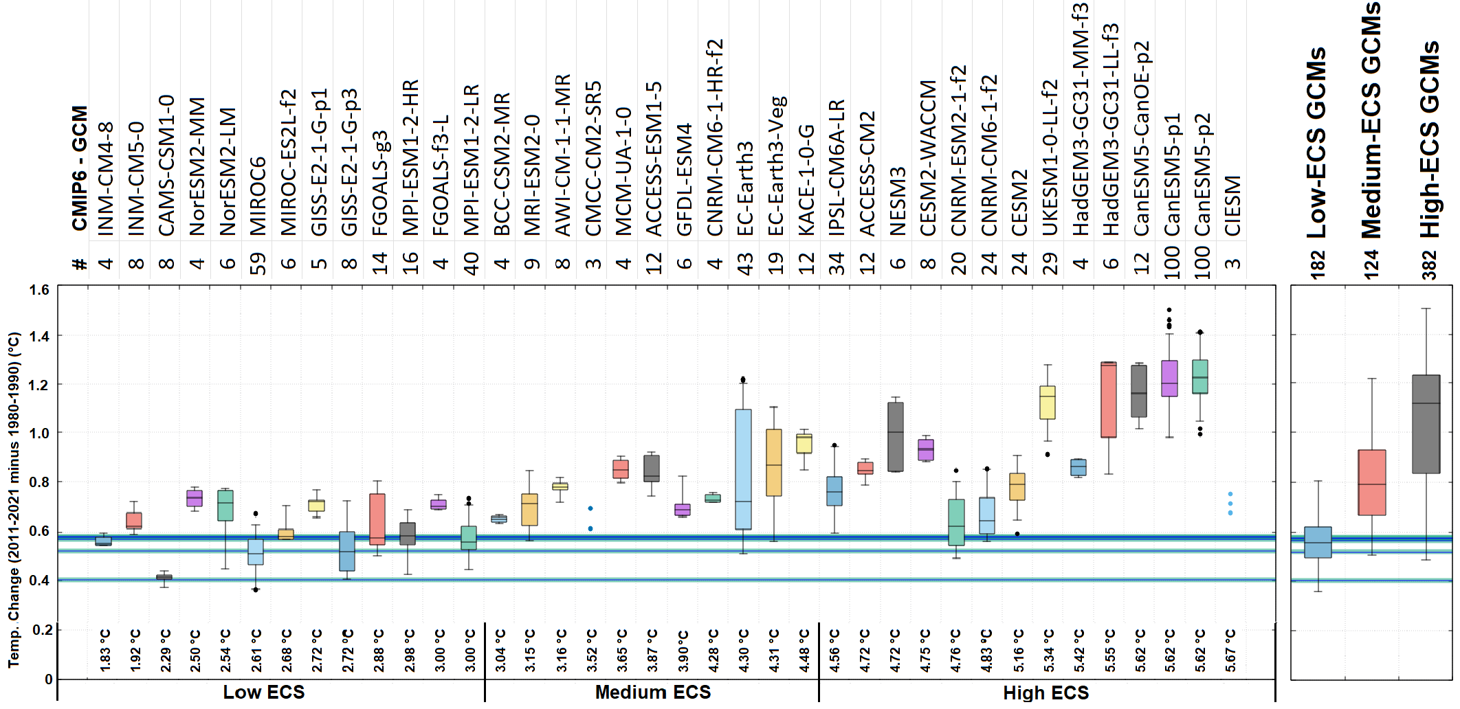
Figure 5: Boxplots of the CMIP6 ensemble members depicted in Figure 4 for each CMIP6 GCM; # represents the number of the available simulations for each GCM. The horizontal blue lines represents the global surface warming from 1980-1990 to 2011-2021 reported by HadCRUT5, ERA5-T2m, GISTEMP v4, NOAAGlobTemp v5, and UAH-MSU-lt v6 temperature records, respectively. The whiskers extend from each end of the box for a range up to 1.5 times the interquartile range.

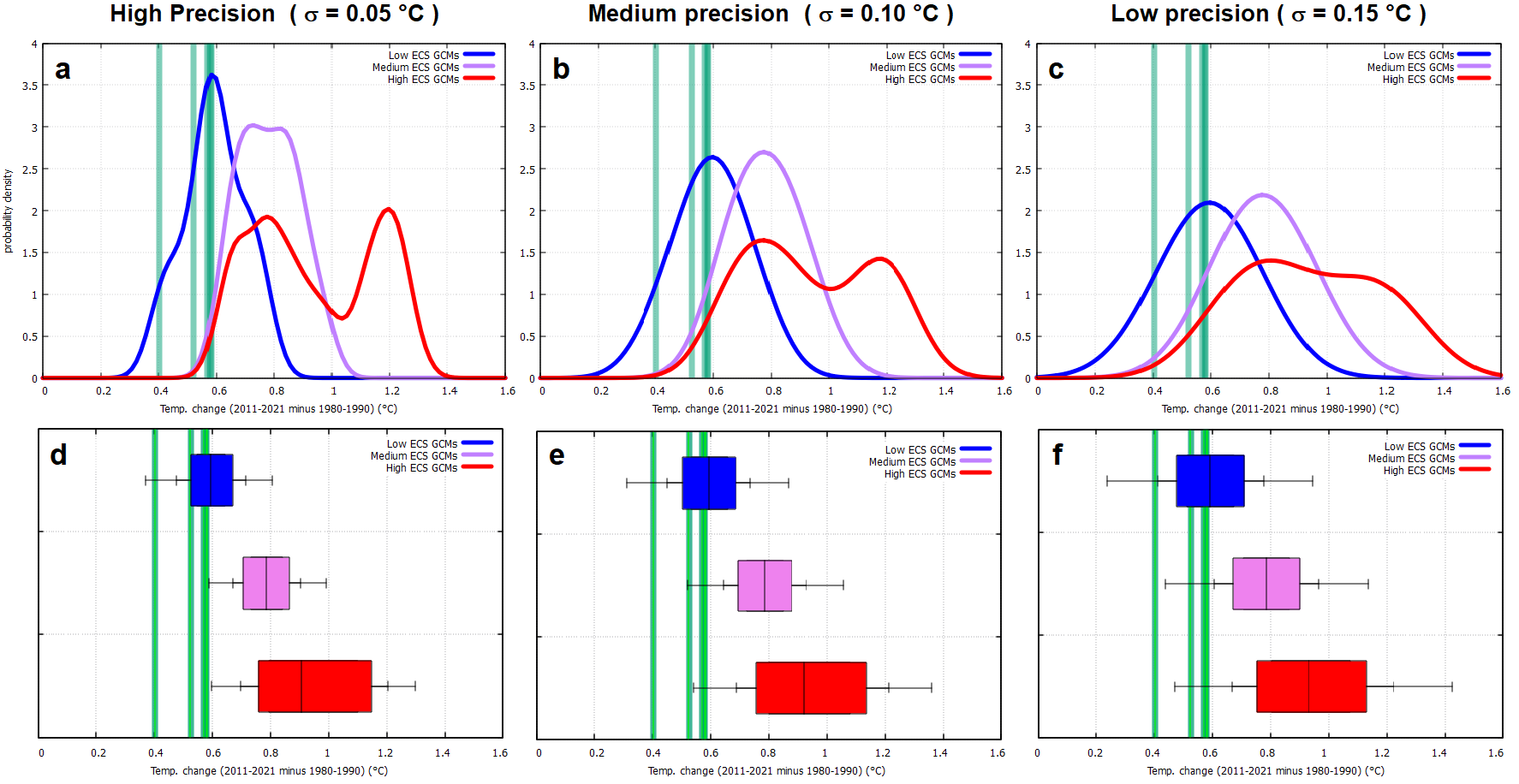
Figure 6: (a, b, c) GCM probability density functions relative to three model precision requirements: $\sigma=0.05$^∘C, $\sigma=0.10$^∘C and $\sigma=0.15$^∘C, which approximately correspond to $\sigma_{95\%}=0.10$^∘C, $\sigma_{95\%}=0.20$^∘C and $\sigma_{95\%}=0.30$^∘C. The green vertical lines represent the global surface warming from 1980-1990 to 2011-2021 reported by HadCRUT5, ERA5-T2m, GISTEMP v4, NOAAGlobTemp v5 and UAH-MSU-lt v6 temperature records. (d, e, f) Boxplots of the the probability density functions depicted in panels a, b, c, respectively, using double whiskers and boxes indicating the following probability ranges: 2.5%, 16%, 25%, 50%, 75%, 84% and 97.5%.

3.2 Analysis of the full range of the GCM ensemble members

Figure 4 shows in four panels the temperature variations (2011-2021 minus 1980-1990) of the 688 simulations of GCM ensemble members available per forcing set (Hist+SSP1-2.6, Hist+SSP2-4.5, Hist+SSP3-7.0 and Hist+SSP5-8.5; red dots) against the five temperature records (vertical lines). The figure visually confirms that the vast majority of ensemble member simulations produced by the GCM groups with medium and high ECS run too hot relative to all five temperature records.

To examine how observed warming values are placed within the distributions of possible GCM hindcasts for each of the three ECS groups, we count how many member simulations record temperatures colder or warmer than each of the five temperature records. Table 2 reports the results.

The analysis confirms that the low-ECS models produce results that well enclose the 2011-2021 average temperatures obtained using the surface temperature temperature records, which always fall within the statistical interval $\pm 1\sigma$ (corresponding to the 16-84% probability interval) of the distribution of the GCM hindcasts. In contrast, 94-100% and 97-100% of hindcasts produced by the GCMs with medium and high ECS are warmer than all five temperature records, respectively. Therefore, also considering the full range of the available CMIP6 GCM simulations, the GCMs with medium and high ECS run too hot. Thus, the actual ECS should be equal to or less than 3^∘C.

However, 96% of GCM simulations from the low-ECS GCM are warmer and only 4% cooler than the lower troposphere temperature record. So, once again, we found that if UAH-MSU-lt better reproduces the actual global warming from 1980-1990 to 2011-2021, the vast majority of the low-ECS GCM ensemble members would also be found to run too hot.

ECS GROUP		high precision	medium precision	low precision
		( $\sigma_{H}=0.05$∘C)	( $\sigma_{M}=0.10$∘C)	( $\sigma_{L}=0.15$∘C)
High ECS	$\mathrm{HadCRUT<Model}$	99%	95%	92%
	$\mathrm{ERA5T2m<Model}$	99%	95%	92%
	$\mathrm{GISTEMP<Model}$	99%	96%	93%
	$\mathrm{NOAAGT<Model}$	100%	98%	95%
	$\mathrm{UAHMSU<Model}$	100%	100%	99%
	$\mathrm{HadCRUT>Model}$	1%	5%	8%
	$\mathrm{ERA5T2m>Model}$	1%	5%	8%
	$\mathrm{GISTEMP>Model}$	1%	4%	7%
	$\mathrm{NOAAGT>Model}$	0%	2%	5%
	$\mathrm{UAHMSU>Model}$	0%	0%	1%
Medium ECS	$\mathrm{HadCRUT<Model}$	98%	93%	88%
	$\mathrm{ERA5T2m<Model}$	98%	93%	88%
	$\mathrm{GISTEMP<Model}$	99%	94%	88%
	$\mathrm{NOAAGT<Model}$	100%	97%	93%
	$\mathrm{UAHMSU<Model}$	100%	100%	99%
	$\mathrm{HadCRUT>Model}$	2%	7%	12%
	$\mathrm{ERA5T2m>Model}$	2%	7%	12%
	$\mathrm{GISTEMP>Model}$	1%	6%	12%
	$\mathrm{NOAAGT>Model}$	0%	3%	7%
	$\mathrm{UAHMSU>Model}$	0%	0%	1%
Low ECS	$\mathrm{HadCRUT<Model}$	55%	54%	53%
	$\mathrm{ERA5T2m<Model}$	56%	55%	53%
	$\mathrm{GISTEMP<Model}$	59%	57%	55%
	$\mathrm{NOAAGT<Model}$	74%	69%	65%
	$\mathrm{UAHMSU<Model}$	95%	91%	85%
	$\mathrm{HadCRUT>Model}$	45%	46%	47%
	$\mathrm{ERA5T2m>Model}$	44%	45%	47%
	$\mathrm{GISTEMP>Model}$	41%	43%	45%
	$\mathrm{NOAAGT>Model}$	26%	31%	35%
	$\mathrm{UAHMSU>Model}$	5%	9%	15%

Table 3: Probability $P_{\Delta T<GCMs}$ and $P_{\Delta T>GCMs}$ that the 2011-2021 warming hindcast from 1980-1990 to 2011-2021 for each ECS GCM ensemble is warmer or colder, respectively, than HadCRUT5, ERA5- T2m, GISTEMP v4, NOAAGlobTemp v5 and UAH-MSU-lt v6, respectively: see Figure 6.

	Observations and GCM hindcasts				Modeled Global and Land Warmings
(80∘S:80∘N)	Total (∘C)	Land (∘C)	Ocean (∘C)	ratio	Total (∘C)	Land (∘C)	Ocean (∘C)	average ratio
HadCRUT5	0.57	0.86	0.45	1.92	0.54	0.76	0.45	1.69
ERA5-T2m	0.57	0.92	0.43	2.14	0.51	0.73	0.43	1.69
GISTEMP	0.54	0.93	0.41	2.26	0.48	0.69	0.41	1.69
NOAAGT	0.53	0.91	0.38	2.38	0.45	0.64	0.38	1.69
MSU-UAH	0.40	0.53	0.34	1.54	0.41	0.57	0.34	1.69
Low ECS GCMs	0.58$\pm$0.10	0.84$\pm$0.18	0.48$\pm$0.08	1.73$\pm$0.21
Medium ECS GCMs	0.77$\pm$0.10	1.07$\pm$0.15	0.66$\pm$0.08	1.63$\pm$0.13
High ECS GCMs	0.92$\pm$0.21	1.31$\pm$0.28	0.78$\pm$0.19	1.71$\pm$0.22
(60∘S:80∘N)	Total (∘C)	Land (∘C)	Ocean (∘C)	ratio	Total (∘C)	Land (∘C)	Ocean (∘C)	average ratio
HadCRUT5	0.59	0.91	0.47	1.95	0.56	0.82	0.47	1.74
ERA5-T2m	0.61	0.97	0.47	2.08	0.57	0.82	0.47	1.74
GISTEMP	0.55	0.94	0.42	2.24	0.50	0.73	0.42	1.74
NOAAGT	0.54	0.91	0.39	2.32	0.47	0.68	0.39	1.74
MSU-UAH	0.42	0.55	0.37	1.51	0.42	0.54	0.37	1.74
Low ECS GCMs	0.59$\pm$0.11	0.86$\pm$0.19	0.49$\pm$0.08	1.75$\pm$0.20
Medium ECS GCMs	0.77$\pm$0.11	1.10$\pm$0.16	0.65$\pm$0.09	1.69$\pm$0.14
High ECS GCMs	0.92$\pm$0.21	1.34$\pm$0.29	0.76$\pm$0.19	1.79$\pm$0.24
(0∘N:80∘N)	Total (∘C)	Land (∘C)	Ocean (∘C)	ratio	Total (∘C)	Land (∘C)	Ocean (∘C)	average ratio
HadCRUT5	0.81	1.03	0.68	1.52	0.79	0.99	0.68	1.45
ERA5-T2m	0.85	1.09	0.69	1.57	0.82	1.00	0.69	1.45
GISTEMP	0.78	1.04	0.63	1.66	0.73	0.91	0.63	1.45
NOAAGT	0.75	1.00	0.59	1.72	0.69	0.86	0.59	1.45
MSU-UAH	0.48	0.56	0.42	1.32	0.50	0.61	0.42	1.45
Low ECS GCMs	0.77$\pm$0.18	0.95$\pm$0.23	0.66$\pm$0.16	1.45$\pm$0.12
Medium ECS GCMs	1.00$\pm$0.17	1.21$\pm$0.19	0.87$\pm$0.16	1.40$\pm$0.09
High ECS GCMs	1.20$\pm$0.32	1.47$\pm$0.35	1.02$\pm$0.31	1.49$\pm$0.28
(60∘S:0∘S)	Total (∘C)	Land (∘C)	Ocean (∘C)	ratio	Total (∘C)	Land (∘C)	Ocean (∘C)	average ratio
HadCRUT5	0.34	0.58	0.29	1.97	0.33	0.50	0.29	1.72
ERA5-T2m	0.34	0.64	0.29	2.25	0.32	0.50	0.29	1.72
GISTEMP	0.30	0.61	0.26	2.40	0.28	0.45	0.26	1.72
NOAAGT	0.31	0.65	0.24	2.68	0.27	0.41	0.24	1.72
MSU-UAH	0.35	0.54	0.32	1.67	0.34	0.46	0.32	1.72
Low ECS GCMs	0.39$\pm$0.08	0.60$\pm$0.13	0.35$\pm$0.08	1.75$\pm$0.41
Medium ECS GCMs	0.51$\pm$0.08	0.76$\pm$0.12	0.47$\pm$0.08	1.64$\pm$0.29
High ECS GCMs	0.61$\pm$0.13	0.96$\pm$0.33	0.55$\pm$0.11	1.77$\pm$0.54

Table 4: Left columns: observed and hindcasted warming over 80^∘S:80^∘N, 60^∘S:80^∘N, 0^∘N:80^∘N, and 60^∘S:0^∘S latitude ranges from 1980-1990 to 2011-2021 over land+ocean (total), land, and ocean, and land/ocean ratio. The model estimates use the average GCM simulations. Right columns: global and land warming calculated assuming correct the ocean warming reported by the temperature records and the average land/ocean warming ratios hindcasted by the GCMs.

3.3 Statistical modeling of the GCM unforced internal variability

Figure 5 shows the boxplots relating to the simulations shown in Figure 4 for each model. Again, the GCM group with low ECS is best centered around the surface-based observations indicated by the horizontal blue lines while the GCM groups with medium and high ECS exhibit systematic warming bias except for very few models. However, the dispersion of the boxplots varies greatly among the GCMs because the models are not physically equivalent to each other and, furthermore, probably because of the different number of simulations available for each model.

In fact, the GCMs are represented unevenly in the KNMI collection because the number of simulations available for each GCM varies from 3 to 100 among the models: see Figure 5. Therefore, the statistics discussed in Section 3.2 may be skewed towards models with a larger number of available simulations because they will weight more in the statistical test reported in Table 3. This problem could be solved by using a Monte Carlo strategy to simulate the spread of GCM hindcasts that could be associated with unforced internal variability. This exercise is proposed below.

It can be assumed that each GCM produces simulations distributed around a mean $\mu_{m}$ with a given standard deviation $\sigma_{m}$ characterizing its internal variability. We note that $\sigma_{m}$ should be assumed constant for all GCM averages because it could be interpreted as a “precision” requirement for GCMs. Indeed, GCM hindcasts should always agree with observations within an acceptable statistical uncertainty.

We propose three different options for $\sigma_{m}$ covering approximately the ranges of the GCM boxplots shown in Figure 5: $\sigma_{H}\approx 0.05$^∘C (high precision), $\sigma_{M}\approx 0.10$^∘C (medium precision), and $\sigma_{L}\approx 0.15$^∘C (low precision).

Figure 5 suggests that the high-precision option ($\sigma_{H}\approx 0.05$^∘C) could be satisfied by most GCMs; it requires the model mean to be within $\pm 0.1$^∘C (95% confidence interval) of the actual warming value. The 95% confidence range becomes $\pm 0.2$^∘C for the medium-precision requirement ($\sigma_{M}\approx 0.10$^∘C) and $\pm 0.3$^∘C for the low-precision option ($\sigma_{L}\approx 0.15$^∘C).

Appendix B shows that the interval $\pm 0.1$^∘C (95% confidence), which corresponds to the high precision option, $\sigma_{H}\approx 0.05$^∘C, should be the preferred choice for the acceptable uncertainty related to the internal variability that should be requested for the GCM because it could be derived from the variability of the temperature records themselves.

Figure 5 also shows that the low-precision option $\sigma_{L}\approx 0.15$^∘C is only consistent with the EC-Earth3 GCM. The usefulness of this model should be questioned because it hindcasts 2011-2021 global surface warming values ranging between 0.5^∘C to 1.2^∘C with an average of 0.82^∘C. This means that EC-Earth3 is both inaccurate and imprecise in hindcasting the global surface warming from 1980 to 2021.

Figure 6 shows the combined probability density functions (PDF) and the related boxplots derived from all the GCM means reported in Figure 3 and in Table 1 with the three precision requirements for the three ECS GCM groups compared to the warming levels obtained with the adopted five temperature records. The complementary Gaussian error function was used to evaluate the relative statistical position of the five actual warming values within each probability density function.

For each model mean $\mu_{m}$ and precision $\sigma$, the probability $P_{m}$ that the GCM hindcast is larger than the measured warming $\Delta T$ is

$$P_{m}=\frac{1}{\sigma\sqrt{2\pi}}\intop_{\Delta T}^{\infty}e^{-\frac{(t-\mu_{m})}{2\sigma^{2}}^{2}}\,dt=\frac{1}{2}\,\mathrm{erfc}\left(\frac{\Delta T-\mu_{m}}{\sigma\sqrt{2}}\right).$$ (2)

Thus, the mean $P_{\Delta T<GCMs}=\frac{1}{N}\sum_{m=1}^{N}P_{m}$ across all models for each ECS GCM group gives the probability of obtaining simulations warmer than the reference temperature value. $P_{\Delta T<GCMs}$ can also be obtained by integrating the probability density functions shown in Figure 6a-6c from the green line to infinity or by using a Monte Carlo strategy by generating, for example, 1000 computer values from a Gaussian distribution with mean $\mu_{m}$ and standard deviation $\sigma$. The relevant statistics are shown in Table 3.

Figure 6a-6c show that the GCM group with low ECS (blue curves) always produces predictions well-centered on the observed warming for the four surface temperature records because their 2011-2021 values always fall within the $\pm 1\sigma$ statistical interval (which corresponds to the 16%-84% probability range) of the GCM distributions for the high, medium, and low precision options, respectively. However, once again, if the actual 1980-2021 warming is given by UAH-MSU-lt, even the GCM group with low ECS seems to be biased towards too hot values in 95%, 91% and 85% of possible cases, respectively, for the three precision options (Table 3).

The predictions of the medium (purple) and high (red) ECS GCM groups always show significant warming biases. Also, particularly for the GCM group with high ECS, the PDF appears to have two peaks, implying that the GCMs in this group are physically very different from each other because they produce very different warming hindcasts that are clustered around 0.8^∘C and 1.2^∘C; the warmest PDF peak is mostly due to the CanESM5 GCM.

For the high-precision requirement ($\sigma_{H}=0.05$^∘C), these two GCM groups produce results warmer than the observed values from a minimum of 98% to a maximum of 100% of their possible output, which is outside the 95% confidence interval. For the medium precision option ($\sigma_{M}=0.10$^∘C), the medium and high GCM groups produce results warmer than the observed values from a minimum of 93% to a maximum of 100% of their possible outputs, which is at the limit of the 95% confidence interval. For the low precision option ($\sigma_{L}=0.15$^∘C), the GCM groups with medium and high ECS produce warmer results than the four surface-based temperature records from 88% to 95% of cases. Conversely, 99% or more of the theoretical hindcasts of the GCM groups with high and medium ECS would be warmer than UAH-MSU-lt even for the low precision option ($\sigma_{L}=0.15$^∘C).

The boxplots illustrated in Figures 6d-6f were obtained using the Monte Carlo strategy proposed above which simulates 1000 randomly distributed outputs for each of the 143 model averages for each of the three precision options (for a total of $3\times 143,000$ theoretical hindcasts). The three panels show that in all cases, with respect to the observed temperature values, the groups with medium and high ECS are well outside the 68% confidence interval (i.e. the $\pm 1\sigma$ interval). Furthermore, the GCM groups with medium and high ECS indicate levels of warming that are respectively 30% and 50% greater than those actually observed and, consequently, their accuracy is rather low. The accuracy of the low-ECS GCM group is good compared to the surface-based temperature records, but it still reports average warming that is about 30% larger than that reported by the satellite temperature record. The whisker extension of the boxplot shows that the precision of the low, medium and high ECS groups varies from modest ($\pm 0.2$^∘C) to very poor ($\pm 0.5$^∘C) range from low ECS and high precision GCM group to high and low precision GCM group.

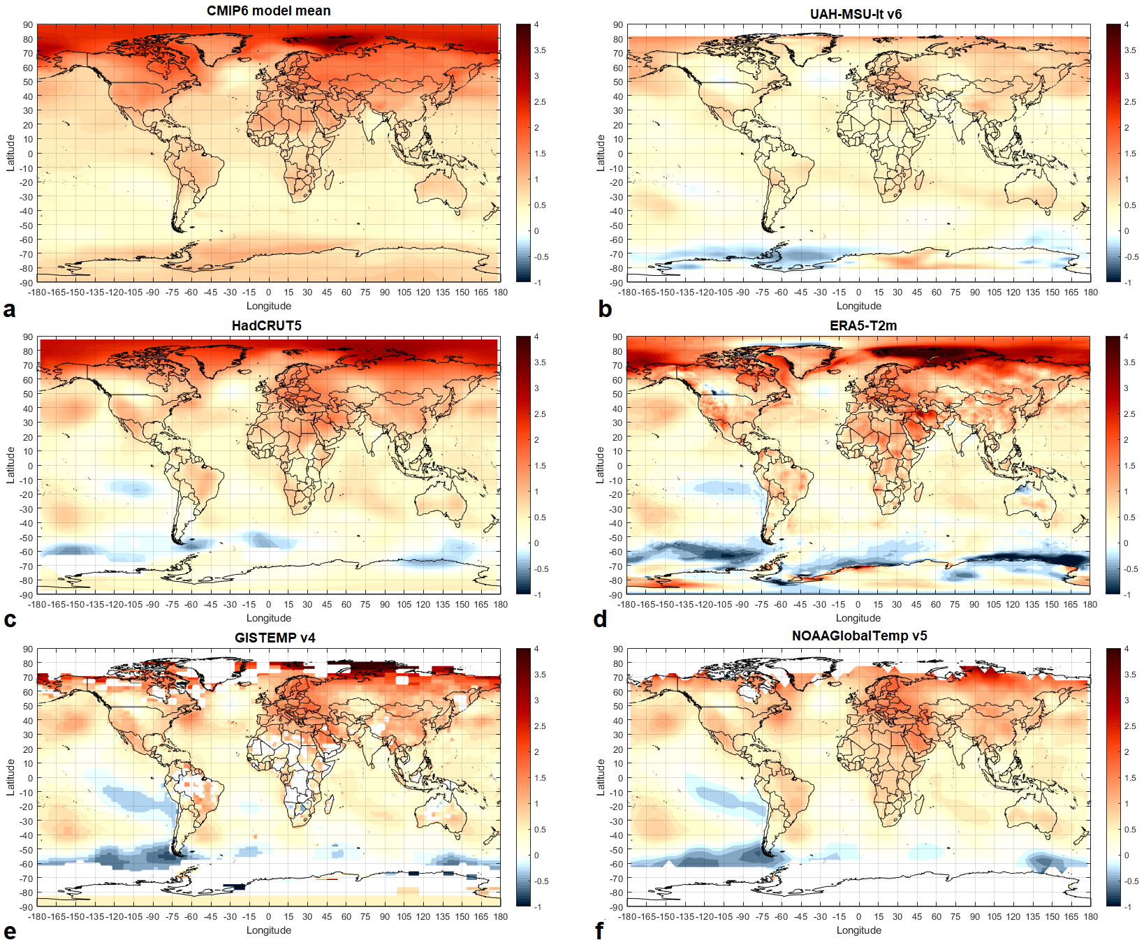
Figure 7: Areal distribution of the warming from 1980-1990 to 2011-2021 for the CMIP6 ensemble average simulation and for the HadCRUT5, ERA5-T2m, GISTEMP v4, NOAAGlobTemp v5, and UAH-MSU-lt v6 temperature records.

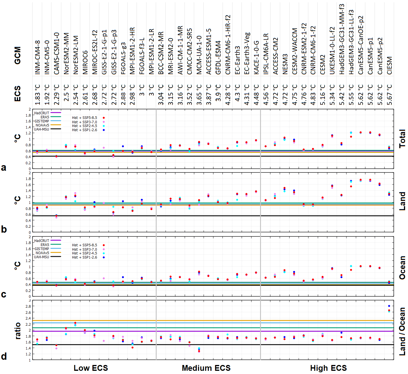
Figure 8: 2011-2021 warming relative to 1980-1990 of the models over (a) land+ocean, (b) land, (c) ocean areas within the 60^∘S:80^∘N latitude range for the 143 average model simulations (colored dots) and the five temperature records (colored lines). (d) Ratio between the land and the ocean warming. See Tables 5, 6, and 7.

Model	ECS (∘C)	Hist + SSP	Land + Ocean (∘C)	Land (∘C)	Ocean (∘C)	Land/Ocean
INM-CM4-8	1.83	SSP1-2.6	0.55	0.78	0.46	1.69
INM-CM4-8	1.83	SSP2-4.5	0.54	0.72	0.47	1.54
INM-CM4-8	1.83	SSP3-7.0	0.52	0.72	0.45	1.62
INM-CM4-8	1.83	SSP5-8.5	0.58	0.82	0.49	1.68
INM-CM5-0	1.92	SSP1-2.6	0.59	0.83	0.50	1.66
INM-CM5-0	1.92	SSP2-4.5	0.56	0.82	0.46	1.76
INM-CM5-0	1.92	SSP3-7.0	0.64	0.92	0.53	1.74
INM-CM5-0	1.92	SSP5-8.5	0.59	0.84	0.49	1.73
CAMS-CSM1-0	2.29	SSP1-2.6	0.43	0.57	0.38	1.50
CAMS-CSM1-0	2.29	SSP2-4.5	0.42	0.56	0.37	1.50
CAMS-CSM1-0	2.29	SSP3-7.0	0.39	0.49	0.35	1.39
CAMS-CSM1-0	2.29	SSP5-8.5	0.42	0.55	0.37	1.49
NorESM2-MM	2.5	SSP1-2.6	0.77	1.16	0.62	1.86
NorESM2-MM	2.5	SSP2-4.5	0.80	1.20	0.64	1.87
NorESM2-MM	2.5	SSP3-7.0	0.71	1.11	0.55	2.03
NorESM2-MM	2.5	SSP5-8.5	0.74	1.18	0.57	2.06
NorESM2-LM	2.54	SSP1-2.6	0.74	1.21	0.56	2.17
NorESM2-LM	2.54	SSP2-4.5	0.64	1.04	0.48	2.15
NorESM2-LM	2.54	SSP3-7.0	0.79	1.31	0.59	2.23
NorESM2-LM	2.54	SSP5-8.5	0.74	1.23	0.55	2.24
MIROC6	2.61	SSP1-2.6	0.51	0.78	0.41	1.91
MIROC6	2.61	SSP2-4.5	0.50	0.77	0.40	1.92
MIROC6	2.61	SSP3-7.0	0.49	0.75	0.39	1.92
MIROC6	2.61	SSP5-8.5	0.53	0.83	0.41	2.00
MIROC-ES2L-f2	2.68	SSP1-2.6	0.65	1.00	0.51	1.98
MIROC-ES2L-f2	2.68	SSP2-4.5	0.61	0.92	0.49	1.87
MIROC-ES2L-f2	2.68	SSP3-7.0	0.58	0.84	0.48	1.76
MIROC-ES2L-f2	2.68	SSP5-8.5	0.58	0.87	0.48	1.82
GISS-E2-1-G-p1	2.72	SSP3-7.0	0.70	0.98	0.60	1.63
GISS-E2-1-G-p3	2.72	SSP1-2.6	0.45	0.66	0.37	1.79
GISS-E2-1-G-p3	2.72	SSP2-4.5	0.60	0.86	0.50	1.72
GISS-E2-1-G-p3	2.72	SSP3-7.0	0.40	0.58	0.33	1.74
GISS-E2-1-G-p3	2.72	SSP5-8.5	0.46	0.67	0.37	1.80
FGOALS-g3	2.88	SSP1-2.6	0.75	1.04	0.64	1.62
FGOALS-g3	2.88	SSP2-4.5	0.59	0.84	0.50	1.67
FGOALS-g3	2.88	SSP3-7.0	0.58	0.84	0.47	1.77
FGOALS-g3	2.88	SSP5-8.5	0.59	0.84	0.50	1.67
MPI-ESM1-2-HR	2.98	SSP1-2.6	0.53	0.71	0.46	1.55
MPI-ESM1-2-HR	2.98	SSP2-4.5	0.56	0.75	0.49	1.52
MPI-ESM1-2-HR	2.98	SSP3-7.0	0.60	0.83	0.51	1.64
MPI-ESM1-2-HR	2.98	SSP5-8.5	0.56	0.71	0.50	1.41
FGOALS-f3-L	3	SSP1-2.6	0.75	1.08	0.62	1.75
FGOALS-f3-L	3	SSP2-4.5	0.67	0.92	0.57	1.60
FGOALS-f3-L	3	SSP3-7.0	0.71	1.02	0.59	1.72
FGOALS-f3-L	3	SSP5-8.5	0.69	0.95	0.59	1.61
MPI-ESM1-2-LR	3	SSP1-2.6	0.58	0.81	0.49	1.65
MPI-ESM1-2-LR	3	SSP2-4.5	0.58	0.81	0.50	1.63
MPI-ESM1-2-LR	3	SSP3-7.0	0.58	0.81	0.49	1.66
MPI-ESM1-2-LR	3	SSP5-8.5	0.56	0.78	0.47	1.64
mean			0.59 $\pm$ 0.11	0.86$\pm$ 0.19	0.49$\pm$ 0.08	1.75$\pm$ 0.20

Table 5: Low-ECS GCMs: hindcasted warming from 1980-1990 to 2011-2021 within the 60^∘S:80^∘N latitude range from 1980-1990 to 2011-2021 over land+ocean (total), land, ocean, and land/ocean ratio. See Figure 8.

Model	ECS (∘C)	Hist + SSP	Land + Ocean (∘C)	Land (∘C)	Ocean (∘C)	Land/Ocean
BCC-CSM2-MR	3.04	SSP1-2.6	0.60	0.86	0.50	1.73
BCC-CSM2-MR	3.04	SSP2-4.5	0.61	0.89	0.50	1.79
BCC-CSM2-MR	3.04	SSP3-7.0	0.63	0.91	0.52	1.75
BCC-CSM2-MR	3.04	SSP5-8.5	0.64	0.93	0.53	1.76
MRI-ESM2-0	3.15	SSP1-2.6	0.72	1.05	0.59	1.77
MRI-ESM2-0	3.15	SSP2-4.5	0.68	1.00	0.56	1.77
MRI-ESM2-0	3.15	SSP3-7.0	0.63	0.94	0.51	1.83
MRI-ESM2-0	3.15	SSP5-8.5	0.79	1.12	0.66	1.69
AWI-CM-1-1-MR	3.16	SSP1-2.6	0.77	1.09	0.65	1.69
AWI-CM-1-1-MR	3.16	SSP2-4.5	0.79	1.15	0.65	1.78
AWI-CM-1-1-MR	3.16	SSP3-7.0	0.76	1.05	0.65	1.62
AWI-CM-1-1-MR	3.16	SSP5-8.5	0.77	1.11	0.64	1.73
CMCC-CM2-SR5	3.52	SSP2-4.5	0.58	0.79	0.50	1.60
CMCC-CM2-SR5	3.52	SSP3-7.0	0.66	0.85	0.58	1.47
CMCC-CM2-SR5	3.52	SSP5-8.5	0.66	0.90	0.57	1.59
MCM-UA-1-0	3.65	SSP1-2.6	0.86	1.07	0.78	1.36
MCM-UA-1-0	3.65	SSP2-4.5	0.82	1.03	0.74	1.40
MCM-UA-1-0	3.65	SSP3-7.0	0.78	0.92	0.73	1.27
MCM-UA-1-0	3.65	SSP5-8.5	0.90	1.07	0.83	1.29
ACCESS-ESM1-5	3.87	SSP1-2.6	0.84	1.20	0.69	1.74
ACCESS-ESM1-5	3.87	SSP2-4.5	0.85	1.24	0.70	1.78
ACCESS-ESM1-5	3.87	SSP3-7.0	0.86	1.27	0.70	1.82
ACCESS-ESM1-5	3.87	SSP5-8.5	0.83	1.22	0.68	1.80
GFDL-ESM4	3.9	SSP1-2.6	0.71	1.01	0.59	1.72
GFDL-ESM4	3.9	SSP2-4.5	0.73	1.06	0.60	1.77
GFDL-ESM4	3.9	SSP3-7.0	0.70	1.02	0.57	1.78
GFDL-ESM4	3.9	SSP5-8.5	0.69	1.00	0.57	1.76
CNRM-CM6-1-HR-f2	4.28	SSP1-2.6	0.68	0.97	0.57	1.71
CNRM-CM6-1-HR-f2	4.28	SSP2-4.5	0.67	1.00	0.54	1.85
CNRM-CM6-1-HR-f2	4.28	SSP3-7.0	0.66	0.95	0.55	1.73
CNRM-CM6-1-HR-f2	4.28	SSP5-8.5	0.68	0.98	0.57	1.73
EC-Earth3	4.3	SSP1-2.6	0.87	1.27	0.72	1.76
EC-Earth3	4.3	SSP2-4.5	0.76	1.08	0.64	1.69
EC-Earth3	4.3	SSP3-7.0	0.90	1.29	0.75	1.71
EC-Earth3	4.3	SSP5-8.5	0.90	1.29	0.75	1.73
EC-Earth3-Veg	4.31	SSP1-2.6	0.87	1.27	0.72	1.76
EC-Earth3-Veg	4.31	SSP2-4.5	0.88	1.28	0.72	1.76
EC-Earth3-Veg	4.31	SSP3-7.0	0.85	1.22	0.71	1.73
EC-Earth3-Veg	4.31	SSP5-8.5	0.88	1.28	0.73	1.75
KACE-1-0-G	4.48	SSP1-2.6	0.95	1.37	0.79	1.73
KACE-1-0-G	4.48	SSP2-4.5	0.96	1.36	0.80	1.69
KACE-1-0-G	4.48	SSP3-7.0	0.93	1.34	0.77	1.73
KACE-1-0-G	4.48	SSP5-8.5	0.96	1.37	0.80	1.72
mean			0.77 $\pm$ 0.11	1.10 $\pm$ 0.16	0.65 $\pm$ 0.10	1.69 $\pm$ 0.14

Table 6: Medium-ECS GCMs: hindcasted warming from 1980-1990 to 2011-2021 within the 60^∘S:80^∘N latitude range from 1980-1990 to 2011-2021 over land+ocean (total), land, ocean, and land/ocean ratio. See Figure 8.

Model	ECS (∘C)	Hist + SSP	Land + Ocean (∘C)	Land (∘C)	Ocean (∘C)	Land/Ocean
IPSL-CM6A-LR	4.56	SSP1-2.6	0.75	1.07	0.63	1.71
IPSL-CM6A-LR	4.56	SSP2-4.5	0.75	1.07	0.63	1.70
IPSL-CM6A-LR	4.56	SSP3-7.0	0.75	1.06	0.63	1.68
IPSL-CM6A-LR	4.56	SSP5-8.5	0.75	1.08	0.63	1.72
ACCESS-CM2	4.72	SSP1-2.6	0.84	1.21	0.69	1.75
ACCESS-CM2	4.72	SSP2-4.5	0.83	1.20	0.69	1.74
ACCESS-CM2	4.72	SSP3-7.0	0.88	1.28	0.73	1.76
ACCESS-CM2	4.72	SSP5-8.5	0.79	1.14	0.65	1.74
NESM3	4.72	SSP1-2.6	0.99	1.44	0.82	1.76
NESM3	4.72	SSP2-4.5	0.97	1.37	0.81	1.69
NESM3	4.72	SSP5-8.5	1.04	1.48	0.87	1.70
CESM2-WACCM	4.75	SSP1-2.6	0.98	1.40	0.81	1.72
CESM2-WACCM	4.75	SSP2-4.5	0.90	1.32	0.74	1.78
CESM2-WACCM	4.75	SSP3-7.0	0.87	1.28	0.71	1.80
CESM2-WACCM	4.75	SSP5-8.5	0.92	1.34	0.76	1.77
CNRM-ESM2-1-f2	4.76	SSP1-2.6	0.63	0.93	0.51	1.82
CNRM-ESM2-1-f2	4.76	SSP2-4.5	0.60	0.88	0.50	1.77
CNRM-ESM2-1-f2	4.76	SSP3-7.0	0.61	0.90	0.50	1.81
CNRM-ESM2-1-f2	4.76	SSP5-8.5	0.64	0.94	0.52	1.81
CNRM-CM6-1-f2	4.83	SSP1-2.6	0.66	0.92	0.55	1.67
CNRM-CM6-1-f2	4.83	SSP2-4.5	0.63	0.88	0.54	1.62
CNRM-CM6-1-f2	4.83	SSP3-7.0	0.65	0.91	0.54	1.68
CNRM-CM6-1-f2	4.83	SSP5-8.5	0.66	0.93	0.56	1.66
CESM2	5.16	SSP1-2.6	0.78	1.15	0.64	1.82
CESM2	5.16	SSP2-4.5	0.74	1.11	0.60	1.87
CESM2	5.16	SSP3-7.0	0.75	1.13	0.61	1.86
CESM2	5.16	SSP5-8.5	0.79	1.17	0.65	1.79
UKESM1-0-LL-f2	5.34	SSP1-2.6	1.12	1.56	0.94	1.66
UKESM1-0-LL-f2	5.34	SSP2-4.5	1.10	1.53	0.93	1.65
UKESM1-0-LL-f2	5.34	SSP3-7.0	1.06	1.48	0.90	1.64
UKESM1-0-LL-f2	5.34	SSP5-8.5	1.10	1.55	0.93	1.67
HadGEM3-GC31-MM-f3	5.42	SSP1-2.6	0.81	1.23	0.64	1.91
HadGEM3-GC31-MM-f3	5.42	SSP5-8.5	0.86	1.25	0.71	1.76
HadGEM3-GC31-LL-f3	5.55	SSP1-2.6	1.21	1.71	1.01	1.70
HadGEM3-GC31-LL-f3	5.55	SSP2-4.5	1.20	1.69	1.01	1.68
HadGEM3-GC31-LL-f3	5.55	SSP5-8.5	1.07	1.53	0.89	1.72
CanESM5-CanOE-p2	5.62	SSP1-2.6	1.20	1.72	1.00	1.72
CanESM5-CanOE-p2	5.62	SSP2-4.5	1.19	1.72	0.99	1.73
CanESM5-CanOE-p2	5.62	SSP3-7.0	1.20	1.73	1.00	1.74
CanESM5-CanOE-p2	5.62	SSP5-8.5	1.22	1.76	1.01	1.74
CanESM5-p1	5.62	SSP1-2.6	1.20	1.72	1.00	1.72
CanESM5-p1	5.62	SSP2-4.5	1.21	1.74	1.01	1.71
CanESM5-p1	5.62	SSP3-7.0	1.22	1.74	1.01	1.72
CanESM5-p1	5.62	SSP5-8.5	1.22	1.76	1.01	1.74
CanESM5-p2	5.62	SSP1-2.6	1.12	1.58	0.95	1.67
CanESM5-p2	5.62	SSP2-4.5	1.14	1.63	0.96	1.70
CanESM5-p2	5.62	SSP3-7.0	1.15	1.64	0.96	1.70
CanESM5-p2	5.62	SSP5-8.5	1.14	1.62	0.95	1.69
CIESM	5.67	SSP1-2.6	0.67	1.25	0.44	2.81
CIESM	5.67	SSP2-4.5	0.73	1.33	0.51	2.62
CIESM	5.67	SSP5-8.5	0.71	1.29	0.48	2.66
mean			0.92 $\pm$ 0.21	1.34 $\pm$ 0.29	0.76 $\pm$ 0.19	1.79 $\pm$ 0.24

Table 7: High-ECS GCMs: hindcasted warming from 1980-1990 to 2011-2021 within the 60^∘S:80^∘N latitude range from 1980-1990 to 2011-2021 over land+ocean (total), land, ocean, and land/ocean ratio. See Figure 8.

4 Testing the land versus the ocean warming

Surface-based temperature records imply that the GCM group with low ECS performs better than those with medium and high ECS, which suggests that the most likely ECS value should be equal or lower than 3^∘C. However, UAH-MSU-lt implies that even the low-ECS GCMs may perform quite poorly. The observed discrepancy between the surface and satellite temperature records may be due to the presence of various non-climatic warming biases in the surface temperature records (Connolly et al., 2021; D’Aleo, 2016; Scafetta, 2021a; Watts, 2022). This problem is now being investigated by comparing the GCM hindcasts against the land and the ocean temperature observations.

Figures 7a-7f show the areal distribution of warming from 1980-1990 to 2011-2021 produced by the CMIP6 GCM ensemble average and by HadCRUT5, ERA5-T2m, GISTEMP v4, NOAAGlobTemp v5 and UAH-MSU-lt v6. Equivalent maps for each GCM are found in Scafetta (2021b).

Figure 7b shows that the UAH-MSU-lt v6 temperature record covers the latitude range 80^∘S-80^∘N. Figure 7c and 7d show that ERA5-T2m and HadCRUT5 (infilled data) are global because they adopt interpolations of meteorological models to extend coverage also in data-scattered regions of the globe such as the poles and other inhabited areas (large deserts and forests). Figures 7e and 7f show that the GISTEMP and NOAAGlobTemp records do not cover large areas, in particular, the polar regions are poorly represented.

Figure 7b is characterized by lighter colors than the other temperature panels, which means that the UAH-MSU-lt temperature record shows less warming than the surface-based temperature records almost everywhere. All six temperature panels in Figure 7 also show that the land area has warmed more than the ocean region. In any case, Figures 7c-7f show that the surface temperature records present a greater temperature difference between the land and the ocean regions. The visual comparison with the CMIP6 ensemble average simulation (Figure 7a) suggests the same general pattern but, furthermore, the oceanic area appears slightly warmer than all five temperature records. The temperature records also show extensive ocean areas where significant cooling is observed such as around Antarctica, the eastern equatorial Pacific, the North Atlantic and a few other regions. These cooling regions reveal interesting dynamic patterns that are not captured by the average simulation of the CMIP6 ensemble. These patterns are best emphasized in the areal t-test proposed in Scafetta (2022).

Table 4 reports the warming over 80^∘S:80^∘N, 60^∘S:80^∘N, 0^∘N:80^∘N and 60^∘S:0^∘S latitudinal ranges from 1980-1990 to 2011-2021 over land+ocean (total), land, and ocean. Table 4 also reports the ratios between the land and the ocean warming levels.

The area 0^∘N:80^∘N shows that from 1980-1990 to 2011-2021 the surface temperature records warmed on average by about $0.32\pm 0.05$^∘C more than the satellite-based UAH-MSU-lt record, while the area 80^∘S:80^∘N the surface-based records warmed on average by about $0.15\pm 0.02$^∘C more than the satellite record. A similar warming bias on land also appears in the Southern Hemisphere (60^∘S:0^∘S) because the surface-based temperate records show ocean warming averaging $0.05\pm 0.03$ ^∘C less than the satellite record while their land area warmed by $0.08\pm 0.03$ ^∘C more.

Figure 8 shows the results for each GCM model (using the 143 GCM average simulations available for each SSP) for the latitudinal interval 60^∘S:80^∘N, which is optimally covered from all temperatures records and includes all continents except Antarctica. The results are also reported in Tables 5, 6, and 7 and could be used to evaluate possible anomalous temperature trends on the continents.

Figure 8a compares the synthetic and observed global warming levels from 1980-1990 and 2011-2021. Figures 8b and 8c show the land and the ocean average warming levels, respectively. These figures show that the performance of the models is similar to what we have obtained in the previous sections, i.e. the GCM group with low ECS performs significantly better than the medium and high GCM groups, which show warming bias for most of their GCMs.

Figure 8d shows the relationships between average warming on the land and the ocean areas. The mean land/ocean ratio for the vast majority of the models is $1.75\pm 0.20$, which is a value placed between the results obtained for the surface temperature records (ranging from 1.95 to 2.32 ) and that of the satellite temperature record, which gives 1.51.

The results shown in Figure 8 can be interpreted as follows.

1) Figure 8b shows that the land surface temperature records are on average 0.4^∘C warmer than the satellite-based one. On the contrary, Figure 8c shows that the surface-based ocean temperatures are on average up to a maximum of 0.1^∘C warmer than the satellite ones.

2) Therefore, it can be assumed that on the ocean, the satellite-based temperature record is sufficiently compatible with the surface-based ones. If so, the large divergence observed on land between surface and satellite recordings could suggest that the land measurements are significantly contaminated by non-climatic warming biaes, including those related to urbanization (cf.: Connolly et al., 2021; D’Aleo, 2016; Scafetta, 2021a; Watts, 2022).

3) A similar conclusion would also be indirectly supported by the GCM hindcasts which show that the CMIP6 models are usually unable to correctly reconstruct the large land/ocean temperature ratio observed in the surface temperature records. In fact, the models give a land/ocean ratio equal to $1.75\pm 0.20$, while the surface records give ratios between 1.95 and 2.32.

4) However, as the GCMs attempt to reconstruct the global surface warming of the surface temperature records even though they cannot adequately explain their large land/ocean warming ratio, the models could have calibrated internal parameters to obtain a compromise that attempts to approximate the global surface warming by simulating a warmer ocean and a cooler land than observed.

If point 4 above is correct, the reliability of the low-ECS GCMs should also be questioned. In fact, 8d shows contradictory results regarding the low-ECS GCMs because some models agree better with the surface-based temperature records, few others agree better with the satellite temperature record, while the rest report land/ocean ratios between the two levels, as the vast majority of the medium and high ECS models does.

We now assume that the GCM’s predicted land/ocean temperature ratio (average ratio = $1.75\pm 0.20$) corresponds to the actual physical characteristics of the climate system and that the ocean temperature warming of the surface records (on average, $0.43\pm 0.03$ ^∘C, see Table 4) is sufficiently accurate. If so, from 1980-1990 to 2011-2021 the earth’s surface within the latitude interval 60^∘S:80^∘N should have warmed by $0.75\pm 0.1$^∘C instead of the observed $0.93\pm 0.03$^∘C. If the hypothesis is correct, the spurious warming of the land surface due to uncorrected non-climatic warming biases could be quantified as approximately +0.2^∘C. The proposed correction implies that global surface warming from 1980-1990 to 2011-2021 could be at least about 0.05^∘C ($\sim$10%) lower than what the surface-based records report, which increases further the warming bias of the medium and high-ECS GCMs observed in Figures 1-6.

The results depicted in Figure 8 also help to better evaluate the individual GCMs. For example, Figure 5 suggests that three high-ECS models (CNRM-CM6-1-f2, CNRM-ESM2-1-f2 and CIESM) produce relatively close warming to what is reported by the surface-based temperature records. However, Figure 8d indicates that the same models fail to produce the land/ocean temperature ratio of the same temperature records showing significantly lower (CNRM) or higher (CIESM) results than reported. Therefore, it appears that in these GCMs the biases that occur in some regions are offset by opposite biases that occur in other regions.

The last four columns of Table 4 report the global (land+ocean) and land warming calculated assuming that the ocean warming of the temperature records is correct and that the land/ocean warming ratios hindcasted by the models is correct as well. The global estimate was calculated from the ocean and the land ones weighted with their relative area percentages within each latitudinal range. In particular, we found that for the Northern Hemisphere (0^∘N:80^∘N), the land could have warmed about 0.087^∘C less than what reported on average by HadCRUT5, ERA-T2m, and GISTEMP. This bias roughly corresponds to the different warming estimated in Connolly et al. (2021) for the northern hemisphere land area by comparing the temperature records reconstructed by using both urban+rural stations and rural-only stations that should present significantly mitigated non-climatic warming biases.

In conclusion, the proposed land-ocean comparison suggests that the surface-based temperature records most likely exhibit non-climatic warming biases and that the actual global surface warming from 1980-1990 to 2011-2021 may have been approximately between 0.50^∘C and 0.55^∘C, which is approximately 10% lower than what is reported in Section 2. This means that the medium and high-ECS GCM groups are further confirmed to run too hot and that the low ECS group performs slightly worse than concluded in Section 3 because the average warming of its hindcasts from 1980-1990 to 2011-2021 is approximately 0.6^∘C (Table 1). However, if UAH-MSU-lt reproduces the global surface warming more accurately, the surface-based temperature records would exhibit warming bias of up to 30% of the reported values, which would indicate that even the low ECS GCMs run significantly too hot and need to be scaled down by 33% to reduce their mean warming from 0.6^∘C to 0.4^∘C, which is the warming reported by the satellite-based measurements.  Indeed, another indirect evidence that the land surface temperature records could be affected by a significant warming bias is also given by the divergence observed between instrumental and  dendroclimatological proxy temperature records over the past 50 years, where the former show a warming trend significantly higher than the latter (Büntgen et al., 2021; Esper et al., 2018; Scafetta, 2021a).

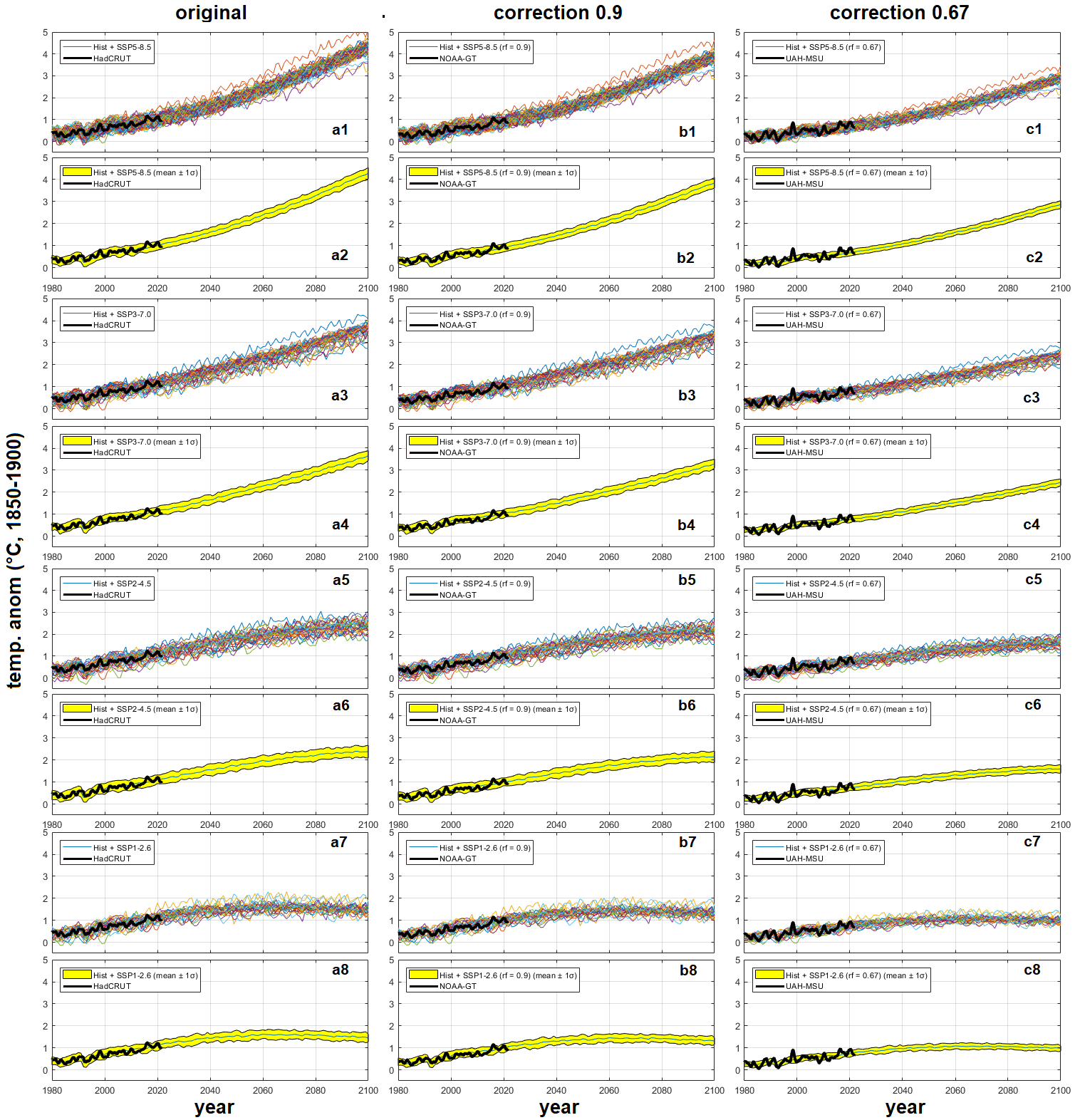
Figure 9: Low-ECS GCM simulations from 1980 to 2100 using historical + SSP1-2.6, SSP2-4.5, SSP3-7.0, and SSP5-8.5 scenarios: (a1-a8) original GCM simulations versus HadCRUT5; (b1-b8) GCM simulations reduced by 10% versus NOAAGlobalTemp v5; (c1-c8) GCM simulations reduced by 33% versus UAH-MSU-lt v6. The ordinates represent the temperature anomaly relative to the 1850-1900 average of the correspondent model set. The temperature records are baselined with the GCM simulations in 1980-1990.

		Hist + SSP1-2.6	Hist + SSP2-4.5	Hist + SSP3-7.0	Hist + SSP5-8.5
		(∘C)	(∘C)	(∘C)	(∘C)
Original	1980-1990	0.43 $\pm$ 0.19	0.43 $\pm$ 0.21	0.45 $\pm$ 0.20	0.37 $\pm$ 0.19
	2011-2021	1.01 $\pm$ 0.20	1.01 $\pm$ 0.22	1.05 $\pm$ 0.19	0.90 $\pm$ 0.21
	2040-2060	1.52 $\pm$ 0.21	1.75 $\pm$ 0.25	1.97 $\pm$ 0.21	1.98 $\pm$ 0.21
	2080-2100	1.52 $\pm$ 0.21	2.32 $\pm$ 0.25	3.28 $\pm$ 0.24	3.78 $\pm$ 0.24
RF = 0.90	1980-1990	0.39 $\pm$ 0.17	0.39 $\pm$ 0.19	0.41 $\pm$ 0.18	0.33 $\pm$ 0.17
	2011-2021	0.91 $\pm$ 0.18	0.91 $\pm$ 0.20	0.95 $\pm$ 0.17	0.81 $\pm$ 0.19
	2040-2060	1.37 $\pm$ 0.19	1.58 $\pm$ 0.23	1.77 $\pm$ 0.19	1.78 $\pm$ 0.19
	2080-2100	1.37 $\pm$ 0.19	2.09 $\pm$ 0.23	2.95 $\pm$ 0.22	3.40 $\pm$ 0.22
RF = 0.67	1980-1990	0.29 $\pm$ 0.13	0.29 $\pm$ 0.14	0.30 $\pm$ 0.13	0.25 $\pm$ 0.13
	2011-2021	0.68 $\pm$ 0.13	0.68 $\pm$ 0.15	0.70 $\pm$ 0.13	0.60 $\pm$ 0.14
	2040-2060	1.02 $\pm$ 0.14	1.17 $\pm$ 0.17	1.32 $\pm$ 0.14	1.33 $\pm$ 0.14
	2080-2100	1.02 $\pm$ 0.14	1.55 $\pm$ 0.17	2.20 $\pm$ 0.16	2.53 $\pm$ 0.16

Table 8: Low-ECS GCMs: global surface warming in the periods 1980-1990, 2011-2021, 2040-2060, and 2080-2100 using the simulations depicted in Figure 9. Original GCM simulations; (RF = 0.90) GCM simulations reduced by 10%; (RF = 0.67) GCM simulations reduced by 33%. The temperature anomaly is relative to the 1850-1900 average of the correspondent model set. The temperature records are baselined with the models simulations in 1980-1990.

5 Climate change expectations for the 21^st century

Climate impacts several areas of economic and environmental importance and its changes may require the implementation of various adaptation policies. However, climate change could also adversely affect some of the Earth’s climate systems such as in areas of water scarcity, coastal communities, natural ecosystems and others (IPCC, 2022). It is reasonable to assume that if climate change is too rapid and too significant, different areas could reach a point of vulnerability where adaptation will no longer be sufficient to avoid serious adverse effects. However, adaptation policies are much more affordable than mitigation ones, so the risks associated with possible future climate change should not be overestimated.

The IPCC (2021) used the GCM CMIP6 and various scenarios of global socioeconomic change predicted up to 2100 to produce hypothetical future stories on climate change for the 21^st century. Four SSP scenarios were studied here: the SSP1-2.6 (low GHG emissions in which CO₂ emissions are reduced to zero around 2075); SSP2-4.5 (intermediate GHG emissions in which CO₂ emissions increase around the current rate until 2050, and then decrease but not reach net zero by 2100); SSP3-7.0 (high GHG emissions where CO₂ emissions double by 2100); and SSP5-8.5 (very high GHG emissions where CO₂ emissions triple by 2075).

The IPCC (2022) states that if the global surface temperature rises significantly above 2^∘C over the next few decades compared to the pre-industrial period (1850-1900), adaptation policies may not be sufficient to reduce high risks related to climate change. Aggressive climate mitigation policies should therefore be implemented because the CMIP6 GCMs predict that the temperature will likely increase between 2°C and 3^∘C (compared to 1850-1900) by 2050 if anthropogenic greenhouse gas emissions are not significantly reduced as soon as possible.

However, in the previous sections we found that only the GCM group with low ECS, which is also the one predicting less warming, optimally reproduces the observed warming from 1980-1990 to 2011-2021 reported by the surface-based global temperature records. Therefore, its scenario forecasts for the 21^st century should be preferred for policy. Furthermore, we also found that global warming from 1980-1990 to 2011-2021 reported by the surface temperature records may need to be reduced on average by about 10% assuming that the ocean warming is correct and that the correct land/ocean temperature ratio is the one predicted by the models. Finally, if UAH-MSU-lt better reproduces the actual warming from 1980-1990 to 2011-2021, even the simulations of the low ECS GCMs would be running too hot and the warming they produce would need to be reduced by 33% to optimally accommodate the observations. Here, we show and discuss how the climate could change in the 21^st century under the above assumptions.

Figure 9 shows the simulations produced by the low ECS GCMs from 1980 to 2100 using the historical + SSP1-2.6, SSP2-4.5, SSP3-7.0, and SSP5-8.5 scenarios in three conditions: panels a1-a8 show the original GCM simulations versus HadCRUT5; panels b1-b8 show the GCM simulations reduced by 10% compared to NOAAGlobalTemp v5; and panels c1-c8 show the GCM simulations reduced by 33% compared to UAH-MSU-lt v6. The ordinates represent the temperature anomaly relative to the 1850-1900 average of the corresponding GCM set. The temperature records are baselined with the model simulations in 1980-1990. Table 8 reports the global surface warming forecasts produced by the low ECS GCMs in the periods 1980-1990, 2011-2021, 2040-2060 and 2080-2100 in the same three conditions.

The analysis shows that the expected warming of the low-ECS GCMs by 2040-2060 is close to 2^∘C also for the SSP3-7.0 and SSP5-8.5 scenarios, which Hausfather and Peters (2020) described as “unlikely” and as “highly unlikely”, respectively. However, if the surface temperature records contain a warming bias and, therefore, the GCM simulations need to be scaled down to better agree with the actual warming, the projected warming for 2040-2060 could be lower (or even significantly lower if UAH -MSU-lt v6 is correct) than 2^∘C also for the SSP3-7.0 and SSP5-8.5 scenarios.

There is indirect evidence that the surface-based temperature reconstructions could be affected by non-climatic warming biases. In fact, compared to the 1850-1900 mean, the average warming of 1980-1990 is 0.54^∘C for HadCRUT5 (infilled data), 0.48^∘C for GISTEMP v4 (using the period 1880-1900) and 0.47^∘C for NOAAGlobalTemp v5 (using the period 1880-1900). However, the low ECS GCMs give a slightly lower 1980-1990 warming, which is $0.41\pm 0.20$ ^∘C by averaging all GCM simulations although they better hindcast the 1980-2021 warming. In contrast, the medium and high ECS GCMs give $0.48\pm 0.27$ ^∘C and $0.47\pm 0.23$ ^∘C, respectively, which better fit the climate records; but then these same GCMs fail to hindcast the observed warming from 1980 to 2021.

The above findings suggest that climate change will likely be moderate over the next few decades and that adaptation policies should be sufficient to manage any adverse effects that may occur.

Furthermore, the warming hindcasted by the low-ECS models from 1850-1900 to 1980-1990 would be lower than $0.41\pm 0.20$ ^∘C if the climate simulations produced by them were to be scaled down. This evidence would suggest that the more recently applied homogenization adjustments to climate data to attempt to remove their non-climatic biases may have been inadequate and may have added or left spurious warming. For example,the continuous homogenization adjustments made to the surface-based temperature records during the last 10 years may have improperly cooled the raw temperature data of the past for many land stations (D’Aleo, 2016) and, simultaneously, may have improperly increased the warming trend from the 1970s to the present, and, in particular, that of the period 2000-2021 (Connolly et al., 2021; Scafetta, 2021a; Watts, 2022).

In fact, the scientific literature has indicated the period 2000-2014 as a “hiatus” or “pause” in global warming (IPCC, 2013) because all surface and satellite climate records available before 2014 (e.g. HadCRUT3, which was discontinued in 2014, Brohan et al. 2006) showed more than a decade of relatively little change. Later, however, new versions of the surface temperature records were published (e.g. HadCRUT4 and later HadCRUT5 non-infilled and infilled data) and the 2000-2014 “pause” has gradually disappeared because, from one climate version to the following one, it has been replaced by an increasingly strong warming trend; e.g. the trend was 0.03 °C/decade for HadCRUT3, 0.08 °C/decade for HadCRUT4, 0.10 °C/decade for HadCRUT5 non-infilled data, and 0.14 °C/decade for HadCRUT5 infilled data. See Figure 10 and Table 9. Yet, the 2000-2014 global warming “hiatus” is still visible in the UAH-MSU-lt v6 record, which shows a 2000-2014 warming trend of 0.012 °C/decade (Figure 2).

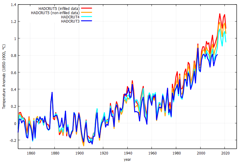
Figure 10: HadCRUT3 (1850-2014), HadCRUT4 (1850-2021), HadCRUT5 (non-infilled data, 1850-2021) and HadCRUT5 (filled data, 1850-2021) global surface temperature records relative to the 1850-1900 period.

	temperature anomaly (°C, 1850-1900)						trend (°C/year)
	1960-1980	1980-1990	1990-2000	2000-2010	2004-2014	2011-2021	2000-2014	2000-2021
HadCRUT5 (infilled data)	0.28	0.53	0.68	0.89	0.94	1.12	0.014	0.022
HadCRUT5 (non infilled data)	0.24	0.49	0.65	0.83	0.87	1.04	0.010	0.019
HadCRUT4	0.25	0.42	0.59	0.78	0.81	0.95	0.008	0.016
HadCRUT3	0.24	0.43	0.58	0.76	0.76		0.003

Table 9: Warming means and trends in various periods for HadCRUT3 (1850-2014), HadCRUT4 (1850-2021), HadCRUT5 (non-infilled data, 1850-2021) and HadCRUT5 (filled data, 1850-2021) global surface temperature records. See Figure 10.

6 Conclusion

Here I tested how well the CMIP6 GCMs – grouped into low, medium and high ECS subgroups – hindcast the global surface temperature warming from 1980-1990 to 2011-2021 reported by four surface temperature records (ERA5-T2m, HadCRUT5, GISTEMP v4, and NOAAGlobTemp v5) and by the satellite-based UAH-MSU-lt v6 temperature record. The latter was used as the lowest possible estimate for the global surface temperature warming during the analyzed period. The rationale for adding a comparison with the lower troposphere temperature record is that surface temperatures could be affected by significant non-climatic warming bias due, for example, to poorly corrected urban heats and many other factors (Connolly et al., 2021; D’Aleo, 2016; Scafetta, 2021a; Watts, 2022). For example, indirect evidence for a significant warming bias, especially over land, may be also provided by the so-called "Divergence Problem" that is the apparent decoupling between three ring width chronologies and the rising temperature measurements starting from the 1970s (Büntgen et al., 2021; Esper et al., 2018; Scafetta, 2021a).

Using the 143 GCM mean simulations available for four different SSPs, all medium and high ECS models turn out to be warmer than observations. Using the 688 CMIP6 ensemble member simulations available, 94% to 100% of the simulations produced by GCMs with medium and high ECS hindcasted greater warming than the five temperature records. In contrast, the low-ECS models are statistically distributed around the observed warming values obtained from the four surface-based temperature records. However, if the UAH-MSU-LT record better represents the actual 2011-2021 warming, even the low-ECS GCM group would produce on average too hot hindcasts.

I also tested whether the internal variability of the models could produce results distributed around the observations. Its effect was modeled using three fixed precision options. Assuming high ($\sigma_{H}\approx 0.05$^∘C) and medium ($\sigma_{M}\approx 0.10$^∘C) precision, it was found that 98-100% and 92 -98%, respectively, of all possible outputs from the medium and high ECS GCMs would be warmer than observations. Only the theoretical results produced by the low-ECS GCM group optimally agree with the surface-based temperature records. If the required model accuracy is quite low ($\sigma_{L}\approx 0.15$ ^∘C), the middle and high GCM simulation groups would agree better with the data, but this agreement could still be quite unsatisfactory because 87% to 93% (which is still well outside the $\pm 1$$\sigma$ or 68% confidence interval) of their hindcasts would still be too hot. In any case, the low precision option should be considered very unsatisfactory because it would allow the GCMs to deviate too much from the observations. Moreover, such poor precision would not seem consistent with the natural variability of the data as argued in Appendix B. Figure 5 suggests that such a low precision could only occur for EC-Earth3 GCM.

Figures 5 and 6 also show that very few GCMs with medium and high ECS could produce some simulations consistent with the actual temperature values. In particular, the two high-ECS CNRM models (Séférian et al., 2019; Voldoire et al., 2019) appear to perform better than the other models of the same group. However, as a group, the high-ECS models are physically incompatible with the low-ECS ones. Indeed, the internal parameters of the GCMs are carefully tuned to obtain results as acceptable as possible (Hourdin et al., 2017; Mauritsen et al., 2019). Therefore, the good performance of some isolated cases could hardly be used to validate the corresponding model since the tuning operations also risk masking fundamental physical problems and, therefore, the need for model and/or forcing improvements.

It was found that only the low-ECS GCM group agrees optimally with the surface-based temperature records because their full hindcast range well encompasses the actual temperature warming values  from 1980-1990 to 2011-2021. Therefore, since the three ECS chosen ranges should be considered large enough to be incompatible with each other, the GCM group with low ECS should be preferred to the other two, implying that the most likely ECS should be equal to or lower than 3^∘C. This result confirms Scafetta (2022). In fact, the performance of the models seems to increase as the ECS decreases (Scafetta, 2021b).

However, the actual ECS could also be significantly lower than 3^∘C if the UAH-MSU-lt record better represents the 2011-2021 surface warming. In fact, the satellite record shows that from 1980-1990 and 2011-2021 the global surface temperature may have warmed by about 0.40^∘C, which is about 30% less than 0.58^∘C as reported by ERA5-T2m, HadCRUT5, and GISTEMP v4. In this case, even the GCM group with low ECS would show poor accuracy in reproducing the temperature data because their average hindcast is about 0.60^∘C. This means that the actual ECS could also be 33% lower than that which characterizes the low ECS GCM group: that is, it could need to be reduces from 1.8-3.0^∘C to 1.2-2.0^∘C. This conclusion cannot be ruled out because: (1) the surface temperature records appear to be severely affected by non-climatic warming bias (Connolly et al., 2021; D’Aleo, 2016; Scafetta, 2021a; Watts, 2022), as the direct comparison between land and ocean warming proposed here also seeems to confirm (Figure 8); (2) because a number of independent studies have concluded that the ECS could be within such a low range (e.g.: Lewis and Curry, 2018; Lindzen and Choi, 2011; Scafetta, 2013; Stefani, 2021; van Wijngaarden and Happer, 2020).

There is a third possibility which would also imply that the actual ECS should be relatively low. The climate system, in fact, appears to be also modulated by multidecennial and millennial natural oscillations such as those related to solar forcings and other astronomical ones, which are not reproduced by the GCMs (cf.: Scafetta, 2013, 2021c; Wyatt and Curry, 2014). Their presence implies that the ECS of GCMs should be at least halved (cf.: Loehle and Scafetta, 2011; Scafetta, 2012a, 2021c) and could vary approximately between 1.0^∘C and 2.5^∘C, as found by several independent studies (cf.: Lewis and Curry, 2018; Lindzen and Choi, 2011; Scafetta, 2013; Stefani, 2021; van Wijngaarden and Happer, 2020). If so, future climate warming and changes will be moderate and naturally oscillating (Scafetta, 2013, 2021c) and the rate of global surface warming should likely remain quite low until 2030-2040, when solar activity is expected to increase again due to its natural multi-decadal oscillations (Scafetta, 2012b; Scafetta and Bianchini, 2022, and several others).

In any case, even remaining within the theoretical framework of the CMIP6 GCMs, it should be concluded that only the low ECS GCM group can be considered sufficiently validated by the global surface warming observed from 1980-1990 to 2011-2021. Therefore, only the 21^st century climate projections produced by the low ECS GCMs should be used for policy. For decades to come, these models predict more moderate warming than the GCM groups with medium and high ECS do for similar greenhouse gas emission scenarios. By 2050, projected warming is expected to be around 2^∘C or less even for the worst greenhouse gas emission scenarios. This moderate warming should not be considered particularly alarming because the impact and risk assessments related to it are considered “moderate” assuming even low to no adaptation (IPCC, 2022). Furthermore, as surface-based temperature records are likely affected by warming biases and are characterized by natural oscillations that are not reproduced by the CMIP6 models, the global warming expected for the next few decades may be even more moderate than predicted by the low-ECS GCMs and could easily fall within a safe temperature range where climate adaptation policies will suffice. Therefore, aggressive mitigation policies aimed at rapidly and drastically reducing GHG emissions in order to avoid a too rapid rise in temperature do not seem justified, also because their costs seem to outweigh any realistic benefits (cf. Bezdek et al., 2019).

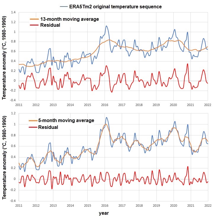
Figure 11: Possible decomposition of the ERA5-T2m global surface temperature record (blue) into a signal (orange, made of 13 and 5 month moving averages) and a residual-noise (red) record that could be used to evaluate the error of the mean.

Appendix A: Evaluation of the error of the mean for temperature records

Computer simulations are made of pure numbers and their averages over a given period of time are error free. The uncertainty associated with their unforced internal variability is a different matter and will be discussed in Appendix B.

Conversely, the data points of the temperature records are affected by small statistical errors, which however are not always readily available as is the case with the ERA5-T2m record. Let’s address the issue.

A generic time series $y_{t}$ with $t=1,...,N$ could be affected by Gaussian distributed uncertainties $\xi_{t}$ with zero mean and standard deviation $\sigma_{\xi}$ as

$$y_{t}=x_{t}+\xi_{t},$$ (3)

where $x_{t}$ is the physical signal of the record. Its mean is

$$\bar{y}=\frac{1}{N}\sum_{t=1}^{N}y_{t}\pm\sigma_{\xi}/\sqrt{N},$$ (4)

where $\bar{\sigma}=\sigma_{\xi}/\sqrt{N}$ is the error of the mean.

It is important to note that $\sigma_{\xi}$ is the standard error of the uncertainties $\xi_{t}$, not that of the signal $y_{t}$. For example, the ERA5-T2m 2011-2021 average (baselined to 1980-1990) is 0.578^∘C, which was obtained by integrating on the globe the temperature variations that occurred in each cell of the surface grid worldwide. The standard deviation of the same record is $\sigma_{y,month}=0.20$^∘C using the monthly record and $\sigma_{y,year}=0.18$^∘C using the annual record. For random variables, the error of the mean does not depend on the time resolution of the record, that is, the monthly and yearly resolved records should give $\bar{\sigma}_{year}=\bar{\sigma}_{month}$. However, if we apply the equation $\bar{\sigma}=\sigma_{y}/\sqrt{N}$ from 2011 to 2021, for ERA5-T2m we get $\bar{\sigma}_{year}=0.054$^∘C (using N=11 points) and $\bar{\sigma}_{month}=0.017$^∘C (using N=132 points), respectively. This shows that from 2011 to 2021 the ERA-T2m record is not composed of random variables floating around an average value, but contains a physical signal.

It can be assumed that the physical signal of ERA5-T2m is represented by the moving averages of the data at 13 months, 5 months or 3 months while the residuals are the noise components that should be used to evaluate $\sigma_{\xi}$ and $\bar{\sigma}=\sigma_{\xi}/\sqrt{N}$. The three choices give $\bar{\sigma}=0.01$^∘C, $\bar{\sigma}=0.006$^∘C, and $\bar{\sigma}=0.005$^∘C, respectively, which suggest that the actual error of the 2011-2021 mean could be $\bar{\sigma}=0.01$^∘C or probably less. The first two examples of data decomposition are shown in Figure 11.

Alternatively, the statistical uncertainty associated with ERA5-T2m could be considered compatible with those explicitly provided by the other available global surface temperature records. In the case of the GISTEMP record, Lenssen et al. (2019) calculated that the resulting 95% uncertainties are near $\bar{\sigma}_{95\%,annual}\approx 0.05$ ^∘C in the global annual mean for the last 50 years. HadCRUT5’s global surface temperature record includes its 95% confidence interval estimate and, from 2011 to 2021, the uncertainties for the monthly and annual averages are $\bar{\sigma}_{95\%,monthly}\approx 0.05$^∘C and $\bar{\sigma}_{95\%,annual}\approx 0.03$^∘C, respectively. Berkeley Earth land/ocean temperature record estimates $\bar{\sigma}_{95\%,monthly}\approx 0.042$ ^∘C, $\bar{\sigma}_{95\%,annual}\approx 0.028$^∘C, and $\bar{\sigma}_{95\%,decadal}\approx 0.022$^∘C during the same period. Note that the error of the mean must decrease as the time scale increases.

Therefore, adopting the equation $\bar{\sigma}_{95\%}=1.96\times\sigma_{\xi}/\sqrt{N}$, the probable error for the 2011-2021 mean could be of about 0.01^∘C or even smaller. In fact, using the above estimates, we obtain: $0.05/\sqrt{11}=0.015$^∘C, $0.05/\sqrt{132}=0.0043$^∘C, $0.03/\sqrt{11}=0.009$^∘C, $0.042/\sqrt{132}=0.004$^∘C, and $0.028/\sqrt{11}=0.008$^∘C respectively, the mean of which is approximately 0.008^∘C. Alternatively, the 95% uncertainty over the period 2011-2021 cannot be greater than about $\pm$0.02^∘C, as explicitly reported by the Berkeley Earth land/ocean temperature record for the ten-year scale.

Therefore, various methodologies suggest that the uncertainty of the temperature means in the 11-year period from 2011 to 2021 is very small, around $\pm 0.01$^∘C at 95% confidence and can be safely ignored as done for example in Scafetta (2022).

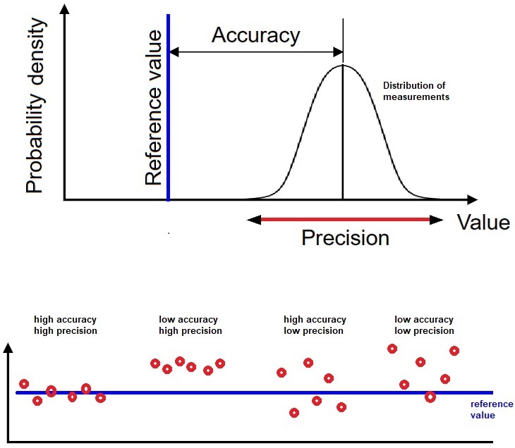
Figure 12: Definition of accuracy and precision, and examples of high and low accuracy and precision cases where the red dots are ensembles of measurements.

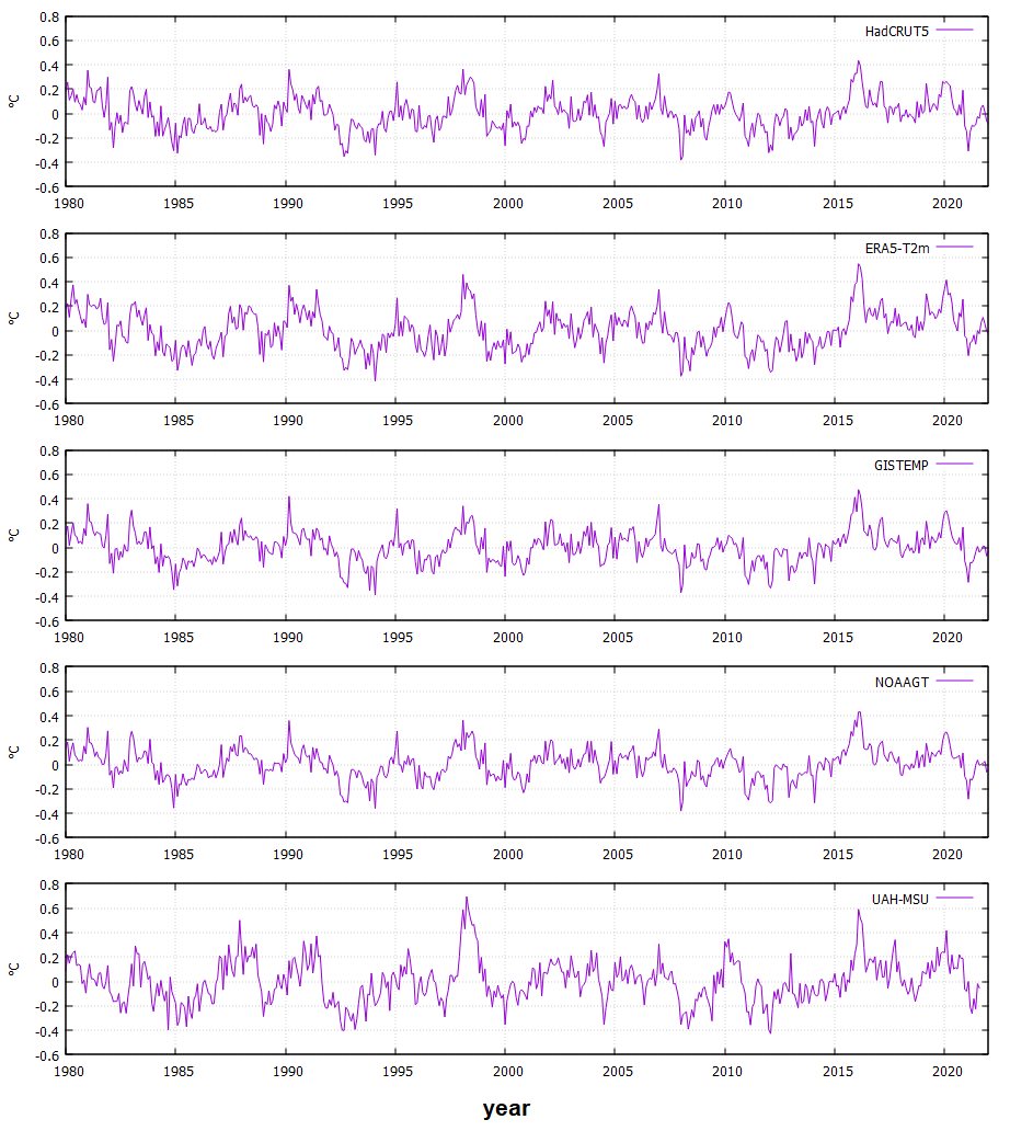
Figure 13: 15-year high-pass filter of HadCRUT5, ERA5-T2m, GISTEMP v4, NOAAGlobTemp v5, and UAH-MSU-lt v6 temperature records.

Appendix B: Provisional assessment of an acceptable internal variability of the models

Climate models are unable to accurately simulate temperature records due to various uncertainties. For example, only by varying the initial conditions different climatic trajectories are obtained which evolve around an ideal average with a certain variance.

Each GCM is characterized by its own internal variability. However, in the main text, we argued that such uncertainty could not be arbitrarily large because the models must be both accurate and precise. Figure 12 explains the concepts of “accuracy”, which measures the proximity of the model hindcasts to the real value, and of “precision”, which indicates the proximity of the same hindcasts to each other.

An acceptable range for the distribution of hindcasts related to the internal variability of the models could be assessed by observing that temperature fluctuations at time scales lower than, for example, 15 years, (which include the climatic oscillations of the ENSO and those of the 11-year solar cycle) may not be adequately predicted by the models. From the point of view of the models, the temperature fluctuations at those time scales could be considered stochastic and their standard deviation from the mean could represent the acceptable range that can be associated with the unforced internal variability of the models (cf. Knight et al., 2009).

Figure 13 shows the 15-year high-pass filter curves of HadCRUT5, ERA5-T2m, GISTEMP v4, NOAAGlobTemp v5, and UAH-MSU-lt v6 temperature records from 1980 to 2021. Using the standard deviation $\sigma$ for each record, the error of the mean on 11-year intervals (e.g. from 2011 to 2021) at the 95% confidence is $\bar{\sigma}_{95\%}=1.96\times\sigma/\sqrt{11}$, that is: $\bar{\sigma}_{95\%}=0.080$^∘C for HadCRUT5; $\bar{\sigma}_{95\%}=0.094$^∘C for ERA5-T2m; $\bar{\sigma}_{95\%}=0.079$^∘C for GISTEMP v4; $\bar{\sigma}_{95\%}=0.075$^∘C for GISTEMP v4; and $\bar{\sigma}_{95\%}=0.104$^∘C for UAH-MSU-lt v6.

Based on the above assumptions, over an 11-year period, the uncertainty of the 2011-2021 warming compared to 1980-1990 could be estimated at approximately $\pm 0.1$^∘C at the 95% confidence, which corresponds to the high precision option ($\sigma_{H}=0.05$^∘C) discussed in Section 3.

The high precision option should not be interpreted as the actual dispersion produced by each GCM, which varies greatly from model to model, but only as the acceptable uncertainty that a CGM should exhibit in reproducing the warming from 1980-1990 to 2011-2021. In our case, a $\pm 0.1$^∘C error would imply a $\pm 0.17\%$ of the actual warming from 1980 to 2021, which can be considered a reasonable error.

Conflict of Interest

The author declares no conflict of interest.

Data Availability Statement

All data used in the manuscript can be downloaded from KNMI Climate Explorer or from the original websites:

• KNMI Climate Explorer, https://climexp.knmi.nl/start.cgi

• ERA5-T2m, https://cds.climate.copernicus.eu/cdsapp#!/dataset/reanalysis-era5-single-levels-monthly-means

• GISTEMP v4, https://data.giss.nasa.gov/gistemp, https://data.giss.nasa.gov/gistemp/graphs_v4/

• HadCRUT5, https://www.metoffice.gov.uk/hadobs/hadcrut5/

• HadCRUT4, https://www.metoffice.gov.uk/hadobs/hadcrut4/

• HadCRUT3, https://www.metoffice.gov.uk/hadobs/hadcrut3/

• NOAAGlobTemp v5, https://www.eea.europa.eu/data-and-maps/data/external/noaa-global-temperature-v5

• Berkeley Earth land/ocean temperature, http://berkeleyearth.org/archive/land-and-ocean-data/

• Japanese Meteorological Agency, https://ds.data.jma.go.jp/tcc/tcc/products/gwp/temp/ann_wld.html

• UAH-MSU-lt v6, https://www.nsstc.uah.edu/data/msu/v6.0/tlt/uahncdc_lt_6.0.txt

• CMIP6 GCMs, http://climexp.knmi.nl/selectfield_cmip6.cgi?id=someone@somewhere.

References

- Bezdek et al. (2019) Bezdek, R., Idso, C. D., Legates, D., Singer, S. F. (2019). Climate Change Reconsidered II: Fossil Fuels. Nongovernmental International Panel on Climate Change (NIPCC). The Heartland Institute. http://climatechangereconsidered.org/climate-change-reconsidered-ii-fossil-fuels/
- Brohan et al. (2006) Brohan, P., Kennedy, J.J., Harris, I., Tett, S.F.B., Jones, P.D. (2006) Uncertainty estimates in regional and global observed temperature changes: a new dataset from 1850. J. Geophys. Res, 111, D12106. https://doi.org/10.1029/2005JD006548.
- Büntgen et al. (2021) Büntgen, U., Allen, K., Anchukaitis, K.J. et al. The influence of decision-making in tree ring-based climate reconstructions. Nature Communication 12, 3411 (2021). https://doi.org/10.1038/s41467-021-23627-6
- Christy et al. (2018) Christy, J.R., Spencer, R.W., Braswell, W.D., Junod, R. (2018). Examination of space-based bulk atmospheric temperatures for climate research. Int. J. Remote Sens. 39, 3580–3607. https://doi.org/10.1080/01431161.2018.1444293
- Connolly et al. (2021) Connolly, R., Soon, W., Connolly, et al. (2021). How much has the Sun influenced Northern hemisphere temperature trends? An ongoing debate. Research in Astronomy and Astrophysics, 21, 131. https://doi.org/10.1088/1674-4527/21/6/131
- D’Aleo (2016) D’Aleo, J.S. (2016). A critical look at surface temperature records. In Easterbrook, D.J.: Evidence-Based Climate Science (Second Edition), pp. 11–48, Elsevier. https://doi.org/10.1016/B978-0-12-804588-6.00002-1
- Esper et al. (2018) Esper, J., George S. St., Anchukaitis K., D’Arrigo R., Ljungqvist F.C., Luterbacher J., Schneider L., Stoffel M., Wilson R., Büntgen U. (2018). Large-scale, millennial-length temperature reconstructions from tree-rings. Dendrochronologia 50, 81–90. https://doi.org/10.1016/j.dendro.2018.06.001
- Eyring et al. (2016) Eyring, V., Bony, S., Meehl, G.A., et al. (2016). Overview of the Coupled Model Intercomparison Project Phase 6 (CMIP6) experimental design and organization. Geoscientific Model Development, 9 (5), 1937–1958. https://doi.org/10.5194/gmd-9-1937-2016
- Grose et al. (2017) Grose, M.R., Colman, R., Bhend, J. et al. (2017). Limits to global and Australian temperature change this century based on expert judgment of climate sensitivity. Climate Dynamics 48, 3325–3339. https://doi.org/10.1007/s00382-016-3269-2
- Hausfather and Peters (2020) Hausfather, Z., Peters, G. P. (2020). Emissions – the ’business as usual’ story is misleading. Nature 577 (618–620). https://doi.org/10.1038/d41586-020-00177-3
- Heo et al. (2014) Heo, K.-Y., Ha, K.-J., Yun, K.-S., Lee, S.-S., Kim, H.-J., Wang, B. (2014), Methods for uncertainty assessment of climate models and model predictions over East Asia. Int. J. Climatology, 34: 377–390. https://doi.org/10.1002/joc.3692
- Hersbach et al. (2020) Hersbach, H., Bell, B., Berrisford, P., et al. (2020). The ERA5 global reanalysis. Quaternary Journal of the Royal Meteorological Society 146, 1999–2049. https://doi.org/10.1002/qj.3803
- Hourdin et al. (2017) Hourdin, F., Mauritsen, T., Gettelman, A., Golaz, J., Balaji, V., Duan, Q., Folini, D., Ji, D., Klocke, D., Qian, Y., Rauser, F., Rio, C., Tomassini, L., Watanabe, M., and Williamson, D. (2017). The Art and Science of Climate Model Tuning. Bulletin of the American Meteorological Society 98, 3, 589–602. https://doi.org/10.1175/BAMS-D-15-00135.1
- Huntingford et al. (2020) Huntingford, C., Williamson, M.S., Nijsse, F.J.M.M (2020). CMIP6 climate models imply high committed warming. Climatic Change 162, 1515–1520. https://doi.org/10.1007/s10584-020-02849-5
- Knight et al. (2009) Knight, J., Kenned, J.J., Folland, C., Harris, G., Jones, G.S., Palmer, M., Parke, D., Scaife, A., Stott, P. (2009). Do global temperature trends over the last decade falsify climate predictions? In “State of the Climate in 2008”. Bull. Am. Meteorol. Soc. 90 (8) (S1–S196).
- Knutti et al. (2017) Knutti, R., Rugenstein, M. A., & Hegerl, G. C. (2017). Beyond equilibrium climate sensitivity. Nature Geoscience, 10, 727–736. https://doi.org/10.1038/ngeo3017
- IPCC (2013) IPCC (2013). Climate Change 2013: The Physical Science Basis. Contribution of Working Group I to the Sixth Assessment Report of the Intergovernmental Panel on Climate Change. Cambridge (UK): Cambridge University Press.. Retrieved from https://www.ipcc.ch/assessment-report/ar5/
- IPCC (2021) IPCC (2021). Climate Change 2021: The Physical Science Basis. Contribution of Working Group I to the Sixth Assessment Report of the Intergovernmental Panel on Climate Change. Cambridge (UK): Cambridge University Press. Retrieved from https://report.ipcc.ch/ar6wg1/
- IPCC (2022) IPCC (2022). Climate Change 2022: Impacts, Adaptation and Vulnerability. Contribution of Working Group II to the Sixth Assessment Report of the Intergovernmental Panel on Climate Change. Cambridge (UK): Cambridge University Press. Retrieved from https://report.ipcc.ch/ar6wg2/
- Ishihara (2006) Ishihara, K. (2006). Calculation of global surface temperature anomalies with COBE-SST. Weather Service Bulletin,73, S19–S25.
- Lenssen et al. (2019) Lenssen, N. J. L., Schmidt, G. A., Hansen, J. E., Menne, M. J., Persin, A., Ruedy, R., Zyss, D. (2019). Improvements in the GISTEMP uncertainty model. Journal of Geophysical Research: Atmospheres, 124, 6307– 6326. https://doi.org/10.1029/2018JD029522
- Lewis and Curry (2018) Lewis, N., & Curry, J. (2018). The impact of recent forcing and ocean heat uptake data on estimates of climate sensitivity. Journal of Climate, 31, 6051–6071. https://doi.org/10.1175/JCLI-D-17-0667.1
- Lindzen and Choi (2011) Lindzen, R. S., & Choi, Y.-S. (2011). On the observational determination of climate sensitivity and its implications. Asia-Pacific Journal of Atmospheric Sciences, 47, 377–390. https://doi.org/10.1007/s13143-011-0023-x
- Loehle and Scafetta (2011) Loehle, C., Scafetta, N. (2011). Climate Change Attribution Using Empirical Decomposition of Climatic Data. The Open Atmospheric Science Journal, 5, 74–86. https://doi.org/10.2174/1874282301105010074
- Fu et al. (2011) Fu, Q., Manabe, S., and Johanson, C. M. (2011). On the warming in the tropical upper troposphere: Models versus observations. Geophys. Res. Lett. 38, L15704, https://doi.org/10.1029/2011GL048101
- Mauritsen et al. (2019) Mauritsen, T., Bader, J., Becker, T., Behrens, J., Bittner, M., Brokopf, R., et al. (2019). Developments in the MPI-M Earth System Model version 1.2 (MPI-ESM1.2) and its response to increasing CO2. Journal of Advances in Modeling Earth Systems, 11, 998–1038. https://doi.org/10.1029/2018MS001400
- McKitrick and Christy (2018) McKitrick, R., Christy, J. (2018). A test of the tropical 200 to 300 hPa warming rate in climate models. Earth and Space Science 5, 529–536. https://doi.org/10.1029/2018EA000401
- McKitrick and Christy (2020) McKitrick, R., Christy, J. (2020). Pervasive warming bias in CMIP6 tropospheric layers. Earth and Space Science 7, e2020EA001281. https://doi.org/10.1029/2020EA001281
- Mears and Wentz (2016) Mears, C. A., & Wentz, F. J. (2016). Sensitivity of satellite-derived tropospheric temperature trends to the diurnal cycle adjustment. Journal of Climate, 29, 3629–3646. https://doi.org/10.1175/jcli-d-15-0744.1
- Meehl et al. (2011) Meehl, G., Arblaster, J., Fasullo, J. et al. (2011). Model-based evidence of deep-ocean heat uptake during surface-temperature hiatus periods. Nature Clim Change 1, 360–364. https://doi.org/10.1038/nclimate1229
- Mitchell et al. (2020) Mitchell, D.M., Lo, Y.T.E., Seviour, W.J.M., Haimberger, L., Polvani, L.M. (2020). The vertical profile of recent tropical temperature trends: Persistent model biases in the context of internal variability. Environ. Res. Lett. 15, 1040b4. https://doi.org/10.1088/1748-9326/ab9af7
- Möller (1963) Möller, F. (1963). On the influence of changes in the CO2 concentration in air on the radiation balance of the Earth’s surface and on the climate. Journal of Geophysical Research, 68, 3877– 3886. https://doi.org/10.1029/jz068i013p03877
- Morice et al. (2012) Morice, C. P., Kennedy, J. J., Rayner, N. A., Jones, P. D. (2012). Quantifying uncertainties in global and regional temperature change using an ensemble of observational estimates: The HadCRUT4 dataset, J. Geophys. Res., 117, D08101. https://doi.org/10.1029/2011JD017187
- Morice et al. (2021) Morice, C. P., Kennedy, J. J., Rayner, N. A., et al. (2021). An updated assessment of near-surface temperature change from 1850: the HadCRUT5 data set. Journal of Geophysical Research: Atmospheres, 126, e2019JD032361. https://doi.org/10.1029/2019JD032361
- Nijsse et al. (2020) Nijsse, F. J. M. M., Cox, P. M., and Williamson, M. S. (2020). Emergent constraints on transient climate response (TCR) and equilibrium climate sensitivity (ECS) from historical warming in CMIP5 and CMIP6 models. Earth Syst. Dynam., 11, 737–750, https://doi.org/10.5194/esd-11-737-2020.
- Oldenborgh (2020) van Oldenborgh, G. J. (2020). The KNMI climate explorer. © 2020 KNMI (results, code)/World Meteorological organization (WMO) (design). Retrieved from https://climexp.knmi.nl/start.cgi
- Scafetta and Ouyang (2019) Scafetta N., Ouyang S. (2019). Detection of UHI bias in China climate network using Tmin and Tmax surface temperature divergence. Global Planet Change 181, 102989. https://doi.org/10.1016/j.gloplacha.2019.102989
- Rohde and Hausfather (2020) Rohde, R. A., Hausfather, Z. (2020). The Berkeley Earth Land/Ocean Temperature Record. Earth Syst. Sci. Data, 12, 3469–3479. https://doi.org/10.5194/essd-12-3469-2020, 2020
- Ribes et al. (2021) Ribes, A., Qasmi, S., & Gillett, N. P. (2021). Making climate projections conditional on historical observations. Science Advances, 7 (4), eabc0671. https://doi.org/10.1126/sciadv.abc0671
- Scafetta (2012a) Scafetta, N. (2012a). Testing an astronomically based decadal-scale empirical harmonic climate model versus the IPCC (2007) general circulation climate models. J. Atmos. Solar-Terrestrial Phys. 80 124–137. https://doi.org/10.1016/j.jastp.2011.12.005
- Scafetta (2012b) Scafetta, N. (2012b). Multi-scale Harmonic Model for Solar and Climate Cyclical Variation throughout the Holocene Based on Jupiter-Saturn Tidal Frequencies Plus the 11-year Solar Dynamo Cycle. J. Atmos. Solar-Terrestrial Phys. 80, 296–311. https://doi.org/10.1016/j.jastp.2010.04.015
- Scafetta (2013) Scafetta, N. (2013). Discussion on climate oscillations: CMIP5 general circulation models versus a semiempirical harmonic model based on astronomical cycles. Earth-Science Reviews, 126, 321–357. https://doi.org/10.1016/j.earscirev.2013.08.008
- Scafetta (2021a) Scafetta, N. (2021a). Detection of non-climatic biases in land surface temperature records by comparing climatic data and their model simulations. Climate Dynamics, 56, 2959–2982. https://doi.org/10.1007/s00382-021-05626-x
- Scafetta (2021b) Scafetta, N. (2021b). Testing the CMIP6 GCM simulations versus surface temperature records from 1980–1990 to 2011–2021: High ECS is not supported. Climate, 9(11), 161. https://doi.org/10.3390/cli9110161
- Scafetta (2021c) Scafetta, N. (2021c). Reconstruction of the Interannual to Millennial Scale Patterns of the Global Surface Temperature. Atmosphere, 12, 147. https://doi.org/10.3390/atmos12020147
- Scafetta (2022) Scafetta, N. (2022). Advanced testing of low, medium, and high ECS CMIP6 GCM simulations versus ERA5-T2m. Geophysical Research Letters, 49, e2022GL097716. https://doi.org/10.1029/2022GL097716
- Scafetta and Bianchini (2022) Scafetta, N., Bianchini, A. (2022). The Planetary Theory of Solar Activity Variability: A Review. Front. Astron. Space Sci., 9:937930. https://doi.org/10.3389/fspas.2022.937930
- Séférian et al. (2019) Séférian, R., Nabat, P., Michou, M., Saint-Martin, D., Voldoire, A., Colin, J., et al. (2019). Evaluation of CNRM Earth-System model, CNRM-ESM2-1: role of Earth system processes in present-day and future climate. Journal of Advances in Modeling Earth Systems, 11, 4182–4227. https://doi.org/10.1029/2019MS001791
- Seo et al. (2018) Seo, Y.-W., Yun, K.-S., Lee, J.-Y., Lee, Y.-W., Ha, K.-J., Jhun, J.-G. (2018). Future changes due to model biases in probabilities of extreme temperatures over East Asia using CMIP5 data. Int. J. Climatology, 38: 1177–1188. https://doi.org/10.1002/joc.5233
- Simmons et al. (2021) Simmons, A., Hersbach, H., Munoz Sabater, J., et al. (2021). Low frequency variability and trends in surface air temperature and humidity from ERA5 and other datasets. ECMWF. https://doi.org/10.21957/LY5VBTBFD
- Spencer et al. (2017) Spencer, R. W., Christy, J. R., & Braswell, W. D. (2017). UAH Version 6 global satellite temperature products: Methodology and results. Asia-Pacific Journal of Atmospheric Sciences, 53, 121– 130. https://doi.org/10.1007/s13143-017-0010-y
- Stefani (2021) Stefani, F. (2021). Solar and anthropogenic influences on climate: Regression analysis and tentative predictions. Climate, 9, 163. https://doi.org/10.3390/cli9110163
- Tokarska et al. (2020) Tokarska, K. B., Stolpe, M. B., Sippel, S., et al. (2020). Past warming trend constrains future warming in CMIP6 models. Science Advances, 6 (12). https://doi.org/10.1126/sciadv.aaz9549
- Voldoire et al. (2019) Voldoire, A., Saint-Martin, D., Sénési, S., Decharme, B., Alias, A., Chevallier, M., et al. (2019). Evaluation of CMIP6 DECK experiments with CNRM-CM6-1. Journal of Advances in Modeling Earth Systems, 11, 2177–2213. https://doi.org/10.1029/2019MS001683
- Voosen (2019) Voosen, P. (2019). New climate models predict a warming surge: Scientists question whether stronger anticipated response to greenhouse gases is realistic. Science. https://doi.org/10.1126/science.aax7217
- Watts (2022) Watts, A. (2022). Corrupted climate stations: The official U.S. temperature record remains fatally flawed. The Heartland Institute. https://www.heartland.org/_template-assets/documents/publications/2022_Surface_Station_Report.pdf
- Wigley et al. (1997) Wigley, T. M. L., Jones, P. D., Raper, S. C. B. (1997). The observed global warming record: What does it tell us? PNAS 94 (16) 8314-8320. https://doi.org/10.1073/pnas.94.16.8314
- van Wijngaarden and Happer (2020) van Wijngaarden, W. A., & Happer, W. (2020). Dependence of Earth’s thermal radiation on five most abundant greenhouse gases (pp. 1–38). Cornell University. Retrieved from https://arxiv.org/abs/2006.03098
- Wyatt and Curry (2014) Wyatt, M., Curry, J. (2014). Role of Eurasian Arctic shelf sea ice in a secularly varying hemispheric climate signal during the 20th century. Climate Dynamics 42, 2763–2782. https://doi.org/10.1007/s00382-013-1950-2
- Zelinka et al. (2020) Zelinka, M. D., Myers, T. A., McCoy, D. T., et al. (2020). Causes of higher climate sensitivity in CMIP6 models. Geophysical Research Letters, 47, e2019GL085782. https://doi.org/10.1029/2019gl085782
- Zhang et al. (2019) Zhang, H.-M., Lawrimore, J. H.,Huang, B., Menne, M. J.,Yin, X., Sánchez-Lugo, A., Gleason, B. E., Vose, R., Arndt, D., Rennie, J. J., Williams, C. N. (2019). Updated temperature data give a sharper view of climate trends, Eos, 100. https://doi.org/10.1029/2019EO128229.
- Zhu et al. (2020) Zhu, J., Poulsen, C. J., & Otto-Bliesner, B. L. (2020). High climate sensitivity in CMIP6 model not supported by paleoclimate. Nature Climate Change, 10, 378–379. https://doi.org/10.1038/s41558-020-0764-6