Multibody molecular docking on a quantum annealer

Abstract

Molecular docking, which aims to find the most stable interacting configuration of a set of molecules, is of critical importance to drug discovery. Although a considerable number of classical algorithms have been developed to carry out molecular docking, most focus on the limiting case of docking two molecules. Since the number of possible configurations of $N$ molecules is exponential in $N$, those exceptions which permit docking of more than two molecules scale poorly, requiring exponential resources to find high-quality solutions. Here, we introduce a one-hot encoded quadratic unconstrained binary optimization formulation (QUBO) of the multibody molecular docking problem, which is suitable for solution by quantum annealer. Our approach involves a classical pre-computation of pairwise interactions, which scales only quadratically in the number of bodies while permitting well-vetted scoring functions like the Rosetta REF2015 energy function to be used. In a second step, we use the quantum annealer to sample low-energy docked configurations efficiently, considering all possible docked configurations simultaneously through quantum superposition. We show that we are able to minimize the time needed to find diverse low-energy docked configurations by tuning the strength of the penalty used to enforce the one-hot encoding, demonstrating a 3-4 fold improvement in solution quality and diversity over performance achieved with conventional penalty strengths. By mapping the configurational search to a form compatible with current- and future-generation quantum annealers, this work provides an alternative means of solving multibody docking problems that may prove to have performance advantages for large problems, potentially circumventing the exponential scaling of classical approaches and permitting a much more efficient solution to a problem central to drug discovery and validation pipelines.

I Introduction

The development of new drugs typically requires the screening of hundreds of thousands or millions of molecules spanning a large chemical space. In the last few decades, computer-aided drug design methods have attempted to accelerate the discovery of lead drug candidates sliwoski2014computational ; mulligan2020emerging . More recently, quantum computing has emerged as a promising tool that can complement classical computational methods in the drug discovery process cao2018potential ; outeiral2021prospects ; zinner2021quantum . Quantum computers take advantage of the unique properties of quantum mechanical systems, such as superposition and entanglement, to carry out computations in a manner inaccessible to classical computers. This permits new and possibly better-scaling means of solving optimization problems banchi2020molecular ; mulligan2020designing ; mato2022quantum ; casares2022qfold , performing quantum chemistry simulations tilly2021variational ; cao2019quantum , or producing machine learning models batra2021quantum ; li2021drug . There is therefore considerable interest in developing quantum equivalents of the poorest-scaling classical methods in computational drug discovery.

In the present noisy intermediate-scale quantum era preskill2018quantum , it is believed that optimization might be one of the earliest applications to benefit from quantum resources Moll_2018 . For optimization problems relevant to drug discovery involving exponentially large search spaces, classical simulated annealing kirkpatrick1983optimization ; vcerny1985thermodynamical is one of the most-used approaches, and has shown great success in finding either optimal or near-optimal solutions. Though simulated annealing is a heuristic that surrenders guarantees of reaching the global optimum in all but the limit of an infinitely long annealing schedule geman1984stochastic , it has empirically shown fast convergence to optimal or near-optimal solutions in a wide variety of cases suman2006survey ; romeo1991theoretical . Until the recent advent of machine learning based methods jumper2021alphafold , simulated annealing-based searches of protein conformational space represented the state of the art for protein structure prediction kallberg_template-based_2012 ; ovchinnikov_protein_2018 , and even now, simulated annealing-based exploration of chemical space remains the state of the art for amino acid sequence design, used in programs like the Rosetta software suite to create druglike peptides and proteins leaverfay2011rosetta ; strauch_computational_2017 ; mulligan_computationally_2021 ; hosseinzadeh_anchor_2021 . However, while sampling the rugged energy landscapes of problems such as protein folding li2004accelerated ; li2005parallel and spin-glass models das2008colloquium , simulated annealing can get stuck in local minima separated by high barriers.

Quantum annealing, a hardware-instantiated metaheuristic leveraging the quantum adiabatic theorem to find the global minimum of a given objective function, is a potentially powerful alternative to addressing such problems. Quantum annealing algorithms are expected to tunnel through “high but narrow” barriers in energy landscapes, but their potential advantages remain under debate ronnow2014defining ; heim2015quantum ; denchev2016computational . Though there have been efforts to study optimization on both quantum annealer and gate-based quantum hardware, there has not yet been clear demonstration of significantly-improved scaling for sampling the lowest-energy state on currently available hardware as compared to classical approaches. However, for drug discovery efforts, we are interested in finding a large set of distinct favourably-scoring solutions rather than a single most favourable solution, for two reasons. First, optimization requires the use of a model scoring function, often based on experimental data, that can only approximate physical energies (e.g., Rosetta’s REF2015 scoring function das2008macromolecular ; kaufmann2010practically ; alford2017rosetta ; leman2020macromolecular , OSPREY’s energy functions hallen2018osprey , or molecular dynamics force fields such as CHARMM patel_charmm_2004 ; huang_charmm36m:_2017 or AMBER wang_development_2004 ; maier_ff14sb:_2015 ). This means that the lowest-energy state under such a model might not correspond exactly to the true lowest-energy state, making the set of slightly higher-scoring states of interest. Second, computational predictions in drug discovery are best taken as hypotheses to be tested rather than as reliable facts, and given that in vitro and in vivo experiments inevitably have some false negative rate themselves, it is useful to have a ranked pool of hypotheses (e.g. designed amino acid sequences likely to perform a particular function, or predicted docked configurations likely to be maximally stable) to carry forward for experiments rather than a single prediction, in order to maximize chances of finding a hit.

Although the importance of both sequence diversity and molecular structure diversity for drug discovery has been long understood dean1999molecular ; galloway2010diversity ; gorse1999molecular ; huggins2011rational , only recently has the diversity of sampled solutions from quantum algorithms been studied. King et al., for example, examined solver performance with respect to diversity. These authors defined diversity in terms of time-to-all-valleys, a metric that measures a solver’s ability to sample at least once from all energy landscape wells containing a ground state king2019quantum . This metric is specific to problems with many degenerate (i.e. isoenergetic) ground states. On the other hand, Mohseni et al. and Zucca et al. studied diversity in terms of number of near-optimal solutions that have mutual Hamming distance larger than a certain threshold mohseni2021diversity ; zucca2021diversity . These studies each showed that the D-Wave quantum annealing processor can outperform state-of-the-art classical solvers on certain instances of synthetic problem classes in sampling diverse, low-energy solutions.

The present study offers two main contributions. First, we map the multibody molecular docking problem to a quadratic unconstrained binary optimization (QUBO) formulation, using a one-hot solution encoding, for evaluation by a quantum annealer. The multibody docking problem occurs repeatedly in drug discovery, both when predicting structures of oligomeric macromolecular targets, and when validating designed drugs by predicting their binding mode to their target (often with accompanying water molecules) meng2011molecular ; xiao2018multi ; van2021information . Due to the exponential scaling of the solution space with the number of bodies, a more efficient means of solving this problem would represent a major advance for computational drug design efforts. Second, we provide insight into the ideal tuning of hyperparameters to permit the quantum annealer to sample optimal and diverse near-optimal solutions more efficiently. Specifically, we show that tuning the one-hot penalty strength to allow intermixing between meaningful (physical) and non-meaningful (non-physical) basis states can lead to increased sampling of low-energy and structurally diverse solutions with the D-Wave Advantage quantum annealer.

I.1 Mapping multibody docking to a quantum annealer

Here we consider the multibody molecular docking problem, both as a real-world problem of considerable biological interest, and as a case study for studying structural diversity of solutions of a real-world problem as sampled on a quantum annealer (the D-Wave Advantage system). This problem involves searching for the optimal spatial configurations (or “poses”) of $N>2$ molecules in a solution space that scales exponentially with $N$. Often, this problem is considered at the level of two bodies, as in implicit-solvent protein-ligand docking combs2013small ; deluca2015fully . However, many biological complexes consist of more than two bodies: for example, hemoglobin is comprised of four independent protein subunits which closely associate in complex perutz_structure_1960 . Indeed, a large fraction of proteins have quaternary structure, and nearly all exist at least transiently in complex with other molecules ali_protein_2005 . Even in the case of protein-ligand docking, water molecules can play a key role in protein-ligand recognition, so that this is natively a multibody docking problem xiao2018multi ; roberts2008ligand .

Recent classical computational methods rosell2020docking such as HADDOCK karaca2010building , ATTRACT de2015web ; de2012attract , EROS-DOCK ruiz2020using and MLSD (Multiple Ligands Simultaneous Docking) li2010multiple attempt to address the importance of the multibody docking problem, but their performance scales poorly when a large number of bodies are involved. For example, HADDOCK can only carry out simultaneous multibody docking for up to six bodies karaca2010building . To deal with the intensive computational resources required for simultaneous multibody docking in the large $N$ limit, HADDOCK instead docks $<N$ bodies in iterative fashion until all $N$ bodies are docked. However, this approach fails to consider the full $N$-body configuration space, and so is prone to missing globally-optimal configurations achievable only through simultaneous docking. Quantum parallelism, in contrast, allows simultaneous consideration of all possible configurations, offering potential advantage over classical methods.

In this work, we map the multibody molecular docking problem to a QUBO formulation, allowing sampling using the D-Wave quantum annealer. The quality of solutions produced by any multibody docking method of course depends not only on the sampling method but also the scoring function used. Our approach works for any energy or scoring function that can be expressed as a sum of one-body internal energies and two-body interaction energies. For demonstration purposes, we use the Rosetta REF2015 energy function alford2017rosetta , the excellent accuracy of which allows us to test our predicted docked configurations against crystallographic data. We pre-compute one- and two-body energies classically, an approach that scales favorably (quadratically) with the number of bodies, $N$, and reserve the quantum annealer for the search phase, which requires time that is exponential in the number of bodies $N$ when performed classically. This can be contrasted with the approach of Casares et al. for predicting protein structure on a quantum computer, in which energies for all possible configurations were classically pre-computed, losing any possible advantage gained during the search phase casares2022qfold . Our approach is also distinct from previous studies of molecular docking using quantum computers, which predominantly focused on two-body molecular docking. Mato et al. mapped molecular unfolding, which is one of the steps of two-body molecular docking, to a quantum annealer mato2022quantum . Banchi et al. mapped two-body molecular docking to finding the maximum weighted clique in a graph, which can be sampled on a Gaussian Boson Sampler banchi2020molecular . Their mapping requires heuristically identifying pharmacophore points for a ligand-receptor pair (a coarsely-grained representation of the molecular geometry), while our approach considers all the atoms of the bodies involved in multibody docking. Importantly, where approaches based on pharmacophore distance graphs inevitably have degenerate symmetry-related ground states, our approach respects the chirality of biomolecules and their complexes.

I.2 Increasing structural diversity of sampled solutions on the D-Wave quantum annealer

As a proof of concept for our method, we studied the diversity of low-energy states of a three helix bundle rigid docking problem. We used an all-atom representation of each of the three helices, pre-computing internal (one-body) energies and helix-helix interaction (two-body) energies with a custom-written Rosetta application. Due to the limited number of qubits and inter-qubit connectivity available on D-Wave Advantage 4.1, we considered only translation in the configuration space, but our approach can be easily extended to include rotational transformations and internal degrees of freedom for each molecule. While sampling the QUBO formulation on D-Wave, we discretized the translation space, fixed one helix, and used a “one-hot” encoding to represent translational gridpoint indices for each mobile helix relative to the fixed helix. Though there have been efforts to find alternative encodings chen2021performance ; chancellor2019domain , one-hot encoding remains popular when sampling discrete integer (higher-than-binary) quadratic models on the D-Wave system kumar2018quantum ; rieffel2015case ; stollenwerk2019flight ; lucas2014ising . Usually, the one-hot penalty strength is chosen to be larger than the energy scale of the problem QUBO to ensure that low-energy states correspond to physically-meaningful states (i.e., bitstrings with one $1$ per register, assigning exactly one translational gridpoint for each body) while high-energy states correspond to non-physical states (i.e. bitstrings assigning no gridpoint or multiple gridpoints to the same body). However, we find that choosing the penalty strength to be large reduces both solution quality and low-energy solution diversity sampled on the D-Wave annealer given the one-hot multibody molecular docking problems that we test. Instead, we find that choosing moderate values of the penalty strength, which promotes intermixing of physical and non-physical states, ensures both improved solution quality and the largest diversity of physically meaningful, low-energy solutions when sampling our one-hot encoded problems on the D-Wave system.

I.3 New findings

In sum: (1) We contribute a one-hot encoded QUBO formulation of the multibody molecular docking problem executable by current quantum annealing hardware, requiring a classical pre-computation that scales polynomially in the number of bodies and simulation space size. (2) Sampling our QUBO formulation of multibody molecular docking on the D-Wave Advantage 4.1 quantum annealer, we find that the lowest-energy predicted configuration, which by exhaustive enumeration corresponds to the ground state allowed by our model, has a root mean square deviation (RMSD) of 2.4 $\AA$ from the native crystallographic structure of a three helix bundle. (3) We find that choosing moderate values of the penalty strength parameter of our model improves the speed of sampling diverse low-energy solutions, including the ground state, by a factor of 3-4 times over the penalty strength of common practice.

II Methods

We organize our methods as follows. In section II.1, we present a QUBO formulation to the multibody molecular docking problem; in section II.2, we discuss our choice of energy function; in section II.3, we outline the measures by which we assess the performance of our quantum annealing and simulated annealing approaches; and in section II.4, we present the specific multibody docking problem that we investigate. Sections II.5 and II.6 outline our approach to scanning over the hyperparameters of our quantum annealing protocol and a QUBO simulated annealing protocol to allow their comparison, and the experiments we execute to judge their performance.

II.1 QUBO formulation

Quantum annealing employs the adiabatic theorem of quantum mechanics in an attempt to find the global minimum of a given objective function. Specifically, the theorem states that adiabatically changing the Hamiltonian of a quantum mechanical system in the ground state will not perturb the system from its ground state if there persists an energy gap that isolates the ground state from excited states born_beweis_1928 . Finding the global minimum of an objective function using this method then amounts to evolving the initial Hamiltonian and its ground state to a final Hamiltonian which encodes the objective function, and reading out the final ground state. In practice, however, finite annealing time, integrated control errors, readout error, and noise (thermal and quantum) force sampling of excited states as well.

The D-Wave quantum annealer used herein offers a programmable objective function in QUBO form, where the ground state of the initial Hamiltonian is an equal superposition over all possible solutions to the QUBO. Allowing $h(b_{i})$ to be the one-qubit bias coeffient of the $i$-th qubit and $J(b_{i},b_{j})$ to be the two-qubit coupling coefficient of qubits $i$ and $j$, the QUBO function is then:

$$H_{\text{QUBO}}=\sum_{i}h(b_{i})b_{i}+\sum_{i>j}J(b_{i},b_{j})b_{i}b_{j},$$ (1)

where $b_{i}$ is a binary variable, i.e., $b_{i}\in\{0,1\}$. The full set of $h(b_{i})$ and $J(b_{i},b_{j})$ coefficients therefore define the problem to be solved, and the values that the associated qubits take on upon measurement represent a solution. We seek to encode the multibody docking problem according to this formulation.

To start, we discretize the continuous, real space in which multibody molecular docking natively takes place to $T$ points. For our purposes, given the spatial resource limitations to our selected quantum annealing hardware (D-Wave Advantage 4.1), we will ignore internal and rotational degrees of freedom, though the approach is easily extended to include these degrees of freedom provided that sufficient qubits are available. Fixing one body to avoid configurational degeneracy due to translational symmetries, there exist $T^{N-1}$ possible unique configurations of $N$ bodies.

We enforce a one-hot encoding scheme, so that each of the $N-1$ mobile bodies is associated with one of $N-1$ registers of qubits of length $T$, each qubit corresponding to a specific point in our discretized space representing a particular translational offset of the given mobile body from the fixed body. We therefore require $(N-1)T$ qubits in total. Meaningful physical states correspond to bit-strings which contain exactly one $1$ per register, as this places each body in exactly one location, while non-meaningful non-physical states correspond to bit-strings other than those of physical states. In this QUBO formulation of the multibody molecular docking problem, the number of non-physical states $N_{\text{non-physical}}$ is exponentially more than number of physical states $N_{\text{physical}}$, i.e., $N_{\text{non-physical}}=\mathcal{O}(2^{(N-1)T})N_{\text{physical}}$, where $T\gg 1$. One might consider it to be a qubit-wasteful strategy in having such a large number of non-physical states in the spectrum, but we later show its presence can allow us to tune the sampled diversity of low-energy physical states through intermixing between non-physical and physical states. We leave the comparison of our approach’s performance with that of more qubit-efficient approaches for future work.

We designate body $N$ of the set of bodies $X=\{1,2,...,N\}$ to be the fixed body, so that the set of mobile bodies is then $X^{\prime}=\{1,2,...,N-1\}$. Given our one-hot formulation, the pairwise interaction between any $x\in X^{\prime}$ and body $N$ must be encoded in the $h(b_{i})$ qubit bias terms of Equation 1. Pairwise interactions between any two bodies in $X^{\prime}$ are encoded as $J(b_{i},b_{j})$ qubit coupling terms. These interactions between bodies are determined by pairwise free energy functions; we discuss these in section II.2. (Note that in the present formulation, the one-body molecular energies are invariant with arrangement, and contribute only a constant offset to the energy of any given configuration. Since they do not alter the relative energy or location of minima, they can be dropped from the problem, or used only when reporting solution energies.)

Whereas previously we identified qubits by a general index as $b_{i}$, we now track the body to which the variable applies explicitly in superscript and its position in subscript. Thus, for a mobile body $x$, its location at the $i$-th position within the space of $T$ points is represented as $b_{i}^{x}$, where $i\in{1,2,...,T}$ and $x\in{1,2,...,N-1}$. Now, to penalize the occurrence of non-physical solutions we apply a set of equality constraints to enforce that exactly one $b_{i}^{x}$ should be selected per mobile body $x\in X^{\prime}$. We begin with the constraint that $\sum_{i}b_{i}^{x}=1$ per mobile body. To penalize the situation where each $b_{i}^{x}$ is returned as $0$, we then subtract $1$ and square both sides, so that our constraint on body $x$ is:

$$\sum_{i>j}2b_{i}^{x}b_{j}^{x}-\sum_{i}b_{i}^{x}+1=0.$$ (2)

Adding these constraints to the objective function while ignoring constant offset and multiplying each by a tunable one-hot encoding enforcement penalty strength parameter, $\gamma$, yields the problem QUBO:

$$\begin{split}H_{\text{MBD}}&=\sum_{x\in X^{\prime}}\sum_{i=1}^{T}\big{(}h(b_{i}^{x})-\gamma\big{)}b_{i}^{x}\\ &+\sum_{x\geq y}\sum_{i>j}(J(b_{i}^{x},b_{j}^{y})+\delta)b_{i}^{x}b_{j}^{y}.\end{split}$$ (3)

In the above, we define $\delta$ to be $2\gamma$ when $x=y$ and $0$ otherwise. With $N-1$ mobile bodies, the number of linear terms of the QUBO is $(N-1)T$, and the number of quadratic terms is ${(N-1)T\choose 2}$, which scales as $\mathcal{O}(N^{2}T^{2})$.

II.2 Energy function

We must supply a set of $h(b_{i}^{x})$ and $J(b_{i}^{x},b_{j}^{y})$ terms to Equation 3, where, as noted previously, these terms correspond to classically computed pairwise interaction energies between bodies. This requires a classical pre-computation over each pair of bodies in the simulation space, so that each possible relative configuration between a pair of bodies is assigned an energy. The number of such pre-computations needed with one body fixed is exactly ${N-1\choose 2}T^{2}+(N-1)T$, which scales quadratically in the number of bodies. This compares well with respect to the size of the solution space, which scales exponentially in the number of bodies.

Pairwise-decomposible energy functions are common in molecular modelling wang_development_2004 ; maier_ff14sb:_2015 . Such energy functions are often sums of terms that can include van der Waals interactions, Lazaridis-Karplus solvation, and Coulombic electrostatic potentials, among others. If the bodies to be docked are peptides or proteins, additional contributions might include backbone-backbone, sidechain-sidechain, and sidechain-backbone hydrogen bond energies, Ramachandran preferences, and proline ring closure energies alford2017rosetta . We highlight that as long as the energy function allows pairwise decomposable precomputation between bodies as described above, it is compatible with Equation 3.

For our purposes, we opt for the smoothed Rosetta all-atom energy function (REF2015_soft), which was parameterized both by tuning parameters to fit protein X-ray crystal structure data, and to reproduce bulk properties of liquids in small-molecule molecular dynamics simulations park_simultaneous_2016 ; alford2017rosetta . We use a custom-written Rosetta application to output to a file a list of the pairwise energies between bodies for all possible relative offsets in the simulation space.

II.3 Evaluation metrics

Usually, quantum annealing applications are evaluated with respect to how well they reach the ground state of the objective function that they encode. The time-to-solution (TTS) metric is often employed to this end, which measures the time it takes for the quantum annealing protocol to reach the ground state with a certain degree of confidence. In the case of multibody molecular docking, this ground state is the most stable configuration possible between the involved bodies, given the energy function.

While we are interested in the ground state and TTS, in the case of molecular docking, it is useful to understand as well those configurations which do not correspond to the ground state but are nevertheless of low energy. The number of such configurations for a given problem is its target diversity, with the corresponding performance metric, time-to-target diversity (TTTD), measuring the time it takes for the quantum annealing protocol to reach this target solution diversity. In the case of molecular docking, the threshold that separates high-energy solutions from low might reasonably taken to be zero, as this would typically indicate a configuration that is better than having all bodies at infinite separation (yielding zero energy). This is a consequence of energy functions typically used in molecular modelling having Lennard-Jones-like two-body terms, which approach zero as the separation between bodies increases.

Given this, we set our target diversity to those physical solutions which exhibit negative energies, after correcting for inclusion of the one-hot penalty strength. We evaluate both our quantum annealing and simulated annealing approaches by time-to-solution (TTS) and time-to-target diversity (TTTD) using the definition of diversity described above.

It should be noted that if the simulation space is finely sampled with respect to the scale of the problem, several solutions with unique low energies might correspond to nearly the same physical configuration, so that all might be considered to encode the same configuration. For example, one body might be shifted by a tiny fraction of an Ångstrom in a certain direction, while not strongly affecting the overall relative arrangement of the bodies. Diversity is then measured over groupings of states that encode the same configuration but have slightly different energies. However, due to the limited number of qubits and low qubit connectivity of the D-Wave Advantage 4.1 quantum annealer, our simulation space is coarsely sampled. We checked that each unique low-energy state within our chosen simulation space corresponds to a distinct configuration by computing the RMSD with respect to the three helix bundle’s native crystallographic structure.

The above discussion shows that we need to be careful about choosing the space in which distinction of states is measured. Zucca et al. zucca2021diversity measured diversity of low-energy states in terms of pair-wise Hamming distance between spin states. This metric might capture distinct states in spin models like Ising chain; however, while solving biologically-relevant problems via one-hot QUBO mapping, a set of spin states with similar Hamming distance might correspond to distinct physical configurations. We therefore consider distinction of states within the native space of the problem.

II.4 Problem setup

To test our method, we chose a computationally-designed three helix bundle whose structure has been experimentally confirmed by X-ray diffraction (PDB ID: 4TQL) huang_high_2014 . This is shown in Figure 1. Although this protein is natively a single polypeptide chain, with three $\alpha$-helices separated by short loops, we excised these loops and shortened the helices to generate a three body problem, arbitrarily choosing one $\alpha$-helix to remain fixed in the simulation space.

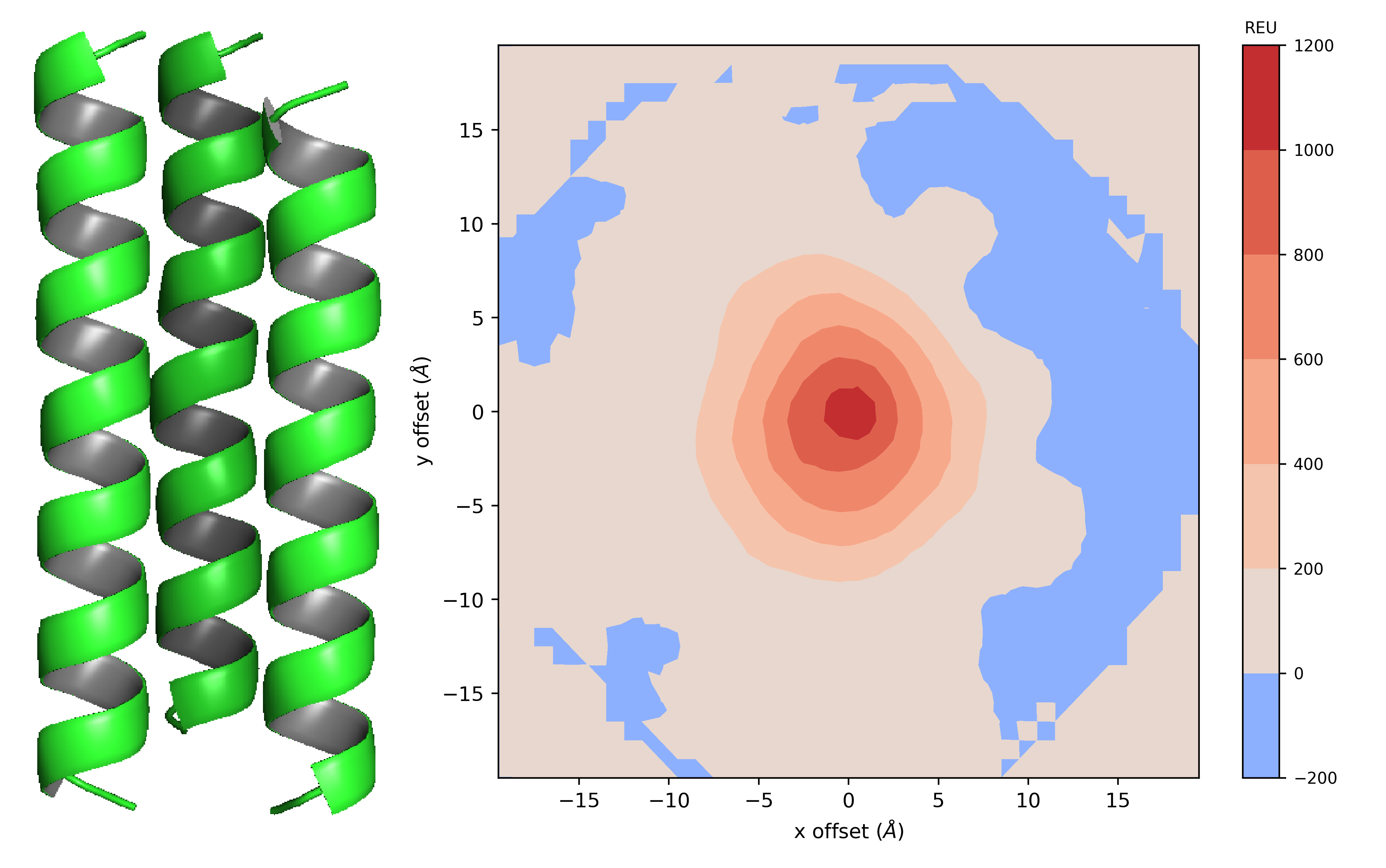
Figure 1: We tested our algorithm against a known three helix bundle (PDB ID: 4TQL, left panel). Loops were excised and helices were shortened to allow their free movement for our proof-of-concept study. The right panel shows the energy landscape of a pair of $\alpha$-helices selected from the bundle in two dimensions while fixing their internal conformations, rotational orientations, and z-offset (along the axis of the helices) to zero with respect to the native structure. For relative displacements less than the diameter of a single $\alpha$-helix ($\sim 6$ $\AA$) the interaction energy rapidly grows large, while for relative displacements greater than $\sim 15$ $\AA$, the interaction energy goes to zero. In between, when the helices are in close proximity without backbone clashes, sidechain-sidechain steric repulsion often results in high energies. At slightly greater separation, there appear negative energy wells (blue) indicating mutual attraction. Note that though we are showing a two-dimensional energy landscape here, three helix rigid body docking in two-dimensional translation space requires us to sample configurations from a six-dimensional phase space.

Next, we considered the size of simulation space which, given the two mobile bodies of our problem, can fit onto the Pegasus graph topology of the D-Wave Advantage 4.1 quantum annealer, the largest available quantum annealer at the time of experiment. Considering that with a one-hot encoding our approach requires a fully-connected QUBO graph, the connectivity and size of the available hardware limits embeddings to graphs containing up to 177 binary variables, admitting a largest chain length of 17 qubits d_wave_white_paper_advantage . A cubic simulation space with $N=3$ bodies would therefore be limited to $T=4\times 4\times 4$ points with the current hardware, the number of variables required being $(N-1)T$. To allow more points per dimension, we opted instead to simulate over a square planar space, perpendicular to the known axis of the bundle. With $N=3$ bodies, a maximum of $T=8\times 8$ points may be simulated for such a space with the current hardware. To guarantee embedding of the problem graph and reduce the required chain length, we selected a slightly smaller space of $T=7\times 7$. Physically, the separation of adjacent points within this space corresponds to a distance of 3 $\AA$, so that its physical dimensions are $18\times 18$ $\AA$. This selection accommodates both the possibility of separation between the helices and their close proximity, given that the step size of 3 $\AA$ is smaller than the $\sim 6$ $\AA$ diameter of an $\alpha$-helix.

Using Rosetta, we then pre-computed the possible pairwise energies between each pair of rigid-body helices within each simulation space using REF2015_soft, these energies forming the basis of the energy landscape for both the quantum annealing approach and simulated annealing approaches. For a given pair of $\alpha$-helices, their pairwise energy landscape is strongly positive when their separation distance is overlapping, goes to zero when their separation distance is far, and in between exhibits dips where mutual attraction occurs (see Figure 1). Since this small example problem allows only $49^{2}=2,401$ possible physical solutions, we exhaustively enumerated the energies of each of these solutions to provide a ground truth to compare to, specifically considering those physical states exhibiting negative energy. We shall refer to the full set of these states, constituting our target diversity, as $S$.

Note that with a problem size of $N=3$ and the grid size tested, the number of pairwise pre-computations is greater than the number of possible physical solutions. However, for $N>3$, the number of pairwise pre-computations grows only quadratically while the number of physical solutions grows exponentially with $N$. This means that the number of pairwise pre-computations becomes exponentially less in $N$ than the number of possible physical solutions.

II.5 Quantum annealing

After pre-computing the $h(b_{i}^{x})$ and $J(b_{i}^{x},b_{j}^{y})$ energies for the three helix bundle problem, we capped highly-positive pairwise energy values at approximately twice the magnitude of the largest negative pairwise energy value. This reduces the variance of spin couplings and biases upon embedding the problem on the D-Wave QPU, which has limited dynamic ranges to its biases and couplers, thereby increasing the energy separation between lower-energy states upon embedding. The importance of this step is in reducing the impact of integrated control errors, which affect solution quality increasingly as separation between low-energy states decreases d_wave_ice . Originally, the largest positive pairwise energy in the QUBO registered above $5000$, but with energy-capping based on the largest negative pairwise energy of $-38$, large positive energies reduced to $100$.

In keeping with the findings of Zucca et al., where a search over anneal time was performed and evaluated with respect to maximizing solution diversity over three classes of Ising problem zucca2021diversity , we selected to work with an anneal time of 1 $\mu$s. We then conducted a preliminary search over the strength of the one-hot penalty constant $\gamma$ between $10^{0}$ and $10^{3}$, executing 25 replicates of $10^{4}$ successive samples each, recording the best energy and proportion of target solution diversity found per replicate. Further, we downsampled each replicate using a sliding window between $10^{2}$ and $10^{4}$ samples to investigate trends in best energy and solution diversity as functions of sample size. (Note that a metric computed using a smaller sample size gets averaged over a larger number of replicates.) For each solution returned by the D-Wave solver, we also applied a classical steepest-descent bit-flip optimizer (greedy post-processing) to find the local minimum in each solution neighborhood before recording solution diversity and quality as functions of one-hot penalty strength and number of samples as before. This optimizer has a run-time complexity of $\mathcal{O}(NT)$ per step, with experiments showing an average of 5 steps required per solution returned by the quantum annealer, irrespective of $\gamma$.

Next, we computed from these data the success probability of finding the target diversity and ground state energy as a function of number of samples by downsampling, per each tested value of gamma. Specifically, we compute success probability by counting the number of replicates exhibiting target diversity or containing the ground state and dividing by the total number of replicates for a given value of one-hot penalty strength and given number of samples. For each one-hot penalty strength, we then fitted sigmoid curves of the form:

$$y=\frac{1}{1+e^{\alpha(t-t_{0})}},$$ (4)

to the corresponding success probability functions, and took the resulting, fitted $t_{0}$ parameters as the number of samples required to reach target diversity or best energy with 50% confidence.

II.6 Simulated annealing

To understand better the performance and behaviour of the D-Wave quantum annealer, we also tested a classical QUBO simulated annealing solver. This approach works over exactly the same energy landscape as the quantum annealer, and also includes both physical and non-physical states whose separation is tunable by the strength of the one-hot penalty. We specifically employ the D-Wave simulated annealing sampler, which accepts QUBO problems and updates bits according to the Metropolis-Hastings criterion. Using default parameters, we repeated the same experiments and analysis as for the quantum annealer.

III Results and Discussion

We organize our results and discussion as follows. In section III.1, we provide a demonstration of a multibody docking problem solved in all-atom detail, using a robust Rosetta REF2015_soft energy function, on the quantum annealer. This serves as a proof of principle that multibody docking problems can be mapped to quantum hardware, and that a quantum annealer can produce meaningful results. In section III.2, we discuss general effects of tuning the one-hot QUBO penalty strength on the intermixing between physical and non-physical states, and on the ruggedness of the energy landscape. Further, we point to a means of estimating the degree of this mixing and ruggedness in advance of sampling. In section III.3, we present and discuss the specific dependence of solution diversity of the three helix bundle problem on the one-hot penalty strength, as sampled by D-Wave Advantage 4.1 and the QUBO simulated annealing solver, including time-to-target diversity results. In section III.4, we present and discuss the specific dependence of solution quality of our problem on one-hot penalty strength, including time-to-target solution results.

III.1 Multibody docking on a quantum annealer proof of principle

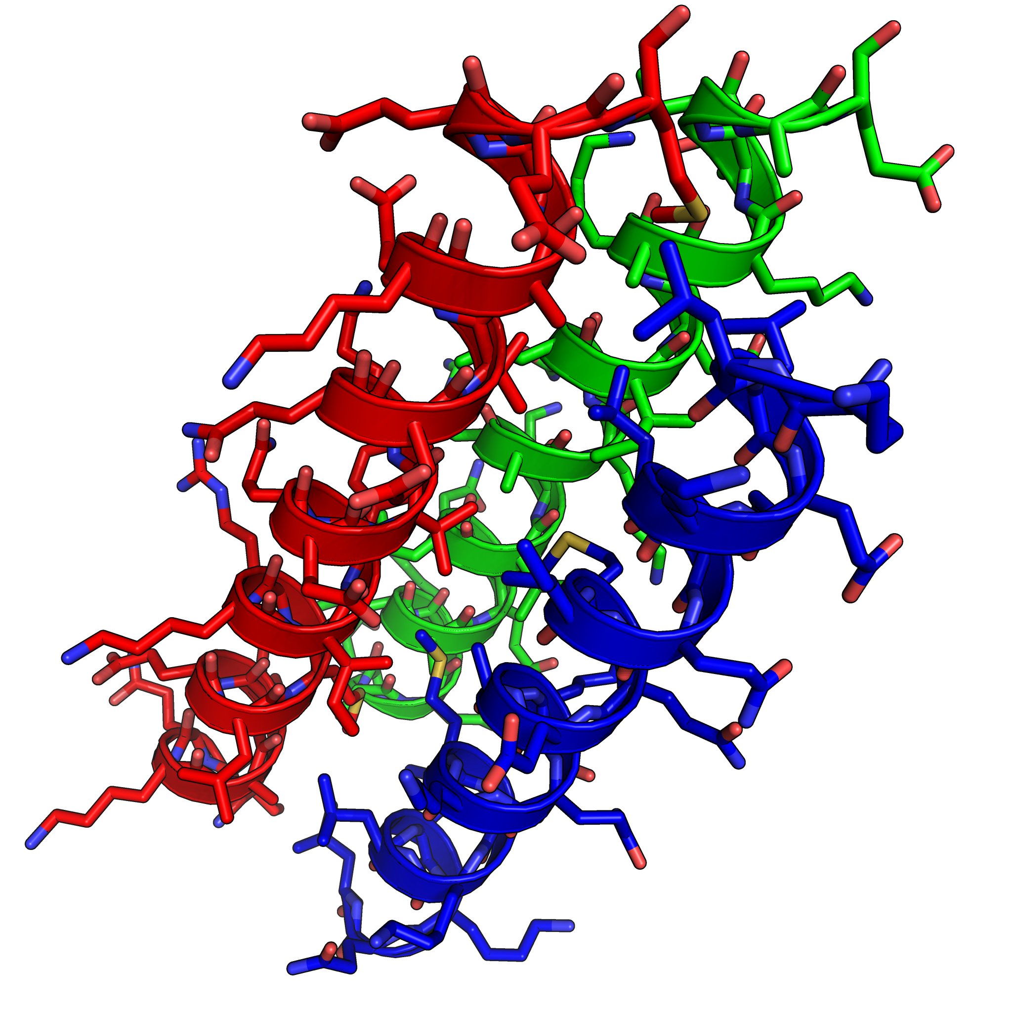
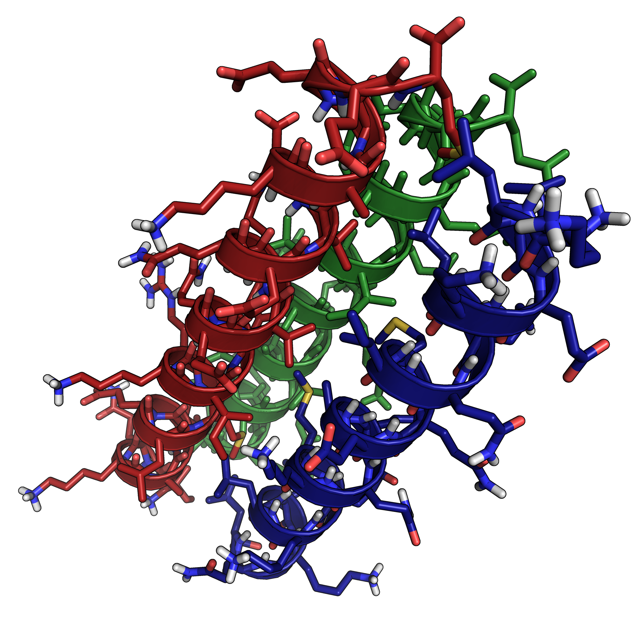
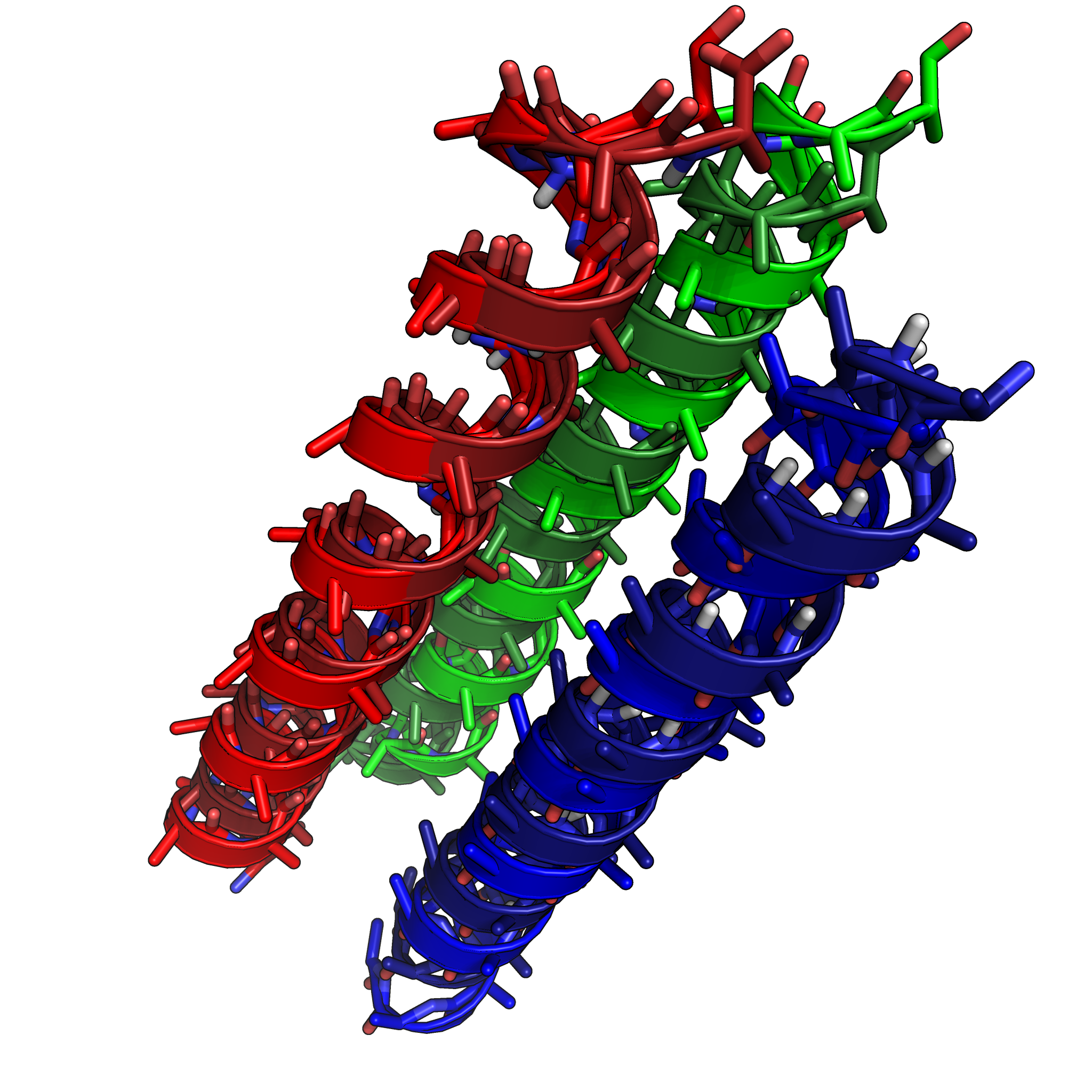
Figure 2: Comparison of actual structure (left panel) and predicted lowest-energy structure from the quantum annealer (middle panel, with main-chain overlay in right panel). The three helices are shown in red, blue, and green respectively, with darker colours for the prediction. The mainchain heavyatom RMSD between prediction and actual structure was 2.4 $\AA$, which is less than the 3.0 $\AA$ spacing of the sampled grid.

As described in section II.4, we constructed a simple three-body docking problem ($N=3$) to test our method by dividing an $\alpha$-helical protein into three helical fragments. In order to fit the problem to the currently-available quantum annealing hardware, we fixed one of the helices and sampled 49 points ($T=49$) in the two-dimensional physical space for each of the other two helices. The space sampled was a plane perpendicular to the bundle axis. Given a fixed helix, the sampling problem at hand corresponds to finding the lowest energy configuration in a twelve-dimensional solution space, reduced to four dimensions by considering only translations in the plane of the other two helices.

Of the $T^{N-1}=2,401$ possible solutions to this small three-body docking problem, exhaustive enumeration revealed that the lowest-energy solution had an RMSD of 2.4 $\AA$ from the native structure of the protein as determined by x-ray crystallography; that is, given that the translational grid spacing was 3.0 $\AA$, the global minimum for this problem given the energy function used does indeed correspond to the true minimum to the limits of sampling resolution. We found that with greedy post-processing, the D-Wave quantum annealer was able to find this solution reliably with fewer than 100 samples when hyperparameters were optimally tuned (see section III.4 for full details), providing a simple proof of principle that problems of this class can be solved by quantum annealing. Note that although this problem was simplified by using sparse grid sampling on a subspace of the full twelve-dimensional solution space, no simplification was made to the representation of the molecule: energies were computed for the all-atom models of the helices, using the full Rosetta REF2015_soft energy function. Figure 2 shows the x-ray crystal structure of the portion of the protein modelled compared to the predicted docked configuration of the three $\alpha$-helices.

III.2 Penalty strength influence on intermixing of physical and non-physical states

We consider Equation 3 in three different regimes of the one-hot penalty strength, $\gamma$: (1) the large $\gamma$ regime: when $\gamma$ is large enough that physical and non-physical states are separate, (2) the moderate $\gamma$ regime: when $\gamma$ is such that there is mixing between physical and non-physical states, but some physical states are lower in energy than all non-physical states, and (3) the small $\gamma$ regime: when $\gamma$ is such that there is mixing between physical and non-physical states, but some non-physical states are lower in energy than all physical states. In Figure 3, the frequencies with which the D-Wave quantum annealer samples states as functions of state energy are shown for each of these cases.

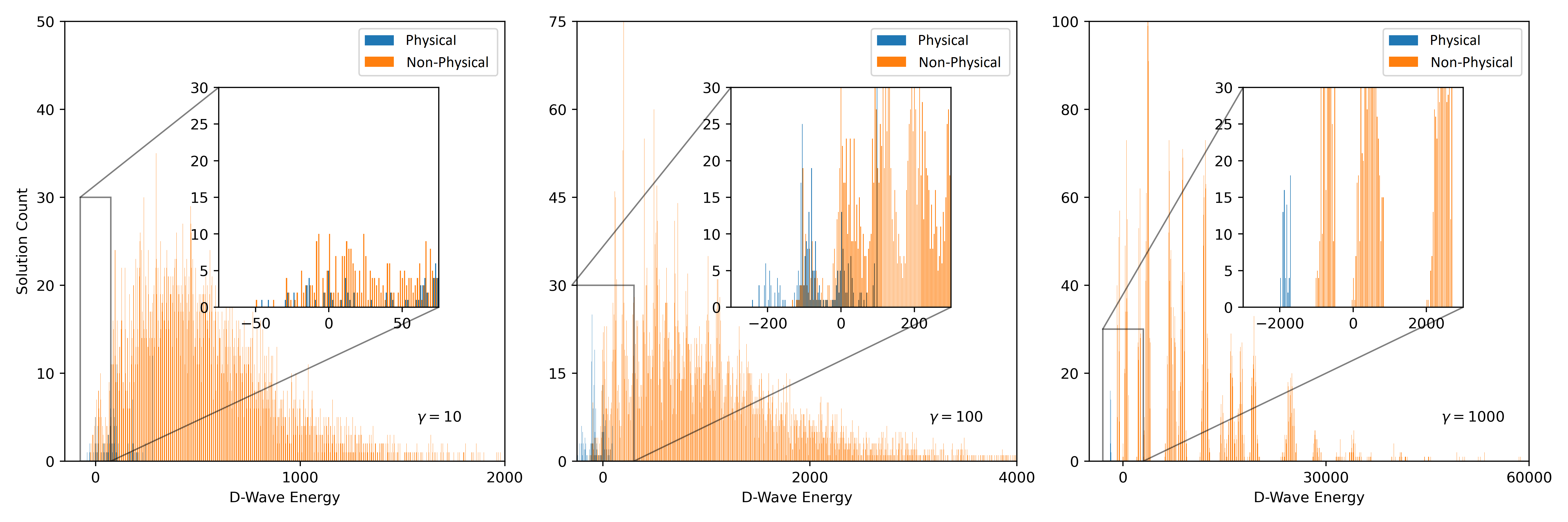
Figure 3: Sample solution energy distributions returned by D-Wave Advantage 4.1 of one-hot three helix bundle docking problem QUBO sampled $10^{4}$ times with annealing time $\tau=1$ $\mu$s, for one-hot penalty strength $\gamma=10$ (left panel), $\gamma=100$ (central panel), and $\gamma=1000$ (right panel). Physical and non-physical solutions are shown in blue and orange, respectively. When $\gamma=10$ (small $\gamma$ regime), total mixing between physical and non-physical states occurs, so that the lowest and highest energy states are non-physical. When $\gamma=100$ (moderate $\gamma$ regime), some mixing between physical and non-physical states occurs; note, however, that the lowest energy states are physical. When $\gamma=1000$ (large $\gamma$ regime), physical and non-physical states are separated. In all cases, non-physical states are sampled with higher frequency than physical states, though sampling of low-energy physical states is most efficient in the moderate $\gamma$ regime.

In the large $\gamma$ regime, at the extreme where $\gamma\gg|E|$, with $|E|$ being the largest-magnitude energy term appearing in Equation 3, we get the following QUBO:

$$H_{\text{MBD}}(\gamma\gg|E|)\approx\gamma\sum_{x\in X^{\prime}}\Big{(}-\sum_{i=1}^{T}b_{i}^{x}+2\sum_{i>j}b_{i}^{x}b_{j}^{x}\Big{)}.$$ (5)

In this regime, all $T^{N-1}$ physical states have an approximate energy of $-\gamma(N-1)$, while all non-physical states correspond to higher energies, the lowest non-physical excited state having an approximate energy of $-\gamma(N-2)$ (see Appendix A for details). All local minima correspond to physical states, so that one can always move downhill by successive bit-flips from any non-physical state to a physical state in this regime. However, once in a physical state, it’s impossible to move further downhill by local bit-flips. (Note that moving in this way, one has no guarantee of finding a physical state of interest, such as one of energy below a desired threshold.) As we reduce the value of $\gamma$, we enter the moderate $\gamma$ regime by uplifting the quasi-degeneracy of physical ground states, along with reducing the gap between physical states and the first excited non-physical state.

In the moderate $\gamma$ regime, only those physical states with energies lower than all non-physical states are guaranteed to be local minima. This has the effect of reducing the number of local minima in the landscape. Due to the intermixing between physical and non-physical states, it is sometimes possible to move downhill from a physical state using local bit-flips by first moving to a non-physical state and then to a lower-energy physical state. While this does not guarantee that low-energy physical states will be found, it increases the paths by which one could be found, and thereby increases the likelihood that these states will be found.

Upon entering the small $\gamma$ regime, certain non-physical states start to appear as local minima as they take on energies less than the energy of any physical state. Starting from either a physical state or a non-physical state higher in energy, it is often possible to move downhill by local bit-flips. However, one often gets stuck in a non-physical local minimum. Continuing to decrease $\gamma$, a threshold is reached whereupon all local minima are non-physical states.

Appendix A describes in detail how to efficiently estimate the bounds of physical and non-physical state distributions as a function of $\gamma$ given only the energy scale and number of quantum registers of a one-hot QUBO. This allows one to estimate in advance the value of $\gamma$ required to separate fully between physical and non-physical states, for example, or the value required to expose a certain percentage of the physical state energy band, a useful first step in tuning the ruggedness of the energy landscape to suit the needs of a particular problem.

III.3 Solution diversity

In Figure 4, we present the diversity of low-energy physical states sampled by the D-Wave quantum annealer and QUBO simulated annealing sampler over the three regimes of one-hot penalty strength $\gamma$, which was discussed before. These regimes correspond to various degrees of mixing between physical and non-physical states.

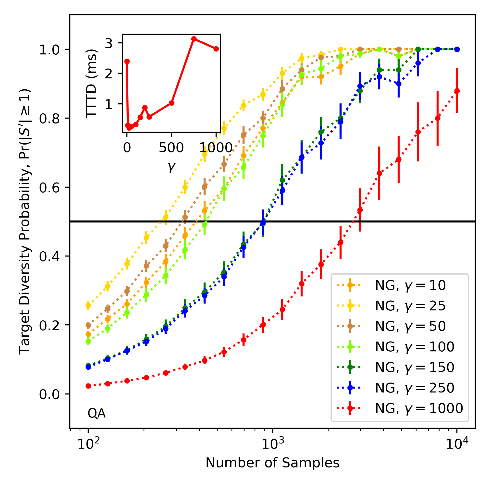
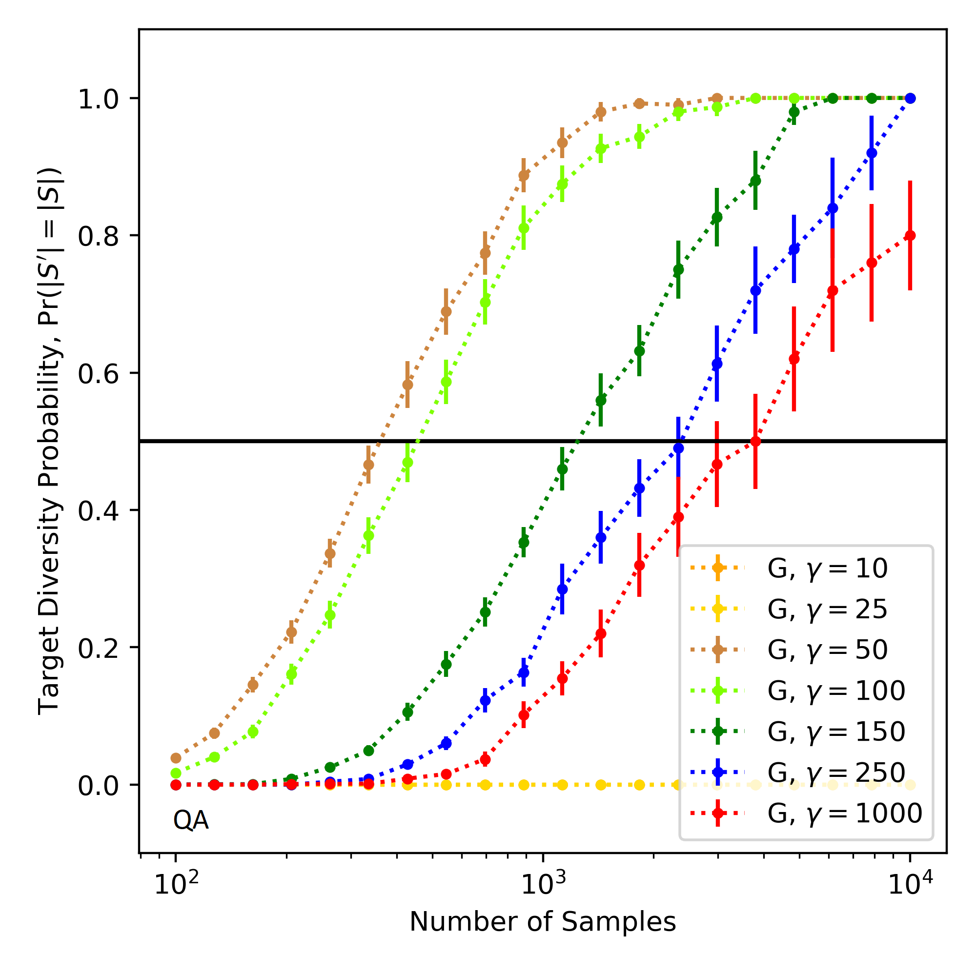
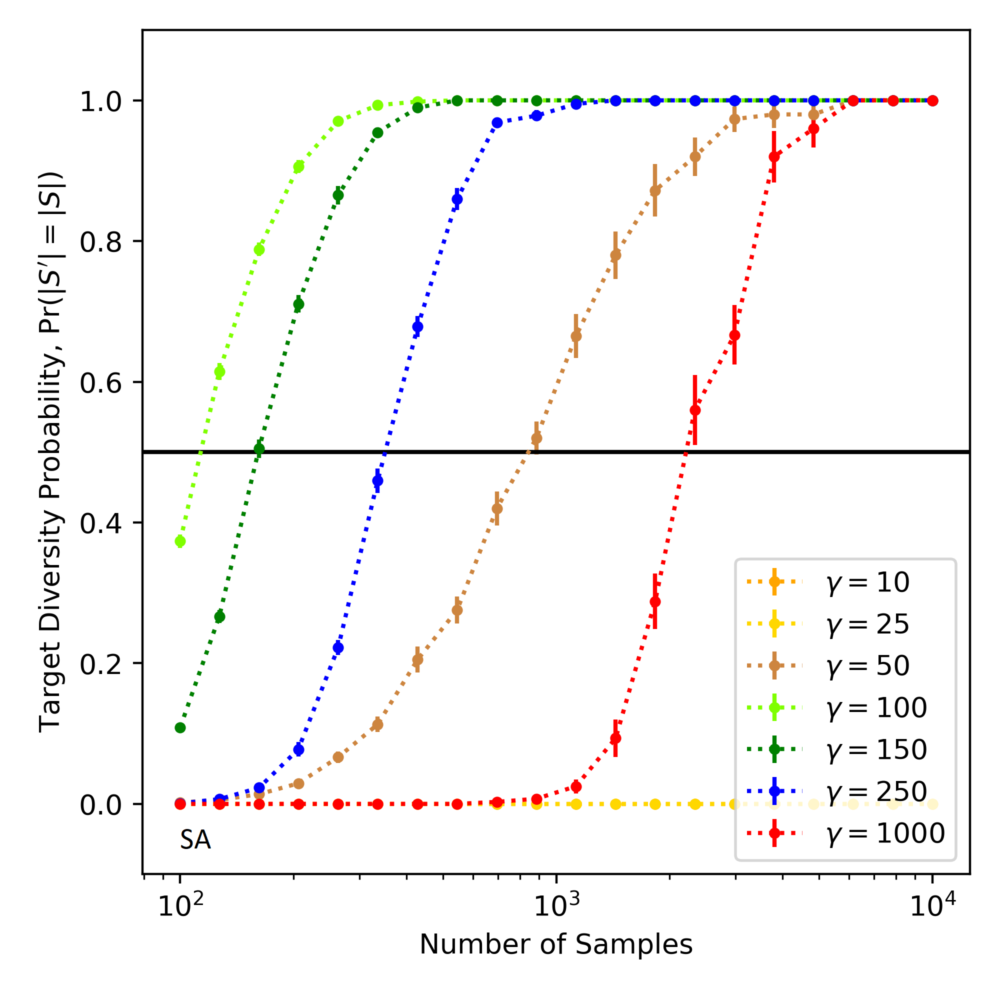
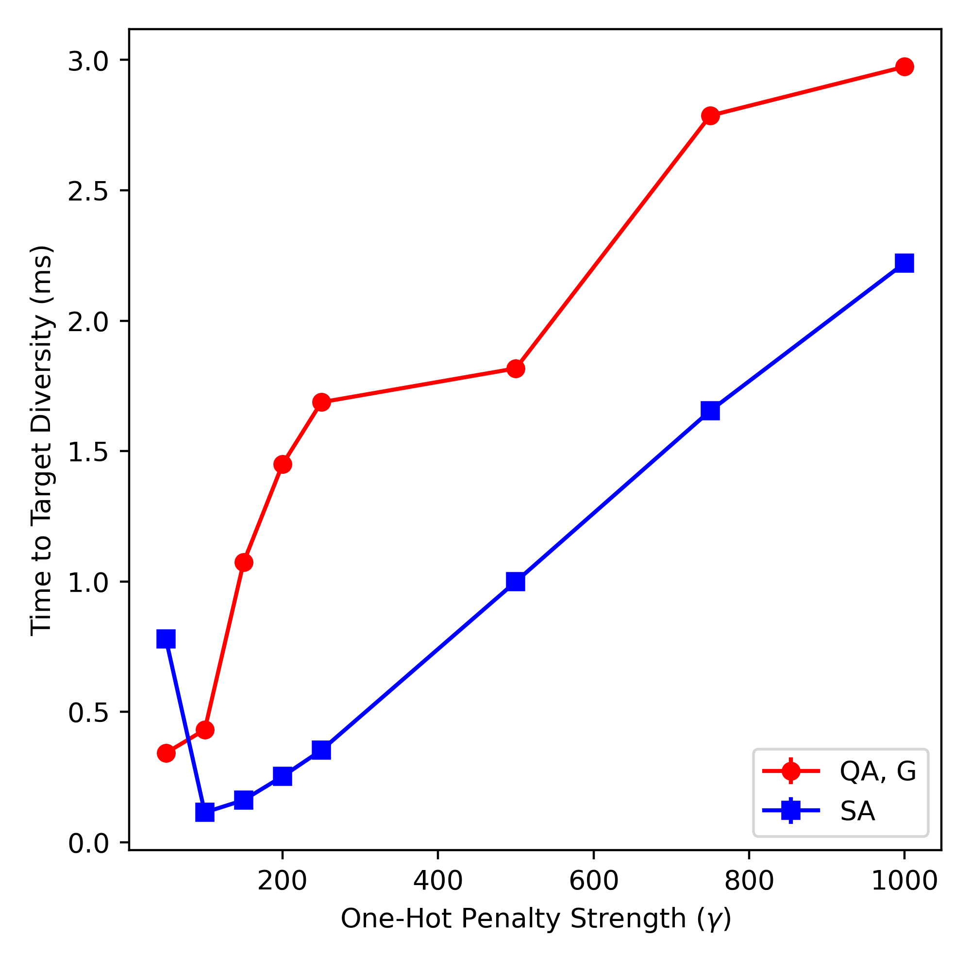
Figure 4: (Upper left) Three helix bundle target diversity probability shown as a function of sample size without greedy post-processing (NG for non-greedy). On the y-axis, we have $\text{Pr}(|S^{\prime}|\geq 1)$, which is the probability of the D-Wave quantum annealer sampling a subset $S^{\prime}\subset S$ of at least one target state from the set of target states in the given number of samples. Inset: Time-to-target diversity (TTTD), based on 50% probability of achieving target diversity, plotted as a function of $\gamma$. TTTD is minimum for $\gamma=25$. (Upper right and lower left) Target diversity probability as a function of sample size for (upper right) quantum annealing with greedy post processing and (lower left) QUBO simulated annealing. On the y-axis, we have $\text{Pr}(|S^{\prime}|=|S|)$, which is the probability of the quantum annealer sampling the full target diversity. Full target diversity is achieved with fewest samples for the two algorithms (greedy post-processing and QUBO simulated annealing) at $\gamma=50$ and $\gamma=100$, respectively. (Lower right) Quantum annealing with greedy post-processing and simulated annealing time-to-target diversity as a function of $\gamma$. Note that only the annealing time of 1 $\mu$s is counted toward TTTD in the case of quantum annealing. A single simulated annealing sample is estimated as 1 $\mu$s assuming each step of the 1000 steps constituting the anneal schedule to take 1 ns.

Focusing first on the solutions returned by the D-Wave quantum annealer prior to greedy post-processing (non-greedy), we investigate target diversity through the probability of the sampler returning at least one state from the target set within a given number of samples. We see that in starting from small $\gamma$ ($<10$), as we increase $\gamma$ slightly to $10\leq\gamma\leq 50$, we decrease the number of samples required to achieve full diversity. Increasing $\gamma$ beyond $50$ to $100$ serves to worsen the time required to achieve full diversity. We see a similar trend in average normalized diversity, i.e. the average number of negative energy states divided by the number of target states (Figure A.2, left panel, and inset Figure A.3, left panel).

Upon greedy post-processing, some to all target states are brought to either other lower-energy target states, or to non-physical states, for those values of $\gamma$ tested less than 50 (1, 10, 25). As a result, we see that the full diversity is unachievable for these values of $\gamma$. Figure A.3 (left panel) best demonstrates this effect, showing that for $\gamma\leq 10$ in particular, no target states are found with greedy post-processing, while for $\gamma\geq 50$, all target states are found in the large sample limit. This indicates that $\gamma\leq 10$ lies in the small $\gamma$ regime, while $\gamma\geq 25$ lies in the moderate $\gamma$ regime, where $\gamma\geq 50$ is required to fully expose the physical states corresponding to the target set $S$. We see that at this value of $\gamma=50$, $S$ is fully sampled more rapidly compared to greater values of $\gamma$ as seen from the trend of normalized diversity as a function of $n$ samples (Figure A.3, left panel).

Interestingly, we note that between non-greedy and greedy post-processing of the quantum annealer solutions, different values of $\gamma$ demonstrate best performance as judged by the minimal number of samples required to achieve the target diversity with $50\%$ confidence. In the non-greedy case, $\gamma=10$ demonstrates fastest convergence to the target set of states (Figure 4, upper-left panel), while in the greedy case, $\gamma=50$ performs best (Figure 4, upper-right panel). The latter we suggest should be true due to the following: when $\gamma=50$, as discussed, the physical part of the spectrum of states corresponding to the target set becomes fully exposed, so that the energy landscape then essentially consists in 13 local minima, each corresponding to a target state. All other sampled states, which are preferentially non-physical states (see Figure 3), are brought by greedy descent with overwhelming likelihood to one of the 13 target states by an average of 5 iterations of the greedy descent optimizer. As $\gamma$ increases, more local minima are exposed, so that a given bit-string will be optimized by greedy descent with less likelihood to one of the target states. For $\gamma<50$, there are fewer physical minima than the target states, which makes it impossible to reach the full target set.

For QUBO simulated annealing, as with greedy quantum annealing, all samples for $\gamma\leq 25$ represent non-physical states, or otherwise a subset $S^{\prime}\subset S$, so that full target diversity is never achieved within this regime. QUBO simulated annealing fully samples $S$ at $\gamma=50$; however, the required minimal number of samples to achieve full target diversity is higher than in the range of $100\leq\gamma\leq 250$ (Figure 4, lower-left panel) . In contrast, greedy quantum annealing produces the shortest time (minimal number of samples) to sample S at $\gamma=50$. We suspect that the difference between the two methods arises because when $\gamma=50$, simulated annealing converges to the exact ground state more frequently when compared to D-Wave sampling due to hardware noise on the latter. To sample better the target diversity with simulated annealing, one needs to increase the height of the barriers between local minima by increasing $\gamma$, so that with a higher probability the simulated annealer gets stuck in the higher-energy states that constitute the target diversity. However, increasing $\gamma$ beyond the range of $100\leq\gamma\leq 250$ decreases the probability of achieving the target set, since the probability of the simulated annealer being stuck in non-target minima increases.

In comparing greedy quantum annealing and QUBO simulated annealing time-to-target diversity (Figure 4, bottom-right panel), under the clock-time assumptions made for each, QUBO simulated annealing appears to outperform greedy quantum annealing by a constant factor of approximately 1.5 over most values of $\gamma$ tested, for the three helix bundle problem. However, at this stage, no definitive conclusions might be drawn concerning the general performance of these two methods, or their scaling. The latter requires that they be assessed relative to a continuum of problem scales, which within the context of molecular docking entails varying the number of docking bodies ($N$). It should be noted as well that, although $\gamma=400$ approximates the common recommendation that one should choose a one-hot penalty strength about four times the maximum energy of the problem QUBO, we see an approximately 4-fold time savings in the case of greedy quantum annealing, and a 4-fold time savings in QUBO simulated annealing in comparing time-to-target diversity between optimized $\gamma$ and $\gamma=400$.

These investigations suggest a different “sweet spot” for $\gamma$ under each method of sampling with respect to the desired target diversity, all of which, nevertheless, require intermixing between physical and non-physical states. In the case of greedy quantum annealing and QUBO simulated annealing, due to the steepest-descent step that forms the end stage to each (effected through the low-temperature stage in simulated annealing), it is the ruggedness of the landscape and how widely this landscape is sampled that combine to determine the number and distribution of local minima achieved. In general, larger $\gamma$ equates to more physical local minima and larger energy barriers between them. In the case of non-greedy quantum annealing, non-minima are sampled in addition to local minima due to hardware noise, so that the optimal choice of $\gamma$ is more a reflection of which energy band is preferentially sampled by the D-Wave solver. In our example, this energy band required full mixing between physical and non-physical states. It remains to be studied over a range of problems how to specifically select an optimal value of $\gamma$ for a given solver, but this work suggests that for each case energy mixing is required.

III.4 Solution quality

In Figure 5, we present the relative performance of the D-Wave quantum annealer and QUBO simulated annealing sampler as measured by their ability to sample the ground state for our problem over a range of one-hot penalty strengths. As observed for solution diversity, non-greedy quantum annealing (Figure 5), upper-left panel) demonstrates best performance with respect to the known ground state when $\gamma=10$, which occupies the small $\gamma$ regime of strong intermixing between physical and non-physical states. Increasing $\gamma$ reduces the probability of achieving the ground state in monotonic fashion until $\gamma=1000$, where the ground state solution is never sampled. We expect that for $\gamma>1000$ we should continue to see failure to sample from the ground state due to limited dynamic range causing increased quasi-degeneracy of physical states and an increase in the effect of hardware noise. Note that over all $\gamma$, unit probability of sampling the ground state over the sample range tested is not achieved; at best, when $\gamma=10$, a probability of 0.23 of sampling the ground state over $10^{4}$ samples is achieved.

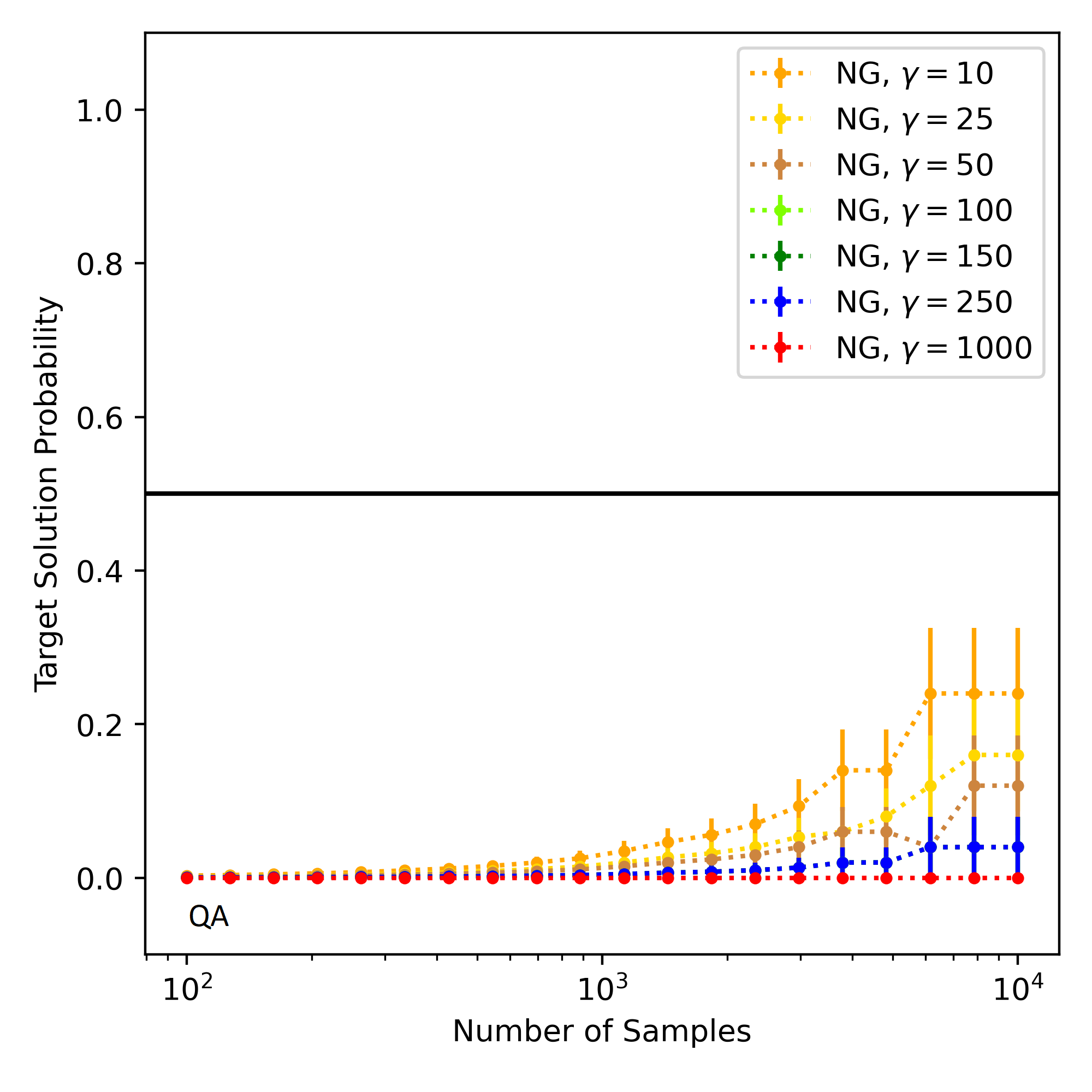
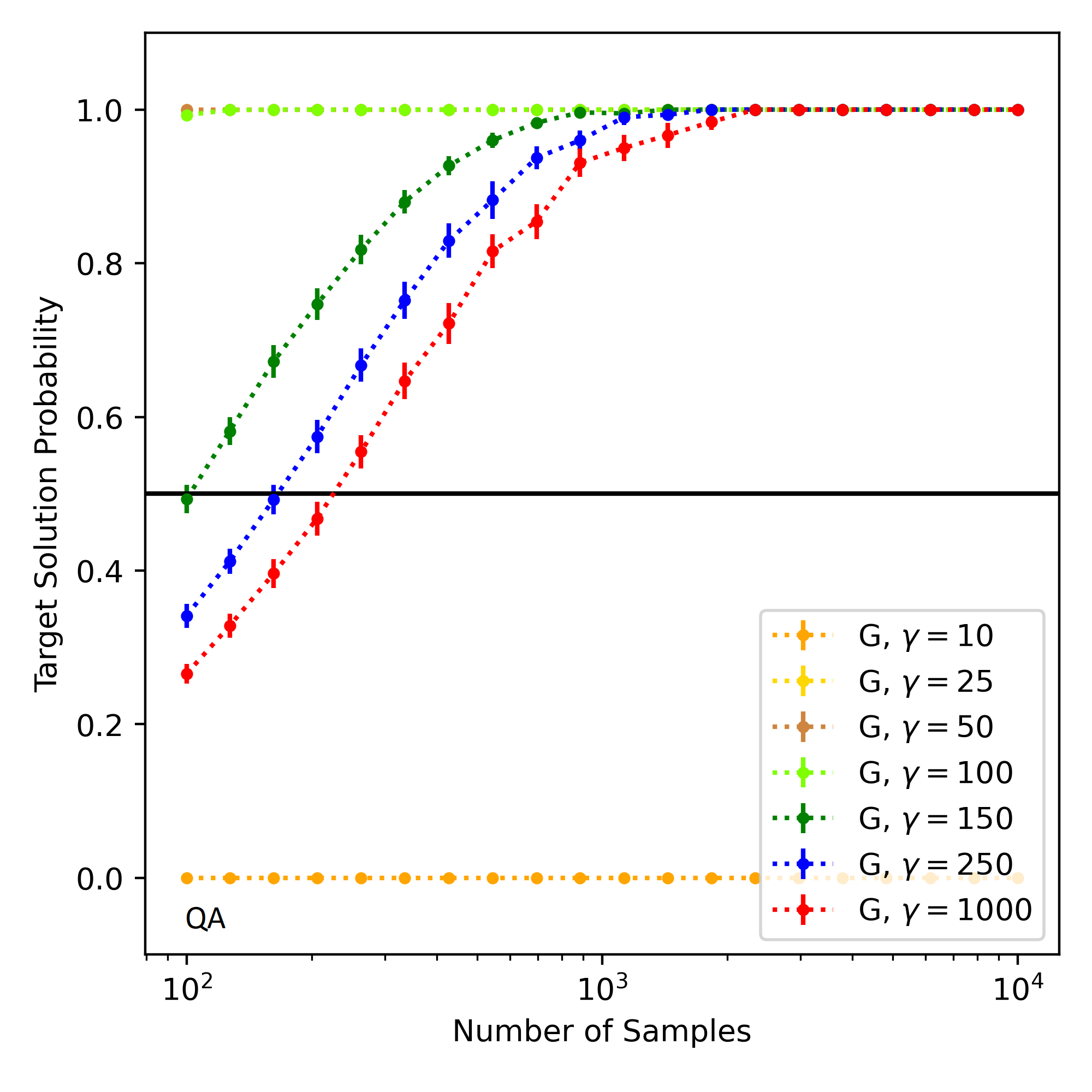
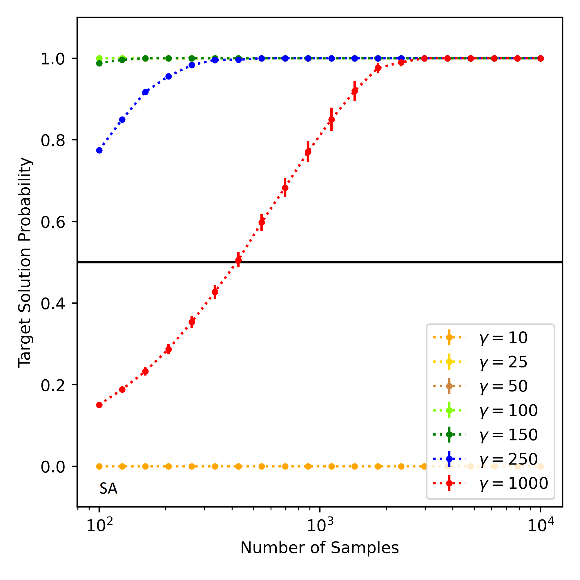
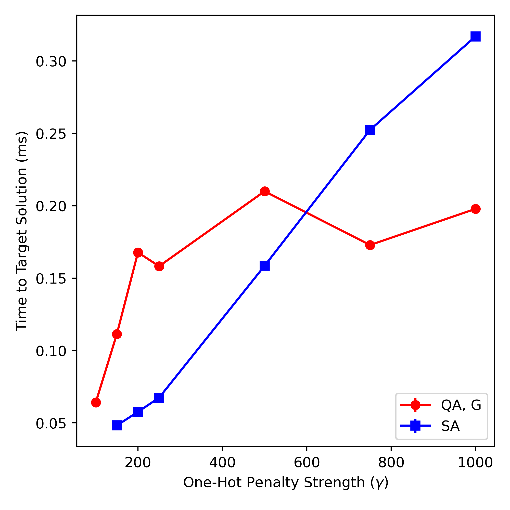
Figure 5: Three helix bundle ground state target solution probability as a function of number of samples for: (upper left) quantum annealing without greedy post-processing (NG for non-greedy), (upper right) quantum annealing with greedy post-processing, and (lower left) QUBO simulated annealing. Panels contain solver labels in their lower-left corners. (Lower right) Quantum annealing with greedy post-processing and QUBO simulated annealing time to target solution as a function of $\gamma$. Note that only the annealing time of 1 $\mu$s is counted toward TTTD in the case of quantum annealing. A single simulated annealing sample is estimated as 1 $\mu$s assuming each step of the 1000 steps constituting the anneal schedule to take 1 ns.

In the case of quantum annealing with greedy post-processing (Figure 5, upper-right panel), for $\gamma>10$, the ground state solution is reached with unit probability in the large sample limit, with smaller values of $\gamma$ demonstrating faster convergence. Note that while best performance over the set of 13 diverse target solutions required $\gamma=50$, here, the smaller value of $\gamma=25$ is optimal. This corresponds to less exposure of the physical spectrum. In other words, a smaller number of local physical minima are present, which increases the probability that a steepest descent optimizer should bring a sampled bit-string to the ground state. Indeed, for $\gamma\leq 100$, near-unit probability of sampling from the ground state is achieved in only 100 samples. For $\gamma>100$, a substantially greater number of samples is required to guarantee unit probability of sampling the ground state. As discussed in section III.3, this dependence on $\gamma$ is a result of the number of local minima increasing with $\gamma$, so that a sampled bit-string is less likely to converge to the ground state with greedy descent. It is expected that as problems grow larger any more complex, with larger $T$ (number of gridpoints per body) and $N$ (number of bodies), the probability of a random bitstring converging to the global optimum with greedy descent would drop considerably at any value of $\gamma$, so that while the tuning of $\gamma$ is important, greedy descent alone cannot be relied upon.

The probability of finding the optimal solution as a function of sample size with QUBO simulated annealing is shown in the lower-left panel of Figure 5. The performance of QUBO simulated annealing displays precisely the same monotonic dependence on $\gamma$ as does greedy quantum annealing, though faster convergence in terms of number of samples required is observed for all $\gamma<750$ (Figure 5, bottom-right panel). For $\gamma\geq 750$, the greater number of samples required for QUBO simulated annealing suggests that quantum annealing samples preferentially from the low-energy well containing the ground state as its minimum in the large $\gamma$ regime versus QUBO simulated annealing. We remark that this plateauing for greedy quantum annealing constitutes an interesting departure from the roughly linear scaling in $\gamma$ seen for: (i) QUBO simulated annealing on the time-to-solution metric, and (ii) greedy quantum annealing and QUBO simulated annealing on the time-to-target diversity metric.

Again, as in the case of solution diversity, we observe that the one-hot formulation of our multibody molecular docking problem shows better performance when the one-hot penalty strength, $\gamma$, is tuned to promote mixing between physical and non-physical states. Specifically, we see a 3-fold time savings in the case of greedy quantum annealing, and a 3-fold time savings in QUBO simulated annealing in comparing between optimized $\gamma$ and $\gamma=400$, a selection approximating the recommended practice that chooses a one-hot penalty strength about four times the maximum energy of the problem QUBO. Optimized $\gamma$, as with solution diversity, varies with solver. In the case of non-greedy quantum annealing, we observe that the same choice of $\gamma$ optimizes against both solution diversity and quality for the three helix bundle problem, while different $\gamma$ are optimal for greedy quantum annealing and QUBO simulated annealing. It is likely that varying the target diversity may require different $\gamma$ for non-greedy quantum annealing solution diversity and quality.

IV Conclusion

In this work, we have shown that the multibody molecular docking problem, critical to the computational drug discovery pipeline, can be mapped to a form executable by current- and future-generation quantum annealing hardware using a one-hot encoding scheme. This mapping involves a classical pre-computation of pairwise interactions followed by sampling executed on a quantum annealer. Since the classical pre-computation scales only quadratically in the number of docking bodies, our approach delegates the harder part, sampling low-energy states in an exponentially large solution space, to the quantum annealer. Our approach is notable for being able to leverage any pairwise-decomposable energy function, including the highly optimized Rosetta REF2015 energy function, without loss of fidelity.

Testing our method against a realistic three-body problem, we observe that quantum annealing is able to sample diverse low-energy configurations reliably, especially when coupled with greedy-descent post-processing. These configurations include the ground state matching the experimentally-determined configuration to within the spacing of our sampling grid. Importantly, we observe that one-hot penalty strengths that allow intermixing of physical and non-physical states can increase the probability of sampling from these configurations by approximately 3-4 times when compared to recommended penalty strengths that do not allow intermixing. We find that this is because one-hot penalty strength effectively tunes the intermixing of physical and non-physical states, which in turn tunes the number of local minima. As assessed by the three body problem tested, we observe comparable performance between quantum annealing and QUBO simulated annealing.

In this work, we have replaced the $NP$-hard step of the multibody docking problem with quantum sampling that can conceivably show better-than-classical performance scaling as quantum hardware grows larger and more robust. Since we have done this without sacrificing accuracy in the polynomial-time energy pre-computation, we hypothesize that our approach could offer performance advantages for large multibody docking problems over classical approaches in the future. Because multibody docking is a rate-limiting step when validating designed drugs binding to their targets in silico, particularly when bound water molecules are modelled explicitly, this work has the potential to greatly accelerate drug discovery pipelines.

Appendix A Estimating the inter-mixing effects of one-hot penalty strength

The general one-hot multibody docking Hamiltonian for a set $X=\{1,2,...,N\}$ of bodies is:

$$H =\sum_{x\in X}\sum_{i=1}^{\alpha_{x}}\big{(}O(b_{i}^{x})-\gamma\big{)}b_{i}^{x}$$

$$+\sum_{x\geq y}\sum_{i>j}(T(b_{i}^{x},b_{j}^{y})+\delta)b_{i}^{x}b_{j}^{y}$$ (A.1)

This Hamiltonian admits internal, rotation, and translational degrees of freedom, where $\alpha_{x}$ is the number of binary variables representing the possible body-configurations of body $x\in X$.

Ignoring internal and rotational degrees of freedom, this Hamiltonian simplifies to:

$$H =\sum_{x\in X^{\prime}}\sum_{i=1}^{\alpha}\big{(}O(b_{i}^{x})-\gamma\big{)}b_{i}^{x}$$

$$+\sum_{x\geq y}\sum_{i>j}(T(b_{i}^{x},b_{j}^{y})+\delta)b_{i}^{x}b_{j}^{y}$$ (A.2)

$X^{\prime}=\{1,2,...,N-1\}$ is the set of mobile bodies (where we have selected body $N$ from $X$ to be fixed), and $\alpha$ is the number of translational grid-points accessible to any of these mobile bodies. The $O(b_{i}^{x})$ terms then represent the pairwise energies of mobile body $x$ relative to the fixed body, and the two body terms $T(b_{i}^{x},b_{j}^{y})$ the pairwise energies between mobile bodies $x$ and $y$. Recall that $\delta=2\gamma$ if $x=y$ and is $0$ otherwise.

In this section, we derive upper and lower bounds to the energies of the distributions of physical and non-physical states, first in the large $\gamma$ limit, and then for general $\gamma$.

A.1 Large $\gamma$

Taking the largest absolute value of the one- and two-body energies of Equation A.2 to be $|E|$, when $\gamma\gg|E|$, the Hamiltonian simplifies to:

$$H=-\sum_{x\in X^{\prime}}\sum_{i=1}^{\alpha}\gamma b_{i}^{x}+\sum_{x\geq y}\sum_{i>j}\delta b_{i}^{x}b_{j}^{y}$$ (A.3)

Considering first the minimum energy solution to this Hamiltonian, we can see that the double sum over $b_{i}^{x}b_{j}^{y}$, which adds only a positive contribution, can be avoided altogether if no greater than one variable from any register is selected (i.e., $1$). Note that by register $x$ we mean the set of variables $\{b_{1}^{x},b_{2}^{x},...,b_{\alpha}^{x}\}$. Then, it is trivial to recognize that Equation A.3 is minimized when precisely $1$ variable is selected per register, such that the minimum energy solution is physical and with the energy $-\gamma(N-1)$. Incidentally, this is both the minimum and maximum energy of the distribution of physical states in the large gamma limit.

Considering now the maximum energy solution to this Hamiltonian, we recognize that this solution should correspond to the unary non-physical state, i.e., the state which is composed entirely of $1$s. This is because each time more than $1$ body is selected in a register, at least one contribution of $2\gamma$ is added to the cost of the solution, whereas only one contribution of $-\gamma$ is added. Then, evaluating Equation A.3 with this unary non-physical state yields an energy of $\gamma(N-1)(\alpha^{2}-2\alpha)$.

We now identify the minimum energy non-physical solution as one which corresponds to a physical state, plus or minus one additional bit, located anywhere. Adding one additional bit contributes one $-\gamma$ term and one $2\gamma$ term to the cost (for a total contribution of $\gamma$), whereas subtracting one additional bit contributes one $\gamma$ term. It may be easily seen that to add or subtract 2 or more additional bits adds at least $2\gamma$. Given this, the minimum energy non-physical solution is then with an energy of $-\gamma(N-2)$.

In sum, when $\gamma\gg|E|$, the upper and lower bounds to the energies of non-physical and physical states are:

$$\text{P}_{\text{UB}}=-\gamma(N-1)$$ (A.4a)

$$\text{P}_{\text{LB}}=-\gamma(N-1)$$ (A.4b)

$$\text{NP}_{\text{UB}}=\gamma(N-1)(\alpha^{2}-2\alpha)$$ (A.4c)

$$\text{NP}_{\text{LB}}=-\gamma(N-2)$$ (A.4d)

Where P means physical, NP means non-physical, UB means upper bound, and LB means lower bound.

A.2 General $\gamma$

We now seek the upper and lower energy bounds to the physical and non-physical state distributions when $\gamma$ is general. To carry out this analysis exactly would require that we fully solve the QUBO (given that the lower energy bound to the physical state distribution is the ground state), an impossibility for most actual problem instantiations, but we can estimate these bounds if we assume that: (1) the minimum energy pairwise interaction between any two bodies is $E^{-}$, and (2) the maximum energy pairwise interaction between any two bodies is $E^{+}$, where $E^{+}>E^{-}$.

For real problems, we estimate $E^{-}$ as the minimum pairwise energy in the provided energy file, and $E^{+}$ as the maximum pairwise energy in the provided energy file. In practice, this maximum pairwise energy will usually be the supplied energy cap.

Now, we first consider a lower bound to the minimum energy physical state. In this case, we estimate that each pairwise interaction between bodies in this state is with the energy $E^{-}$. Evaluating Equation A.2 under this assumption then yields $(E^{-}-\gamma)(N-1)+E^{-}{N-1\choose 2}$, which simplifies to ${N\choose 2}E^{-}-\gamma(N-1)$.

Estimating an upper bound to the maximum energy physical state, we assume that each pairwise interaction between bodies in this state is $E^{+}$. Similarly to above, we evaluate Equation A.2 under this assumption and find an energy of $(E^{+}-\gamma)(N-1)+E^{+}{N-1\choose 2}$, which simplifies to ${N\choose 2}E^{+}-\gamma(N-1)$.

Considering now a lower bound to the minimum energy non-physical state, we identify this state similarly as before as one which corresponds to the minimum energy physical state, plus or minus one additional bit (whose pairwise energies with all other bodies is $E^{-}$). Under this assumption, evaluation of Equation A.2 gives an energy of ${(N-1)\choose 2}E^{-}-\gamma(N-2)$.

Finally, we estimate the upper bound to the maximum energy non-physical state by first recalling the unary state to be highest in energy, given previous arguments. This corresponds to each body besides the fixed body being placed at every location within the simulation space. This energy is then:

$$\sum_{x\in X^{\prime}}\Big{(}\sum_{i=1}^{\alpha}\big{(}O(b_{i}^{x})-\gamma\big{)}+\sum_{i>j}\big{(}T(b_{i}^{x},b_{j}^{x}+2\gamma\big{)}\Big{)}$$

$$+\sum_{x>y}\sum_{i>j}T(b_{i}^{x},b_{i}^{y})$$ (A.5)

Given that in practice we are with the energy files which contain each $O(b_{i}^{x})$ and $T(b_{i}^{x},b_{j}^{y})$, we can evaluate this expression exactly. However, for the sake of argument, here we assume that we might estimate this evaluation by replacing each $O(b_{i}^{x})$ and $T(b_{i}^{x},b_{j}^{y})$ with $\langle E\rangle=(E^{+}+E^{-})/2$, an approximation to the average pairwise energy between bodies. (In practice, this average likely skews in the direction of $E^{+}$ with energy capping.) Under this assumption, the maximum energy non-physical state is then with an energy of $(\langle E\rangle-\gamma)(N-1)\alpha+(\langle E\rangle+2\alpha)(N-1){\alpha\choose 2}+\langle E\rangle{(N-1)\choose 2}{\alpha\choose 2}$.

When $\gamma$ is general, the upper and lower bounds to the energies of non-physical and physical states are:

$$\text{P}_{\text{UB}}={N\choose 2}E^{+}-\gamma(N-1)$$ (A.6a)

$$\text{P}_{\text{LB}}={N\choose 2}E^{-}-\gamma(N-1)$$ (A.6b)

$$\text{NP}_{\text{UB}} =(\langle E\rangle-\gamma)(N-1)\alpha$$

$$+(\langle E\rangle+2\alpha)(N-1){\alpha\choose 2}$$

$$+\langle E\rangle{(N-1)\choose 2}{\alpha\choose 2}$$ (A.6c)

$$\text{NP}_{\text{LB}}={(N-1)\choose 2}E^{-}-\gamma(N-2)$$ (A.6d)

In Figure A.1, these relations are shown for fixed $N$, $E^{+}$, $E^{-}$, $\langle E\rangle$, and $\alpha$ against variable $\gamma$. The fixed values were selected based on the three helix bundle tested in this work (PDB ID: 4TQL).

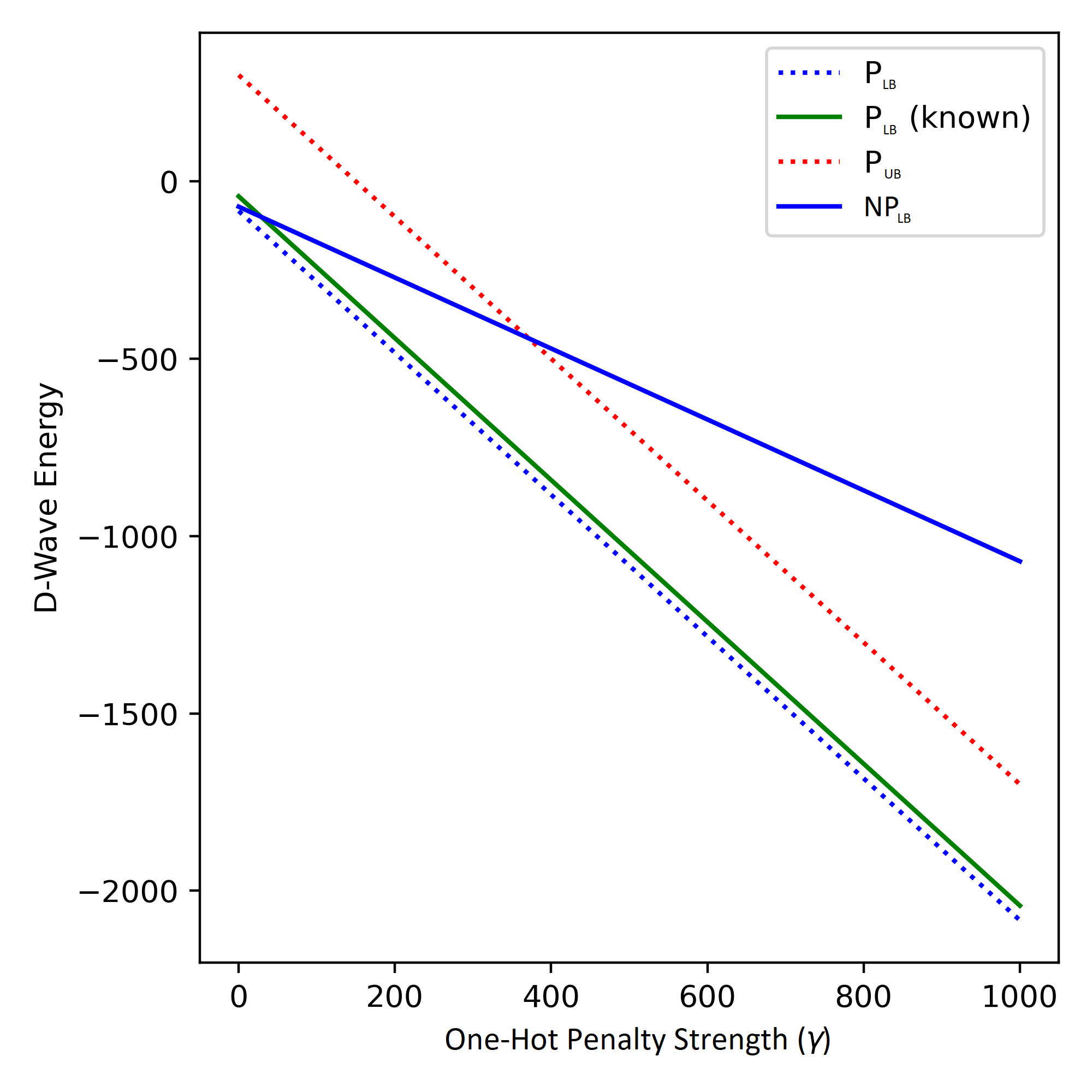
Figure A.1: Predicted physical and non-physical state distribution energy bounds for three helix bundle (PDB ID: 4TQL) over a simulation-space confined to an $xy-$plane. The corresponding pairwise energy file was found to have a minimum pairwise interaction energy of $-38.83$ Rosetta Energy Units (REU), maximum pairwise interaction energy of $100.00$ REU, and a mean pairwise interaction energy of $22.26$ REU. Empirically, we have seen that the non-physical lower bound crosses the physical lower bound at $\gamma>0$, in contrast to prediction, but we do correctly predict that energy separation between physical and non-physical states occurs when $100\leq\gamma\leq 1000$.

We suggest this approach as a guide to determine where separation between physical and non-physical states occurs, and approximate degrees of energy mixing. One simplifying assumption we made took each minimum pairwise interaction energy between any two bodies to be identical (based on the absolute minimum of this set of energies), but it is possible to use the actual minimum pairwise energies between any two bodies.

Appendix B Solution diversity

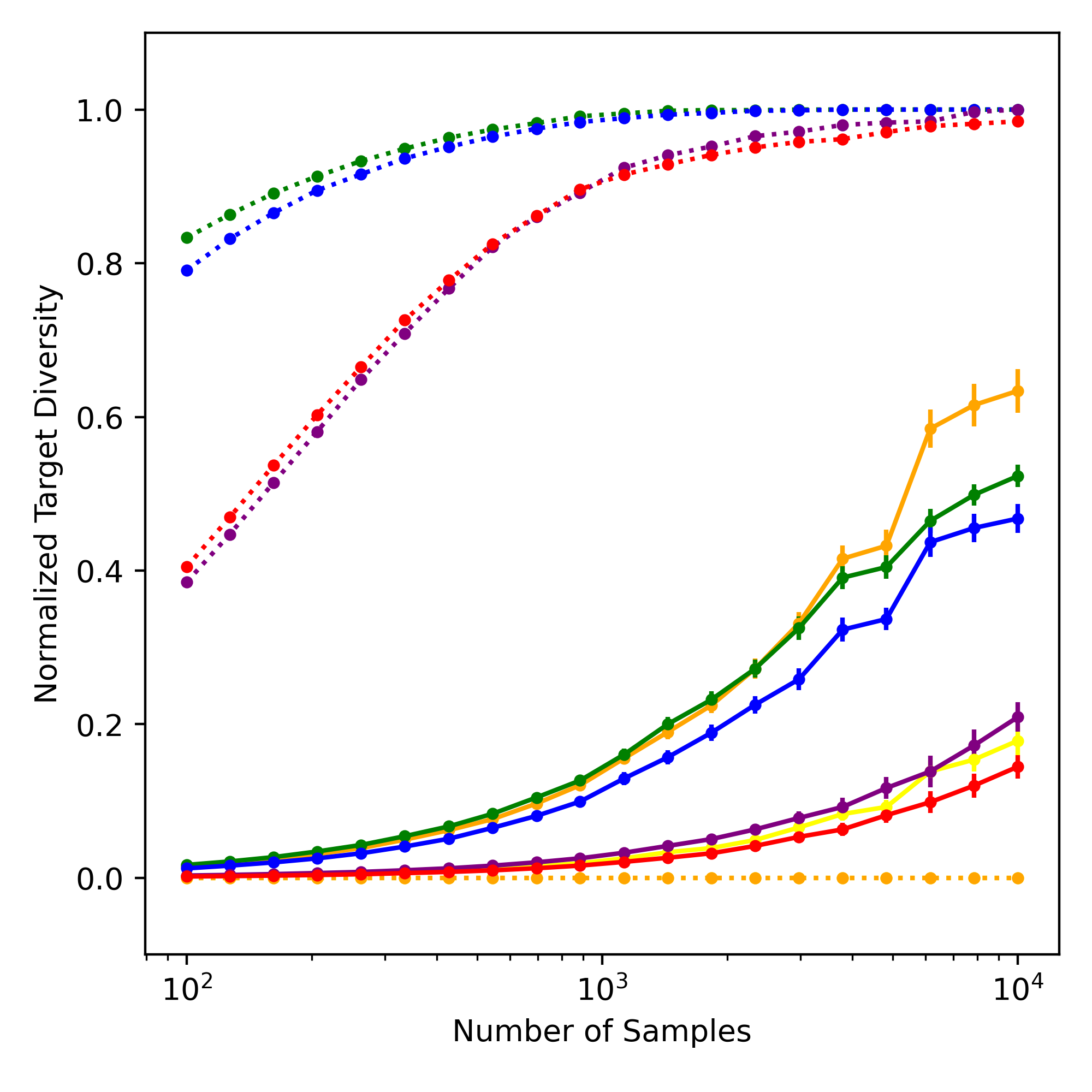
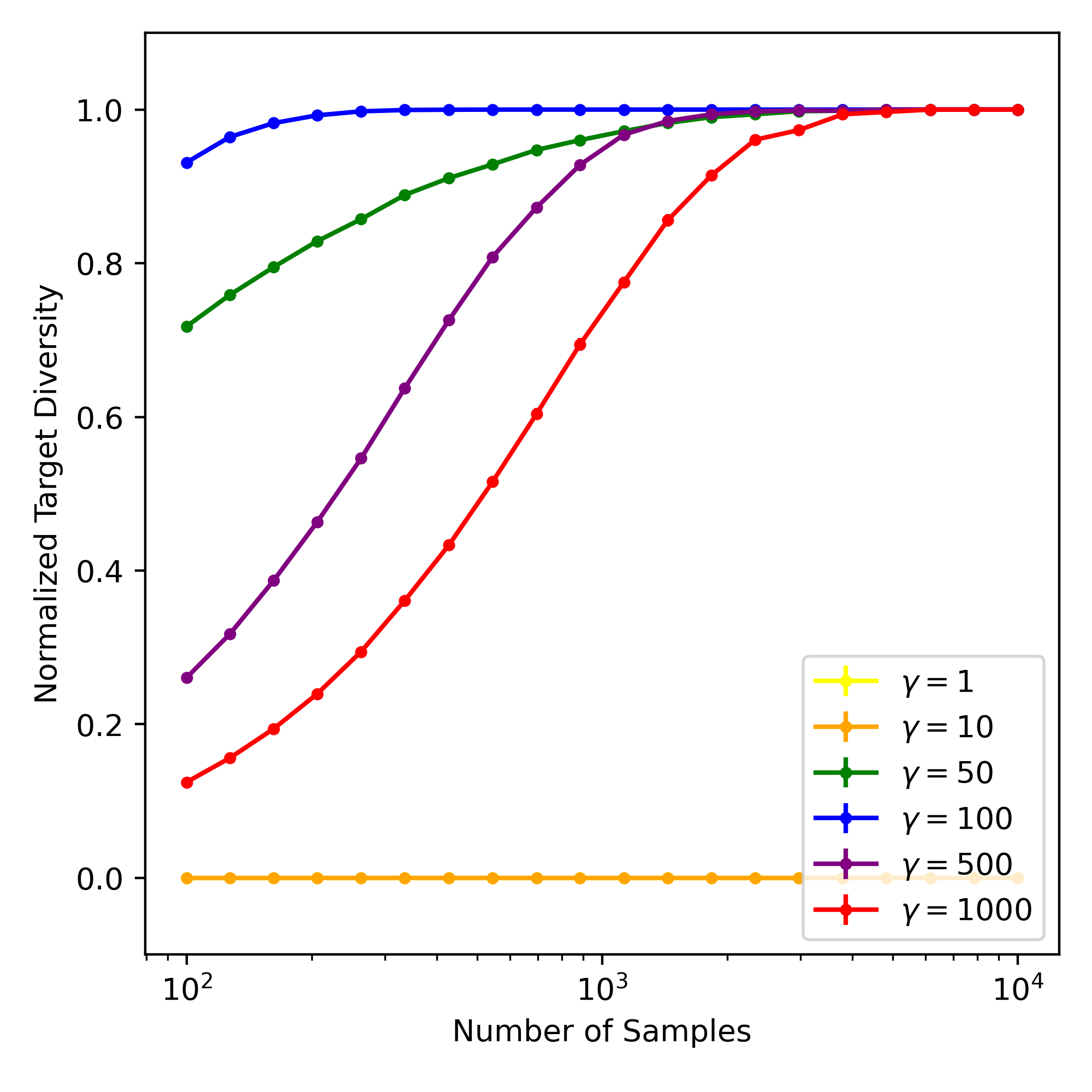
Figure A.2: Average normalized target diversity (left panel) returned by D-Wave Advantage 4.1 of one-hot three helix bundle QUBO as a function of number of samples. Each point registers the mean of $25\cdot 10^{4}/n$ replicates, where $n$ is the number of samples. Solid curves correspond to diversity prior to steepest descent post-processing (NG for non-greedy); dotted curves correspond to diversity with steepest descent post-processing (G for greedy). Non-greedy curves show better diversity for $1\leq\gamma\leq 100$, while greedy curves show better diversity for $50\leq\gamma\leq 100$. Greedy post-processing when $\gamma<50$ takes all solutions to non-physical states (zero diversity). The right panel shows average normalized diversity returned by the QUBO simulated annealing solver. Notice that for $\gamma=100$ diversity is most quickly reached, and for $\gamma<50$, all solutions are non-physical.

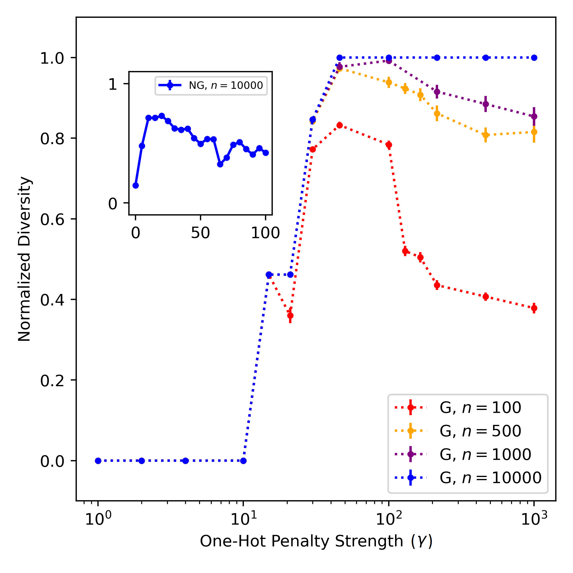
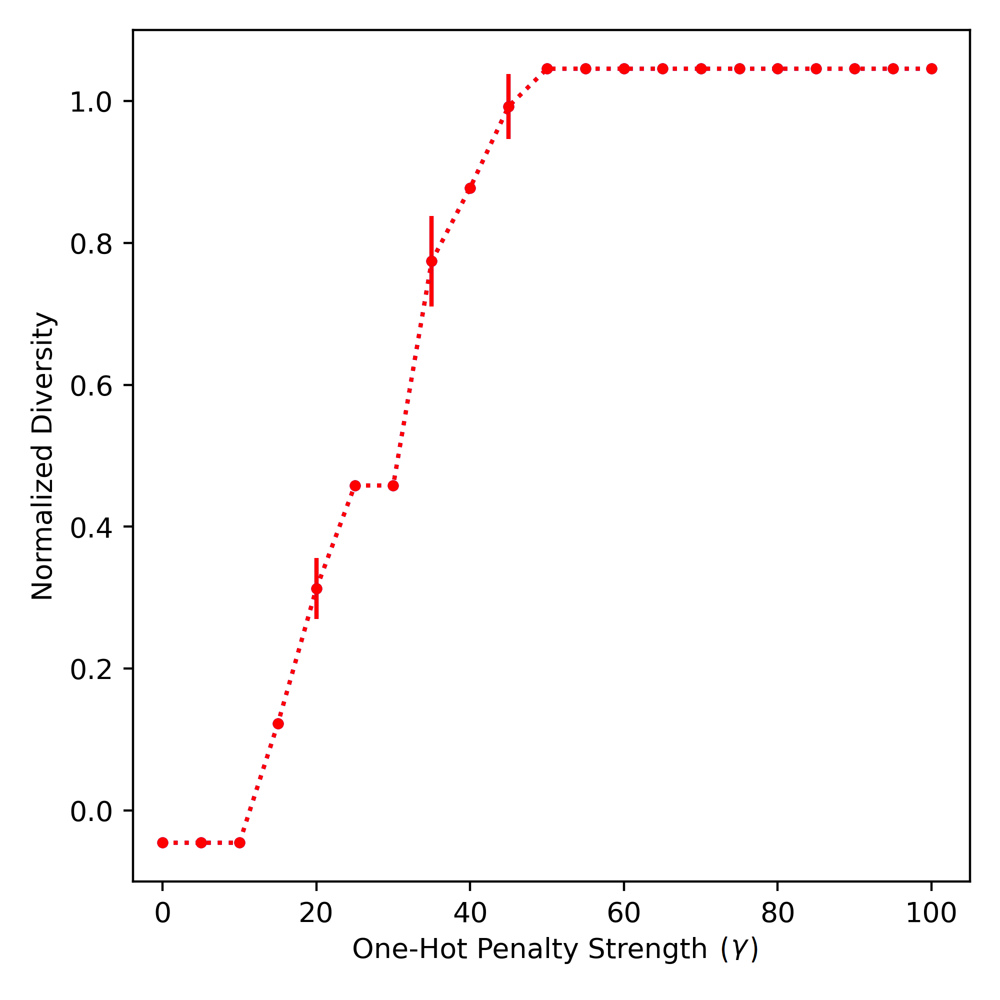
Figure A.3: Average normalized diversity returned by D-Wave Advantage 4.1 of one-hot three helix bundle QUBO as a function of one-hot penalty strength (left panel). Each point registers the average of $10^{4}/n$ replicates of $n$ samples. Highest diversity is achieved for $\gamma\geq 50$ with greedy post-processing, and zero diversity for $\gamma\leq 10$, where all solutions are taken to non-physical states. The inset shows non-greedy average normalized diversity as a function of penalty strength, with 30 replicates of $10^{4}$ samples per point. Diversity peaks when $\gamma=10$. The right panel shows average normalized diversity returned by the QUBO simulated annealing sampler over 30 replicates of $10^{4}$ samples as a function of one-hot penalty strength. For $\gamma\geq 50$, full diversity is achieved.

Appendix C Solution quality

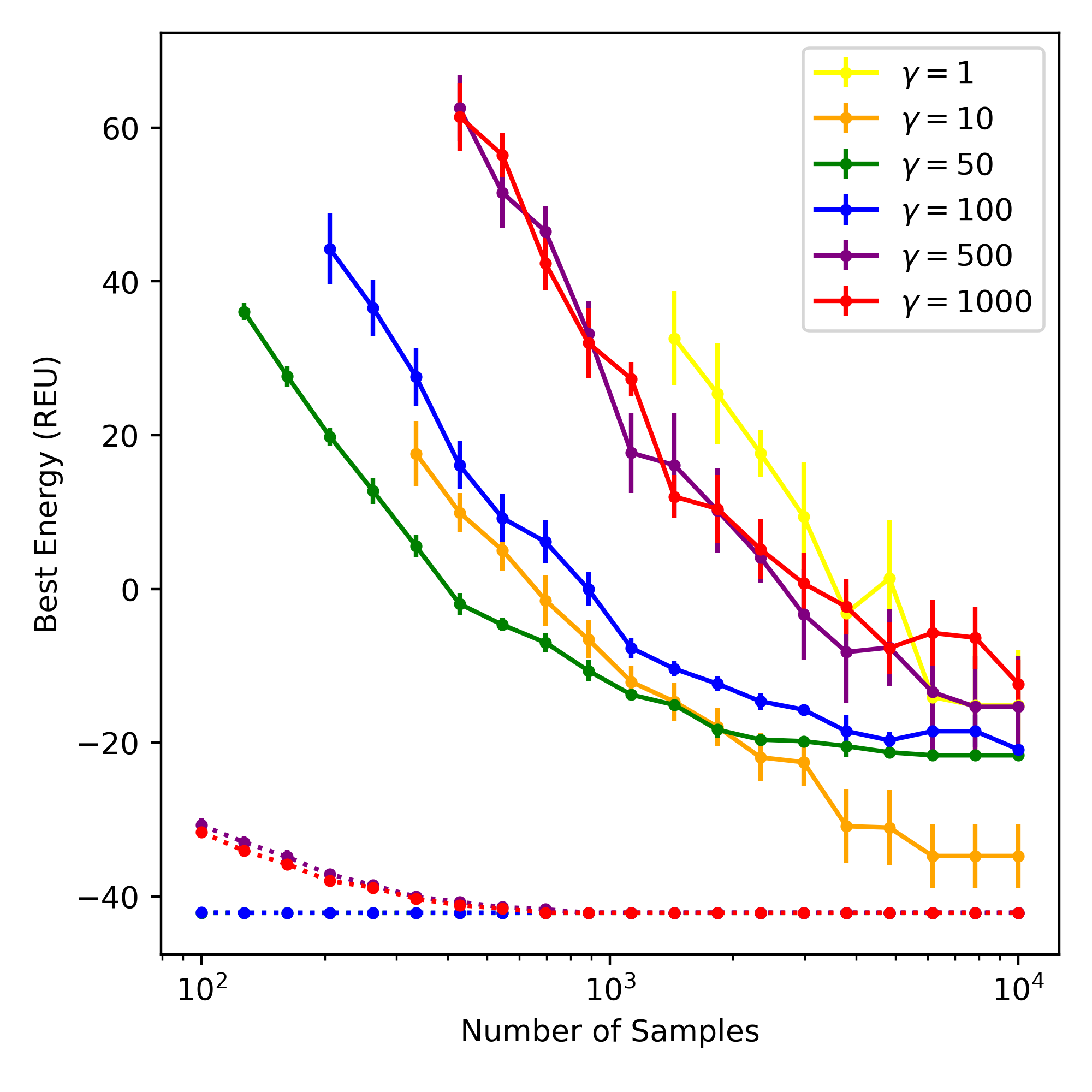
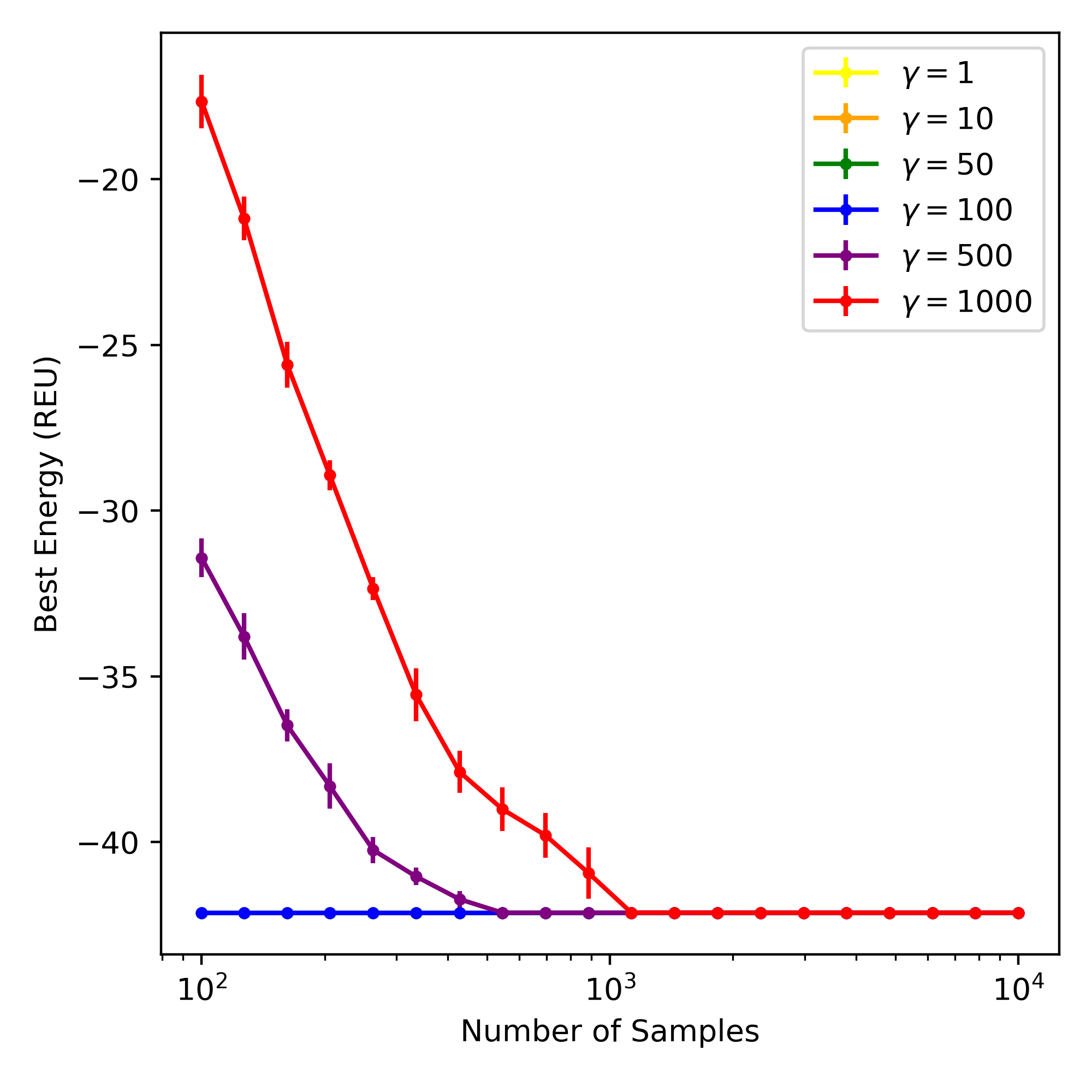
Figure A.4: Best energy returned by D-Wave Advantage 4.1 of one-hot three helix bundle QUBO as a function of number of samples (left panel). Each point registers the mean of $25\cdot 10^{4}/n$ replicates, where $n$ is the number of samples. Solid curves correspond to diversity prior to steepest descent post-processing (NG for non-greedy); dotted curves correspond to diversity with steepest descent post-processing (G for greedy). Non-greedy curves show better best energy for $10\leq\gamma\leq 100$, while greedy curves show improved best energy for $\gamma\geq 100$. Greedy post-processing when $\gamma\leq 10$ takes all solutions to non-physical states (zero diversity, no best energy). The right panel shows best energy found by the QUBO simulated annealing solver. For $\gamma\leq 10$ all solutions are non-physical; $50\leq\gamma\leq 100$ shows best performance.

References

- (1) G. Sliwoski, S. Kothiwale, J. Meiler, and E. W. Lowe, “Computational methods in drug discovery,” Pharmacological reviews, vol. 66, no. 1, pp. 334–395, 2014.
- (2) V. K. Mulligan, “The emerging role of computational design in peptide macrocycle drug discovery,” Expert Opinion on Drug Discovery, vol. 15, no. 7, pp. 833–852, 2020.
- (3) Y. Cao, J. Romero, and A. Aspuru-Guzik, “Potential of quantum computing for drug discovery,” IBM Journal of Research and Development, vol. 62, no. 6, pp. 6–1, 2018.
- (4) C. Outeiral, M. Strahm, J. Shi, G. M. Morris, S. C. Benjamin, and C. M. Deane, “The prospects of quantum computing in computational molecular biology,” Wiley Interdisciplinary Reviews: Computational Molecular Science, vol. 11, no. 1, p. e1481, 2021.
- (5) M. Zinner, F. Dahlhausen, P. Boehme, J. Ehlers, L. Bieske, and L. Fehring, “Quantum computing’s potential for drug discovery: Early stage industry dynamics,” Drug Discovery Today, vol. 26, no. 7, pp. 1680–1688, 2021.
- (6) L. Banchi, M. Fingerhuth, T. Babej, C. Ing, and J. M. Arrazola, “Molecular docking with gaussian boson sampling,” Science advances, vol. 6, no. 23, p. eaax1950, 2020.
- (7) V. K. Mulligan, H. Melo, H. I. Merritt, S. Slocum, B. D. Weitzner, A. M. Watkins, P. D. Renfrew, C. Pelissier, P. S. Arora, and R. Bonneau, “Designing peptides on a quantum computer,” BioRxiv, 2020.
- (8) K. Mato, R. Mengoni, D. Ottaviani, and G. Palermo, “Quantum molecular unfolding,” Quantum Science and Technology, 2022.
- (9) P. A. M. Casares, R. Campos, and M. A. Martin-Delgado, “Qfold: quantum walks and deep learning to solve protein folding,” Quantum Science and Technology, vol. 7, no. 2, p. 025013, 2022.
- (10) J. Tilly, H. Chen, S. Cao, D. Picozzi, K. Setia, Y. Li, E. Grant, L. Wossnig, I. Rungger, G. H. Booth et al., “The variational quantum eigensolver: a review of methods and best practices,” arXiv preprint arXiv:2111.05176, 2021.
- (11) Y. Cao, J. Romero, J. P. Olson, M. Degroote, P. D. Johnson, M. Kieferová, I. D. Kivlichan, T. Menke, B. Peropadre, N. P. Sawaya et al., “Quantum chemistry in the age of quantum computing,” Chemical reviews, vol. 119, no. 19, pp. 10 856–10 915, 2019.
- (12) K. Batra, K. M. Zorn, D. H. Foil, E. Minerali, V. O. Gawriljuk, T. R. Lane, and S. Ekins, “Quantum machine learning algorithms for drug discovery applications,” Journal of chemical information and modeling, vol. 61, no. 6, pp. 2641–2647, 2021.
- (13) J. Li, M. Alam, M. S. Congzhou, J. Wang, N. V. Dokholyan, and S. Ghosh, “Drug discovery approaches using quantum machine learning,” in 2021 58th ACM/IEEE Design Automation Conference (DAC). IEEE, 2021, pp. 1356–1359.
- (14) J. Preskill, “Quantum computing in the nisq era and beyond,” Quantum, vol. 2, p. 79, 2018.
- (15) N. Moll, P. Barkoutsos, L. S. Bishop, J. M. Chow, A. Cross, D. J. Egger, S. Filipp, A. Fuhrer, J. M. Gambetta, M. Ganzhorn, A. Kandala, A. Mezzacapo, P. Müller, W. Riess, G. Salis, J. Smolin, I. Tavernelli, and K. Temme, “Quantum optimization using variational algorithms on near-term quantum devices,” Quantum Science and Technology, vol. 3, no. 3, p. 030503, 2018.
- (16) S. Kirkpatrick, C. D. Gelatt Jr, and M. P. Vecchi, “Optimization by simulated annealing,” science, vol. 220, no. 4598, pp. 671–680, 1983.
- (17) V. Černỳ, “Thermodynamical approach to the traveling salesman problem: An efficient simulation algorithm,” Journal of optimization theory and applications, vol. 45, no. 1, pp. 41–51, 1985.
- (18) S. Geman and D. Geman, “Stochastic relaxation, gibbs distributions, and the bayesian restoration of images,” IEEE Transactions on pattern analysis and machine intelligence, no. 6, pp. 721–741, 1984.
- (19) B. Suman and P. Kumar, “A survey of simulated annealing as a tool for single and multiobjective optimization,” Journal of the operational research society, vol. 57, no. 10, pp. 1143–1160, 2006.
- (20) F. Romeo and A. Sangiovanni-Vincentelli, “A theoretical framework for simulated annealing,” Algorithmica, vol. 6, no. 1, pp. 302–345, 1991.
- (21) J. Jumper, R. Evans, A. Pritzel, T. Green, M. Figurnov, O. Ronneberger, K. Tunyasuvunakool, R. Bates, A. Žídek, A. Potapenko, A. Bridgland, C. Meyer, S. A. A. Kohl, A. J. Ballard, A. Cowie, B. Romera-Paredes, S. Nikolov, R. Jain, J. Adler, T. Back, S. Petersen, D. Reiman, E. Clancy, M. Zielinski, M. Steinegger, M. Pacholska, T. Berghammer, S. Bodenstein, D. Silver, O. Vinyals, A. W. Senior, K. Kavukcuoglu, P. Kohli, and D. Hassabis, “Highly accurate protein structure prediction with AlphaFold,” Nature, vol. 596, no. 7873, pp. 583–589, Aug. 2021, number: 7873 Publisher: Nature Publishing Group.
- (22) M. Källberg, H. Wang, S. Wang, J. Peng, Z. Wang, H. Lu, and J. Xu, “Template-based protein structure modeling using the RaptorX web server,” Nature Protocols, vol. 7, no. 8, pp. 1511–1522, Aug. 2012, number: 8 Publisher: Nature Publishing Group.
- (23) S. Ovchinnikov, H. Park, D. E. Kim, F. DiMaio, and D. Baker, “Protein structure prediction using Rosetta in CASP12,” Proteins, vol. 86, no. Suppl 1, pp. 113–121, Mar. 2018.
- (24) A. Leaver-Fay, M. Tyka, S. M. Lewis, O. F. Lange, J. Thompson, R. Jacak, K. W. Kaufman, P. D. Renfrew, C. A. Smith, W. Sheffler, I. W. Davis, S. Cooper, A. Treuille, D. J. Mandell, F. Richter, Y.-E. A. Ban, S. J. Fleishman, J. E. Corn, D. E. Kim, S. Lyskov, M. Berrondo, S. Mentzer, Z. Popović, J. J. Havranek, J. Karanicolas, R. Das, J. Meiler, T. Kortemme, J. J. Gray, B. Kuhlman, D. Baker, and P. Bradley, “Rosetta3,” in Methods in Enzymology. Elsevier, 2011, vol. 487, pp. 545–574.
- (25) E.-M. Strauch, S. M. Bernard, D. La, A. J. Bohn, P. S. Lee, C. E. Anderson, T. Nieusma, C. A. Holstein, N. K. Garcia, K. A. Hooper, R. Ravichandran, J. W. Nelson, W. Sheffler, J. D. Bloom, K. K. Lee, A. B. Ward, P. Yager, D. H. Fuller, I. A. Wilson, and D. Baker, “Computational design of trimeric influenza-neutralizing proteins targeting the hemagglutinin receptor binding site,” Nature Biotechnology, vol. 35, no. 7, pp. 667–671, Jul. 2017.
- (26) V. K. Mulligan, S. Workman, T. Sun, S. Rettie, X. Li, L. J. Worrall, T. W. Craven, D. T. King, P. Hosseinzadeh, A. M. Watkins, P. D. Renfrew, S. Guffy, J. W. Labonte, R. Moretti, R. Bonneau, N. C. J. Strynadka, and D. Baker, “Computationally designed peptide macrocycle inhibitors of New Delhi metallo--lactamase 1,” Proceedings of the National Academy of Sciences of the United States of America, vol. 118, no. 12, p. e2012800118, Mar. 2021.
- (27) P. Hosseinzadeh, P. R. Watson, T. W. Craven, X. Li, S. Rettie, F. Pardo-Avila, A. K. Bera, V. K. Mulligan, P. Lu, A. S. Ford, B. D. Weitzner, L. J. Stewart, A. P. Moyer, M. Di Piazza, J. G. Whalen, P. J. Greisen, D. W. Christianson, and D. Baker, “Anchor extension: a structure-guided approach to design cyclic peptides targeting enzyme active sites,” Nature Communications, vol. 12, no. 1, p. 3384, Jun. 2021.
- (28) Y. Li, V. A. Protopopescu, and A. Gorin, “Accelerated simulated tempering,” Physics letters A, vol. 328, no. 4-5, pp. 274–283, 2004.
- (29) Y. Li, C. E. Strauss, and A. Gorin, “Parallel tempering in rosetta practice,” in Advances in Bioinformatics and Its Applications. World Scientific, 2005, pp. 380–389.
- (30) A. Das and B. K. Chakrabarti, “Colloquium: Quantum annealing and analog quantum computation,” Reviews of Modern Physics, vol. 80, no. 3, p. 1061, 2008.
- (31) T. F. Rønnow, Z. Wang, J. Job, S. Boixo, S. V. Isakov, D. Wecker, J. M. Martinis, D. A. Lidar, and M. Troyer, “Defining and detecting quantum speedup,” science, vol. 345, no. 6195, pp. 420–424, 2014.
- (32) B. Heim, T. F. Rønnow, S. V. Isakov, and M. Troyer, “Quantum versus classical annealing of ising spin glasses,” Science, vol. 348, no. 6231, pp. 215–217, 2015.
- (33) V. S. Denchev, S. Boixo, S. V. Isakov, N. Ding, R. Babbush, V. Smelyanskiy, J. Martinis, and H. Neven, “What is the computational value of finite-range tunneling?” Physical Review X, vol. 6, no. 3, p. 031015, 2016.
- (34) R. Das and D. Baker, “Macromolecular modeling with rosetta,” Annual review of biochemistry, vol. 77, no. 1, pp. 363–382, 2008.
- (35) K. W. Kaufmann, G. H. Lemmon, S. L. DeLuca, J. H. Sheehan, and J. Meiler, “Practically useful: what the rosetta protein modeling suite can do for you,” Biochemistry, vol. 49, no. 14, pp. 2987–2998, 2010.
- (36) R. F. Alford, A. Leaver-Fay, J. R. Jeliazkov, M. J. O’Meara, F. P. DiMaio, H. Park, M. V. Shapovalov, P. D. Renfrew, V. K. Mulligan, K. Kappel et al., “The rosetta all-atom energy function for macromolecular modeling and design,” Journal of chemical theory and computation, vol. 13, no. 6, pp. 3031–3048, 2017.
- (37) J. K. Leman, B. D. Weitzner, S. M. Lewis, J. Adolf-Bryfogle, N. Alam, R. F. Alford, M. Aprahamian, D. Baker, K. A. Barlow, P. Barth et al., “Macromolecular modeling and design in rosetta: recent methods and frameworks,” Nature methods, vol. 17, no. 7, pp. 665–680, 2020.
- (38) M. A. Hallen, J. W. Martin, A. Ojewole, J. D. Jou, A. U. Lowegard, M. S. Frenkel, P. Gainza, H. M. Nisonoff, A. Mukund, S. Wang et al., “Osprey 3.0: open-source protein redesign for you, with powerful new features,” Journal of computational chemistry, vol. 39, no. 30, pp. 2494–2507, 2018.
- (39) S. Patel and C. L. Brooks, “CHARMM fluctuating charge force field for proteins: I parameterization and application to bulk organic liquid simulations,” Journal of Computational Chemistry, vol. 25, no. 1, pp. 1–16, Jan. 2004.
- (40) J. Huang, S. Rauscher, G. Nawrocki, T. Ran, M. Feig, B. L. d. Groot, H. Grubmüller, and A. D. MacKerell, “CHARMM36m: an improved force field for folded and intrinsically disordered proteins,” Nature Methods, vol. 14, no. 1, pp. 71–73, Jan. 2017.
- (41) J. Wang, R. M. Wolf, J. W. Caldwell, P. A. Kollman, and D. A. Case, “Development and testing of a general amber force field,” Journal of Computational Chemistry, vol. 25, no. 9, pp. 1157–1174, Jul. 2004.
- (42) J. A. Maier, C. Martinez, K. Kasavajhala, L. Wickstrom, K. E. Hauser, and C. Simmerling, “ff14SB: Improving the Accuracy of Protein Side Chain and Backbone Parameters from ff99SB,” Journal of Chemical Theory and Computation, vol. 11, no. 8, pp. 3696–3713, Aug. 2015.
- (43) P. M. Dean and R. A. Lewis, Molecular diversity in drug design. Springer, 1999.
- (44) W. R. Galloway, A. Isidro-Llobet, and D. R. Spring, “Diversity-oriented synthesis as a tool for the discovery of novel biologically active small molecules,” Nature communications, vol. 1, no. 1, pp. 1–13, 2010.
- (45) D. Gorse, A. Rees, M. Kaczorek, and R. Lahana, “Molecular diversity and its analysis,” Drug Discovery Today, vol. 4, no. 6, pp. 257–264, 1999.
- (46) D. J. Huggins, A. R. Venkitaraman, and D. R. Spring, “Rational methods for the selection of diverse screening compounds,” ACS chemical biology, vol. 6, no. 3, pp. 208–217, 2011.
- (47) J. King, S. Yarkoni, J. Raymond, I. Ozfidan, A. D. King, M. M. Nevisi, J. P. Hilton, and C. C. McGeoch, “Quantum annealing amid local ruggedness and global frustration,” Journal of the Physical Society of Japan, vol. 88, no. 6, p. 061007, 2019.
- (48) M. Mohseni, M. M. Rams, S. V. Isakov, D. Eppens, S. Pielawa, J. Strumpfer, S. Boixo, and H. Neven, “Diversity measure for discrete optimization: Sampling rare solutions via algorithmic quantum annealing,” arXiv preprint arXiv:2110.10560, 2021.
- (49) A. Zucca, H. Sadeghi, M. Mohseni, and M. H. Amin, “Diversity metric for evaluation of quantum annealing,” arXiv preprint arXiv:2110.10196, 2021.
- (50) X.-Y. Meng, H.-X. Zhang, M. Mezei, and M. Cui, “Molecular docking: a powerful approach for structure-based drug discovery,” Current computer-aided drug design, vol. 7, no. 2, pp. 146–157, 2011.
- (51) W. Xiao, D. Wang, Z. Shen, S. Li, and H. Li, “Multi-body interactions in molecular docking program devised with key water molecules in protein binding sites,” Molecules, vol. 23, no. 9, p. 2321, 2018.
- (52) C. W. van Noort, R. V. Honorato, and A. M. Bonvin, “Information-driven modeling of biomolecular complexes,” Current Opinion in Structural Biology, vol. 70, pp. 70–77, 2021.
- (53) S. A. Combs, S. L. DeLuca, S. H. DeLuca, G. H. Lemmon, D. P. Nannemann, E. D. Nguyen, J. R. Willis, J. H. Sheehan, and J. Meiler, “Small-molecule ligand docking into comparative models with rosetta,” Nature protocols, vol. 8, no. 7, pp. 1277–1298, 2013.
- (54) S. DeLuca, K. Khar, and J. Meiler, “Fully flexible docking of medium sized ligand libraries with rosettaligand,” PLOS one, vol. 10, no. 7, p. e0132508, 2015.
- (55) M. F. Perutz, M. G. Rossmann, A. F. Cullis, H. Muirhead, G. Will, and A. C. North, “Structure of haemoglobin: a three-dimensional Fourier synthesis at 5.5-A. resolution, obtained by X-ray analysis,” Nature, vol. 185, no. 4711, pp. 416–422, Feb. 1960.
- (56) M. H. Ali and B. Imperiali, “Protein oligomerization: how and why,” Bioorganic & Medicinal Chemistry, vol. 13, no. 17, pp. 5013–5020, Sep. 2005.
- (57) B. C. Roberts and R. L. Mancera, “Ligand- protein docking with water molecules,” Journal of chemical information and modeling, vol. 48, no. 2, pp. 397–408, 2008.
- (58) M. Rosell and J. Fernández-Recio, “Docking approaches for modeling multi-molecular assemblies,” Current opinion in structural biology, vol. 64, pp. 59–65, 2020.
- (59) E. Karaca, A. S. Melquiond, S. J. De Vries, P. L. Kastritis, and A. M. Bonvin, “Building macromolecular assemblies by information-driven docking,” Molecular & Cellular Proteomics, vol. 9, no. 8, pp. 1784–1794, 2010.
- (60) S. J. de Vries, C. E. Schindler, I. C. de Beauchêne, and M. Zacharias, “A web interface for easy flexible protein-protein docking with attract,” Biophysical journal, vol. 108, no. 3, pp. 462–465, 2015.
- (61) S. J. de Vries and M. Zacharias, “Attract-em: a new method for the computational assembly of large molecular machines using cryo-em maps,” PLOS one, vol. 7, no. 12, p. e49733, 2012.
- (62) M. E. Ruiz Echartea, D. W. Ritchie, and I. Chauvot de Beauchêne, “Using restraints in eros-dock improves model quality in pairwise and multicomponent protein docking,” Proteins: Structure, Function, and Bioinformatics, vol. 88, no. 8, pp. 1121–1128, 2020.
- (63) H. Li and C. Li, “Multiple ligand simultaneous docking: orchestrated dancing of ligands in binding sites of protein,” Journal of computational chemistry, vol. 31, no. 10, pp. 2014–2022, 2010.
- (64) J. Chen, T. Stollenwerk, and N. Chancellor, “Performance of domain-wall encoding for quantum annealing,” IEEE Transactions on Quantum Engineering, vol. 2, pp. 1–14, 2021.
- (65) N. Chancellor, “Domain wall encoding of discrete variables for quantum annealing and QAOA,” Quantum Science and Technology, vol. 4, no. 4, p. 045004, 2019.
- (66) V. Kumar, G. Bass, C. Tomlin, and J. Dulny, “Quantum annealing for combinatorial clustering,” Quantum Information Processing, vol. 17, no. 2, pp. 1–14, 2018.
- (67) E. G. Rieffel, D. Venturelli, B. O’Gorman, M. B. Do, E. M. Prystay, and V. N. Smelyanskiy, “A case study in programming a quantum annealer for hard operational planning problems,” Quantum Information Processing, vol. 14, no. 1, pp. 1–36, 2015.
- (68) T. Stollenwerk, E. Lobe, and M. Jung, “Flight gate assignment with a quantum annealer,” in International Workshop on Quantum Technology and Optimization Problems. Springer, 2019, pp. 99–110.
- (69) A. Lucas, “Ising formulations of many NP problems,” Frontiers in physics, p. 5, 2014.
- (70) M. Born and V. Fock, “Beweis des Adiabatensatzes,” Zeitschrift für Physik, vol. 51, no. 3-4, pp. 165–180, Mar. 1928.
- (71) H. Park, P. Bradley, P. Greisen, Y. Liu, V. K. Mulligan, D. E. Kim, D. Baker, and F. DiMaio, “Simultaneous Optimization of Biomolecular Energy Functions on Features from Small Molecules and Macromolecules,” Journal of Chemical Theory and Computation, vol. 12, no. 12, pp. 6201–6212, Dec. 2016.
- (72) P.-S. Huang, G. Oberdorfer, C. Xu, X. Y. Pei, B. L. Nannenga, J. M. Rogers, F. DiMaio, T. Gonen, B. Luisi, and D. Baker, “High thermodynamic stability of parametrically designed helical bundles,” Science (New York, N.Y.), vol. 346, no. 6208, pp. 481–485, Oct. 2014.
- (73) C. McGeoch and P. Farré, “The advantage system: Performance update,” D-Wave, Tech. Rep., 10 2021. [Online]. Available: https://www.dwavesys.com/media/kjtlcemb/14-1054a-a_advantage_system_performance_update.pdf
- (74) “Error sources for problem representation,” accessed: 2022-10-11. [Online]. Available: https://docs.dwavesys.com/docs/latest/c_qpu_ice.html