Attention-based Modeling of Physical Systems: Improved Latent Representations

Abstract

We propose attention-based modeling of quantities at arbitrary spatial points conditioned on related measurements at different locations. Our approach adapts a transformer-encoder to process measurements and read-out positions together. Attention-based models exhibit excellent performance across domains, which makes them an interesting candidate for modeling data irregularly sampled in space. We introduce a novel encoding strategy that applies the same transformation to the measurements and read-out positions, after which they are combined with encoded measurement values instead of relying on two different mappings. Efficiently learning input-output mappings from irregularly-spaced data is a fundamental challenge in modeling physical phenomena. To evaluate the effectiveness of our model, we conduct experiments on diverse problem domains, including high-altitude wind nowcasting, two-days weather forecasting, fluid dynamics, and heat diffusion. Our attention-based model consistently outperforms state-of-the-art models, such as Graph Element Networks and Conditional Neural Processes, for modeling irregularly sampled data. Notably, our model reduces root mean square error (RMSE) for wind nowcasting, improving from 9.24 to 7.98 and for a heat diffusion task from .126 to .084. We hypothesize that this superior performance can be attributed to the enhanced flexibility of our latent representation and the improved data encoding technique. To support our hypothesis, we design a synthetic experiment that reveals excessive bottlenecking in the latent representations of alternative models, which hinders information utilization and impedes training.

1 Introduction

Deep learning (DL) has emerged as a powerful tool for modeling dynamical system in recent years, leveraging vast amounts of data available in ways that traditional solvers cannot. This has led to a growing reliance on DL models in weather forecasting, with state-of-the-art results in precipitation nowcasting [25, 24] and performance on par with traditional partial differential equation (PDE) solvers in medium-term forecasting [15]. However, these applications are currently limited to data represented as images or on regular grids, where models such as convolutional networks or graph neural networks are used. In contrast, various real-world data like flight recorded data is often irregularly sampled in space, which means custom architectures are needed to handle it effectively.

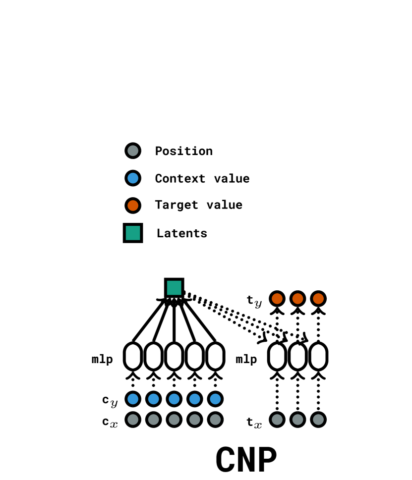
(a) Conditional Neural Processes [7]

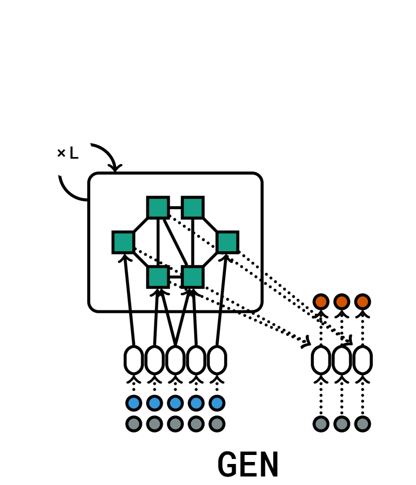
(b) Graph Element Networks [1]

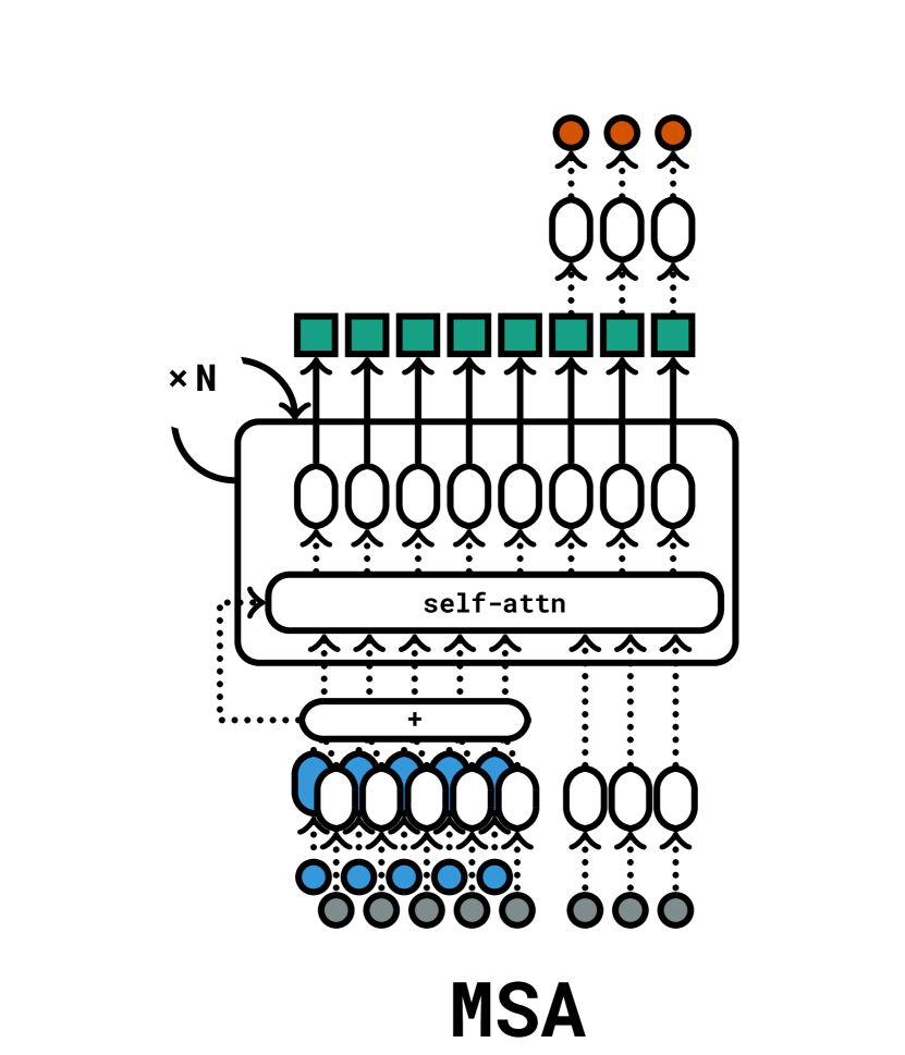
(c) Multi-layer Self Attention (Ours)

Figure 1: Illustration of the different models for modeling irregularly-spaced data compared in this work. Each model encodes a context ($\mathbf{c}_{x},\mathbf{c}_{y}$), utilizes its latent representation to decode a target position $\mathbf{t}_{x}$ into a forecast $\mathbf{t}_{y}$. In the diagram mlp refers to per-token multi-layer perceptron, while self-attn represents self-attention layers. GEN process the latents by applying $L$ layer of message-passing. MSA shares the same mlp for both context and target positions and it processes both context and target inputs at the same time through $N$ blocks of self-attention followed by multi-layer perceptrons.

Building upon this need for a more flexible deep learning approach, we turn our attention toward the field of air traffic control (ATC). ATC requires reliable weather forecasts to manage airspace efficiently. This is particularly true for wind conditions, as planes are highly sensitive to wind and deviations from the initial flight plan can be costly and pose safety hazards. DL models are a promising candidate to produce reliable wind forecasts as a large amount of data is collected from airplanes that broadcast wind speed measurements with a recording frequency of around four seconds. To effectively model wind nowcasting using data collected from airplanes, we require a model that can encode recent measurements such that the order of contemporary measurements in a context of recent data should not impact the prediction. The model must also be able to decode anywhere in space, as we aim to predict wind conditions at future locations of the airplane, based on past measurements taken by that specific airplane or neighboring ones.

To meet these requirements, we introduce a Multi-layer Self-Attention model (MSA) and compare it to two different baselines: Conditional Neural Processes (CNP) [7] and Graph Element Networks (GEN) [1]. While all of these models possess the aforementioned characteristics, they each adopt distinct strategies for representing measurements within the latent space. CNP models use a single vector as a summary of encoded measures, while GEN models map the context to a graph, based on their distance to its nodes. MSA keep one latent vector per encoded measurement and can access them directly for forecasting. This latent representation is better, as it does not create a bottleneck. We show that due to that architectural choice, both baselines can fail, in certain cases, to retrieve information present in the context they condition on.

Our approach offers better performance than its competitors and is conceptually simpler as it does not require an encoder-decoder structure. To evaluate the effectiveness of our approach, we conducted experiments on high-altitude wind nowcasting, heat diffusion and fluid dynamics and two-day weather nowcasting. Several additional ablations studies show the impact of different architectural choices.

The main contributions of this work are summarized below:

• We develop an attention-based model that can generate prediction anywhere in the space conditioned on a set of measurements.

• We evaluate our method on a set of challenging tasks with data irregularly sampled in space: high-altitude wind nowcasting, two-day weather forecasting, heat diffusion and fluid dynamics.

• We examine the differences between models, and explain the impact of design choices such as latent representation bottlenecks on the final performance of the trained models.

• We propose a novel encoding scheme using a shared MLP encoder to map context and target positions, improving forecasting performance and enhancing the model’s understanding of spatial patterns.

2 Related works

DL performance for weather nowcasting has improved in recent years, with DL models increasingly matching or surpassing the performance of traditional PDE-based systems. Initially applied to precipitation nowcasting based on 2D radar images [25, 24], DL-based models have recently surpassed traditional methods for longer forecast periods [15]. In the case of radar precipitation, data is organized as images and convolutional neural networks are utilized. For 3D regular spherical grid data, graph neural networks are employed [15]. However, in our study, the dataset is distributed sparsely in space, which hinders the use of these traditional architectures. The use of DL for modelling dynamical systems in general has also seen recent advancements [18, 10, 21] for similar reasons as in weather forecasting. However, most approaches in this field also typically operate on regularly-spaced data as well.

Neural Processes [7, 14], Graph Element Networks [1] and attention-based models [26] are three DL-based approaches that are capable of modeling sets of data. In this study, we conduct a comparison of these models by selecting a representative architecture from each category. Additionally, attention-based models have been previously adapted for set classification tasks [16], and here we adapt them to generate forecasts.

Pannatier et al. [20] use a kernel-based method for wind nowcasting based on flight data. This method incorporates a distance metric with learned parameters to combine contexts for prediction at any spatial location. However, a notable limitation of this technique is that its forecasts are constrained to the convex hull of the input measurements, preventing accurate extrapolation. We evaluate the efficacy of our method compared to this approach, along with the distinct outcomes obtained, in section 10 of the supplementary material.

Our work builds upon well-established attention models, which have demonstrated their versatility and efficacy in various domains. Although the core model is essentially a vanilla transformer, our architecture required careful adaptation to suit our specific requirements. We designed our model to be set-to-set rather than sequence-to-sequence, handling data in a non-causal and non-autoregressive manner, and generating continuous values for regression. The success of influential models like BERT [4], GPT [22], ViT [5], and Whisper [23], also closely resemble the original implementation by Vaswani et al. [26], further supports the effectiveness of the transformer framework across different tasks and domains. It is worth noting that a vast review of different modifications of the transformer architecture [19] suggests its remarkable robustness, making it challenging to improve upon.

While previous studies have utilized transformers for modeling physical systems [8] or time series [17], these applications do not fully capture the specific structure of our particular domain, which involves relating two spatial processes at arbitrary points on a shared domain. Consequently, several physically motivated problems remain unaddressed by our work. Although we model temporal relationships, our approach lacks specialized treatment of time. Therefore, it does not support inherently time-based concepts like heteroskedasticity, time-series imputation, recurrence, or seasonality.

Finally, our model’s scalability is currently limited by its quadratic complexity in the context size. Although this limitation does not pose a problem in our particular use cases, it can impede the scaling of applications. This is a significant challenge that affects all transformer-based models and has garnered considerable attention. Recent developments to tackle this challenge include flash-attention [2], efficient transformers [13], and quantization techniques [3], which can address this problem, enhancing the feasibility of our approach for large-scale applications.

3 Methodology

3.1 Dataset: Context and Targets

The problem addressed in this paper is the prediction of target values given a context and a prediction target position. Data is in the form of pairs of vectors $(\mathbf{c}_{x},\mathbf{c}_{y})$ and $(\mathbf{t}_{x},\mathbf{t}_{y})$ where $\mathbf{c}_{x}$ and $\mathbf{t}_{x}$ are the position and $\mathbf{c}_{y}$ and $\mathbf{t}_{y}$ are the measurements (or values). The positions lie in the same underlying space $\mathbf{c}_{x},\mathbf{t}_{x}\in\mathbb{X}\subseteq\mathbb{R}^{D}$, but the context and target values need not necessarily belong to the same space. We define the corresponding spaces as $\mathbf{c}_{y}\in\mathbb{I}\subseteq\mathbb{R}^{E}$ and $\mathbf{t}_{y}\in\mathbb{O}\subseteq\mathbb{R}^{F}$, respectively, where $D,E,F$ are integers that need not be equal.

To transform a dataset of wind speed measurements for extrapolation, we partitioned the dataset into one-minute time segments and generated context and target sets with an intervening delay, as depicted in fig. 2(a). The context consists of past wind speed measurements, while the targets comprised subsequent wind speed measurements taken at potentially different positions. The underlying space, denoted by $\mathbb{X}$, corresponds to 3D Euclidean space, with both $\mathbb{I}$ and $\mathbb{O}$ representing wind speed measurements in the $x,y$ plane. Detailed descriptions of the dataset and the respective spaces for additional scenarios and the ablation study can be found in table 3 within the supplementary material.

3.2 Models: Building blocks

All models take as input a set of context pairs $\{\left(\mathbf{c}_{x},\mathbf{c}_{y}\right)_{i}\}_{i=1}^{N_{c}}$, as well as target positions, denoted $\{(\mathbf{t}_{x})_{i}\}_{i=1}^{N_{t}}$. These inputs are mapped to a latent representation and decoded at to the target positions to produce a predicted target value $\{(\mathbf{t}_{y})_{i}\}_{i=1}^{N_{t}}$ conditioned on the latent representation.

3.3 Multi-layer Self-Attention (MSA, Ours)

Our proposed model, Multi-layer Self-Attention (MSA), harnesses the advantages of attention-based models. Compared to the alternatives, MSA maintains a single latent representation per input measurement and target position, which conveys the ability to propagate gradients easily and correct errors in training quickly. MSA can access and combine target position and context measurements at the same time, which forms a flexible and powerful method for approaching the latent space.

Our model is similar to a transformer-encoder, such as BERT [4]. However, some modifications are necessary. MSA combines two different sets of input tokens: the context position and values and the target values and processes them at the same time. MSA does not use positional encoding for encoding the order of the inputs. Since all feed-forward and normalization layers are applied per token and self-attention is equivariant to the permutation of the input, this results in a permutation-equivariant model. Our model uses full attention as the original architecture, allowing each target feature to attend to all other targets and context measurements. Without the need for causal masking, MSA can generate all the output in one pass in a non-autoregressive way. We take as outputs of the model only the units which correspond to the target positions, and we use only these units to compute the losses. Foregoing an encoder-decoder structure, simplifies the design considerably.

3.4 Graph Element Network(s) (GEN)

We also assess Graph Element Networks (GEN) [1], an architecture that utilizes a graph as a latent representation. The encoder maps measurements to the nodes of the graph based on their distance to the nodes, and the nodes’ features are processed by $L$ iteration of message passing. The node positions are additional parameters that must be carefully initialized and whose update process is governed by stochastic gradient descent optimization. The edges of the graph govern message passing and must be chosen by the practitioner. The conditioning process concatenates the encoded targets with a weighted average of the latent vectors.

The GEN inductive bias allows a single latent vector to summarize the information contained in its neighborhood. This is a desirable property if the modeled phenomenon depends primarily on measurements that are close in space and do not have long range dependencies and if the graph has sufficient coverage in complex regions of the domain. Additionally, it includes a distance-based encoding and decoding scheme, which attention-based models must learn. However, the only way for the model to learn non-local patterns is through message passing. This model was originally designed with a simple message-passing scheme that only takes into account the latent variables of neighboring nodes. But it can easily be extended to a broad family of graph networks by using different message-passing schemes, including ones with attention. Nonetheless, they all have in common that part of the space is modeled by a node in a graph. We present some related experiments in  section 15 of the supplementary material.

3.5 Conditional Neural Process(es) (CNP)

CNP [7] encodes the whole context as a single latent vector. They can be seen as a subset of GEN. Specifically, a CNP is a GEN with a graph with a single node and no message passing. While CNP possess the desirable property of being able to model any permutation-invariant function [28], their expressive capability is constrained by the single node architecture [14]. Despite this, CNP serve as a valuable baseline and are considerably faster to train.

3.6 Transformers(s) (TFS, Ours)

In addition to MSA, we also adapt a conventional encoder-decoder transformer (TFS) model [26] as another baseline for the task at hand. The motivation behind this was the intuitive appeal of the encoder-decoder stack for this specific problem. TFS in our approach deviates from the standard transformer in a few ways: Firstly, we do not employ causal masking in the decoder and secondly, the model forgoes the use of positional encoding, mirroring the MSA’s handling of the input’s positional information. In comparison with MSA, TFS uses an encoder-decoder architecture, which adds a layer of complexity. Moreover, it necessitates the propagation of error through two pathways, specifically through a cross-attention mechanism that lacks a residual connection to the encoder inputs. This feature may account for the experimental results where the transformer model performance closely mirrors that of the MSA, albeit with a slight increase in error on certain occasions.

4 Experiments

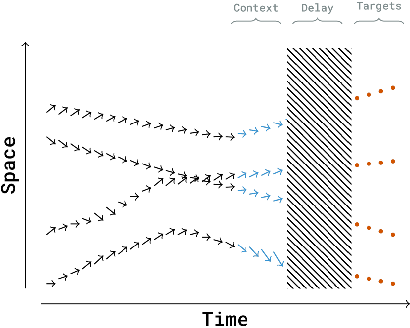
(a) Description of the context and target sets in the wind nowcasting case. The context set and the target set are time slices separated by a delay, which corresponds to the forecasting window. The underlying space is in that case $\mathbb{X}\subseteq\mathbb{R}^{3}$ and the context values and target values both are representing wind speed and belong to the same space $\mathbb{I}=\mathbb{O}\subseteq\mathbb{R}^{2}$.

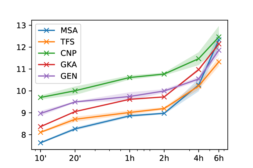
(b) RMSE of the different models depending on the forecast duration (lower is better). We ran three experiments varying the pseudorandom number generator seeds for each time window and each model to measure the standard deviation. The error is not increasing drastically over the first two hours because the wind has some persistence and the context values are good predictors of the targets in that regime.

Table 1: Validation RMSE of the High-Altitude Wind Nowcasting, Poisson, Navier Stokes and Darcy Flow equation and the weather forecasting task. Each model ran for respectively 10, 2000, 1000, 100 and 100 epochs on an NVIDIA GeForce GTX 1080 Ti. The low number of epochs for wind nowcasting is due to the amount of data which is considerably larger than in the other experiments. The standard deviation is computed over 3 runs. We present here the original implementation of CNP and GEN compared with TFS and MSA with sharing weights for the position. More details can be found in  section 7 of the supplementary material. We choose the configuration of the models so that every model has a comparable number of parameters. We underline the best models for each size and indicate in bold the best model overall.

Model	Size	Wind Nowcasting	Poisson Equation	Navier Stokes Equation	Darcy Flow Equation	ERA5
CNP	5k	11.94$\pm$ 0.78	0.33$\pm$ 0.004	0.701$\pm$ 0.0023	0.0311$\pm$ 0.0008	2.129$\pm$ 0.0039
	20k	10.19$\pm$ 1.83	0.32$\pm$ 0.003	0.672$\pm$ 0.0011	0.0295$\pm$ 0.0002	2.117$\pm$ 0.0018
	100k	10.17$\pm$ 1.24	0.33$\pm$ 0.003	0.656$\pm$ 0.0007	0.0286$\pm$ 0.0001	2.110$\pm$ 0.0002
GEN	5k	11.02$\pm$ 3.19	0.12$\pm$ 0.006	0.604$\pm$ 0.0010	0.0304$\pm$ 0.0003	2.132$\pm$ 0.0035
	20k	9.98$\pm$ 0.76	0.13$\pm$ 0.014	0.599$\pm$ 0.0006	0.0296$\pm$ 0.0002	2.124$\pm$ 0.0031
	100k	9.56$\pm$ 0.21	0.16$\pm$ 0.049	0.596$\pm$ 0.0005	0.0294$\pm$ 0.0001	2.121$\pm$ 0.0005
TFS (Ours)	5k	8.30$\pm$ 0.03	0.15$\pm$ 0.036	0.604$\pm$ 0.0022	0.0275$\pm$ 0.0014	2.129$\pm$ 0.0032
	20k	8.20$\pm$ 0.04	0.09$\pm$ 0.006	0.596$\pm$ 0.0008	0.0258$\pm$ 0.0003	2.109$\pm$ 0.0012
	100k	8.38$\pm$ 0.13	0.18$\pm$ 0.014	0.591$\pm$ 0.0012	0.0269$\pm$ 0.0004	2.100$\pm$ 0.0011
MSA (Ours)	5k	8.07$\pm$ 0.11	0.11$\pm$ 0.006	0.597$\pm$ 0.0011	0.0274$\pm$ 0.0011	2.125$\pm$ 0.0070
	20k	7.98$\pm$ 0.03	0.08$\pm$ 0.003	0.589$\pm$ 0.0013	0.0259$\pm$ 0.0007	2.107$\pm$ 0.0020
	100k	8.18$\pm$ 0.14	0.10$\pm$ 0.009	0.589$\pm$ 0.0006	0.0264$\pm$ 0.0004	2.098$\pm$ 0.0029

Table 2: Evaluation of the wind nowcasting task according to standard weather metrics, which are described in section 11 of the supplementary material. The optimal value of the metric is indicated in the parenthesis. MSA is the best model overall, with the lowest absolute error, a near zero systematical bias and output values that have a similar dispersion to GEN.

Model	RMSE ($\downarrow$)	$\theta$ MAE ($\downarrow$)	$r$ MAE ($\downarrow$)	Relative $\text{BIAS}_{x}$ (0.0)	Relative $\text{BIAS}_{y}$ (0.0)	rSTD (1.0)	NSE ($\uparrow$)
CNP	10.99$\pm$ 0.75	25.55$\pm$ 1.22	9.22$\pm$ 0.33	0.00$\pm$ 0.09	-1.09$\pm$ 0.03	1.25$\pm$ 0.07	-0.23$\pm$ 0.01
GEN	8.97$\pm$ 0.06	22.56$\pm$ 0.77	6.97$\pm$ 0.05	-0.02$\pm$ 0.03	-0.97$\pm$ 0.21	1.09$\pm$ 0.07	0.25$\pm$ 0.02
GKA	8.44$\pm$ 0.01	21.89$\pm$ 0.02	6.65$\pm$ 0.02	-0.02$\pm$ 0.00	-1.78$\pm$ 0.02	1.13$\pm$ 0.00	0.31$\pm$ 0.01
TFS (Ours)	7.99$\pm$ 0.15	22.17$\pm$ 1.20	6.48$\pm$ 0.50	0.08$\pm$ 0.10	-2.21$\pm$ 2.67	1.17$\pm$ 0.04	0.43$\pm$ 0.08
MSA (Ours)	7.36$\pm$ 0.06	20.48$\pm$ 0.48	5.67$\pm$ 0.11	0.00$\pm$ 0.02	-0.04$\pm$ 0.64	1.09$\pm$ 0.02	0.55$\pm$ 0.05

Our experiments aim to benchmark the performance of our models on various irregularly sampled datasets. The first task focuses on high-altitude wind nowcasting. The second task is on heat diffusion. Additionally, we evaluate our models on fluid flows, considering both a steady-state case governed by the Darcy Flow equation and a dynamic case modeling the Navier-Stokes equation in an irregularly spaced setting. Finally, we compare the models on a weather forecasting task, utilizing irregularly sampled measurements from the ERA5 dataset [11] to predict wind conditions two days ahead.

For the Wind Nowcasting Experiment, the dataset, described in section 3.1, consists of wind speed measurements collected by airplanes with a sampling frequency of four seconds. We evaluated our models on this dataset [table 1] and we assess the models’ performance as a function of forecast duration, as depicted in fig. 2(b). We select model configurations with approximately 100,000 parameters and ran each model using three different random seeds. Our results indicate that attention-based models consistently outperformed other models for most forecast durations, except for in the 6-hour range. Notably, we found that the GKA model used in previous work achieved satisfactory performance, despite its theoretical limitations. A detailed comparison with the GKA model can be found in section 10 of the supplementary material. Moreover, our findings suggest that attention-based models, particularly MSA and TFS, exhibited superior performance in this setup. Furthermore, we observed that the GKA model performed well for short time horizons when most of the information in the context was still up-to-date. However, as the time horizon increased, the GKA model’s lack of flexibility became more apparent, and GEN became more competitive.

For the Heat Diffusion Experiment, we utilize the dataset introduced in [1], derived from a Poisson Equation solver. The dataset consists of context measurements in the unit square corresponding to sink or source points, as well as points on the boundaries. The targets correspond to irregularly sampled heat measurements in the unit cube. Our approach demonstrated significant performance improvements, reducing the root mean square error (RMSE) from 0.12 to 0.08, (MSE reduction of 0.016 to 0.007, in term of the original metric) as measured against the ground truth [table 1].

For the Fluid Flow Experiment, both datasets are derived from [18], subsampled irregularly in space. In both cases, our models outperformed the alternative [table 1]. In the Darcy Flow equation, the TFS model with 20k parameters exhibited the best performance, but this task proved to be relatively easier, and we hypothesize that the MSA model could not fully exploit this specific setup. However, it is worth mentioning that the performance of the MSA model was within a standard deviation of the TFS model.

We conducted a Two-Day Weather Forecasting Experiment utilizing ERA5 dataset measurements. The dataset consists of irregularly sampled measurements of seven quantities, including wind speed at different altitudes, heat, and cloud cover. Our goal is to predict wind conditions at 100 meters two days ahead based on these measurements. MSA demonstrates its effectiveness in capturing the temporal and spatial patterns of weather conditions, enabling accurate predictions [table 1].

To summarize, our experiments encompass a range of tasks including high-altitude wind nowcasting, heat diffusion, fluid modeling, and two-day weather forecasting. Across these diverse tasks and datasets, our proposed model consistently outperforms baseline models, showcasing their efficacy in capturing complex temporal and spatial patterns.

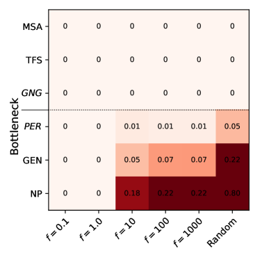
Figure 3: Results of the information retrieval experiment. The three first rows correspond to models with no bottlenecks. The x-axis corresponds to datasets created by increasing frequency. When the learned function does not vary too much spatially, models with bottlenecks can suffice. GEN uses a $7\times 7$ grid initialization. The models in italics represent hybrid architectures: GNG = GEN without a graph, which maintains a latent per context measure and PER = transformer with a perceiver layer [12] which creates a bottleneck.

5 Understanding failure modes

We examine the limitations of CNP and GEN latent representation for encoding a context. Specifically, we focus on the bottleneck effect that arises in CNP from using a single vector to encode the entire context, resulting in an underfitting problem [7, 14], and that applies similarly to GEN. To highlight this issue, we propose three simple experiments. (1) We show in which case baselines are not able to retrieve information in the context that they use for conditioning, and why MSA and TFS are not suffering from this problem. (2) We show that maintaining disentangled latent representation helped to the correct attribution of perturbations. (3) We show that this improved latent representation leads to better error correction.

5.1 Context information retrieval

Every model considered in this work encodes context information differently. Ideally, each should be capable of using or retrieving every measure in their context. We will see that excessive bottlenecking in the latent space can make this difficult or impossible.

To demonstrate this result, we design a simple experiment in which each model encodes a set of 64 measures $(\mathbf{c}_{x},\mathbf{c}_{y})$, and is then tasked with retrieving the corresponding $\mathbf{t}_{y}=\mathbf{c}_{y}$ given the $\mathbf{t}_{x}=\mathbf{c}_{x}$. The training and validation set have respectively $10,000$ and $1,000$ pairs of sets of $64$ examples. It is worth noting that the models have access to all the information they need to solve the task with near-zero MSE. We conducted several experiments, starting by randomly sampling 2D context positions $\mathbf{c}_{x}=(x,y)$ from a Gaussian distribution and computing the associated deterministic smooth function:

$$\mathbf{c}_{y}=\sin(\pi fx)\cos(\pi fy)\in\mathbb{R}$$ (1)

where $f$ is a frequency parameter that governs problem difficulty. The higher $f$ is, the more difficult the function becomes, as local information becomes less informative about the output.

The results of this experiment, presented in fig. 3, show that CNP and GEN fail to effectively learn this task when the frequency is too high. This occurs when a single latent variable is supposed to represent two different context measurements, and prevents the models from retrieving the correct target value. In contrast, models with disentangled latent representations, such as MSA, can effectively learn the task.

To further demonstrate this bottleneck effect, we created two hybrid models. The first one denoted GNG (for GEN No Graph), is adapted from GEN but instead of relying on a common graph, creates one based on the measure position with one node per measure. Edges are artificially added between neighboring measures which serve as the base structure for $L$ steps of message-passing. This latent representation is computationally expensive as it requires the creation of a graph per set of measurements, but it does not create a bottleneck in the latent representation. We found that GNG is indeed able to learn the task at hand. We then followed the reverse approach and artificially added a bottleneck in the latent representation of attention-based models by using Perceiver Layer  [12] with $P$ learned latent vectors instead of the standard self-attention in the transformer encoder (and call the resultant model PER). When $P$ is smaller than the number of context measurements, it creates a bottleneck and PER does not succeed in learning the task. If the underlying space is smooth enough, GEN, CNP and PER are capable of reaching perfect accuracy on this task as they can rely on neighboring values to retrieve the correct information. This experiment demonstrates that MSA and TFS can use their disentangled latent representations to efficiently retrieve context information regardless of the level of discontinuity in the underlying space, while models with bottlenecks, such as CNP and GEN, are limited in this regard and perform better when the underlying space is smooth.

5.2 Correct pertubation attribution

In the following analysis, we explore how disentangled latent representations can enhance error correction during training. Specifically, we ask whether models can correctly attribute the effects of a perturbation in the output to backpropagation.

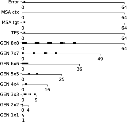
Figure 4: Gradients on the last layer of the encoder corresponding to an artificial error of $\gamma=10.0$ added to the second output. MSA maintains a disentangled representation and the gradient at that layer is non-zero only on the corresponding latent. We compare it to different GEN models each initialized with a graph corresponding to a regular grid of size $i\times i$ with $i\in\{1,\dots,8\}$. Due to the bottleneck effect, the gradients corresponding to one error are propagated across different latent vectors for GEN. Even when there are enough latents (GEN 8 $\times$ 8), GEN still disperse attribution because their distance-based conditioning that does not allow for a one-to-one mapping between targets and latents.

We use MSA, TFS and GEN models applied to the information retrieval task discussed in the previous section. We pre-train each model to zero error on the validation data in a smooth case ($f=1.0$) and then apply a perturbation $\gamma$ on one of the output values, compute the loss between the perturbated output and the one without perturbation and backpropagate it through each model. The norm of gradients corresponding to the latent at the last encoder layer is shown in  fig. 4. We see that MSA and TFS only receive a signal on the corresponding latent while the other models receive signals on different latents. Here MSA has $128$ latent vectors as it maintains one latent per context measurement and per target position, and we see that the model has a signal only on the latent corresponding to the position where there is an error.

We hypothesize that this interference of gradients to other non-related latents impedes training, as the models struggle to correct the artificial error while maintaining the same value for the other output values. Models with a disentangled representation can update the corresponding latent independently and follow a smoother optimization trajectory.

To demonstrate this property, for the models described above, we tabulate the number of backpropagation passes needed to fully correct the artificial error on one output (to reach a zero error on the validation set again).

The results are shown in fig. 5. We used MSA as a reference and observed that all models with an entangled representation required more time to reach a zero error on the validation set. We found that the more entangled the representation, the more time was needed to reach the desired performance. Note that, in this setup, GEN 1 $\times$ 1 is equivalent to CNP.

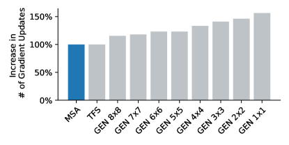
Figure 5: Comparison of the number of gradient updates required to correct an artificial error, with respect to MSA (lower is better). The y-axis represents the increase in percentage in the number of steps required to reach a perfect accuracy with respect to MSA. We compared MSA to different GEN each initialized with a graph corresponding to a regular grid of size $i\times i$ with $i\in\{1,\dots,8\}$. It can be observed that all GEN take more steps to correct the same mistake, and the more entangled the latent representation is, the more time it requires to correct the problem.

These experiments demonstrate that models with disentangled latent representations can more efficiently correct errors during training, while models with entangled representations struggle to do so and require more time to reach the desired performance.

5.3 Encoding scheme

We propose in this section a novel encoding scheme for this task of forecasting conditioned on a context. Our approach leverages the fact that both the context measurements and target positions reside within a shared underlying space. To exploit this shared structure, we adopt a unified MLP encoder for mapping both the context and target position to a latent space representation. This differs from the approach proposed in Garnelo et al. [7], Alet et al. [1] where the unprocessed target position is concatenated to a single latent or a weighted average of the neighboring latent vectors. The main technical challenge with this approach lies in encoding the associated values of the context value, while ensuring that the resulting vector has the same dimension for processing by the attention model. To address this, we use a second MLP to encode the context values and add them with their corresponding encoded positions.

Mathematically this can be written as:

$$c_{e} =\text{MLP}_{p}(\mathbf{c}_{x})+\text{MLP}_{v}(\mathbf{c}_{y})$$

$$t_{e} =\text{MLP}_{p}(\mathbf{t}_{x})$$

Where $c_{e}$ and $t_{e}$ correspond to the encoded context and target input respectively, and $\text{MLP}_{p}$ and $\text{MLP}_{v}$ are both multi-layer perceptrons. In section 7 of the supplementary material, we observe that this scheme improves the performance of most models. Notably, it reduces the RMSE from 8.47 to 7.98 in the wind nowcasting task and enables the MSA model to achieve the best performance with an RMSE of 0.08 for the Poisson Equation. Sharing the same mapping for positions is the appropriate inductive bias for encoding positions, as it eliminates the need to learn the same transformation twice. Since our data is irregularly sampled in space, the positioning of measurements and target positions significantly influences the prediction, as demonstrated in additional experiments (see sections 12 and 13 in the supplementary material). We think that sharing the position mapping can link information from the context and target positions, which helps the model to understand better how the space is shaped.

6 Conclusion

In this work, we introduced an attention-based model to handle the challenges of wind nowcasting data. We demonstrated that the proposed attention-based model was able to reach the best performance for high-altitude wind prediction and other dynamical systems, such as weather forecasting, heat diffusion and fluid dynamics when working with data irregularly sampled in space. We then explained why attention-based models were capable of outperforming other models on that task and provided an in-depth examination of the differences between models, providing explanations for the impact of design choices such as latent representation bottlenecks on the final performance of the trained models.

As part of our future work, we intend to extend our attention-based model by incorporating additional information sources, such as topography and other weather covariates in a wind forecasting problem. With proper methodological enhancement models across domains can achieve more accurate and reliable predictions by incorporating auxiliary information.

7 Detailed results

Here, we present a breakdown of the detailed results for the various models, presented in terms of the specific metrics reported in their original study. This is in contrast to the result table found in the main paper, where all models are reported in terms of RMSE. In table 1, we provide the results for GEN and CNP based on their original implementations, which do not involve sharing the position encoding. However, for TFS and MSA, we include the results obtained with shared position encoding. To ensure comprehensiveness and to differentiate the enhanced performance attributed to the latent representation from that resulting from the improved data encoding approach, we also apply the shared encoding technique to GEN and CNP.

In most cases, we observe that employing a shared encoding for position tends to improve the performance of all models, except for CNP where it seems to decrease the overall performance in some cases. Additionally, it seems that MSA surpasses its competitors in the majority of instances, consistently exhibiting superior performance across various data sizes. Moreover, when the shared encoding for positions fails to achieve the optimal performance, the model’s performance is generally comparable to that without shared encoding, often falling within a standard deviation range.

Table 1-2: Results of the High-Altitude Wind Nowcasting, Poisson, Navier Stokes and Darcy Flow equation and the weather forecasting task. Each model ran for respectively 10, 2000, 1000, 100, and 100 epochs on an NVIDIA GeForce GTX 1080 Ti. The low number of epochs for wind nowcasting is due to the amount of data which is considerably larger than in the other experiments. The standard deviation is computed over 3 runs. We choose the configuration of the models so that every model has a comparable number of parameters. We underlying the best models for each size and we put in bold the best model overall. In this table, we kept the results in the same metric as originally reported. The first half of the table corresponds to the case without the novel encoding scheme, as opposed to the second one. In table 1, we recomputed all metrics in terms of Root Mean Square Error (RMSE).

		Wind Nowcasting		Poisson Equation		Navier Stokes Equation		Darcy Flow Equation		ERA 5
Model	Size	Train RMSE ($\downarrow$)	Val RMSE ($\downarrow$)	Train MSE ($\downarrow$)	Val MSE ($\downarrow$)	Train MSE ($\downarrow$)	Val MSE ($\downarrow$)	Train RMSE ($\downarrow$) E-4	Val RMSE ($\downarrow$)	Train MSE ($\downarrow$)	Val MSE ($\downarrow$)
Default encoding for positions
CNP	5k	11.94$\pm$ 0.78	10.19$\pm$ 0.21	.127$\pm$ .0179	.130$\pm$ .0134	.485$\pm$ .0033	.492$\pm$ .0033	9.02$\pm$ 0.54	9.65$\pm$ 0.47	4.33$\pm$ 0.01	4.48$\pm$ 0.01
	20k	10.19$\pm$ 1.83	10.11$\pm$ 0.20	.084$\pm$ .0057	.105$\pm$ .0012	.438$\pm$ .0015	.452$\pm$ .0015	7.88$\pm$ 0.16	8.71$\pm$ 0.11	4.25$\pm$ 0.01	4.44$\pm$ 0.00
	100k	10.17$\pm$ 1.24	10.20$\pm$ 0.26	.021$\pm$ .0040	.105$\pm$ .0024	.398$\pm$ .0010	.430$\pm$ .0010	6.93$\pm$ 0.08	8.17$\pm$ 0.06	4.17$\pm$ 0.01	4.43$\pm$ 0.01
GEN	5k	11.02$\pm$ 3.19	9.84$\pm$ 2.92	.011$\pm$ .0006	.017$\pm$ .0011	.362$\pm$ .0012	.365$\pm$ .0012	8.49$\pm$ 0.17	9.25$\pm$ 0.18	4.32$\pm$ 0.02	4.47$\pm$ 0.02
	20k	9.98$\pm$ 0.76	9.24$\pm$ 0.35	.006$\pm$ .0006	.020$\pm$ .0054	.354$\pm$ .0007	.359$\pm$ .0007	7.76$\pm$ 0.11	8.74$\pm$ 0.09	4.24$\pm$ 0.01	4.44$\pm$ 0.00
	100k	9.56$\pm$ 0.21	9.23$\pm$ 0.44	.011$\pm$ .0122	.048$\pm$ .0389	.339$\pm$ .0006	.355$\pm$ .0006	7.01$\pm$ 0.26	8.66$\pm$ 0.09	4.10$\pm$ 0.01	4.46$\pm$ 0.00
TFS (Ours)	5k	9.86$\pm$ 0.21	8.75$\pm$ 0.14	.022$\pm$ .0021	.055$\pm$ .0248	.365$\pm$ .0033	.367$\pm$ .0033	6.50$\pm$ 0.60	7.46$\pm$ 0.55	4.29$\pm$ 0.02	4.46$\pm$ 0.00
	20k	9.69$\pm$ 0.38	8.70$\pm$ 0.06	.005$\pm$ .0008	.017$\pm$ .0014	.353$\pm$ .0019	.357$\pm$ .0019	5.48$\pm$ 0.10	6.69$\pm$ 0.14	4.08$\pm$ 0.03	4.38$\pm$ 0.01
	100k	9.55$\pm$ 0.19	8.67$\pm$ 0.07	.001$\pm$ .0001	.016$\pm$ .0045	.314$\pm$ .0011	.350$\pm$ .0011	4.45$\pm$ 0.17	7.47$\pm$ 0.24	3.78$\pm$ 0.01	4.42$\pm$ 0.01
GPT (Ours)	5k	8.86$\pm$ 0.01	8.40$\pm$ 0.10	.022$\pm$ .0062	.048$\pm$ .0186	.359$\pm$ .0057	.361$\pm$ .0054	6.91$\pm$ 0.50	7.74$\pm$ 0.48	4.28$\pm$ 0.02	4.44$\pm$ 0.02
	20k	7.94$\pm$ 0.03	8.47$\pm$ 0.12	.005$\pm$ .0012	.047$\pm$ .0107	.341$\pm$ .0042	.346$\pm$ .0042	5.72$\pm$ 0.11	6.76$\pm$ 0.10	4.13$\pm$ 0.01	4.39$\pm$ 0.01
	100k	6.67$\pm$ 0.02	8.98$\pm$ 0.22	.000$\pm$ .0001	.030$\pm$ .0081	.310$\pm$ .0015	.350$\pm$ .0015	4.91$\pm$ 0.17	7.33$\pm$ 0.22	4.19$\pm$ 0.01	4.41$\pm$ 0.01
Sharing encoding for positions
CNP	5k	10.41$\pm$ 0.03	10.33$\pm$ 0.19	.154$\pm$ .0010	.165$\pm$ .0023	.703$\pm$ .0001	.706$\pm$ 0.0003	16.94$\pm$ 0.06	17.26$\pm$ 0.04	4.38$\pm$ 0.00	4.53$\pm$ 0.01
	20k	9.48$\pm$ 0.02	10.12$\pm$ 0.21	.133$\pm$ .0004	.160$\pm$ .0011	.700$\pm$ .0001	.706$\pm$ 0.0001	16.68$\pm$ 0.10	17.06$\pm$ 0.06	4.30$\pm$ 0.01	4.47$\pm$ 0.00
	100k	8.60$\pm$ 0.05	10.26$\pm$ 0.24	.107$\pm$ .0008	.158$\pm$ .0006	.696$\pm$ .0001	.705$\pm$ 0.0001	16.36$\pm$ 0.02	16.87$\pm$ 0.02	4.23$\pm$ 0.01	4.43$\pm$ 0.01
GEN	5k	10.04$\pm$ 0.13	8.79$\pm$ 0.23	.005$\pm$ .0004	.017$\pm$ .0023	.369$\pm$ .0007	.372$\pm$ 0.0008	5.93$\pm$ 0.15	6.83$\pm$ 0.17	4.42$\pm$ 0.01	4.54$\pm$ 0.01
	20k	9.75$\pm$ 0.09	9.08$\pm$ 0.47	.003$\pm$ .0007	.018$\pm$ .0036	.362$\pm$ .0002	.366$\pm$ 0.0000	5.65$\pm$ 0.06	6.75$\pm$ 0.05	4.36$\pm$ 0.01	4.50$\pm$ 0.01
	100k	9.84$\pm$ 0.02	9.07$\pm$ 0.00	.001$\pm$ .0000	.019$\pm$ .0008	.345$\pm$ .0005	.361$\pm$ 0.0000	4.97$\pm$ 0.22	7.19$\pm$ 0.12	4.34$\pm$ 0.02	4.50$\pm$ 0.01
TFS (Ours)	5k	8.78$\pm$ 0.02	8.30$\pm$ 0.03	.009$\pm$ .0015	.025$\pm$ .0121	.364$\pm$ .0024	.365$\pm$ 0.0026	6.74$\pm$ 0.93	7.58$\pm$ 0.84	4.41$\pm$ 0.01	4.53$\pm$ 0.01
	20k	7.94$\pm$ 0.03	8.20$\pm$ 0.04	.002$\pm$ .0002	.010$\pm$ .0013	.352$\pm$ .0012	.355$\pm$ 0.0009	5.56$\pm$ 0.10	6.64$\pm$ 0.14	4.26$\pm$ 0.01	4.45$\pm$ 0.01
	100k	6.57$\pm$ 0.02	8.38$\pm$ 0.13	.000$\pm$ .0000	.035$\pm$ .0054	.312$\pm$ .0006	.349$\pm$ 0.0015	4.51$\pm$ 0.24	7.25$\pm$ 0.19	4.09$\pm$ 0.01	4.41$\pm$ 0.00
GPT (Ours)	5k	8.54$\pm$ 0.03	8.07$\pm$ 0.11	.008$\pm$ .0024	.014$\pm$ .0014	.355$\pm$ .0013	.357$\pm$ 0.0013	6.74$\pm$ 0.61	7.51$\pm$ 0.61	4.38$\pm$ 0.03	4.52$\pm$ 0.03
	20k	7.73$\pm$ 0.02	7.98$\pm$ 0.03	.002$\pm$ .0003	.007$\pm$ .0004	.342$\pm$ .0014	.347$\pm$ 0.0016	5.79$\pm$ 0.34	6.74$\pm$ 0.38	4.25$\pm$ 0.01	4.44$\pm$ 0.01
	100k	6.58$\pm$ 0.05	8.18$\pm$ 0.14	.000$\pm$ .0000	.010$\pm$ .0017	.310$\pm$ .0008	.347$\pm$ 0.0008	4.76$\pm$ 0.12	6.97$\pm$ 0.24	4.14$\pm$ 0.02	4.40$\pm$ 0.01

8 Dataset descriptions

8.1 Wind nowcasting

The wind nowcasting experiment uses the same dataset as Pannatier et al. [20]. It is available at: https://zenodo.org/record/5074237. It is an important task for ATC as it involves the crucial prediction of high-altitude winds using real-time data transmitted by airplanes. This prediction is essential for ensuring efficient airspace management the airspace. Notably, when considering the vertical direction ($z$), a majority of wind measurements are obtained at elevated altitudes ranging from 4,000 to 12,000 meters. As ground-based measurements are not accessible at these heights, our dependence lies on the measurements gathered directly from airplanes. As planes do not record the wind in the $z$ direction, the input space corresponds to wind speed in the $x,y$ plane $\mathbb{I}\subseteq\mathbb{R}^{2}$, and the output space is the wind speed measured later, $\mathbb{O}\subseteq\mathbb{R}^{2}$. Here the underlying space is European airspace represented as $\mathbb{X}\subseteq\mathbb{R}^{3}$ In this particular setup, the models need to extrapolate in time, based on a set of the last measurements.

Airplanes measure wind speed with a sampling frequency of four seconds. We split the dataset into time slices, where each slice contains one minute of data, such that each time slice contains between 50 and 1500 data points. We tried different time intervals but noticed that having a longer time slice did not improve the quality of the forecasts. The objective for the different models is to output a prediction of the wind at different query points 30 minutes later. We evaluate performance using the Root Mean Square Error (RMSE) metric, as in previous work.

8.2 Poisson Equation

This experiment uses the same dataset as [1]. It is available at https://github.com/FerranAlet/graph_element_networks/tree/master/data. The Poisson equation models the heat diffusions over the unit square with sources represented by $\phi(x,y)\in\mathbb{R}$ and fixed boundary conditions $\omega\in\mathbb{R}$. The equation is given by:

$$\begin{cases}\Delta\phi(x,y)=\psi(x,y)&\text{if}\ (x,y)\in(0,1)^{2}\\ \phi(x,y)=\omega&\text{if}\ (x,y)\in\partial[0,1]^{2}\end{cases}$$ (2)

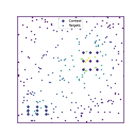
Figure 6: A sample of the Poisson equation dataset [1]. $\bullet$ represents the targets, The context values are comprised of points on the boundaries and points on the sources and sink are represented by $\blacklozenge$ which corresponds to their thermal coefficient.

It should be noted that the boundary constant and sources function $\phi(x,y)$ conditions can change for each sample.

The dataset used in [1] uses three dimensions for the context values $\mathbf{c}_{y}\in\mathbb{I}\subseteq\mathbb{R}^{3}$: either sources values $\phi(x,y)=\mu$ inside the domain encoded as $\mathbf{c}_{x},\mathbf{c}_{y}=(x,y),(\mu,0,0)$ or boundary conditions $\phi(x,y)=\omega$ on the boundaries, encoded as $\mathbf{c}_{x},\mathbf{c}_{y}=(x,y),(0,\omega,1)$. The target space is one-dimensional $\mathbf{t}_{y}\in\mathbb{O}\subseteq\mathbb{R}$ and corresponds to the solution of the Poisson equation at that point. A sample is depicted in fig. 6.

We ran all models for three different sizes on this particular setup and found that MSA with the novel encoding scheme outperform other models by a significant margin as can be seen in section 7. We initialized GEN with a $7\times 7$ regularly initialized grid on the $[0,1]^{2}$ as in the original work [1].

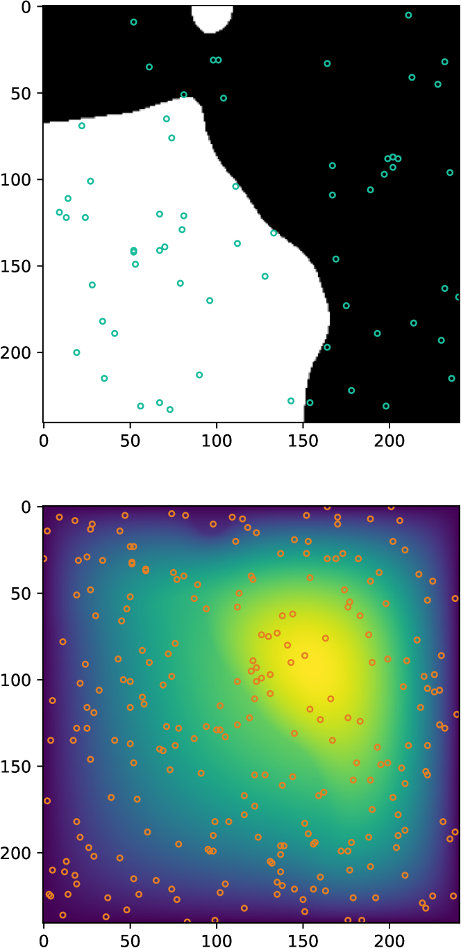
(a) A sample of the Darcy Flow dataset [18]. Blue dots correspond to the context set and orange dots to the targets.

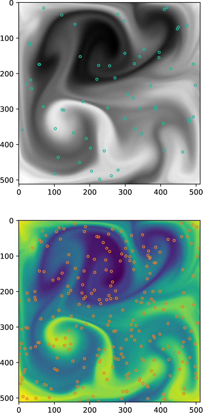
(b) A sample of the Navier-Stokes dataset [18]. Blue dots correspond to the context set and orange dots to the targets.

8.3 Navier-Stokes Equation

Similarly to the darcy flow task, we adapted the Navier-Stokes equation as described in [18] to an irregular setup.

The Navier-Stokes equation describes a real fluid and is described with the following PDE :

$$\begin{cases}\partial_{t}w(x,t)+u(x,t)\cdot\nabla w(x,t)=\nu\Delta w(x,t)+f(x),x\in(0,1)^{2}&\text{if}\ t\in(0,T]\\ \nabla\cdot u(x,t)=0,x\in(0,1)^{2}&\text{if}\ t\in[0,T]\\ w(x,0)=w_{0}(x)&\text{if}\ x\in(0,1)^{2}\end{cases}$$ (3)

For more detailed information regarding the notation, please refer to the original work by Li et al. [18], specifically section 5.3.

In this study, our objective is to forecast the future state of the vorticity quantity, specifically 50 time steps ahead, based on measurements of vorticity at different spatial locations. This approach differs from the original work, where the model was provided with ten initial vorticity grids and required to predict the complete system evolution.

To create our dataset, we subsampled the complete dataset, which consisted of the evolution of the Navier-Stokes equation solved by a numerical solver. The full dataset had dimensions of $1000\times 1024\times 1024$.

For our purposes, we selected pairs of slices that were separated by 50 timesteps and performed spatial subsampling. We took 64 context measurements and 256 targets as our subsampled data points. This experiment adapts the dataset available in [18]. It is available at https://github.com/neural-operator/fourier_neural_operator and can be processed with the code given to rearrange it in the irregular setup.

8.4 Darcy Flow

We evaluated the performance of various models in solving the Darcy Flow equation on the unit grid with null boundary conditions, as described in [18]. Specifically, we aimed to predict the value of the function $u$, given the diffusion function $a$, with the two related implicitly through the PDE given by:

$$\begin{cases}-\nabla\cdot(a(x)\nabla u(x))=1&\textnormal{ if }x\in(0,1)^{2}\\ u(x)=0&\textnormal{ if }x\in\partial[0,1]^{2}.\end{cases}$$ (4)

The dataset used in our study is adapted from that used in [18], and originally generated by a traditional high-resolution PDE solver. The dataset consists of a 1024 $\times$ 1024 grid, which was subsampled uniformly at random and arranged into context-target pairs. The context is comprised of the evaluations of the diffusion coefficient: $(\mathbf{c}_{x},\mathbf{c}_{y})=((x,y),a(x,y))$, and the target is the solution of the Darcy Flow equation at a position, $(\mathbf{t}_{x},\mathbf{t}_{y})=((x,y),u(x,y))$.

The results are presented in section 7, they are coherent with the rest of the experiment and show that the MSA and TFS models are able to outperform all competing models. We used the same initialization for GEN as for the Poisson Equation.

This experiment adapts the dataset available in [18]. It is available at https://github.com/neural-operator/fourier_neural_operator and can be processed with the code provided to rearrange it in the irregular setup.

8.5 Two-Days Weather Forecasting

In this task, we want to evaluate our models on the task of two-days weather forecasting based on irregularly sampled data in space. The requested data collection description focuses on climate reanalysis from the ERA5 dataset, which is available through the Copernicus Climate Data Store (CDS). The dataset contains various parameters related to wind, surface pressure, temperature, and cloud cover.

To access the data, please visit the following URL: https://cds.climate.copernicus.eu/cdsapp#!/dataset/reanalysis-era5-single-levels?tab=form.

We selected the following variables:

• 10m u-component of wind: This refers to the eastward wind component at a height of 10 meters above the surface.

• 10m v-component of wind: This represents the northward wind component at a height of 10 meters above the surface.

• 100m u-component of wind: This denotes the eastward wind component at a height of 100 meters above the surface.

• 100m v-component of wind: This signifies the northward wind component at a height of 100 meters above the surface.

• Surface pressure: This represents the atmospheric pressure at the Earth’s surface.

• 2m temperature: This indicates the air temperature at a height of 2 meters above the surface.

• Total cloud cover: This refers to the fraction of the sky covered by clouds. The data collection includes measurements for all times of the day and all days available in the dataset. However, for training purposes, we selected the data from the year 2000. For validation, we use the data from the year 2010, specifically the months of January and September.

Next, we proceeded to extract the corresponding grib files. To create our dataset, we paired time slices that had a time difference of two days, equivalent to 48 time steps since ERA5 data has a one-hour resolution.

For the context slice, we performed subsampling at 1024 different positions and retained all seven variables mentioned earlier. As for the target slice, we subsampled it at 1024 different positions and kept only the two components of the wind at 100m.

Dataset	$\dim(\mathbb{X})$	$\dim(\mathbb{I})$	$\dim(\mathbb{O})$	# Train. points	# Val. points	URL
Wind Nowcasting	3	2	2	26.956.857	927.906	[20] Dataset page
Poisson Equation	2	3	1	409.600	102.400	[1] Github Repository
Navier Stokes Equation	2	1	1	48.883.20	11.673.600	[18] Github Repository
Darcy Flow Equation	2	1	1	409.600	102.400	[18] Github Repository
ERA5	2	7	2	8.648.704	2.107.392	[11] Copernicus Climate Dataset Store
Random	2	1	1	640.000	64.000	Randomly generated
Sine	2	1	1	640.000	64.000	Randomly generated

Table 3: Description of the different datasets used in this study.

9 Attention matrix for Wind Nowcasting

For all models, we can plot the norm of the input gradients to see how changing a given value would impact the prediction [fig. 8]. We see that Transformers seem to find a trade-off between taking into account the neighboring nodes and the global context.

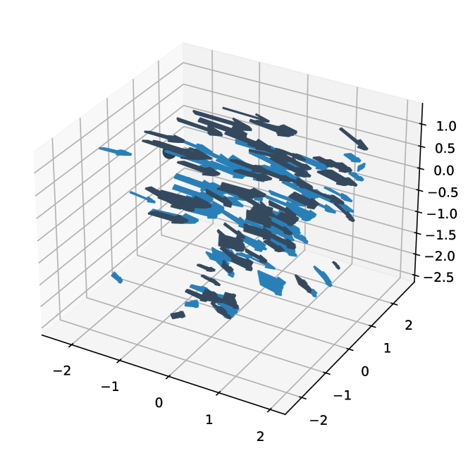
(a) Context, Targets

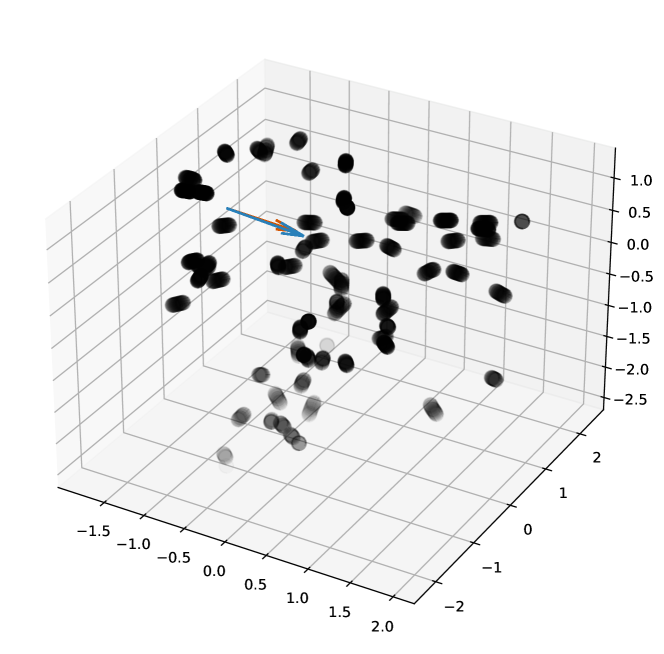
(b) MSA (Ours)

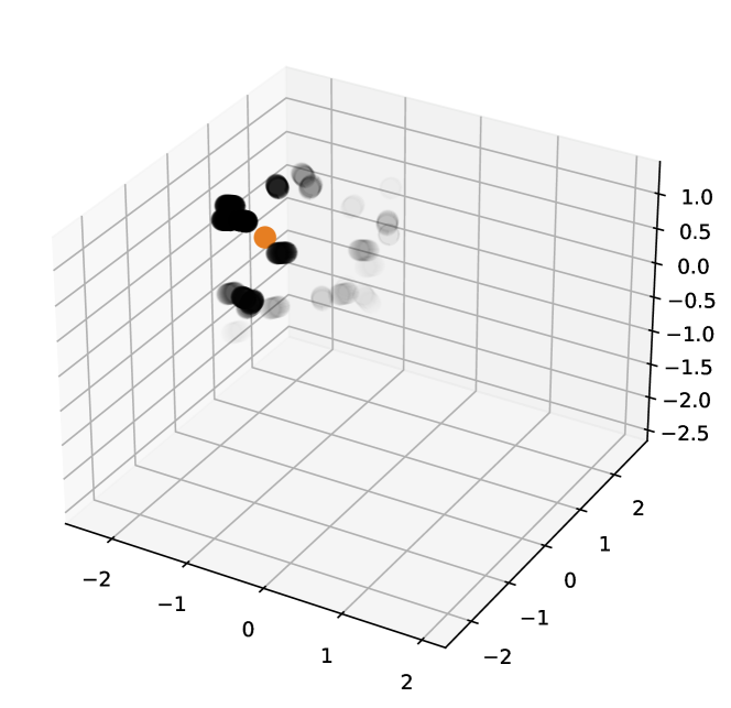
(c) GKA [20]

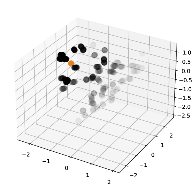
(d) GEN [1]

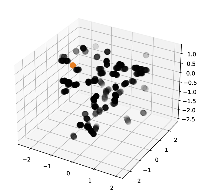
(e) CNP [7]

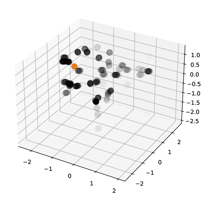
(f) TFS (Ours)

Figure 8: Displaying the importance given to points in the context to do the prediction for the different models for a given query point (orange). We used the norm of the input gradients for that purpose and highlight the context values that have the largest gradient with respect to the output. The opacity of the dots corresponds to the relative magnitude of the input gradients compared to other points in the context.

10 Comparison with Graph Kernel Averaging

Smart averaging strategies such as GKA are limited by design to the range of the values in their context. However, these baselines are useful as they are not prone to overfitting and in the case of time series forecasting (if the underlying variable has some persistence), the last values would in general be the best predictor of the next value. We hypothesize that over sufficiently short horizons, these methods would achieve performance similar to that from more complicated models, but when the prediction horizon rises, this design limitation would become more pronounced.

Since, for extrinsic forecasting, target points need not lie in the convex hull of context points, the greater flexibility of MSA and TFS can make correct forecasts that are impossible with GKA. fig. 9(a) demonstrates this fact, with a plot of the target variable, the context points and the context convex hull in wind speed space.

But greater capacity means also more failure modes. As we saw in the metrics table of table 2 of the main paper, MSA and TFS are the only models to outperform GKA whereas other models, even if they are more flexible, fail to beat this baseline. On average 27% of the predictions were outside the convex hull of the context. In fig. 9(c) we analyze the percentage of measurements outside the convex hull produced by the different models. We can see that GKA is limited as 100% of the measurements lies within the convex hull whereas the other models can compensate and predict values outside it.

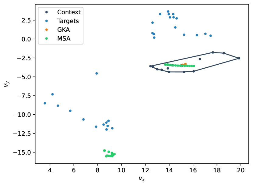
(a) Context, targets, and forecast in wind speed space.

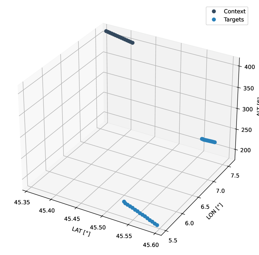
(b) Context and targets in the 3D space.

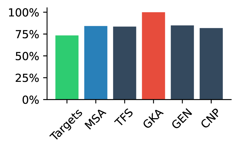
(c) Percentage of the prediction values that are contained in the convex hull of the measurement in the context in percent.

Figure 9: Context and targets represented in wind speed and 3D space. Both the context and targets correspond to 1-minute slices of data. The targets capture wind measurements recorded 30 minutes following the context data. Additionally, the forecasts generated by the MSA and GKA models are depicted. Notably, the GKA model is confined to predicting within the convex hull of the context values, which is visually highlighted in grey. Conversely, the MSA model is unrestricted by this limitation and can make predictions beyond the convex hull of the context values.

10.1 Decoder and conditioning function

In the main paper, we presented a comparison of the key distinctions between our attention-based architectures. However, it could be that the performance differences observed could be attributed to minor variations in the architecture design. For the sake of completeness, in this section, we provide experimental results to address this aspect by comparing the remaining differences between GEN and TFS. Specifically, we focus on analyzing the impact of the number of decoder layers and the conditioning function. It is important to note that this analysis does not apply to MSA, as it does not possess an encoder-decoder structure.

GEN and TFS differ not only in their latent representation but also on two other points: (1) the way that they access the encoded information in the decoder and (2) how much computing power is used in the decoder stack.

In all three models, we tried using either a distance-based function or cross-attention to combine the target position with the encoded latents. CNP concatenate the same context vector to all target queries, which we model as equivalent to averaging the latents based on the distance in the case that there is only one latent.

Specifically, each latent is associated with a position $\mathbf{l}_{x}$ in the underlying space with corresponding value $\mathbf{l}_{y}$. Conditioning is made by averaging the latent features based on their distance with the query $\mathbf{t}_{x}$. Its formula is given by:

$$z=\sum_{\mathbf{l}\in\text{latents}}r(\text{dist}(\mathbf{l}_{x},\mathbf{t}_{x}))\mathbf{l}_{y}$$ (5)

Where $r:\mathbb{R}\rightarrow[0,1]$ is a function that maps distances to weights, and $\mathbf{l}_{x}$ represents the position associated with the latent nodes with value $\mathbf{l}_{y}$. This vector $z$ is then concatenated to the target position $\mathbf{t}_{x}$ and fed to the decoder which is a MLP in this case.

GEN use this distance-based aggregation function by default whereas TFS uses cross-attention. We tried using cross-attention for CNP and GEN and using the same distance-based aggregating function for TFS using the distance between context position and target position as a reference for this scheme. For GEN and CNP using cross-attention give approximately the same results, but using distance-based conditioning for TFS hurts the performance significantly.

Table 4: Results of the ablation of the conditioning function used to combine the latents with the target position. We adapted the architecture so that they used both a distance-based conditioning function, which combines the query position with a weighted average of the nearest latents and standard cross-attention. We show in italics hybrid architecture where we had to switch the default conditioning method. For GEN and CNP replacing the conditioning method does not impact the performance, but for TFS switching to a distance-based conditioning function impacts the performance drastically.

Model	Distance- based	Cross- attention
CNP	.115 $\pm$ .015	.119 $\pm$ .014
GEN	.024 $\pm$ .004	.022 $\pm$ .006
TFS	.042 $\pm$ .023	.020 $\pm$ .011

We also ran ablations that created hybrid cases for both transformers and GEN and concluded that adding decoding layers helped TFS to reach better performance. Adding layers to the GEN decoder drastically reduces model performance, which seems to be coherent with the fact that GEN were shown to be more prone to overfitting in the results section.

Finally, we want to highlight that MSA outperforms all the models presented in this section by a large margin section 7.

Table 5: Results of the decoder-layer ablation. One difference between TFS and GEN is that by default TFS use multiple layers in its decoder whereas GEN uses one, and delegates all processing to the encoder. We see that having multiple decoder layers helps the transformer whereas it impacts the performance of the GEN.

	# Decoder layers
Model	1	2	4
GEN	.021 $\pm$ .002	.040 $\pm$ .012	.106 $\pm$ .004
TFS	.020 $\pm$ .011	.019 $\pm$ .005	.013 $\pm$ .001

11 Wind nowcasting metrics

This section defines the metrics used for wind nowcasting.

Root Mean Square Error (RMSE)

It takes the square root of the square distance between the prediction and the output. It has the advantage of having the same units as the forecasted values.

$$\text{RMSE}(\hat{t},t)=\sqrt{\frac{\sum_{k}^{N}(\hat{t}_{k}-t_{k})^{2}}{N}}$$ (6)

Mean Absolute Error for angle (angle MAE)

It is interesting and sometimes more insightful to decompose the error made by the models in their angular and norm components. This is the role of this metric and the following.

$$\text{angle MAE}(\hat{t},t)=||(\alpha(\hat{t})-\alpha(t))||_{L_{1}}$$ (7)

where $\alpha\left(\vec{x}=\begin{pmatrix}x\\ y\end{pmatrix}\right)=\arctan(y,x)*\frac{360}{2\pi}$

Mean Absolute Error for norm (norm MAE)

Following the explanation of the last paragraph:

$$\text{norm MAE}(\hat{t},t)=\sum_{k}\,|\mid\mid\hat{t}_{k}\mid\mid_{2}-\mid\mid t_{k}\mid\mid_{2}|$$ (8)

Relative Bias (rel BIAS) x,y

Additionally, we used weather metrics as in [9]. The relative bias measure if the considered model under or overestimate one quantity. It is defined as:

$$\text{rel BIAS}(\hat{t},t)=\frac{\text{mean}(\hat{t}_{k}-t_{k})}{\text{mean}(\hat{t}_{k})}$$ (9)

Ratio of standard deviation (rSTD)

The ratios of standard deviation indicate whether the dispersion of the output of the model matches the target distribution. It has an optimal value of $1$.

$$\text{rSTD}(\hat{t},t)=\frac{\text{std}(\hat{t})}{\text{std}(t)}$$ (10)

NSE

The last domain metric used is the Nash-Sutcliffe efficiency (NSE), which compares the error of the model with the average of the target data. A score of 1 is ideal and a negative score indicates that the model was worse than the average prediction on average.

$$\text{NSE}(\hat{t},t)=1-\frac{\text{MSE}(\hat{t},t)}{\text{MSE}(t,\text{mean(t)})}$$ (11)

12 Influence of the tightness of the measurements on the performances

To evaluate the influence of the tightness of the measurements on the results we designed the following experiment: We start with a pair of context $(c_{x},c_{y})$ and target points $(t_{x},t_{y})$. We pick one point from the context and restrict the context to a small number of measurements close to this point. Then, we calculate the error made by the model when it is given only this restricted context and rank them by their distance to the context’s center. As the dimensions (longitude, latitude, altitude) differ, we first normalized the data along each axis. We repeat this process and average the results.

Table 6: Influence of the tightness of the measurements on the performance. We restrict the context to measurements that are close to the query point and then measure the error as a function of the distance from this query point averaged over the whole dataset. We estimate the standard deviation using three random seeds.

Normalized Dist	MSA	TFS
0.5–1.0	5.56 $\pm$ 0.49	7.73 $\pm$ 0.37
1.0–1.5	6.62 $\pm$ 0.35	7.35 $\pm$ 0.53
1.5–2.0	7.57 $\pm$ 0.43	7.87 $\pm$ 0.36
2.0–2.5	9.52 $\pm$ 0.47	9.48 $\pm$ 0.66
2.5–end	10.35 $\pm$ 0.49	10.53 $\pm$ 0.61

We see that the error increases with the distance to the context. Now in practice, the context is not restricted and contains points all over the space (so the mean minimum normalized distance to the target points is usually often below 1.0)

We assessed general uncertainty by training the model using various random seeds, resulting in an ensemble of models from which we can determine the standard deviation and added it to the results table of the previous experiment.

13 Influence of the target positions

In this section, we assess the impact of the target position on the training of the MSA model.

The context data for the Poisson equation is heavily prescribed (where context points belonged to the source or sink or boundary conditions), while for the Darcy Flow equation, we constructed a similarly-shaped data set by subsampling the data set from [1] to create the context and targets. Thus, the Darcy flow test problem gives an ideal testbed for examining the influence of target positions on the training. To examine the impact of the context position, we designed an additional experiment where we sampled the context from the bottom left quadrant of the unit cube and the targets from the upper right quadrants of the unit cube. We conduct our analysis for small (5k parameters) and large (100k parameters) models. We report the test loss as a function of the percentage of the context from the upper-right quadrants (where all targets are located, the remaining from the bottom-left quadrant).

Table 7: Influence of the target position on the training. We report the test error for the MSA model at two different sizes. We devised an experiment in which we extracted the context from the bottom left quadrant of the unit cube, while the targets were sampled from the upper right quadrants of the same unit cube.

	0%	2%	25%	50%	100%
MSA 5k	0.14	0.15	0.14	0.09	0.03
MSA 100k	0.14	0.14	0.13	0.09	0.03

In the first column (0% of the data from the first quadrant), we see that the MSA model struggled to learn when the context and targets are disjoint. The error improves with greater overlaps between context and target, with p = 100% corresponding to the case in the paper (albeit on one-quarter of the data). Similar dynamics hold for both model sizes. We believe that this is due to the Darcy Flow simulation being highly location-dependent, as can be seen in some examples from the dataset fig. 7(a).

Regarding the training performance, we noticed no substantial difference in the total time to a solution, they all took approximately 1000 epochs in all cases. Larger models were always able to overfit the data.

Table 8: Influence of the target position on the training. We report the train error for the MSA model at two different sizes. Both models were able to overfit the data.

	0%	2%	25%	50%	100%
MSA 5k	0.07	0.07	0.07	0.05	0.02
MSA 100k	0.00	0.00	0.00	0.00	0.00

14 Difference between MSA and TFS

Initially, we explored an encoder-decoder architecture adapted from Vaswani et al. [26]. Following the similar logic that led to the development of encoder-only models, we then tried our multilayer self-attention model (MSA), which uses a transformer encoder stack adapted from Devlin et al. [4].

We believe this design is superior for two main reasons: Firstly, the model maintains only one path, which contains residual connections all the way from the encoded input to the target, unlike the encoder-decoder architecture. In the encoder-decoder architecture, cross-attention has two main residual paths: one from the encoder and one from the decoder. However, the residual connection of the encoder path ends at the cross-attention layer.

Secondly, MSA’s architecture is considerably simpler as it only requires two components: self-attention and MLPs (Multi-Layer Perceptrons).

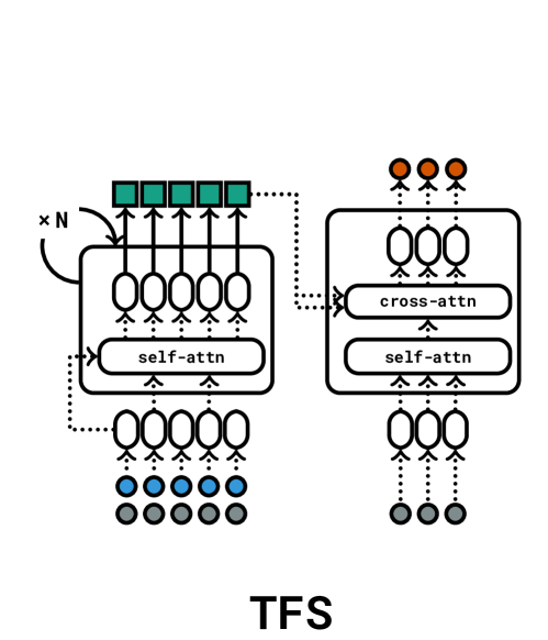
(a) Transformer, Ours based on [26]

(b) Multilayer Self-Attention (Ours)

Figure 10: Comparison between TFS and MSA architecture.

15 Different Message Passing Scheme

We try here different message-passing schemes even one using attention, to help us demonstrate the fact that the whole family of models that encodes the space as a single graph suffers from the same bottlenecking effect. Here are the results of the wind nowcasting task:

Table 9: Performance of GEN with different message passing schemes for the wind nowcasting task. Various message-passing schemes, including those with attention, were explored using PyTorch Geometric [6]. The best-performing GEN model with the default message-passing scheme is indicated with a reference line. While certain schemes showed improvements over GEN’s performance, the overall performance remained relatively consistent and was still outperformed by MSA. For additional information on the different message-passing schemes and related references, please refer to the PyTorch Geometric documentation.

Model	Score
TransformerConv	9.2830
GATv2Conv	9.3353
GeneralConv	9.3699
GATConv	9.7744
SAGEConv	9.7837
ARMAConv	9.8391
TAGConv	9.8653
SGConv	9.9465
SuperGATConv	10.0961
GCNConv	10.1344
LEConv	10.6062
GENConv	23.9847

Although certain message-passing schemes enhance the performance of the GEN model, it still falls short of the performance achieved by MSA. We attribute this difference to the bottlenecking effect caused by the latent graph. For additional information on the various message-passing schemes and relevant references, please consult the PyTorch Geometric documentation available at https://pytorch-geometric.readthedocs.io/en/latest/modules/nn.html#convolutional-layers.

16 Broader Impacts

We do not anticipate any significant adverse effects on society due to this work. Generally, having an additional method for weather nowcasting may lead to an increase in computational resources required, but this is a common consequence of many deep learning systems.

We believe that enhancing the reliability of weather forecasts and dynamical systems has a more positive impact on society. By improving the accuracy and precision of these predictions, we can provide valuable information for various sectors, such as agriculture, transportation, disaster management, and overall planning and decision-making processes.

17 Limitations

Our method, like other attention-based models, suffers from quadratic scaling. In the case of MSA, it is slightly more computationally intensive compared to TFS due to the combination of target and context in the same sequence. This results in an attention mechanism that scales with $\mathcal{O}((N_{c}+N_{t})^{2})$, which is asymptotically equivalent to the scaling of transformers, which is $\mathcal{O}(N_{c}^{2}+N_{t}^{2}+N_{c}N_{t})$, but in practice introduces an additional $N_{c}N_{t}$ term. However, in all our experiments, this computational overhead did not pose a problem. We acknowledge the issue in the scaling of the model and refer to possible solutions outlined in the related work to address this challenge.

Another drawback of this study is the absence of a comparison between the models and other established models used for modeling dynamical systems on a grid, as discussed in the work by Li et al. [18]. We anticipate that our approach may not perform as effectively as competing models on grids due to two reasons. Firstly, the previously mentioned scaling issue becomes significant when dealing with larger grid sizes, such as $1024\times 1024$ grids. Additionally, our approach lacks certain inductive biases that aid in grid-based modeling. Nonetheless, we believe that attention-based models still hold promise for grid-based systems, as demonstrated by the success of Vision Transformers (ViT) in other domains[5]. However, tokenization may be necessary for their effective implementation.

18 Experiment and training details

In this supplementary material, we provide the code required to process the dataset and reproduce the experiments. We utilized Hydra as a configuration manager [27] and include the precise configuration for each case. The experiments were executed multiple times on a GPU cluster, but each experiment can be conducted on a single GPU in a relatively short timeframe, ranging from a few hours to a maximum of a few days.

19 Error Bars

We ran multiple runs of our experiments and report the standard deviation in all concerned tables.

20 Amount of Compute needed to replicate the experiments

Training smaller models (5k, 20k) usually takes a few hours. Training larger models (except for CNP which is considerably faster) runs in at most two GPU days. We estimate the number of GPU days to replicate all experiments for all models to be on the order of 100 GPU days.

21 Reproductibility

We provide the link to the dataset and the whole code base for processing it and running the experiments.

22 Licenses

All concerned databases are openly accessible on the web and have permissive licenses, we give a link to each dataset in table 3

References

- Alet et al. [2019] Ferran Alet, Adarsh Keshav Jeewajee, Maria Bauza Villalonga, Alberto Rodriguez, Tomas Lozano-Perez, and Leslie Kaelbling. Graph element networks: adaptive, structured computation and memory. In International Conference on Machine Learning, pages 212–222. PMLR, 2019.
- Dao et al. [2022] Tri Dao, Daniel Y Fu, Stefano Ermon, Atri Rudra, and Christopher Re. Flashattention: Fast and memory-efficient exact attention with IO-awareness. In Alice H. Oh, Alekh Agarwal, Danielle Belgrave, and Kyunghyun Cho, editors, Advances in Neural Information Processing Systems, 2022. URL https://openreview.net/forum?id=H4DqfPSibmx.
- Dettmers et al. [2022] Tim Dettmers, Mike Lewis, Younes Belkada, and Luke Zettlemoyer. GPT3.int8(): 8-bit matrix multiplication for transformers at scale. In Alice H. Oh, Alekh Agarwal, Danielle Belgrave, and Kyunghyun Cho, editors, Advances in Neural Information Processing Systems, 2022. URL https://openreview.net/forum?id=dXiGWqBoxaD.
- Devlin et al. [2019] Jacob Devlin, Ming-Wei Chang, Kenton Lee, and Kristina Toutanova. BERT: pre-training of deep bidirectional transformers for language understanding. In Jill Burstein, Christy Doran, and Thamar Solorio, editors, Proceedings of the 2019 Conference of the North American Chapter of the Association for Computational Linguistics: Human Language Technologies, NAACL-HLT 2019, Minneapolis, MN, USA, June 2-7, 2019, Volume 1 (Long and Short Papers), pages 4171–4186. Association for Computational Linguistics, 2019. doi: 10.18653/v1/n19-1423. URL https://doi.org/10.18653/v1/n19-1423.
- Dosovitskiy et al. [2020] Alexey Dosovitskiy, Lucas Beyer, Alexander Kolesnikov, Dirk Weissenborn, Xiaohua Zhai, Thomas Unterthiner, Mostafa Dehghani, Matthias Minderer, Georg Heigold, Sylvain Gelly, et al. An image is worth 16x16 words: Transformers for image recognition at scale. arXiv preprint arXiv:2010.11929, 2020.
- Fey and Lenssen [2019] Matthias Fey and Jan E. Lenssen. Fast graph representation learning with PyTorch Geometric. In ICLR Workshop on Representation Learning on Graphs and Manifolds, 2019.
- Garnelo et al. [2018] Marta Garnelo, Dan Rosenbaum, Christopher Maddison, Tiago Ramalho, David Saxton, Murray Shanahan, Yee Whye Teh, Danilo Rezende, and S. M. Ali Eslami. Conditional neural processes. In Jennifer Dy and Andreas Krause, editors, Proceedings of the 35th International Conference on Machine Learning, volume 80 of Proceedings of Machine Learning Research, pages 1704–1713. PMLR, 10–15 Jul 2018. URL https://proceedings.mlr.press/v80/garnelo18a.html.
- Geneva and Zabaras [2022] Nicholas Geneva and Nicholas Zabaras. Transformers for modeling physical systems. Neural Networks, 146:272–289, 2022.
- Ghiggi et al. [2019] G. Ghiggi, V. Humphrey, S. I. Seneviratne, and L. Gudmundsson. Grun: an observation-based global gridded runoff dataset from 1902 to 2014. Earth System Science Data, 11(4):1655–1674, 2019. doi: 10.5194/essd-11-1655-2019. URL https://essd.copernicus.org/articles/11/1655/2019/.
- Gupta and Brandstetter [2022] Jayesh K. Gupta and Johannes Brandstetter. Towards multi-spatiotemporal-scale generalized pde modeling, 2022. URL https://arxiv.org/abs/2209.15616.
- Hersbach et al. [2023] Hans Hersbach, Barbara Bell, Paul Berrisford, Giovanni Biavati, András Horányi, Joaquín Muñoz Sabater, Julien Nicolas, Carole Peubey, Razvan Radu, Ivan Rozum, Dries Schepers, Adrian Simmons, Cornel Soci, Dick Dee, and Jean-Noël Thépaut. ERA5 hourly data on single levels from 1940 to present. Copernicus Climate Change Service (C3S) Climate Data Store (CDS), 2023. Accessed on 17-05-2023.
- Jaegle et al. [2021] Andrew Jaegle, Sebastian Borgeaud, Jean-Baptiste Alayrac, Carl Doersch, Catalin Ionescu, David Ding, Skanda Koppula, Daniel Zoran, Andrew Brock, Evan Shelhamer, et al. Perceiver io: A general architecture for structured inputs & outputs. arXiv preprint arXiv:2107.14795, 2021.
- Katharopoulos et al. [2020] Angelos Katharopoulos, Apoorv Vyas, Nikolaos Pappas, and François Fleuret. Transformers are RNNs: Fast autoregressive transformers with linear attention. In Hal Daumé III and Aarti Singh, editors, Proceedings of the 37th International Conference on Machine Learning, volume 119 of Proceedings of Machine Learning Research, pages 5156–5165. PMLR, 13–18 Jul 2020. URL https://proceedings.mlr.press/v119/katharopoulos20a.html.
- Kim et al. [2019] Hyunjik Kim, Andriy Mnih, Jonathan Schwarz, Marta Garnelo, Ali Eslami, Dan Rosenbaum, Oriol Vinyals, and Yee Whye Teh. Attentive neural processes. In International Conference on Learning Representations, 2019. URL https://openreview.net/forum?id=SkE6PjC9KX.
- Lam et al. [2022] Remi Lam, Alvaro Sanchez-Gonzalez, Matthew Willson, Peter Wirnsberger, Meire Fortunato, Alexander Pritzel, Suman Ravuri, Timo Ewalds, Ferran Alet, Zach Eaton-Rosen, Weihua Hu, Alexander Merose, Stephan Hoyer, George Holland, Jacklynn Stott, Oriol Vinyals, Shakir Mohamed, and Peter Battaglia. Graphcast: Learning skillful medium-range global weather forecasting, 2022. URL https://arxiv.org/abs/2212.12794.
- Lee et al. [2019] Juho Lee, Yoonho Lee, Jungtaek Kim, Adam R Kosiorek, Seungjin Choi, and Yee Whye Teh. Set transformer. In International Conference on Machine Learning, 2019.
- Li et al. [2019] Shiyang Li, Xiaoyong Jin, Yao Xuan, Xiyou Zhou, Wenhu Chen, Yu-Xiang Wang, and Xifeng Yan. Enhancing the locality and breaking the memory bottleneck of transformer on time series forecasting. Advances in neural information processing systems, 32, 2019.
- Li et al. [2021] Zongyi Li, Nikola Borislavov Kovachki, Kamyar Azizzadenesheli, Burigede Liu, Kaushik Bhattacharya, Andrew Stuart, and Anima Anandkumar. Fourier neural operator for parametric partial differential equations. In International Conference on Learning Representations, 2021. URL https://openreview.net/forum?id=c8P9NQVtmnO.
- Narang et al. [2021] Sharan Narang, Hyung Won Chung, Yi Tay, Liam Fedus, Thibault Févry, Michael Matena, Karishma Malkan, Noah Fiedel, Noam Shazeer, Zhenzhong Lan, Yanqi Zhou, Wei Li, Nan Ding, Jake Marcus, Adam Roberts, and Colin Raffel. Do transformer modifications transfer across implementations and applications? In EMNLP (1), pages 5758–5773. Association for Computational Linguistics, 2021.
- Pannatier et al. [2021] Arnaud Pannatier, Ricardo Picatoste, and François Fleuret. Efficient wind speed nowcasting with gpu-accelerated nearest neighbors algorithm, 2021. URL https://arxiv.org/abs/2112.10408.
- Pfaff et al. [2020] Tobias Pfaff, Meire Fortunato, Alvaro Sanchez-Gonzalez, and Peter Battaglia. Learning mesh-based simulation with graph networks. In International Conference on Learning Representations, 2020.
- Radford et al. [2018] Alec Radford, Karthik Narasimhan, Tim Salimans, Ilya Sutskever, et al. Improving language understanding by generative pre-training. 2018.
- Radford et al. [2022] Alec Radford, Jong Wook Kim, Tao Xu, Greg Brockman, Christine McLeavey, and Ilya Sutskever. Robust speech recognition via large-scale weak supervision. arXiv preprint arXiv:2212.04356, 2022.
- Shi et al. [2017] Xingjian Shi, Zhihan Gao, Leonard Lausen, Hao Wang, Dit-Yan Yeung, Wai-kin Wong, and Wang-chun Woo. Deep Learning for Precipitation Nowcasting: A Benchmark and A New Model. Advances in Neural Information Processing Systems, 2017.
- Suman et al. [2021] R. Suman, L. Karel, W. Matthew, K. Dmitry, L. Remi, M. Piotr, F. Megan, A. Maria, K Sheleem, M. Sam, P. Rachel, M. Amol, C. Aidan, B. Andrew, S. Karen, H. Raia, R. Niall, C. Ellen, A. Alberto, and M. Shakir. Skilful precipitation nowcasting using deep generative models of radar. Nature, 597(7878):672–677, 09 2021. ISSN 1476-4687. doi: 10.1038/s41586-021-03854-z. URL https://doi.org/10.1038/s41586-021-03854-z.
- Vaswani et al. [2017] Ashish Vaswani, Noam Shazeer, Niki Parmar, Jakob Uszkoreit, Llion Jones, Aidan N Gomez, Łukasz Kaiser, and Illia Polosukhin. Attention is all you need. Advances in neural information processing systems, 30, 2017.
- Yadan [2019] Omry Yadan. Hydra - a framework for elegantly configuring complex applications. Github, 2019. URL https://github.com/facebookresearch/hydra.
- Zaheer et al. [2017] Manzil Zaheer, Satwik Kottur, Siamak Ravanbakhsh, Barnabás Póczos, Ruslan Salakhutdinov, and Alexander J. Smola. Deep sets. CoRR, abs/1703.06114, 2017. URL http://arxiv.org/abs/1703.06114.