Cutting-plane algorithms for preemptive uniprocessor real-time scheduling problems

Abstract.

Fixed-point iteration algorithms like RTA (response time analysis) and QPA (quick processor-demand analysis) are arguably the most popular ways of solving schedulability problems for preemptive uniprocessor FP (fixed-priority) and EDF (earliest-deadline-first) systems. Several IP (integer program) formulations have also been proposed for these problems, but it is unclear whether the algorithms for solving these formulations are related to RTA and QPA. By discovering connections between the problems and the algorithms, we show that RTA and QPA are, in fact, suboptimal cutting-plane algorithms for specific IP formulations of FP and EDF schedulability, where optimality is defined with respect to convergence rate. We propose optimal cutting-plane algorithms for these IP formulations. We compare the new algorithms with RTA and QPA on large collections of synthetic systems to gauge the improvement in convergence rates and running times.

Key words and phrases: hard real-time scheduling, fixed priority, earliest deadline first, cutting planes, linear programming duality, fixed-point iteration

1. Introduction

FP (fixed-priority) and EDF (earliest-deadline-first) are two popular methods of assigning priorities to preemptible hard real-time tasks in a uniprocessor priority-driven system. In FP systems, each task is assigned a priority that remains constant during execution; in contrast, priorities of tasks in EDF systems are variable during execution, and at any instant a task with the earliest deadline has the highest priority. From the early work of Liu and Layland (1973), it has been known that the two systems are quite different: for instance, an implicit-deadline FP system can violate its timing requirements even when processor utilization is as low as 70%, while a comparable EDF system is safe for all processor utilizations up to 100%. Preemptive uniprocessor systems with FP and EDF priority assignments are some of the most well-studied systems in hard real-time scheduling theory: historical perspectives on these systems and other supporting literature may be found in surveys, handbooks, and textbooks (Audsley et al., 1995; Liu, 2000; Sha et al., 2004; Buttazzo, 2011; Levy and Tian, 2020); works that study the differences between FP and EDF systems are also available (Buttazzo, 2005; Rivas et al., 2011; Perale and Vardanega, 2021).

Systems that do not violate their timing requirements are called safe or schedulable; other systems are said to be unschedulable. A schedulable system is often characterized by a schedulability condition: for instance, a schedulable constrained-deadline preemptive uniprocessor FP system with $n$ tasks listed in nonincreasing order of priority is characterized by the existence of a $t\in\linterval{0}{D_{i}}$ such that $\operatorname{rbf}_{i}(t)\leq t$ for all $i\in[n]$, where $D_{i}$ is the relative deadline of the task $i$ and $\operatorname{rbf}_{i}$ maps any $t$ to the maximum amount of work generated by the subsystem $[i]$ in any interval of length $t$ (Joseph and Pandya, 1986; Lehoczky et al., 1989). An unschedulable arbitrary-deadline preemptive uniprocessor EDF system with $n$ tasks can also be characterized by the existence of a $t\in\linterval{0}{\operatorname{lcm}_{j\in[n]}T_{j}}$ such that $\operatorname{dbf}(t)>t$ where $T_{j}$ is the period of task $j$ and $\operatorname{dbf}$ maps any $t$ to the amount of work generated by the system in the interval that must be completed in the interval (Baruah et al., 1990b; Ripoll et al., 1996). We will discuss schedulability conditions, relative deadlines, constrained deadlines, arbitrary deadlines, $\operatorname{rbf}$, periods and $\operatorname{dbf}$ in more detail in a later section. For now, it suffices to know that the schedulability conditions for both FP and EDF systems are about the existence of a $t$ in a bounded interval where some function of $t$ is nonnegative; for FP (resp., EDF) systems, the function is $t\mapsto t-\operatorname{rbf}_{i}(t)$ (resp., $t\mapsto\operatorname{dbf}(t)-t-1$).

Given a description of a hard real-time system, the problem of deciding whether the given system satisfies its timing requirements is called a schedulability problem. An algorithm that solves a schedulability problem is called a schedulability test. Given a system, a schedulability test checks whether the appropriate schedulability condition holds for the system.

An FP schedulability test attempts to find a $t\in\linterval{0}{D_{i}}$ where $\operatorname{rbf}_{i}(t)\leq t$. There are many algorithmic techniques that can be used to achieve this goal: for example, we can use fixed-point iteration (Joseph and Pandya, 1986; Audsley et al., 1993), depth-bounded search trees (Manabe and Aoyagi, 1998; Bini and Buttazzo, 2004), and continued fractions (Park and Baek, 2023). The fixed-point iteration test is called RTA (response time analysis), and the depth-bounded search tree test is called HET (hyperplanes exact test). The running times of these tests are, in general, incomparable: the most significant factor in the worst-case running time of RTA is $D_{\max}/T_{\min}$ where $D_{\max}$ (resp., $T_{\min}$) is the largest deadline (resp., the smallest period) in the system; the most significant factor in the worst-case running time of HET is $2^{\text{\#periods}}$. Thus, for hard problem instances where the number of periods is small but $D_{\max}/T_{\min}$ is large, HET will likely outperform RTA; on the other hand, for hard problem instances where the number of periods is large and $D_{\max}/T_{\min}$ is small, RTA will likely outperform HET.

Similarly, given a system that is not trivially unschedulable an EDF schedulability test attempts to find a $t\in\ointerval{0}{\operatorname{lcm}_{j\in[n]}T_{j}}$ such that $\operatorname{dbf}(t)>t$. Many algorithmic approaches can be used to search for $t$ including fixed-point iteration (Zhang and Burns, 2009b), integer programming in fixed dimension (Baruah et al., 1990a) (utilizing Lenstra’s algorithm (Lenstra, 1983)), and convex-hull computation (Bini, 2019). The fixed-point iteration algorithm is called QPA (quick processor-demand analysis). As was the case with FP schedulability tests, the running times of EDF schedulability tests are not comparable, in general: the most significant factor in the worst-case running time of QPA is $\operatorname{lcm}_{j\in[n]}T_{j}/T_{\min}$; the most significant factor in the worst-case running time of Lenstra’s algorithm is $p^{\mathcal{O}(p)}$ where $p$ is the variety of the system. Thus, for hard problem instances where the variety is very small and $\operatorname{lcm}_{j\in[n]}T_{j}/T_{\min}$ is large, Lenstra’s algorithm will likely outperform QPA; in contrast, for hard problem instances where the ratio is small and the variety is large, QPA will likely outperform Lenstra’s algorithm. Differences in worst-case running times for various algorithmic approaches for FP and EDF schedulability tests with respect to the sizes of different problem parameters such as the number of periods in the system, the variety of the system, $D_{\max}/T_{\min}$, and $\operatorname{lcm}_{j\in[n]}T_{j}/T_{\min}$ have been studied recently using the framework of parameterized algorithms by Baruah et al. (2022).

Although applying new algorithmic techniques to create new schedulability tests with better properties is very important, it is equally important to attempt to understand the relationships between the schedulability problems and between the algorithms for the problems. Efforts in the latter direction often yield new structural and algorithmic insights and result in a coherent unified theory. We are interested in studying the connections between the FP schedulability problem and the EDF schedulability problem in the context of four algorithmic approaches:

RTA:

the fixed-point iteration algorithm for FP schedulability (see Section 2.1).

IP-FP:

the IP (integer programming) formulation for FP schedulability where the variables correspond to the integral quantities in $\operatorname{rbf}_{i}$ (see Section 4.1).

QPA:

the fixed-point iteration algorithm for EDF schedulability (see Section 2.2).

IP-EDF:

the IP formulation for EDF schedulability where the variables correspond to the integral quantities in $\operatorname{dbf}$ (see Section 4.2).

While RTA and QPA are well-known, IP-FP and IP-EDF are nonstandard names that we are using to refer to specific IP formulations of the schedulability problems described later in the document; moreover, IP-FP and IP-EDF qualify only vaguely as algorithmic approaches because we have not specified an algorithm for solving the IP formulations yet (we will design a new cutting-plane algorithm to solve the IPs in a unified manner).

It is natural to try to understand the relationships within the pairs (RTA, IP-FP) and (QPA, IP-EDF) because they solve the FP schedulability problem and the EDF schedulability problem respectively. However, we found that studying the problems separately is a little inefficient because both problems can be reduced in polynomial time to a common problem called the kernel (see Section 5):

If the kernel can be solved efficiently by some algorithm, then both FP schedulability and EDF schedulability can be solved efficiently; thus, the kernel captures the essence of the hardness of the two problems. We prove the following facts about the kernel:

• The kernel can be solved by a fixed-point iteration algorithm called FP-KERN (see Section 5.1). RTA and QPA can be recovered from FP-KERN by composing it with the above reductions.

• The kernel has an IP formulation called IP-KERN (see Section 5.2). IP-FP and IP-EDF can be recovered from IP-KERN by composing it with the above reductions.

Since any relationship between FP-KERN and IP-KERN must also exist for RTA (resp., QPA) and IP-FP (resp., IP-EDF), we can focus our attention on FP-KERN and IP-KERN.

Our main result is that IP-KERN can be solved by a family of cutting-plane algorithms; FP-KERN is a member of the family but it is not the optimal algorithm in this family with respect to convergence rate, which is defined as the inverse of the number of iterations required for convergence; and the optimal algorithm in the family, called CP-KERN, has a better convergence rate than FP-KERN. Viewed from the FP (resp., EDF) perspective, RTA (resp., QPA) is a suboptimal cutting-plane algorithm and CP-KERN converges to the solution in fewer iterations. In our empirical evaluation, we compare the number of iterations required by the fixed-point iteration algorithms (RTA and QPA) and CP-KERN on synthetic systems; the results confirm that CP-KERN has a better convergence rate than RTA and QPA.

1.1. Practical concerns: computational complexity

Faster schedulability algorithms are needed in many applications. In holistic analyses of distributed real-time systems, schedulability tests are called a great many times till the values for all parameters in the system stabilize or an unschedulable subsystem is discovered (Tindell and Clark, 1994; Spuri, 1996b). In partitioned approaches to multiprocessor scheduling, uniprocessor schedulability tests are used to determine the feasibility of (usually numerous) partitions. In automatic or interactive design space explorations to optimize objectives such as energy consumption, schedulability tests are used to determine the feasibility of numerous configurations. The speed of a schedulability test is also crucial when it is used as an online test in a dynamic embedded system.

While the convergence rate of CP-KERN is better than FP-KERN (think, RTA and QPA), this does not imply that CP-KERN is faster than FP-KERN. Consider, for instance, the center of gravity method for convex programs (see, for instance, Bubeck, 2015, Sec. 2.1). The center of gravity method has a good convergence rate, but it requires the center of gravity of a convex body to be computed in each iteration for which no efficient procedures are known. CP-KERN, unlike the center of gravity method, is not purely theoretical. In each iteration of CP-KERN we must solve a linear relaxation of IP-KERN. Since linear programs can be solved in polynomial time by the ellipsoid method (Khachiyan, 1980) and interior point methods (Karmarkar, 1984), each iteration of CP-KERN has polynomial running time.

To solve linear relaxations of IP-KERN in each iteration of CP-KERN even more efficiently, we propose a specialized method that runs in strongly polynomial time. Since no strongly polynomial-time algorithms are known for linear programming, our specialized method is an improvement over using a general algorithm for solving linear programs. Moreover, we show that if CP-KERN uses this specialized method then it has the same worst-case running time as FP-KERN. This result, combined with the optimality with respect to convergence rate, establishes CP-KERN as a better algorithm than FP-KERN in theory. In practice, FP-KERN may be faster than CP-KERN for instances where the difference in convergence rates of CP-KERN and FP-KERN is negligible because FP-KERN does less work in each iteration than CP-KERN when we do not ignore constant factors. We compare the running times on synthetic systems in our empirical evaluation.

1.2. Practical concerns: implementation complexity

Since FP-KERN proceeds by fixed-point iteration, it is quite easy to implement without depending on external libraries; thus, it is well-suited to serve as an online schedulability test in a dynamic embedded system where task and resource constraints are subject to change over time. Since a cutting-plane algorithm for an IP solves a linear program in each iteration, an implementation of a cutting-plane algorithm for solving general IPs usually depends on linear programming libraries, commercial or otherwise, making it harder to deploy on dynamic embedded systems. When CP-KERN utilizes our specialized algorithm to solve relaxations of IP-KERN, it is about 50 lines in pseudocode, it uses elementary arithmetic operations, and does not depend on mathematical programming or algebra libraries in function calls. Therefore, CP-KERN has a small footprint and is well-suited for deployment on dynamic embedded systems. For software developers writing a schedulability library, our structured approach promotes code reuse and reduces development effort. Moreover, the smaller codebase inspires more trust in stakeholders.

2. System Models

In a hard real-time system, a task receives an infinite stream of requests and it must respond to each request within a fixed amount of time. We consider a system comprising $n$ independent preemptible sporadic tasks, labeled $1,2,\dotsc,n$. We refer to the system simply as $[n]$; given a system $[n]$, $i\in[n]$ is the $i$-th task, and $[i]\subseteq[n]$ is a subsystem of $[n]$ that contains tasks $\{1,2,\ldots,i\}$. Each sporadic task $i\in[n]$ has the following (integral) characteristics:

Symbol	Task Characteristic
$C_{i}$	worst-case execution time (wcet)
$T_{i}$	minimum duration between successive request arrivals (period)
$D_{i}$	maximum duration between request arrival and response (relative deadline)
$J_{i}$	maximum duration between request arrival and the task becoming eligible for execution (release jitter)

If the $k$-request for task $i$ arrives at time $t$, then the following statements must be true:

• The request must be completed by time $t+D_{i}$ in a feasible schedule; $t+D_{i}$ is the absolute deadline for the completion of the response to the request.

• The $(k+1)$-th request for task $i$ cannot arrive before $t+T_{i}$.

Sometimes a request may arrive at time $t$ and the task may not become eligible for execution until time $t+\delta$ where $\delta>0$; $\delta$ is the release jitter experienced by task $i$ at time $t$, and $J_{i}$ is the maximum release jitter that can be experienced by task $i$.

If $D_{i}=T_{i}$, then the deadline $D_{i}$ is said to be implicit; if $D_{i}\leq T_{i}$, then the deadline $D_{i}$ is said to be constrained. If all tasks in a system have implicit deadlines, then the system is an implicit-deadline system. If all tasks in a system have constrained deadlines, then the system is a constrained-deadline system; otherwise, it is an arbitrary-deadline system.

We refer to the largest (resp., smallest) period in the system by $T_{\max}$ (resp., $T_{\min}$); similar symbols are used for other task parameters as well. We refer to the harmonic mean of the periods by $T_{\mathrm{hm}}$.

As mentioned in Section 1, we assume that the tasks are preemptible, run on a single processor, and are scheduled by an FP or EDF scheduler.

2.1. FP schedulability and RTA

We restrict our attention to synchronous constrained-deadline preemptive uniprocessor FP systems, and we simply call them FP systems. We assume that tasks are listed in decreasing order of priority in FP systems.

An FP system $[n]$ is schedulable if and only if the subsystem $[n-1]$ is schedulable and the condition

$$\exists t\in\linterval{0}{D_{n}-J_{n}}:\operatorname{rbf}_{n}(t)\leq t$$ (1)

holds (Joseph and Pandya, 1986; Lehoczky et al., 1989; Audsley et al., 1993). Here, $\operatorname{rbf}_{i}$, the request bound function of subsystem $[i]\subseteq[n]$, is given by

$$t\mapsto\sum_{j\in[i]}\left\lceil\frac{t+J_{j}}{T_{j}}\right\rceil C_{j}.$$ (2)

From now on, we refer to $\operatorname{rbf}_{n}$ simply as $\operatorname{rbf}$.

Condition (1) is satisfied if and only if the problem

$$\min\{t\in\linterval{0}{D_{n}-J_{n}}\cap\mathbb{Z}\mid\,\operatorname{rbf}(t)\leq t\}$$ (3)

has an optimal solution. It can be shown that the optimal solution $t^{*}$, if it exists, is the smallest $t\in\linterval{0}{D_{n}-J_{n}}$ that satisfies

$$\operatorname{rbf}(t)=t,$$

i.e., $t^{*}$ is the smallest fixed point of $\operatorname{rbf}$. $t^{*}$ can be found by using fixed-point iteration, i.e., by starting with a safe lower bound $\underline{t}$ for the fixed point and iteratively updating $\underline{t}$ to $\operatorname{rbf}(\underline{t})$. This algorithm is called RTA (response time analysis) because $t^{*}+J_{n}$ is the worst-case response time of task $n$. Theorem 3.1 can be applied to derive the following theorem; see also the discussion preceding Theorem 5.1.

Theorem 2.1.

Problem (3) can be solved by RTA in

$$\mathcal{O}\left(\frac{(D_{n}-J_{n})n^{2}}{T_{\mathrm{hm}}}\right)$$

running time.

Example 1.

Consider the FP task system with implicit deadlines and zero release jitter shown in Table 1. The execution of RTA for this system is depicted in Figure 1 from the initial value $\underline{t}=20$. $\operatorname{rbf}$ for the system is shown as the dashed blue step function, the computation of $\operatorname{rbf}(\underline{t})$ is shown as upward red arrows, and the update $\underline{t}\leftarrow\operatorname{rbf}(\underline{t})$ is shown as rightward red arrows.

$i$	$C_{i}$	$T_{i}$
$1$	$20$	$40$
$2$	$10$	$50$
$3$	$33$	$150$

Table 1. An FP task system with implicit deadlines and zero release jitter.

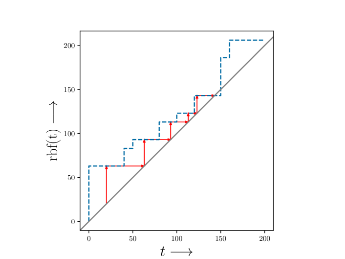
Figure 1. $\operatorname{rbf}(t)$ (blue, dashed) for the system in Table 1 and progress of RTA (red, solid arrows) from initial value $20$ (upward arrows denote the computation of $\operatorname{rbf}(\underline{t})$ and the rightward arrows denote the update $\underline{t}\leftarrow\operatorname{rbf}(\underline{t})$.).

2.2. EDF schedulability and QPA

We limit ourselves to arbitrary-deadline preemptive uniprocessor EDF systems, and simply call them EDF systems. We assume that tasks are listed in nondecreasing order of $\hat{D}_{i}-T_{i}$ in EDF systems, where

$$\hat{D}_{i}=D_{i}-J_{i}$$

An EDF system is unschedulable if and only if $\sum_{j\in[n]}U_{j}>1$ or

$$\exists t\in\rinterval{\hat{D}_{\min}}{L}:t<\operatorname{dbf}(t),$$ (4)

holds (Baruah et al., 1990b; Ripoll et al., 1996; Spuri, 1996a; Zhang and Burns, 2013). Here, $\operatorname{dbf}$, the demand bound function of the system $[n]$, is given by

$$t\mapsto\sum_{j\in[n],t\geq\hat{D}_{j}-T_{j}}\left\lfloor\frac{t+T_{j}-\hat{D}_{j}}{T_{j}}\right\rfloor C_{j},$$ (5)

and $L$ is a large constant like $\operatorname{lcm}_{j}T_{j}$ (more details on $L$ will be provided shortly).

The above condition is satisfied if and only if the problem

$$\max\{t\in\rinterval{\hat{D}_{\min}}{L}\cap\mathbb{Z}:t<\operatorname{dbf}(t)\}$$ (6)

has an optimal solution. It can be shown that the optimal solution $t^{*}$, if it exists and is not trivially equal to $L-1$, is the largest $t\in\rinterval{\hat{D}_{\min}}{L}$ that satisfies

$$\operatorname{dbf}(t)-1=t,$$

i.e., $t^{*}$ is the largest fixed point of $\operatorname{dbf}(\cdot)-1$. $t^{*}$ can be found by starting a safe upper bound $\overline{t}$ for the fixed point and iteratively updating $\overline{t}$ to $\operatorname{dbf}(\overline{t})-1$. This algorithm is called QPA. The inventors of QPA use a slightly more elaborate iterative step (Zhang and Burns, 2013, Alg. 2), but the above update works assuming that all data are integral. Theorem 3.1 can be applied to derive the following theorem; see the discussion preceding Theorem 5.1.

Theorem 2.2.

Problem (6) can be solved by QPA in

$$\mathcal{O}\left(\frac{(L-\hat{D}_{\min})n^{2}}{T_{\mathrm{hm}}}\right)$$

running time.

Some similarities and differences between RTA and QPA are summarized in Table 2.

	RTA	QPA
system	synchronous, preemptive, uniprocessor, constrained-deadline, FP	synchronous, preemptive, uniprocessor, arbitrary-deadline, EDF
iteration	update $t$ to $\operatorname{rbf}(t)$	update $t$ to $\operatorname{dbf}(t)-1$
final value	least fixed point of $\operatorname{rbf}(\cdot)$, if system is schedulable	greatest fixed point of $\operatorname{dbf}(\cdot)-1$, if system is unschedulable

Table 2. Comparing RTA and QPA.

2.3. The upper bound $L$

The interval of interest in Problem (6) is $\rinterval{\hat{D}_{\min}}{L}$. The hyper-period of the system, denoted $\mathcal{T}$, equals $\operatorname{lcm}\{T_{i}\mid i\in[n]\}$ and can be used as $L$. A stronger bound

$$L_{a}=\min\{t\in\linterval{0}{\mathcal{T}}\mid\,\operatorname{rbf}(t)\leq t\}.$$ (7)

can be used as $L$ but it is harder to compute than the hyper-period. Finally, if $\sum_{j\in[n]}U_{j}<1$, then

$$L_{b}=\max\left\{\max_{j\in[n]}\{\hat{D}_{j}-T_{j}\},\frac{\sum_{j\in[n]}(T_{j}-\hat{D}_{j})U_{j}}{1-\sum_{j\in[n]}U_{j}}\right\}$$ (8)

can also be used as $L$. Many researchers have contributed to these bounds; more details are provided, for instance, by George et al. (1996) and Zhang and Burns (2013).

3. Background

3.1. Fixed-point iteration

A fixed point of a function $f$ is a point $x$ such that

$$f(x)=x$$

Given an initial approximation $x_{0}$ of a fixed point of $f$, fixed-point iteration involves repeatedly applying $f$ to generate the sequence:

$$f(x_{0}),f(f(x_{0})),f(f(f(x_{0}))),\dotsc$$

In numerical analysis, the function is often a continuous real-valued function, and the iteration is terminated when the last two generated values are within some tolerance (see, for instance, Burden and Faires, 2011, pg. 60). We will use fixed-point iteration only for monotonic step functions with a finite number of steps in any bounded interval. For such functions, fixed-point iteration can be shown to have the following property.

Theorem 3.1.

(Sjodin and Hansson, 1998, Thm. 1) Let $\interval{a}{b}$ be an interval and let $f$ be a monotonically nondecreasing step function on $\interval{a}{b}$ with at most $n$ steps. One of the following statements must be true:

1. $f(a)\leq a$.

2. Fixed-point iteration with initial value $a$ terminates in at most $n$ steps; if fixed points of $f$ lie in $\interval{a}{b}$, then the iteration converges to the smallest fixed point in $\interval{a}{b}$, otherwise a value larger than $b$ is generated.

Although the above theorem was originally proved in the context of RTA (see Section 2.1), it also works more generally.

3.2. Integer programs

An optimization problem on the variable $x$ that can be expressed as

$$\min\{c\cdot x\mid x\in\mathbb{R}^{n}_{\geq 0},Ax\geq b\},$$ (9)

for some $m\times n$ matrix $A\in\mathbb{R}^{m\times n}$, $b\in\mathbb{R}^{m}$, $c\in\mathbb{R}^{n}$ is a linear program. Here $c\cdot x$ is the dot product of the vectors. LPs can be solved using methods such as the Fourier-Motzkin elimination method, the simplex method (Dantzig, 1987), the ellipsoid method (Khachiyan, 1980), and interior point methods (Karmarkar, 1984). The last two methods are known to run in polynomial time, and thus have theoretical significance.

If $x$ is restricted to be integral, then the problem is an integer program (IP):

$$\min\{c\cdot x\mid x\in\mathbb{Z}^{n}_{\geq 0},Ax\geq b\}.$$ (10)

A relaxation of an optimization problem with a maximization (resp., minimization) objective is a simpler optimization problem with optimal value at least as large (resp., small) as the optimal value of the original problem. Problems can be relaxed in many ways, but we will primarily be concerned with relaxations of integer programs where the set of feasible solutions is expanded by

• allowing variables to be continuous instead of integral; and/or

• dropping constraints.

If the relaxation only involves making the variables continuous, then it is called a linear relaxation. Thus, program (9) is a linear relaxation of program (10).

3.3. Cutting-plane methods

IPs can be solved using the cutting-plane methodology, which consists of repeating the following steps:

1. Solve a relaxation of the IP; usually, the linear relaxation of the IP is chosen.

2. If the relaxation is found to be infeasible, then the IP is infeasible and we return “infeasible”.

3. If the optimal solution for the relaxation is integral, then it is an optimal solution for the IP, and we return the solution.

4. If the optimal solution for the relaxation is not integral, then find one or more cuts or valid inequalities that hold for all points in the convex hull of the set of feasible solutions for the IP but do not hold for the current solution. Since the cut separates the current solution from the feasible solutions, the problem of finding cuts is called the separation problem.

5. Add the cuts to the IP and go to the first step.

After each iteration, we have a better approximation for the convex hull of the set of feasible solutions for the IP, but the problem description, in general, is longer. Since the problem is more restricted in each iteration, the optimal values for the relaxations generated in successive iterations of the cutting-plane algorithm, denoted $\underline{Z}_{1},\underline{Z}_{2},\dotsc$, must satisfy

$$\underline{Z}_{1}\leq\underline{Z}_{2}\leq\dotsb$$

assuming that the direction of optimization is minimization. These values are sometimes called dual bounds for the optimal value for the IP. More details about integer programs can be found in standard textbooks (Wolsey, 1998).

3.4. Linear programming duality

The linear program

$$\max\{b\cdot y\mid y\in\mathbb{R}^{m}_{\geq 0},A^{T}y\leq c\}$$ (11)

is called the dual of LP (9); LP (9) is called the primal program in such a context. Linear programming duality is the idea that for such a pair of programs exactly one of the following statements is true:

• Both programs are infeasible.

• One program is unbounded, and the other program is infeasible.

• Both programs have optimal solutions with the same objective value.

The two programs have optimal solutions $x^{*}$ and $y^{*}$ with the same objective value if and only if they satisfy complementary slackness conditions:

• For all $i\in[m]$, $x^{*}$ satisfies the $i$-th constraint of LP (9) with equality or $y^{*}_{i}=0$.

• Similarly, for all $i\in[n]$, $y^{*}$ satisfies the $i$-th constraint of LP (11) with equality or $x^{*}_{i}=0$.

More details about linear programming duality can be found in standard textbooks (Matoušek and Gärtner, 2007).

4. Integer programs for FP and EDF schedulability

Here, we consider IP formulations for Problem (3) and Problem (6); recall from Section 2 that these problems are essentially equivalent to the FP and EDF schedulability problems.

4.1. IP-FP

Consider the following IP:

$$\begin{array}[]{rrclcl}\min&\lx@intercol t\hfil\lx@intercol\\ \textrm{s.t.}&t&\geq&1\\ &t&\leq&D_{n}-J_{n}\\ &t-\sum_{j\in[n]}C_{j}x_{j}&\geq&0\\ &T_{i}x_{i}-t&\geq&J_{i},&&i\in[n]\\ &t&\in&\mathbb{Z}\\ &x&\in&\mathbb{Z}^{n}\end{array}$$

We show that this IP is equivalent to Problem (3) in the next theorem, and we call it IP-FP.

Theorem 4.1.

Problem (3) has a solution $t^{*}$ if and only if IP-FP has a solution $(t^{*},x^{*})$ for some $x^{*}\in\mathbb{Z}^{n}$.

Proof Sketch.

Any optimal solution $(t^{*},x^{*})$ to the IP satisfies the following identities:

$$t^{*} =\max\left\{\sum_{j\in[n]}C_{j}x^{*}_{j},1\right\}$$

$$x^{*}_{i} =\Bigg{\lceil}\frac{t^{*}+J_{i}}{T_{i}}\Bigg{\rceil},\quad i\in[n]$$

Since $t^{*}\geq 1$ and $J_{i}\geq 0$, $x^{*}_{i}\geq 1$. Then, using the first identity and the fact that $C_{i}>0$ for all $i$, we have $t^{*}\geq\sum_{j\in[n]}C_{j}>1$. Then, the first identity can be simplified to

$$t^{*}=\sum_{j\in[n]}C_{j}x^{*}_{j}=\sum_{j\in[n]}\Bigg{\lceil}\frac{t^{*}+J_{j}}{T_{j}}\Bigg{\rceil}C_{j}=\operatorname{rbf}(t^{*})$$

The third equality uses the definition of $\operatorname{rbf}$ (Definition (2)). Since the objective is to minimize $t$, $t^{*}$ is the smallest $t$ in $\linterval{0}{D_{n}-J_{n}}$ satisfying $t=\operatorname{rbf}(t)$. Thus, $t^{*}$ is a solution for Problem (3). ∎

Similar IP or MILP (mixed-integer linear programming) formulations may be found in the literature (see, for instance, Baruah and Fisher, 2005; Zeng and Di Natale, 2013). In most cases in the literature, new methods for solving the formulations are not proposed: the use of IP/MILP solvers or generic methods such as branch-and-bound for solving IPs is implicitly suggested. We will propose a new cutting-plane algorithm for solving IP-FP in Section 5.3. Zeng and Di Natale (2013) claim that since their formulation contains $\mathcal{O}(n^{2})$ variables “solving the MILP problem in feasible time is impossible for medium and sometimes small size systems.” This claim, however, seems to be based on intuition rather than evidence. Their formulation can be trivially decomposed into $n$ IPs each containing $\mathcal{O}(n)$ variables and constraints, and we will show soon that our cutting-plane algorithm can solve IP-FP in fewer iterations than RTA uses to solve the corresponding instance of Problem (3).

4.2. IP-EDF

The EDF schedulability condition is more complex than the FP schedulability condition, and the process of formulating it as an integer program is error-prone (see discussion in Appendix C). Instead of trying to formulate the EDF schedulability condition as a single IP, we divide it into $\mathcal{O}(n)$ subproblems with simple IP formulations. Recall our assumption that in EDF systems tasks are listed in a nondecreasing order using the key $\hat{D}_{j}-T_{j}$ for each task $j$. Now, we consider the following $n$ subintervals of $\rinterval{\hat{D}_{\min}}{L}$:

$$\rinterval{\hat{D}_{1}-T_{1}}{\hat{D}_{2}-T_{2}}\cap\rinterval{\hat{D}_{\min}}{L},$$

$$\rinterval{\hat{D}_{2}-T_{2}}{\hat{D}_{3}-T_{3}}\cap\rinterval{\hat{D}_{\min}}{L},$$

$$\dotsc,$$

$$\rinterval{\hat{D}_{n-1}-T_{n-1}}{\hat{D}_{n}-T_{n}}\cap\rinterval{\hat{D}_{\min}}{L},$$

$$\rinterval{\hat{D}_{n}-T_{n}}{L}\cap\rinterval{\hat{D}_{\min}}{L}.$$

We ignore $\rinterval{\hat{D}_{\min}}{\hat{D}_{1}-T_{1}}$ because for any $m$ such that $\hat{D}_{m}=\hat{D}_{\min}$, we must have

$$\hat{D}_{1}-T_{1}\leq\hat{D}_{m}-T_{m}<D_{m}=\hat{D}_{\min},$$

and thus the interval is empty. Thus, the family of subintervals is a partition of $\rinterval{\hat{D}_{\min}}{L}$.

Some or all of the intervals considered in the above list may be empty; for instance, only the last interval is nonempty in a constrained-deadline system. Thus, in the $n$ intervals listed above, we can restrict our attention from the $p$-th interval to the $q$-th interval, where

$$p =\min\{i\in[n]\mid i==n\lor\hat{D}_{i+1}-T_{i+1}\geq\hat{D}_{\min}\}$$

$$q =\max\{i\in[n]\mid\hat{D}_{i}-T_{i}<L\}$$

For any $k\in[q]\setminus[p-1]$, let $\rinterval{a_{k}}{b_{k}}$ refer to the $k$-th interval. The $\operatorname{dbf}$ function in $\rinterval{a_{k}}{b_{k}}$ can be simplified to a simpler function $\operatorname{dbf}_{k}$ given by

$$t\mapsto\sum_{i\in[k]}\left\lfloor\frac{t+T_{i}-\hat{D}_{i}}{T_{i}}\right\rfloor C_{i}$$

because

$$t<b_{k}\leq\hat{D}_{k+1}-T_{k+1}\leq\hat{D}_{k+2}-T_{k+2}\leq\dotsb\leq L.$$

Using $\operatorname{dbf}_{k}$, the EDF unschedulability condition (see Condition (4)) can be rewritten as follows: an EDF system is unschedulable if and only if $\sum_{j\in[n]}U_{j}>1$ or there exists a $k\in[n]$ such that

$$\exists t\in\rinterval{a_{k}}{b_{k}}:t<\operatorname{dbf}_{k}(t)$$ (12)

By replacing $t$ with $-t$, Condition (12) can be rewritten as

$$\exists t\in\linterval{-b_{k}}{-a_{k}}:t+\operatorname{dbf}_{k}(-t)\geq 1$$

Using the identity $\lfloor-x\rfloor=-\lceil x\rceil$, we have

$$\operatorname{dbf}_{k}(-t) =\sum_{i\in[k]}\left\lfloor\frac{-t+T_{i}-\hat{D}_{i}}{T_{i}}\right\rfloor C_{i}$$

$$=-\sum_{i\in[k]}\left\lceil\frac{t+\hat{D}_{i}-T_{i}}{T_{i}}\right\rceil C_{i}.$$

Thus, the condition can be rewritten again as

$$\exists t\in\linterval{-b_{k}}{-a_{k}}:\sum_{i\in[k]}\left\lceil\frac{t+\hat{D}_{i}-T_{i}}{T_{i}}\right\rceil C_{i}+1\leq t.$$ (13)

Condition (13) is satisfied if and only if the problem

$$\min\left\{t\in\linterval{-b_{k}}{-a_{k}}\cap\mathbb{Z}\mathrel{\Bigg{|}}\sum_{i\in[k]}\left\lceil\frac{t+\hat{D}_{i}-T_{i}}{T_{i}}\right\rceil C_{i}+1\leq t\right\}$$ (14)

has an optimal solution. The above analysis is distilled into Algorithm 1.

Algorithm 1 Solve EDF schedulability by branching.

1:Sort tasks in a nondecreasing order using the key $i\mapsto\hat{D}_{i}-T_{i}$.

2:if $\hat{D}_{\min}\geq L$ then

3:     return “infeasible”

4:end if

5:$p\leftarrow 1$

6:while $p\leq n-1$ do

7:     if $\hat{D}_{p+1}-T_{p+1}\geq\hat{D}_{\min}$ then

8:         break

9:     end if

10:     $p\leftarrow p+1$

11:end while

12:$q\leftarrow n$

13:while $q\geq 1$ do

14:     if $\hat{D}_{q}-T_{q}<L$ then

15:         break

16:     end if

17:     $q\leftarrow q-1$

18:end while

19:$k\leftarrow q$

20:while $k\geq p$ do

21:     $a_{k}\leftarrow\max(\hat{D}_{\min},\hat{D}_{k}-T_{k})$

22:     if $k=n$ then

23:         $b_{k}\leftarrow L$

24:     else

25:         $b_{k}\leftarrow\hat{D}_{k+1}-T_{k+1}$

26:     end if

27:     Solve problem (14).

28:     if an optimal solution exists then

29:         return the negation of optimal value

30:     end if

31:     $k\leftarrow k-1$

32:end while

33:return “infeasible”

Since Problem (14) is very similar to Problem (3), it can be formulated as an IP similar to IP-FP:

$$\begin{array}[]{rrclcl}\min&\lx@intercol t\hfil\lx@intercol\\ \textrm{s.t.}&t&\geq&-b_{k}+1\\ &t&\leq&-a_{k}\\ &t-\sum_{j\in[k]}C_{j}x_{j}&\geq&1\\ &T_{i}x_{i}-t&\geq&\hat{D}_{i}-T_{i},&&i\in[k]\\ &t&\in&\mathbb{Z}\\ &x&\in&\mathbb{Z}^{k}\end{array}$$

This IP is equivalent to Problem (14), and we call it IP-EDF. We omit the proof because it is the same as the proof for Theorem 4.1.

Theorem 4.2.

Problem (14) has a solution $t^{*}$ if and only if IP-EDF has an optimal solution $(t^{*},x^{*})$ for some $x^{*}\in\mathbb{Z}^{k}$.

Thus, EDF schedulability can be solved by combining Algorithm 1 and some method for solving IP-EDF. We demonstrate the process through an example.

Example 2.

The EDF system in the Table 3 misses a deadline at time $10$. The tasks are sorted in a nondecreasing order using the key $i\mapsto\hat{D}_{i}-T_{i}$. $\hat{D}_{\min}$ and $L$ equal $10$ and $13$ respectively.

$i$	$C_{i}$	$D_{i}$	$T_{i}$
$1$	$6$	$10$	$17$
$2$	$5$	$10$	$13$
$3$	$1$	$31$	$20$

Table 3. An EDF task system with arbitrary deadlines and zero release jitter.

Running Algorithm 1 on the system, we find that the condition on line 2 is not satisfied. The calculation on lines 5–18 yields $p=2$ and $q=3$. In the loop, we solve Problem (14) for $(a_{3},b_{3})=(11,13)$ and $(a_{2},b_{2})=(10,11)$ in order. In the former case, we do not find a feasible solution; in the latter case, we get the following IP:

$$\begin{array}[]{rrclcl}\min&\lx@intercol t\hfil\lx@intercol\\ \textrm{s.t.}&t&\geq&-10\\ &t&\leq&-10\\ &t-6x_{1}-5x_{2}&\geq&1\\ &17x_{1}-t&\geq&-7\\ &13x_{2}-t&\geq&-3\\ &t,x_{1},x_{2}&\in&\mathbb{Z}\end{array}$$

$(t,x_{1},x_{2})=(-10,-1,-1)$ is an optimal solution for the IP, and hence the system is unschedulable.

5. The Kernel

The following problem is called the kernel:

$$\min\left\{t\in\interval{a}{b}\cap\mathbb{Z}\mathrel{\Bigg{|}}\sum_{j\in[n]}\Bigg{\lceil}\frac{t+\alpha_{j}}{T_{j}}\Bigg{\rceil}C_{j}+\beta\leq t\right\},$$ (15)

where

• $n$ is a nonnegative integer.

• For any $i\in[n]$, $C_{i},T_{i}\in\mathbb{Z}_{>0}$ are constants, and $U_{i}$ denotes the ratio $C_{i}/T_{i}$. We assume that $\sum_{j\in[n]}U_{j}\leq 1$.

• $\alpha\in\mathbb{Z}^{n}$, $\beta\in\mathbb{Z}$, $a\in\mathbb{Z}$, and $b\in\mathbb{Z}$ are constants.

It may be useful to view $C_{i}$, $T_{i}$, and $U_{i}$ as the wcet, period, and utilization, respectively, of task $i$; on the other hand, this interpretation can be ignored and $C$, $T$, and $U$ may be viewed simply as vectors of dimension $n$ that satisfy the above properties.

If $(n,\alpha,\beta,a,b)$ is equal to $(n,J,0,1,D_{n}-J_{n})$, then the kernel is identical to Problem (3). If $(n,\alpha,\beta,a,b)$ is equal to $(k,\hat{D}-T,1,-b_{k}+1,-a_{k})$, then the kernel is identical to Problem (14). Thus, the FP and EDF schedulability problems reduce to the kernel. If $(n,\alpha,\beta,a,b)$ is equal to $(n,J,0,1,\mathcal{T})$, then the kernel is identical to the problem of computing $L_{a}$ (see Definition 7). In the next subsections, we will propose two algorithms to solve the kernel, FP-KERN and CP-KERN.

5.1. FP-KERN

If an optimal solution $t^{*}$ for the kernel exists and does not trivially equal $a$, then $t^{*}$ is the smallest $t\in\interval{a}{b}$ that satisfies

$$\sum_{j\in[n]}\Bigg{\lceil}\frac{t+\alpha_{j}}{T_{j}}\Bigg{\rceil}C_{j}+\beta=t;$$

equivalently, $t^{*}$ is the smallest fixed point of $\phi$ in $\interval{a}{b}$ where $\phi$ is given by

$$t\mapsto\sum_{j\in[n]}\Bigg{\lceil}\frac{t+\alpha_{j}}{T_{j}}\Bigg{\rceil}C_{j}+\beta.$$

Since $\phi$ is a monotonically nondecreasing step function. The number of steps in $\interval{a}{b}$ is roughly equal to

$$\sum_{j\in[n]}\frac{b-a}{T_{i}}=\frac{(b-a)n}{T_{\mathrm{hm}}}$$

From Theorem 3.1, $t^{*}$ can be found by fixed-point iteration in no more than $n(b-a)/T_{\mathrm{hm}}$ steps. Since each iteration requires $\mathcal{O}(n)$ arithmetic operations, the algorithm requires $\mathcal{O}((b-a)n^{2}/T_{\mathrm{hm}})$ time. The fixed-point iteration algorithm is called FP-KERN and is listed as Algorithm 2.

Algorithm 2 FP-KERN, a fixed-point iteration algorithm for the kernel.

1:if $a>b$ then

2:     return “infeasible”

3:end if

4:if $n=0$ then

5:     return $a$

6:end if

7:Initialize $\underline{t}$ to $a$.

8:repeat

9:     $v\leftarrow\phi(\underline{t})$

10:     if $v\leq\underline{t}$ then

11:         return $\underline{t}$

12:     end if

13:     $\underline{t}\leftarrow v$

14:until $\underline{t}>b$

15:return “infeasible”

Theorem 5.1.

FP-KERN (Algorithm 2) is a fixed-point iteration algorithm for the kernel with

$$\mathcal{O}\left(\frac{(b-a)n^{2}}{T_{\mathrm{hm}}}\right)$$

running time.

5.2. IP-KERN

Consider the following IP:

$$\begin{array}[]{rrclcl}\min&\lx@intercol t\hfil\lx@intercol\\ \textrm{s.t.}&t&\geq&a\\ &t&\leq&b\\ &t-\sum_{j\in[n]}C_{j}x_{j}&\geq&\beta\\ &T_{i}x_{i}-t&\geq&\alpha_{i},&&i\in[n]\\ &t&\in&\mathbb{Z}\\ &x&\in&\mathbb{Z}^{n}\end{array}$$ (16)

We can compose this IP with the reductions discussed near the start of Section 5 to get IP-FP and IP-EDF. The proof for the validity of the formulation IP-FP (Theorem 4.1) can be trivially modified to show that IP (16) is valid for the kernel. Although IP (16) is a perfectly good formulation, we also include lower bounds for $x$ in our final IP formulation for the kernel. From $t\geq a$ and the fourth constraint in IP (16), we can infer that

$$x_{i}\geq\frac{a+\alpha_{i}}{T_{i}},\quad i\in[n].$$

Since $x_{i}$ is integral, we can infer stronger lower bounds:

$$x_{i}\geq\Bigg{\lceil}\frac{a+\alpha_{i}}{T_{i}}\Bigg{\rceil},\quad i\in[n].$$

Adding these lower bounds to the IP, we have our final IP formulation for the kernel, which we call IP-KERN:

$$\begin{array}[]{rrclcl}\min&\lx@intercol t\hfil\lx@intercol\\ \textrm{s.t.}&t&\geq&a\\ &t&\leq&b\\ &t-\sum_{j\in[n]}C_{j}x_{j}&\geq&\beta\\ &T_{i}x_{i}-t&\geq&\alpha_{i},&&i\in[n]\\ &x_{i}&\geq&\underline{x}_{i},&&i\in[n]\\ &t&\in&\mathbb{Z}\\ &x&\in&\mathbb{Z}^{n}\end{array}$$ (17)

Here, $\underline{x}_{i}$ is a lower bound for $x_{i}$ given by

$$\underline{x}_{i}=\lceil(a+\alpha_{i})/T_{i}\rceil.$$ (18)

This equation holds initially but $\underline{x}$ is repeatedly updated to larger integral vectors in the cutting-plane algorithm described in the next section. The next theorem follows from the above discussion.

Theorem 5.2.

The kernel has a solution $t^{*}$ if and only if IP-KERN has an optimal solution $(t^{*},x^{*})$ for some $x^{*}\in\mathbb{Z}^{k}$.

5.3. A cutting-plane algorithm for IP-KERN

5.3.1. The relaxation

When solving an IP using cutting planes, we must solve a relaxation of the IP. Usually, a linear relaxation is used, but we will also drop the upper and lower bounds on $t$ in our relaxation.

$$\begin{array}[]{rrclcl}\min&\lx@intercol t\hfil\lx@intercol\\ \textrm{s.t.}&t-\sum_{j\in[n]}C_{j}x_{j}&\geq&\beta\\ &T_{i}x_{i}-t&\geq&\alpha_{i},&&i\in[n]\\ &x_{i}&\geq&\underline{x}_{i},&&i\in[n]\\ &t&\in&\mathbb{R}\\ &x&\in&\mathbb{R}^{n}\end{array}$$ (19)

Let $t^{*}$ denote the optimal value of this relaxation. Since the objective is to minimize $t$, if the optimal value of the relaxation is greater than $b$, then the proper linear relaxation of IP-KERN is infeasible, and hence IP-KERN is also infeasible (see Section 3.3). Thus, if $t^{*}>b$, then we can terminate the algorithm, returning “infeasible”. To understand why $t^{*}\geq a$ is dropped from the IP, note that

$$t^{*} \geq\sum_{j\in[n]}C_{j}x_{j}+\beta$$ (using the first constraint in the LP)

$$\geq\sum_{j\in[n]}C_{j}\underline{x}_{j}+\beta$$ (using the third constraint in the LP)

$$\geq\sum_{j\in[n]}C_{j}\lceil(a+\alpha_{j})/T_{j}\rceil+\beta$$ (using Equation 18)

Thus, if $t^{*}\leq a$ then we must have

$$\sum_{j\in[n]}C_{j}\lceil(a+\alpha_{j})/T_{j}\rceil+\beta\leq a$$

which implies that $t=a,x_{j}=\lceil(a+\alpha_{j})/T_{j}\rceil$ is a feasible, and hence optimal, solution to IP-KERN. Thus, if $t^{*}\leq a$, then we can terminate the algorithm returning $a$.

We will see shortly that the form of this LP remains constant for the entire execution of the cutting-plane algorithm: only $\underline{x}$ is updated to a larger integral vector in each iteration.

5.3.2. The separation problem

Solving the separation problem is an essential step in any cutting-plane algorithm. Let us assume that $(t^{*},x^{*})$ is an optimal solution for the relaxation, $(t^{**},x^{**})$ is an optimal solution for the IP, and $(t,x)$ is a feasible solution for the IP. Then, $(t^{*},x^{*})$ must satisfy the following equations:

$$t^{*} =\textstyle\sum_{j\in[n]}C_{j}x^{*}_{j}$$

$$x^{*}_{i} =\max\left\{\frac{t^{*}+\alpha_{i}}{T_{i}},\underline{x}_{i}\right\},\quad i\in[n]$$

If $x^{*}$ is integral, then $t^{*}$ is also integral, and we have found an optimal solution to IP-KERN. Otherwise, there must exist a $j\in[n]$ such that $x^{*}_{j}$ is fractional. $x^{*}_{j}$ cannot equal $\underline{x}_{j}$, which is integral; therefore, it must equal $(t^{*}+\alpha_{j})/T_{j}$. Since $t^{*}$ is a dual bound for the IP and the objective is to minimize $t$, we must have

$$t\geq t^{**}\geq t^{*}.$$

Then, using the fourth constraint in the IP, $(t,x)$ must satisfy

$$x_{j}\geq\frac{t+\alpha_{j}}{T_{j}}\geq\frac{t^{*}+\alpha_{j}}{T_{j}}=x^{*}_{j}.$$

Since $x_{j}$ is integral, the stronger inequality

$$x_{j}\geq\lceil x^{*}_{j}\rceil$$

is also valid. Since $x^{*}_{j}$ is fractional, $x_{j}^{*}\geq\lceil x^{*}_{j}\rceil$ does not hold. Thus, the inequality $x_{j}\geq\lceil x^{*}_{j}\rceil$ separates the current solution $(t^{*},x^{*})$ from the convex hull of feasible solutions and is a cut (see Section 3.3). For each fractional element in $x^{*}_{j}$, a cut is added to the IP by updating the lower bound $\underline{x}_{j}$:

$$\underline{x}_{j}\leftarrow\lceil x^{*}_{j}\rceil.$$

This step requires $\mathcal{O}(n)$ arithmetic operations, it does not change the number of variables or the number of constraints in the IP, and it maintains the integrality of $\underline{x}$, which is utilized in generating cuts in the next iteration.

Note that we could have used general cuts like Gomory cuts (see, for instance, Wolsey, 1998, Ch. 8.6) in our cutting-plane algorithm but we choose to use a cut generation technique that is specialized for our problem. While we do not claim to generate the strongest cuts, our cuts have nice properties: they are generated efficiently and do not change the number of variables and number of constraints in the IP. Moreover, we will show in the next section that FP-KERN is also a cutting-plane algorithm with the same cut generation technique but a different relaxation.

The cutting-plane algorithm that we have developed in this section is called CP-KERN and is listed as Algorithm 3. For any $i\in[n]$, the minimum (resp., maximum) value of $\underline{x}_{i}$ is $\lceil(a+\alpha_{i})/T_{i}\rceil$ (resp., $\lceil(b+\alpha_{i})/T_{i}\rceil$); thus, $\underline{x}_{i}$ can assume $\mathcal{O}((b-a)/T_{i})$ values. Since at least one element in $\underline{x}$ is incremented in each iteration, the maximum number of iterations is roughly equal to

$$\sum_{j\in[n]}\frac{b-a}{T_{i}}=\frac{(b-a)n}{T_{\mathrm{hm}}}$$

In each iteration, the linear program can be solved in time polynomial in the size of the representation of the program (Khachiyan, 1980). The size of the representation of the program is linearly bounded by the size of the representation of the original instance of the kernel, denoted $\lvert I\rvert$. Thus, the algorithm has $\mathcal{O}((b-a)\mathsf{poly}(\lvert I\rvert)/T_{\mathrm{hm}})$ running time.

Algorithm 3 CP-KERN, a cutting-plane algorithm for the kernel.

1:if $a>b$ then

2:     return “infeasible”

3:end if

4:if $n=0$ then

5:     return $a$

6:end if

7: Initialize $\underline{x}_{i}=\lceil(a+\alpha_{i})/T_{i}\rceil$ for all $i\in[n]$.

8:repeat

9:      Solve LP (19). If infeasible, return “infeasible”, else let $(t^{*},x^{*})$ be the optimal solution.

10:     if $t^{*}\leq a$ then

11:         return $a$

12:     end if

13:     if $t^{*}>b$ then

14:         return “infeasible”

15:     end if

16:      Update $\underline{x}_{i}$ to $\lceil x^{*}_{i}\rceil$ for all $i\in[n]$.

17:until $\underline{x}$ stabilizes.

18:return $C\cdot\underline{x}+\beta$

Theorem 5.3.

CP-KERN (Algorithm 3) is a cutting-plane algorithm for the kernel with

$$\mathcal{O}\left(\frac{(b-a)\mathsf{poly}(\lvert I\rvert)}{T_{\mathrm{hm}}}\right)$$

running time.

Example 2 (contd.).

We will solve the schedulability problem for the lowest priority task in the FP task system in Table 1 by reducing it to the kernel, formulating the kernel as IP-KERN, and solving IP-KERN by using CP-KERN. The kernel is given by

$$\min\left\{t\in\interval{1}{D_{3}}\cap\mathbb{Z}\mathrel{\Bigg{|}}\sum_{j\in[3]}\Bigg{\lceil}\frac{t}{T_{i}}\Bigg{\rceil}C_{j}\leq t\right\}.$$

IP-KERN is given by

$$\begin{array}[]{rrclcl}\min&\lx@intercol t\hfil\lx@intercol\\ \textrm{s.t.}&t&\geq&1\\ &t&\leq&150\\ &t-20x_{1}-10x_{2}-33x_{3}&\geq&0\\ &40x_{1}-t&\geq&0\\ &50x_{2}-t&\geq&0\\ &150x_{3}-t&\geq&0\\ &x_{i}&\geq&1,&&i\in[3]\\ &t,x_{1},x_{2},x_{3}&\in&\mathbb{Z}\end{array}$$

We describe the execution of CP-KERN for the above IP. Initially we have $\underline{x}_{i}=1$ for all $i\in[3]$. The relaxation is given by

$$\begin{array}[]{rrclcl}\min&\lx@intercol t\hfil\lx@intercol\\ \textrm{s.t.}&t-20x_{1}-10x_{2}-33x_{3}&\geq&0\\ &40x_{1}-t&\geq&0\\ &50x_{2}-t&\geq&0\\ &150x_{3}-t&\geq&0\\ &x_{i}&\geq&\underline{x}_{i},&&i\in[3]\\ &t,x_{1},x_{2},x_{3}&\in&\mathbb{R}\end{array}$$

We solve the relaxation and get the optimal solution $(t^{*},x^{*})=(110,{2.75,2.2,1})$. We update $\underline{x}$ to $(3,3,1)$. We solve the new relaxation and get $(t^{*},x^{*})=(126,{3.15,3,1})$. We update $\underline{x}$ to $(4,3,1)$. We solve the new relaxation and get $(t^{*},x^{*})=(143,{4,3,1})$. Since $\underline{x}$ has stabilized, we terminate the algorithm. Thus, Algorithm 3 solves the problem in $3$ iterations; recall from Figure 1 that RTA solved the problem in $5$ iterations.

5.4. Comparing FP-KERN and CP-KERN

Let $\mathcal{F}$ denote the family of cutting-plane algorithms for IP KERN where each algorithm satisfies the following properties:

1. In each iteration, the algorithm solves a relaxation of IP-KERN where all integral variables are made continuous and some constraints are dropped optionally.

2. Cuts are generated by rounding up the values of the optimal $x$ values for the relaxation.

Clearly, CP-KERN belongs to $\mathcal{F}$. Although the relaxation used by CP-KERN drops the upper and lower bounds for $t$, these changes are addressed immediately after the relaxation is solved (see discussion near the start of Section 5.3). Thus, CP-KERN effectively solves the proper linear relaxation of IP-KERN, and has the optimal convergence rate in $\mathcal{F}$. We will show that FP-KERN also belongs to $\mathcal{F}$, but it has a suboptimal convergence rate.

Algorithm 2 and Algorithm 4 are equivalent ways to express FP-KERN. While Algorithm 2 uses two variables ($\underline{t},v$), Algorithm 4 uses $n+1$ variables ($\underline{x}_{1},\dotsc,\underline{x}_{n},v$). $v$ is a temporary variable in both cases; $\underline{t}$ and $\underline{x}_{i}$ denote lower bounds for $t$ and $\lceil(t+\alpha_{i})/T_{i}\rceil$ for the kernel. It is easy to see that Algorithm 2 and Algorithm 4 are essentially the same: the computation of $\phi$ in Algorithm 2 is broken into two steps: the ceiling expressions are evaluated at the end of the loop and the resulting values are combined with $C$ and $\beta$ to get $\phi(v)$ at the start of the next loop.

Algorithm 4 An algorithm equivalent to FP-KERN.

1:if $a>b$ then

2:     return “infeasible”

3:end if

4:if $n=0$ then

5:     return $a$

6:end if

7: Initialize $\underline{x}_{i}=\lceil(a+\alpha_{i})/T_{i}\rceil$ for all $i\in[n]$.

8:repeat

9:     $v\leftarrow C\cdot\underline{x}+\beta$

10:     if $v\leq a$ then

11:         return $a$

12:     end if

13:     if $v>b$ then

14:         return “infeasible”

15:     end if

16:      Update $\underline{x}_{i}$ to $\lceil(v+\alpha_{i})/T_{i}\rceil$ for all $i\in[n]$.

17:until $\underline{x}$ stabilizes.

18:return $C\cdot\underline{x}+\beta$

From the description of FP-KERN in Algorithm 4, we can see that FP-KERN is almost the same as CP-KERN except for the fact that the latter solves a relaxation of IP-KERN at the beginning of the loop. It turns out that FP-KERN also solves a relaxation of IP-KERN at the beginning of the loop, and this relaxation has the optimal value $C\cdot\underline{x}+\beta$. The relaxation used by FP-KERN makes all variables continuous and drops the upper and lower bounds of $t$ and the constraint $Tx_{i}-t\geq\alpha_{i}$ for all $i\in[n]$; thus, the relaxation used by FP-KERN is given by

$$\begin{array}[]{rrclcl}\min&\lx@intercol t\hfil\lx@intercol\\ \textrm{s.t.}&t-\sum_{j\in[n]}C_{j}x_{j}&\geq&\beta\\ &x_{i}&\geq&\underline{x}_{i},&&i\in[n]\\ &t&\in&\mathbb{R}\\ &x&\in&\mathbb{R}^{n}\end{array}$$

The optimal value for the relaxation simply equals $C\cdot\underline{x}+\beta$. Since the above relaxation drops more inequalities than the relaxation used by CP-KERN, it does not find the proper dual bounds in each iteration. The suboptimality of FP-KERN is corroborated by the example at the end of Section 5.3 and the empirical evaluations in Section 6.

Theorem 5.4.

CP-KERN (resp., FP-KERN) has an optimal (resp., suboptimal) convergence rate in the family $\mathcal{F}$ of cutting-plane algorithms for solving IP-KERN.

The relaxation used by FP-KERN can be solved in $\Theta(n)$ time since it reduces to evaluating the expression $C\cdot\underline{x}+\beta$. In contrast, the relaxation used by CP-KERN can be solved in $\mathsf{poly}(\lvert I\rvert)$ time by using an algorithm such as the ellipsoid algorithm for solving general LPs. In the next section, we propose a more efficient method for solving the relaxation used by CP-KERN.

5.5. A specialized method for solving the relaxation

In this section, we develop a specialized algorithm for solving the dual of LP (19). Recall from Section 3.4 that solving the dual is effectively the same as solving the relaxation itself, except that the notions of unboundedness and infeasibility are inverted. The dual can be constructed by following a dualization recipe that may be found in any textbook on linear programming (Matoušek and Gärtner, 2007, pg. 85); therefore, we skip the details of the construction. Let $v,w,z$ be the variables in the dual LP such that they correspond, in order, to the three inequalities in the primal LP, i.e., LP (19). Then, the dual is given by:

$$\begin{array}[]{rrclcl}\max&\lx@intercol\beta{}v+\alpha\cdot w+\underline{x}\cdot z\hfil\lx@intercol\\ \textrm{s.t.}&v-\sum_{j\in[n]}w_{j}&=&1\\ &-C_{i}v+T_{i}w_{i}+z_{i}&=&0,&&i\in[n]\\ &v&\in&\mathbb{R}_{\geq 0}\\ &w,z&\in&\mathbb{R}^{n}_{\geq 0}\end{array}$$ (20)

By substituting $z_{i}/T_{i}$ for $z_{i}$ for all $i\in[n]$ and eliminating $w$, we get

$$\begin{array}[]{rrclcl}\max&\lx@intercol(\beta+U\cdot{}\alpha{})v+\sum_{j\in[n]}(T_{j}\underline{x}_{j}-\alpha_{j})z_{j}\hfil\lx@intercol\\ \textrm{s.t.}&(1-\sum_{j\in[n]}U_{j})v+\sum_{j\in[n]}z_{j}&=&1\\ &U_{i}v-z_{i}&\geq&0,&&i\in[n]\\ &v&\in&\mathbb{R}_{\geq 0}\\ &z&\in&\mathbb{R}^{n}_{\geq 0}\end{array}$$ (21)

For a fixed $v$, LP (21) is identical to a fractional knapsack problem with $n$ items where $z_{i}$ is the weight of item $i$ in the knapsack, $U_{i}v$ is the total weight of item $i$ available to the thief, $T_{i}\underline{x}_{i}-\alpha_{i}$ is the value of the item per unit weight, and the knapsack weighs exactly $1-(1-\sum_{j\in[n]}U_{j})v$. The fractional knapsack problem admits a greedy solution in which the thief fills the knapsack with items in nonincreasing order of value until the knapsack is full. By assuming that the vectors $\underline{x}$, $U$, $T$, and $\alpha$ are sorted in nonincreasing order of value, i.e., $T_{i}\underline{x}_{i}-\alpha_{i}$, we can infer that an optimal solution exists such that for some $k\in[n]$,

$$z_{j} =U_{j}v, j\in[k-1]$$

$$z_{k} \leq U_{k}v$$

$$z_{j} =0, j\in[n]\setminus[k]$$

For each $k\in[n]$, we can create a more restricted version of linear program (21) by adding the above constraints:

$$\begin{array}[]{rrclcl}\max&\lx@intercol(\beta+\sum_{j\in[n]\setminus[k-1]}U_{j}\alpha_{j}+\sum_{j\in[k-1]}C_{j}\underline{x}_{j})v+\hfil\lx@intercol\\ &\lx@intercol(T_{k}\underline{x}_{k}-\alpha_{k})z_{k}\hfil\lx@intercol\\ \textrm{s.t.}&(1-\sum_{j\in[n]\setminus[k-1]}U_{j})v+z_{k}&=&1\\ &U_{k}v-z_{k}&\geq&0\\ &v,z_{k}&\in&\mathbb{R}_{\geq 0}\end{array}$$ (22)

The relationship between LP (21) and LP (22) is summarized in the next lemma.

Lemma 5.5.

The following statements are true:

1. LP (21) has an optimal solution $(v,z)$ if and only if for some $k\in[n]$ LP (22) has an optimal solution $(v,z_{k})$.

2. LP (21) is infeasible if and only if LP (22) is infeasible for all $k\in[n]$.

3. LP (21) is unbounded if and only if LP (22) is unbounded for some $k\in[n]$.

In the remainder of this section, we analyze LP (22) under different conditions to find an algorithm for solving LP (21).

Lemma 5.6.

If $\sum_{j\in[n]}U_{j}=1$ and $\beta+U\cdot\alpha>0$, then IP-KERN is infeasible.

Proof Sketch.

Let us assume that $\sum_{j\in[n]}U_{j}=1$ and $\beta+U\cdot\alpha$ is positive. For $k=1$ in LP (22), $v$ disappears from the first constraint and its coefficient in the objective function is positive; thus, the LP is unbounded. Then, using Lemma 5.5, LP (21) is also unbounded. Since LP (19) is a dual of LP (21), it must be infeasible (see Section (3.4)). Since LP (19) is a relaxation of IP-KERN, the infeasibility of the LP implies the infeasibility of IP-KERN. ∎

We introduce a map $f:\{0\}\cup[n]\to\mathbb{Q}$ given by

$$k\mapsto\frac{\beta+\sum_{j\in[n]\setminus[k]}U_{j}\alpha_{j}+\sum_{j\in[k]}C_{j}\underline{x}_{j}}{1-\sum_{j\in[n]\setminus[k]}U_{j}}.$$ (23)

If $k=0$ and $\sum_{j\in[n]}U_{j}=1$, then $f(k)$ is not well-defined; in this case, we restrict the domain of $f$ to $[n]$. The next two lemmas show that optimal values of LP (22) always lie in the image of $f$.

Lemma 5.7.

If $f(0)$ is not well-defined and $\beta+U\cdot\alpha\leq 0$, then the optimal value for LP (22) is $f(1)$.

Proof Sketch.

If $k=1$ and $\sum_{j\in[n]}U_{j}=1$, then it may be verified that the optimal solution is $(v,z_{1})=(1/U_{1},1)$ and the optimal value is

$$(\beta+\sum_{j\in[n]}U_{j}\alpha_{j})(1/U_{1})+(T_{1}\underline{x}_{1}-\alpha_{1})$$

$$= \frac{\beta+\sum_{j\in[n]\setminus[1]}U_{j}\alpha_{j}+C_{1}\underline{x}_{1}}{U_{1}}$$

$$= f(1)$$ (using Definition (23))

∎

Lemma 5.8.

For any $k\in[n]$, if $f(k-1)$ is well-defined, then the optimal value for LP (22) is $f(k)$ or $f(k-1)$.

Proof Sketch.

If $f(k-1)$ is well-defined, then we must have $k>1$ or $\sum_{j\in[n]}U_{j}<1$. Then, $z_{k}$ can be eliminated from LP (22) to get

$$\begin{array}[]{rrclcl}\max&\lx@intercol(1-\sum_{j\in[n]\setminus[k]}U_{j})(f(k)-(T_{k}\underline{x}_{k}-\alpha_{k}))v+T_{k}\underline{x}_{k}-\alpha_{k}\hfil\lx@intercol\\ \textrm{s.t.}&v&\in&\interval{(1-\sum_{j\in[n]\setminus[k]}U_{j})^{-1}}{(1-\sum_{j\in[n]\setminus[k-1]}U_{j})^{-1}}\end{array}$$

From the definition of the kernel, we have $\sum_{j\in[n]}U_{j}\leq 1$. Thus, the left end of the interval is positive, and hence the constraint $v\geq 0$, which was present in program (22), is redundant and is not included above. From the assumption that $k>1$ or $\sum_{j\in[n]}U_{j}<1$, it follows that the right end of the interval is well-defined and greater than the left end of the interval. Thus, program (22) is feasible and bounded. The optimal objective value for the program must be achieved at one of the ends of the interval for $v$, the end being determined by the sign of the coefficient of $v$ in the objective. Using Lemma A.1, the objective can also be written as

$$(1-\textstyle\sum_{j\in[n]\setminus[k-1]}U_{j})(f(k-1)-(T_{k}\underline{x}_{k}-\alpha_{k}))v+T_{k}\underline{x}_{k}-\alpha_{k}.$$

Substituting the two ends of the interval for $v$ in the two expressions for the objective, we get that the optimal value is $f(k)$ or $f(k-1)$. ∎

We accumulate Lemmas 5.6, 5.7, and 5.8 into one theorem:

Theorem 5.9.

If $\sum_{j\in[n]}U_{j}=1$ and $\beta+U\cdot\alpha>0$, then IP-KERN is infeasible; otherwise, LP (19) has optimal value $\max f$ (assuming that all vectors are sorted in a nonincreasing order using the key $T_{j}\underline{x}_{j}-\alpha_{j}$ for each $j\in[n]$).

A detailed version of CP-KERN, with the algorithm for solving the relaxation by computing $\max f$ embedded in it, is listed as Algorithm 5.

Algorithm 5 CP-KERN, detailed

1:if $a>b$ then

2:     return “infeasible”

3:end if

4:if $n=0$ then

5:     return $a$

6:end if

7:$(p,q,r)\leftarrow(\beta,1,\beta)$

8:for all $i\in[n]$ do

9:     $\underline{x}_{i}\leftarrow\lceil(a+\alpha_{i})/T_{i}\rceil$

10:     $y_{i}\leftarrow T_{i}\underline{x}_{i}-\alpha_{i}$

11:     $\pi_{i}\leftarrow i$

12:     $(p,q,r)\leftarrow(p+U_{i}\alpha_{i},q-U_{i},r+C_{i}\underline{x}_{i})$

13:end for

14:if $p>0$ and $q=0$ then

15:     return “infeasible”

16:end if

17:$i_{0}\leftarrow 1$ if $q=0$ else $i_{0}\leftarrow 0$

18: Sort $\pi$ in a nonincreasing order using the key $i\mapsto y_{i}$.

19:while $\top$ do

20:     $(p,q,i)\leftarrow(r,1,n)$

21:     while $i>i_{0}$ do

22:         $k\leftarrow\pi_{i}$

23:         if $p\leq q*y_{k}$ then

24:              $t^{*}\leftarrow p/q$

25:              break

26:         end if

27:         $(p,q,i)\leftarrow(p-C_{k}\underline{x}_{k}+U_{k}\alpha_{k},q-U_{k},i-1)$

28:     end while

29:     if $i=i_{0}$ then

30:         $t^{*}\leftarrow p/q$

31:     end if

32:     if $t^{*}\leq a$ then return $a$; if $t^{*}>b$ then return “infeasible”.

33:     if $i=n$ then

34:         return $t^{*}$

35:     end if

36:     for all $j\in[n]\setminus[i]$ do

37:         $k\leftarrow\pi_{j}$

38:         $d\leftarrow\lceil(t^{*}+\alpha_{k})/T_{k}\rceil-\underline{x}_{k}$

39:         $(\underline{x}_{k},y_{k},r)\leftarrow(\underline{x}_{k}+d,y_{k}+T_{k}d,r+C_{k}d)$

40:     end for

41:      Sort $\pi$ in the range $i+1$ to $n$ in a nonincreasing order using the key $j\mapsto y_{j}$.

42:      Merge the two sorted parts of $\pi$.

43:end while

Theorem 5.10.

CP-KERN (Algorithm 5) solves the kernel in

$$\mathcal{O}\left(\frac{(b-a)n^{2}}{T_{\mathrm{hm}}}\right)$$

running time.

Proof sketch.

Algorithm 5 is essentially the same as Algorithm 3: in each iteration, we solve LP (19) and then update $\underline{x}_{i}$ to $\lceil x^{*}_{i}\rceil$ for all $i\in[n]$. However, there are some differences between the two algorithms:

• We check a new infeasibility condition on line 14. Since $p=\beta+U\cdot\alpha$ and $q=1-\sum_{j\in[n]}U_{j}$ on this line, the condition is equivalent to the infeasibility condition in Theorem 5.9.

• We maintain two vector variables $y$ and $\pi$, where $y_{i}=T_{i}\underline{x}_{i}-\alpha_{i}$ for all $i\in[n]$, and $\pi$ stores the indices of $y$ so that for any $i\leq j$ we have

  $$y_{\pi_{i}}\geq y_{\pi_{j}}.$$

  We also maintain a scalar variable $r=\beta+C\cdot\underline{x}=f(n)$.

• We compute an optimal value $t^{*}$ for LP (19) on lines 20–31. On line 17, $i_{0}$ was set to the smallest point of the domain of $f$. We examine the values in the domain of $f$ excluding the smallest point $i_{0}$ in the inner while loop. On line 23, we have

  $$p/q=f(i)$$

  Thus, in the while loop, we search for an $i$ such that

  $$p/q\leq y_{k}\iff f(i)\leq T_{\pi_{i}}\underline{x}_{\pi_{i}}-\alpha_{\pi_{i}}\iff f(i)\geq f(i-1).$$

  The second equivalence follows from Lemma A.1. Thus, we are looking for a local maximum point of $f$ in its domain (excluding $i_{0}$). Using Corollary A.3, any local maximum point is also a global maximum point. If we do not find any such point, then $i_{0}$ must be a global maximum point of $f$. We store the maximum value of $f$ in the variable $t^{*}$ on lines 24 and 30. If we have reached line 31, then $i$ is a global maximum point of $f$, and it corresponds to a solution for the LP (20) in which

  $$z_{j}>0\land w_{j}=0, j\in\{\pi_{1},\dotsc,\pi_{i}\}$$

  $$z_{j}=0\land w_{j}>0, j\in\{\pi_{i+1},\dotsc,\pi_{n}\}$$

  Using complementary slackness conditions (see Section 3.4), we can infer that in the corresponding solution in LP (19) we must have

  $$x_{j}^{*}=\underline{x}_{j}, j\in\{\pi_{1},\dotsc,\pi_{i}\}$$ (24)

  $$x_{j}^{*}=(t^{*}+\alpha_{j})/T_{j}, j\in\{\pi_{i+1},\dotsc,\pi_{n}\}$$ (25)

  We do not explicitly compute $x^{*}$ in our algorithm, but we use the above equations towards the end of the outer while loop when we update $\underline{x}$.

• Instead of exiting the outer while loop when $\underline{x}$ stabilizes, we exit the loop on line 34 if the condition on line 33 is satisfied. Recall that $i$ is a global maximum point of $f$ after line 31. Thus, the condition on line 33 is equivalent to $n$ being a global maximum point of $f$. From Equation (24), we must have $x_{j}^{*}=\underline{x}_{j}$ for all $j\in[n]$. Furthermore, since the algorithm did not exit on 32, we have

  $$f(n)=t^{*}\in\interval{a}{b}.$$

  Thus, $(t^{*},x^{*})=f(n)$ is an optimal solution for IP-KERN.

• Instead of updating the full vector $\underline{x}$, we do not update the entries corresponding to indices $\{\pi_{1},\dotsc,\pi_{i}\}$ because they are already integral (using Equation (24)). For any other index $j$, $\underline{x}_{j}$ is updated to $\lceil x^{*}_{j}\rceil=\lceil(t^{*}+\alpha_{j})/T_{j}\rceil$ (using Equation (25)). $r$ and $y$ are also modified to reflect the change in $\underline{x}$. Since $\underline{x}_{j}$ is unchanged for all $j\in\{\pi_{1},\dotsc,\pi_{i}\}$, $\pi$ is already sorted in this range. Therefore, we sort $\pi_{i+1},\dotsc,\pi_{n}$, and then we merge the two sorted parts of $\pi$ into one.

Let $n-m_{i}$ be the global maximum point of $f$ in the $i$-th iteration. Then, lines 20–40 run in $\mathcal{O}(m_{i})$ time, and sorting on line 41 takes $\mathcal{O}(m_{i}\log(m_{i}))$ time. Since $m_{i}$ new values of $\underline{x}$ are computed in the loop on line 36 and since each $\underline{x}_{j}$ can assume $\mathcal{O}((b-a)/T_{j})$ values, over all iterations we must have

$$\sum m_{i}=\mathcal{O}\left(\frac{\sum_{j\in[n]}(b-a)}{T_{j}}\right)=\mathcal{O}\left(\frac{(b-a)n}{T_{\mathrm{hm}}}\right)$$

Thus, the time taken by lines 20–41 over all iterations equals

$$\mathcal{O}(\textstyle\sum m_{i}\log(m_{i}))$$

$$= \mathcal{O}(\textstyle\sum m_{i}\log(n)) m_{i}\leq n$$ (since )

$$= \mathcal{O}(\log(n)\textstyle\sum m_{i})$$

$$= \mathcal{O}\left(\frac{(b-a)n\log(n)}{T_{\mathrm{hm}}}\right)$$

In one iteration, line 42 takes $\mathcal{O}(n)$ time. Since our analysis of the number of iterations in Algorithm 3 also applies to the current algorithm, over all iterations line 42 takes

$$\mathcal{O}\left(\frac{(b-a)n^{2}}{T_{\mathrm{hm}}}\right)$$

time. Thus, in our analysis the work done by line 42 dominates the work done by the other lines. We think that the analysis of the number of iterations may be a little pessimistic and deserves further investigation. ∎

5.6. Implications for FP and EDF schedulability

Since Problem (3) can be solved by reducing it to the kernel by setting $(n,\alpha,\beta,a,b)$ to $(n,J,0,1,D_{n}-J_{n})$, the following theorem follows from Theorem 5.10:

Theorem 5.11.

Problem (3) can be solved by CP-KERN in

$$\mathcal{O}\left(\frac{(D_{n}-J_{n})n^{2}}{T_{\mathrm{hm}}}\right)$$

running time.

Since Problem (14) can be solved by reducing it to the kernel by setting $(n,\alpha,\beta,a,b)$ to $(k,D-T-J,1,-b_{k}+1,-a_{k})$, the following theorem follows from Theorem 5.10:

Theorem 5.12.

Problem (14) can be solved by CP-KERN in

$$\mathcal{O}\left(\frac{(b_{k}-a_{k})k^{2}}{T_{\mathrm{hm}}^{k}}\right)$$

running time, where $T_{\mathrm{hm}}^{k}$ is the harmonic mean of the periods $T_{1},\dotsc,T_{k}$.

Since the problem of computing $L_{a}$ (see Definition 7) can be solved by reducing it to the kernel by setting $(n,\alpha,\beta,a,b)$ to $(n,J,0,1,\mathcal{T})$, the following theorem follows from Theorem 5.10:

Theorem 5.13.

$L_{a}$ can be computed by CP-KERN in

$$\mathcal{O}\left(\frac{\mathcal{T}{}n^{2}}{T_{\mathrm{hm}}}\right)$$

running time.

In all cases, the worst-case running times of CP-KERN are the same as the worst-case running times for the corresponding fixed-point iteration algorithms. Since CP-KERN, unlike RTA and QPA, has an optimal convergence rate in the family $\mathcal{F}$ (see Theorem 5.4), CP-KERN is a better algorithm than RTA and QPA in theory.

6. Empirical evaluation

Our goal in this work is not to determine the fastest schedulability test amongst all known tests. As mentioned in the introduction, the schedulability tests are, in general, incomparable and their running times depend on the sizes of parameters like number of periods and $D_{\max}/T_{\min}$. However, the algorithms in the family of cutting-plane algorithms considered in this work are comparable, and we try to quantify the improvement in convergence rate and running time achieved by our optimal cutting-plane algorithm CP-KERN over RTA and QPA for large collections of synthetic systems. In keeping with the aims of the research, we do not include all schedulability tests that exist in literature in our empirical evaluations; instead, we restrict our attention to the family of cutting-plane algorithms studied in this work.

6.1. Environment

We conducted the experiments on a MacBook Pro 2019 with a 2.6 GHz 6-Core Intel Core i7 processor and 16 GB 2400 MHz DDR4 memory.

Our code for carrying out the above experiments is publicly available (Singh, 2023). The code is written in mostly written in Python and it contains

• methods for generating random systems of hard real-time tasks;

• instrumented Python implementations of FP-KERN and CP-KERN that count the number of iterations used by the algorithms;

• instrumented C++ implementations of FP-KERN and CP-KERN that measure the CPU time used by the algorithms;

• reductions from FP and EDF schedulability to the kernel, including the branching approach for EDF described in Algorithm 1 and the optimizations discussed in Appendix B;

• tests for finding inconsistencies between CP-KERN and traditional schedulability tests (RTA and QPA); and

• a script for running the experiments described above and for generating the associated data and images.

We depend on several Python packages including drs, numpy, matplotlib, pytest, and scipy. Our C++ implementation of CP-KERN can produce incorrect answers due to numerical issues stemming from the use of floating-point arithmetic and integer overflow errors. In contrast, our Python implementation of CP-KERN uses rational arithmetic using the fractions module and unlimited-precision integers. Thus, we think that the Python implementation is more trustworthy. In all experiments, we check that the results produced by FP-KERN and CP-KERN are consistent; thus, we have confidence in the validity of the results derived from the C++ implementations.

6.2. Data

In each experiment, we randomly generate $10000$ synthetic task systems. Each system contains $n$ tasks, where $n\in\{25,50,75\}$. We generate utilizations so that their approximate sum is one of the values in $\{0.7,0.8,0.9\}$ by using the Dirichlet-Rescale (DRS) algorithm (Griffin et al., 2020). We sample wcets from a loguniform distribution in $\interval{1}{1000}$, and then round each wcet up to the nearest integer.. We compute period $T_{i}$ as follows:

$$T_{i}\coloneq\Bigg{\lceil}\frac{C_{i}}{U_{i}}\Bigg{\rceil}$$

Since the periods are rounded up, the utilizations are rounded down; thus, the utilization of the system is only approximately equal to our initially chosen value. We generate FP systems and EDF systems differently.

6.2.1. FP systems

We generate FP systems with implicit deadlines and zero release jitter. Thus, we set $D_{i}\coloneq T_{i}$ and $J_{i}\coloneq 0$ for all $i$.

In our current description, the parameter $D_{n}=T_{n}$ is generated just like the other periods $T_{1},\dotsc,T_{n-1}$. However, $D_{n}$ has a disproportionate effect on the running times of algorithms for solving Problem (3). In the current setting, Problem (3) can be written as follows:

$$\min\left\{t\in\linterval{0}{D_{n}}\cap\mathbb{Z}\mathrel{\Bigg{|}}C_{n}+\sum_{j\in[n-1],T_{j}<D_{n}}\left\lceil\frac{t}{T_{j}}\right\rceil{}C_{j}\leq t\right\}$$

Thus, all the periods that are smaller than a randomly generated $D_{n}$ do not contribute to the problem instance. Moreover, since $D_{n}$ is in the numerator in the asymptotic characterization of worst-case running times in Theorems 2.1 and 5.11, a random instance will get solved quickly if $D_{n}$ is small. Therefore, to reduce noise in the evaluation, we set the parameters of task $n$ as follows:

$$D_{n}=T_{n}\coloneq 10^{8},C_{n}\coloneq 100.$$

This ensures that both RTA and CP-KERN are evaluated against challenging instances of Problem (3). The high-priority subsystem $[n-1]$ is generated randomly, as described above.

6.2.2. EDF systems

Recall from Section 4.2 that we use a divide-and-conquer approach to create $n$ subproblems where the $k$-th subproblem is the same as the original problem except that $t$ is restricted to $\interval{a_{k}}{b_{k}}\subseteq\rinterval{\hat{D}_{\min}}{L}$ (see Problem (14)); each subproblem is then reduced to the kernel which is then solved by CP-KERN. The overall algorithm has a branch-and-cut structure where the division into subproblems corresponds to branching on the variable $t$ and using the cutting-plane algorithm CP-KERN corresponds to the finding cuts on the nodes generated from the branching. For constrained-deadline systems, only the branch $\rinterval{\hat{D}_{\min}}{L}$ has feasible solutions. We restrict our attention to constrained-deadline systems in the evaluation so that we do not need to worry about the effect of branching strategies on the results.

We call the ratio $\delta_{i}=C_{i}/D_{i}$ the density of task $i$. We use the DRS algorithm to generate the densities of the tasks so that their approximate sum is one of the values in $\{1.25,1.50,1.75\}$. Since we are generating a constrained-deadline system, we must ensure that the density of any task is at least its utilization; so, we pass the utilization vector to the DRS algorithm as a lower bound for the density vector. We compute the deadline $D_{i}$ as follows:

$$D_{i}\coloneq\Bigg{\lfloor}\frac{C_{i}}{\delta_{i}}\Bigg{\rfloor}.$$

Since deadlines are rounded down, the total density of the system is only approximately equal to the initially chosen value.

6.3. Experiment I

In this experiment, we compare the number of iterations used by RTA to the number of iterations used by CP-KERN for synthetic instances of Problem (3). For both algorithms, we use the initial value

$$\frac{C_{n}}{1-\sum_{j\in[n-1]}U_{j}}.$$

Initial values such as the one mentioned above for RTA have been discussed extensively in the literature (Sjodin and Hansson, 1998; Bril et al., 2003; Davis et al., 2008); in Appendix B, we show that the bound is implicitly used by CP-KERN and can also be explicitly passed to CP-KERN by using an alternative reduction from Problem (3) to the kernel.

For $n=25$ and $\sum_{j\in[n-1]}U_{j}\approx 0.9$, we show histograms of the number of iterations of CP-KERN and RTA in Figure 2(a). The histogram for CP-KERN is to the left of the histogram for RTA; thus, CP-KERN has a better convergence rate than RTA. The histogram for CP-KERN is thinner and taller than the histogram for RTA. Therefore, the convergence rate of CP-KERN is more predictable than the convergence rate of RTA. We also show a histogram of the ratio of the number of iterations of RTA to the number of iterations of CP-KERN in Figure 2(b). The ratio is never below one, which is in agreement with our theoretical result that CP-KERN is optimal with respect to convergence rate, and the average ratio is about $2.6$.

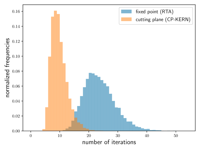
(a)

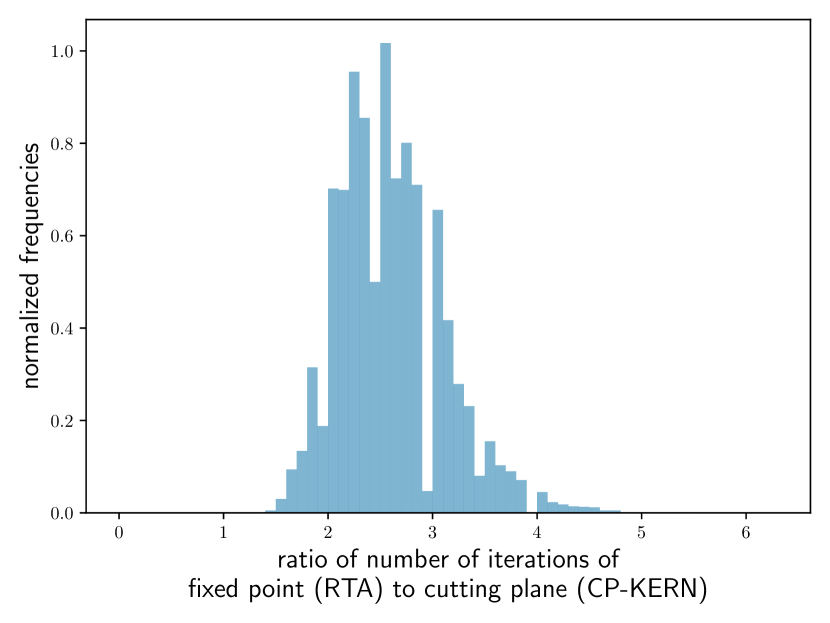
(b)

Figure 2. $n=25$, $\sum_{j\in[n-1]}U_{j}\approx 0.9$

We show various statistics for the number of iterations for $n=25$ and variable utilization in Table 4. We do the same for variable $n$ and $\sum_{j\in[n-1]}U_{j}\approx 0.8$ in Table 5. In all cases, CP-KERN has better statistics than RTA, e.g., smaller means and variances.

	(Min, Max)		Mean		Variance
$\sum_{j\in[n-1]}U_{j}$	RTA	CP-KERN	RTA	CP-KERN	RTA	CP-KERN
$0.9$	$(10,54)$	$(4,27)$	$23.29$	$9.29$	$29.49$	$7.71$
$0.8$	$(7,40)$	$(3,23)$	$14.93$	$6.91$	$10.20$	$3.60$
$0.7$	$(6,22)$	$(3,15)$	$11.28$	$5.68$	$4.84$	$2.14$

Table 4. Number of iterations for $n=25$ and variable utilization.

	(Min, Max)		Mean		Variance
$n$	RTA	CP-KERN	RTA	CP-KERN	RTA	CP-KERN
$25$	$(7,40)$	$(3,23)$	$14.93$	$6.91$	$10.20$	$3.60$
$50$	$(9,37)$	$(4,23)$	$17.21$	$8.82$	$10.72$	$5.30$
$75$	$(11,42)$	$(5,29)$	$18.60$	$10.02$	$11.86$	$6.85$

Table 5. Number of iterations for variable $n$ and $\sum_{j\in[n-1]}U_{j}\approx 0.8$.

6.4. Experiment II

In this experiment, we compare the running time of RTA to the running time of CP-KERN for synthetic instances of Problem (3). The initial value is the same as the one used in the previous experiment.

For $n=25$ and $\sum_{j\in[n-1]}U_{j}\approx 0.9$, we show histograms of the running times of CP-KERN and RTA in Figure 3(a). The histogram for CP-KERN is to the left of the histogram for RTA; thus, CP-KERN is faster than RTA. Both histograms have long tails, and most instances of the problem are solved within $20\mu s$ by both algorithms. We also show a histogram of the ratio of the CPU time of RTA to the CPU time of CP-KERN in Figure 3(b). Unlike, the previous experiment, the ratio is occasionally below one; thus, RTA is faster than CP-KERN for a small fraction of the generated instances. This is not an anomaly. In Section 5, we showed that CP-KERN and RTA have the same asymptotic worst-case running time, and CP-KERN, unlike RTA, has an optimal convergence rate; thus, theoretically, CP-KERN is superior to RTA. However, the theoretical analysis of the running time focuses on asymptotic worst-case running times and ignores implementation-dependent constants; thus, if the convergence rate of the two algorithms is similar on an instance, there RTA can be faster than CP-KERN. On average, CP-KERN is about $1.4$ times faster than RTA, and the maximum ratio is about $7$.

(a)

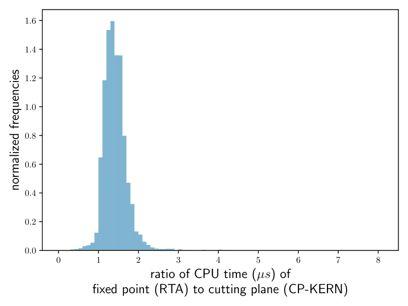
(b)

Figure 3. $n=25$, $\sum_{j\in[n-1]}U_{j}\approx 0.9$

We show various statistics for the running times of RTA and CP-KERN for $n=25$ and variable utilization in Table 6. We do the same for variable $n$ and $\sum_{j\in[n-1]}U_{j}\approx 0.8$ in Table 7. In all cases, CP-KERN has better statistics than RTA, e.g, smaller means and variances.

	(Min, Max)		Mean		Variance
$\sum_{j\in[n-1]}U_{j}$	RTA	CP-KERN	RTA	CP-KERN	RTA	CP-KERN
$0.9$	$(4.33,81.0)$	$(3.33,68.0)$	$9.62$	$6.94$	$11.65$	$6.74$
$0.8$	$(3.0,52.67)$	$(2.67,51.67)$	$6.26$	$5.19$	$4.84$	$3.44$
$0.7$	$(2.67,41.67)$	$(2.33,41.33)$	$4.85$	$4.38$	$2.86$	$2.13$

Table 6. CPU time ($\mu s$) for $n=25$ and variable utilization.

	(Min, Max)		Mean		Variance
$n$	RTA	CP-KERN	RTA	CP-KERN	RTA	CP-KERN
$25$	$(3.0,52.67)$	$(2.67,51.67)$	$6.26$	$5.19$	$4.84$	$3.44$
$50$	$(7.67,103.67)$	$(6.67,109.67)$	$13.75$	$12.04$	$16.29$	$11.58$
$75$	$(12.33,204.33)$	$(11.67,163.0)$	$21.83$	$20.31$	$32.93$	$27.55$

Table 7. CPU time ($\mu s$) for variable $n$ and $\sum_{j\in[n-1]}U_{j}\approx 0.8$.

6.5. Experiment III

In this experiment, we compare the number of iterations used by QPA to the number of iterations used by CP-KERN for synthetic instances of Problem (6). Since the total utilization is less than one in all our configurations, we use the initial value $L=L_{b}$ for both algorithms. In Appendix B, we show that the bound $L_{b}$ is implicitly used by CP-KERN and can also be explicitly passed to CP-KERN by using an alternative reduction from Problem (14) to the kernel.

For $n=25$, $\sum_{j\in[n]}U_{j}\approx 0.9$ and $\sum_{j\in[n]}\delta_{j}\approx 1.5$, we show histograms of the number of iterations of CP-KERN and QPA in Figure 4(a). The histogram for CP-KERN is to the left of the histogram for QPA; thus, CP-KERN has a better convergence rate than QPA. The histogram for CP-KERN is thinner and taller than the histogram for QPA. Therefore, the convergence rate of CP-KERN is more predictable than the convergence rate of QPA. We also show a histogram of the ratio of the number of iterations of QPA to the number of iterations of CP-KERN in Figure 4(b). As expected, the ratio is never below one. The average ratio is about $2.9$.

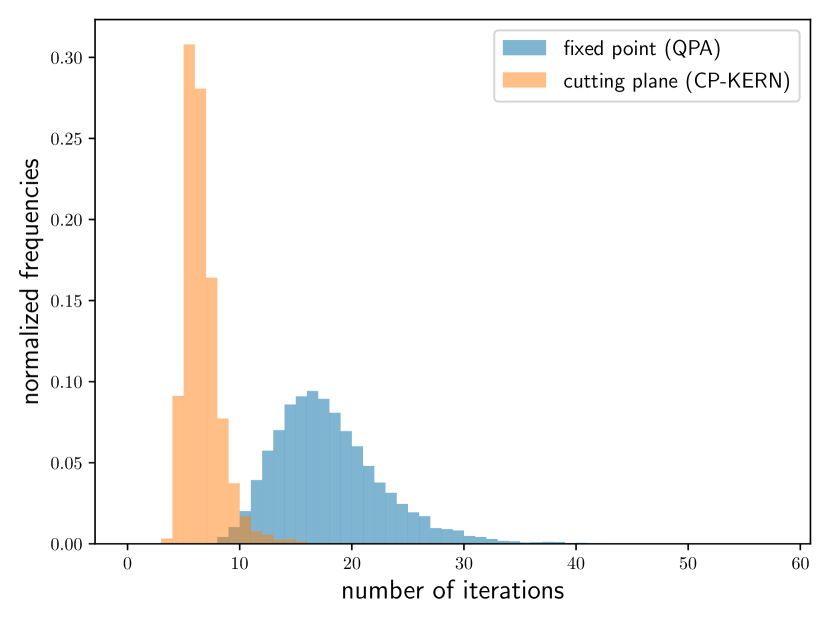
(a)

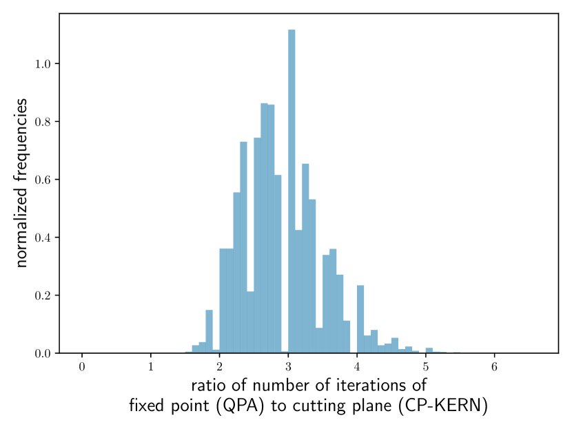
(b)

Figure 4. $n=25$, $\sum_{j\in[n]}U_{j}\approx 0.9$, $\sum_{j\in[n]}\delta_{j}\approx 1.5$

We show various statistics for variable utilization for a fixed configuration in Table 8. We do the same for variable density and variable $n$ in Tables 9 and 10 respectively. In all cases, CP-KERN has better statistics than QPA, e.g., smaller means and variances.

	(Min, Max)		Mean		Variance
$\sum_{j\in[n]}U_{j}$	QPA	CP-KERN	QPA	CP-KERN	QPA	CP-KERN
$0.9$	$(7,58)$	$(3,20)$	$17.51$	$6.14$	$24.44$	$2.73$
$0.8$	$(5,23)$	$(3,11)$	$10.35$	$4.51$	$4.76$	$0.56$
$0.7$	$(4,14)$	$(2,6)$	$7.80$	$4.02$	$1.87$	$0.29$

Table 8. Number of iterations for $n=25$, $\sum_{j\in[n]}\delta_{j}\approx 1.5$, and variable utilization.

	(Min, Max)		Mean		Variance
$\sum_{j\in[n]}\delta_{j}$	QPA	CP-KERN	QPA	CP-KERN	QPA	CP-KERN
$1.25$	$(5,30)$	$(2,11)$	$12.74$	$3.88$	$10.49$	$0.47$
$1.50$	$(7,58)$	$(3,20)$	$17.51$	$6.14$	$24.44$	$2.73$
$1.75$	$(9,67)$	$(4,28)$	$21.61$	$8.54$	$38.16$	$6.33$

Table 9. Number of iterations for $n=25$, $\sum_{j\in[n]}U_{j}\approx 0.9$, and variable density.

	(Min, Max)		Mean		Variance
$n$	QPA	CP-KERN	QPA	CP-KERN	QPA	CP-KERN
$25$	$(7,58)$	$(3,20)$	$17.51$	$6.14$	$24.44$	$2.73$
$50$	$(8,53)$	$(4,17)$	$17.40$	$6.06$	$11.52$	$1.10$
$75$	$(10,33)$	$(4,14)$	$17.35$	$6.05$	$7.21$	$0.65$

Table 10. Number of iterations for $\sum_{j\in[n]}U_{j}\approx 0.9$, $\sum_{j\in[n]}\delta_{j}\approx 1.5$, and variable $n$.

6.6. Experiment IV

In this experiment, we compare the running time of QPA to the running time of CP-KERN for synthetic instances of Problem (6). We use the same initial value as the previous section.

For $n=25$, $\sum_{j\in[n]}U_{j}\approx 0.9$ and $\sum_{j\in[n]}\delta_{j}\approx 1.5$, we show histograms of the running times of CP-KERN and QPA in Figure 5(a). The histogram for CP-KERN is to the left of the histogram for QPA; thus, CP-KERN is faster than QPA. Similar to Experiment II, most instances of the problem are solved within $20\mu s$ by both algorithms. We also show a histogram of the ratio of the running time of QPA to the running time of CP-KERN in Figure 5(b). QPA is faster than CP-KERN for a small fraction of the generated instances, but the average ratio is about $1.3$, and the maximum ratio is about $8$.

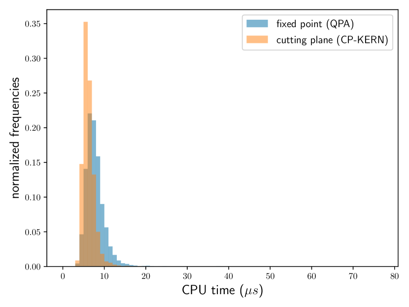
(a)

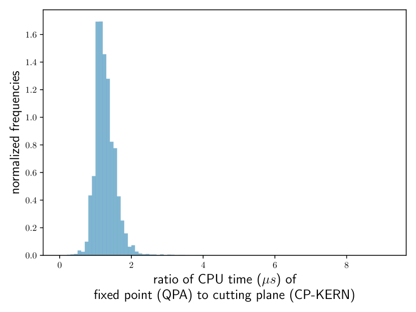
(b)

Figure 5. $n=25$, $\sum_{j\in[n]}U_{j}\approx 0.9$, $\sum_{j\in[n]}\delta_{j}\approx 1.5$

We show various statistics for variable utilization for a fixed configuration in Table 11. We do the same for variable density and variable $n$ in Tables 12 and 13 respectively. From the last rows of Tables 11 and 13, we can see that QPA is faster than CP-KERN for some configurations where the system utilization is small or $n$ is large. When the system utilization is small, then the denominator of $L_{b}$ is large, and hence $L_{b}$ is small; thus, the instances can be expected to be less challenging for both the algorithms (recall that $L$ occurs in the numerator in the asymptotic characterization of worst-case running times in Theorems 2.2 and 5.12). In Experiment II, we were able to control the hardness of the instances to some extent by choosing $D_{n}$ to be a large constant. Since we do not exercise any such control here, less challenging instances are produced in some cases. This explains why the simpler QPA outperforms the theoretically superior CP-KERN in the last configuration in Table 11. A similar explanation works for the last configuration in Table 13 as well. When $n=75$ and the total density is $1.75$, the deadlines are quite close to the periods, and hence the numerator of $L_{b}$ is small; thus, less challenging instances are generated. We have verified that CP-KERN is faster than QPA for $n=75$ and larger densities such as $5$.

	(Min, Max)		Mean		Variance
$\sum_{j\in[n]}U_{j}$	QPA	CP-KERN	QPA	CP-KERN	QPA	CP-KERN
$0.9$	$(3.0,76.67)$	$(3.0,50.0)$	$7.67$	$6.12$	$8.51$	$4.35$
$0.8$	$(2.33,39.33)$	$(2.67,40.33)$	$4.65$	$4.58$	$2.26$	$2.03$
$0.7$	$(1.67,29.67)$	$(2.33,39.0)$	$3.64$	$4.04$	$1.25$	$1.56$

Table 11. Running time for $n=25$, $\sum_{j\in[n]}\delta_{j}\approx 1.5$, and variable utilization.

	(Min, Max)		Mean		Variance
$\sum_{j\in[n]}\delta_{j}$	QPA	CP-KERN	QPA	CP-KERN	QPA	CP-KERN
$1.25$	$(2.33,56.67)$	$(2.33,42.0)$	$5.64$	$4.39$	$3.95$	$2.01$
$1.50$	$(3.0,76.67)$	$(3.0,50.0)$	$7.67$	$6.12$	$8.51$	$4.35$
$1.75$	$(4.0,121.67)$	$(3.0,87.67)$	$9.18$	$7.42$	$13.77$	$8.03$

Table 12. Running time for $n=25$, $\sum_{j\in[n]}U_{j}\approx 0.9$, and variable density.

	(Min, Max)		Mean		Variance
$n$	QPA	CP-KERN	QPA	CP-KERN	QPA	CP-KERN
$25$	$(3.0,76.67)$	$(3.0,50.0)$	$7.67$	$6.12$	$8.51$	$4.35$
$50$	$(6.33,132.33)$	$(8.0,122.67)$	$14.26$	$13.91$	$16.67$	$12.97$
$75$	$(11.67,163.67)$	$(14.67,178.0)$	$20.66$	$22.22$	$19.41$	$18.29$

Table 13. Running time for $\sum_{j\in[n]}U_{j}\approx 0.9$, $\sum_{j\in[n]}\delta_{j}\approx 1.5$, and variable $n$.

7. Conclusion

We have achieved a logical unification of four different algorithms (RTA, IP-FP, QPA, IP-EDF) by showing that they all belong to a family of cutting-plane algorithms. CP-KERN has the optimal convergence rate in the family; RTA and QPA have suboptimal convergence rates. In theory, CP-KERN, RTA and QPA have the same worst-case running times. The empirical evaluations show that

• CP-KERN has higher convergence rates than RTA and QPA for randomly generated systems.

• CP-KERN has smaller running times than RTA and QPA for randomly generated systems that are hard.

Unlike the convergence rates, the running times can vary a lot depending on low-level implementation choices.

For any given schedulability problem instance, the number of iterations required for convergence is a good machine-independent measure of the hardness of the instance, especially for methods that proceed by estimating dual bounds. Using the number of iterations as a measure of the hardness of a schedulability instance is similar to counting the number of recursive calls to the Davis-Putnam (DP) procedure for SAT instances (Selman et al., 1996), especially when one considers the connections between DP, resolution, and cutting planes (Chvátal, 1973; Cook et al., 1987; Hooker, 1988). We plan to investigate these connections in future work to understand how to generate hard schedulability instances.

Our cutting planes for schedulability problems are quite similar to textbook cutting planes like Gomory cuts. A different approach towards generating cuts is the so-called polyhedral approach wherein facet-defining inequalities are used instead of traditional textbook cutting planes (Padberg and Rinaldi, 1991). The polyhedral approach has been used successfully to understand scheduling models in the OR community (Queyranne and Schulz, 1996; van den Akker et al., 1999). In future work, we hope to apply the polyhedral approach to schedulability problems.

Most efforts to improve the running times of the fixed-point iteration tests have focused on finding a good initial guess for the fixed point (Sjodin and Hansson, 1998; Bril et al., 2003; Davis et al., 2008). Since we have shown that fixed-point iteration tests are special cases of cutting-plane algorithms, ideas like preprocessing and branch-and-cut can be experimented with to speed up schedulability tests. We expect branch-and-cut adaptations of CP-KERN to be much faster than CP-KERN, RTA, and QPA, especially if the tests can utilize multiple processors and if we are satisfied with feasible solutions to Problems (3) and (6).

Acknowledgments

The author would like to thank anonymous reviewers for their valuable suggestions. The author would also like to thank Pontus Ekberg and Sanjoy Baruah for discussions on the subject.

Declarations

This work is supported by the US National Science Foundation under Grant numbers CPS-1932530 and CNS-2141256.

Appendix A Properties of $f$

We establish basic properties of $f$ (Definition (23)) in the context of the kernel. We also assume that the vectors $T$, $U$, $\alpha$, and $\underline{x}$ are sorted in a nonincreasing order using the key $T_{j}\underline{x}_{j}-\alpha_{j}$ for each $j\in[n]$.

Lemma A.1.

For any $k\in[n]$, if $f(k-1)$ is well-defined, then we must have

$$\frac{f(k)-f(k-1)}{U_{k}}=\frac{\underline{x}_{k}T_{k}-\alpha_{k}-f(k)}{1-\sum_{j\in[n]\setminus[k-1]}U_{j}}=\frac{\underline{x}_{k}T_{k}-\alpha_{k}-f(k-1)}{1-\sum_{j\in[n]\setminus[k]}U_{j}}.$$

From the identities, it follows that

$$\operatorname{sgn}(f(k)-f(k-1))=\operatorname{sgn}(\underline{x}_{k}T_{k}-\alpha_{k}-f(k))=\operatorname{sgn}(\underline{x}_{k}T_{k}-\alpha_{k}-f(k-1)).$$

Proof Sketch.

Consider the following equations:

$$(1-\textstyle\sum_{j\in[n]\setminus[k-1]}U_{j})(f(k)-f(k-1))$$

$$= (1-\textstyle\sum_{j\in[n]\setminus[k]}U_{j})f(k)-(1-\textstyle\sum_{j\in[n]\setminus[k-1]}U_{j})f(k-1)-U_{k}f(k)$$

$$= (\beta+\textstyle\sum_{j\in[n]\setminus[k]}\alpha_{j}U_{j}+\textstyle\sum_{j\in[k]}\underline{x}_{j}C_{j})-$$

$$(\beta+\textstyle\sum_{j\in[n]\setminus[k-1]}\alpha_{j}U_{j}+\textstyle\sum_{j\in[k-1]}\underline{x}_{j}C_{j})-U_{k}f(k)$$ (using Definition (23))

$$= \underline{x}_{k}C_{k}-\alpha_{k}U_{k}-U_{k}f(k)$$

$$= U_{k}(\underline{x}_{k}T_{k}-\alpha_{k}-f(k))$$

From the definition of the kernel and the well-definedness of $f(k-1)$, we have $U_{k}>0$ and $1-\sum_{j\in[n]\setminus[k-1]}U_{j}>0$. Combining these facts with the above equations gives

$$\operatorname{sgn}(f(k)-f(k-1))=\operatorname{sgn}(\underline{x}_{k}T_{k}-\alpha_{k}-f(k)).$$

Similarly, we can show that

$$(1-\textstyle\sum_{j\in[n]\setminus[k]}U_{j})(f(k)-f(k-1))=U_{k}(\underline{x}_{k}T_{k}-\alpha_{k}-f(k-1)),$$

and the statement about the signs of various expressions follows from the positivity of the excluded expressions. ∎

Lemma A.2.

If $f$ has a local minimum point at $i$ in the interior of its domain, then we must have

$$f(i-1)=f(i)=f(i+1).$$

Proof sketch.

Assume that $i$ is a local minimum point of $f$ in the interior of its domain. From Lemma A.1, we get

$$\underline{x}_{i}T_{i}-\alpha_{i}\leq f(i)\leq\underline{x}_{i+1}T_{i+1}-\alpha_{i+1}.$$

From the order imposed on the vectors by sorting, it follows that $\underline{x}_{i+1}T_{i+1}-\alpha_{i+1}\leq\underline{x}_{i}T_{i}-\alpha_{i}$. Combining the three inequalities gives

$$\underline{x}_{i}T_{i}-\alpha_{i}=f(i)=\underline{x}_{i+1}T_{i+1}-\alpha_{i+1}.$$

Using Lemma A.1 again, we must have

$$f(i-1)=f(i)=f(i+1).$$

∎

The absence of strict local minimum points in the interior of $f$ trivially implies the following corollary.

Corollary A.3.

If $f$ has two local maximum points $i_{1}$ and $i_{2}$ in $\{0\}\cup[n]$ with $i_{1}\leq i_{2}$, then we must have

$$\forall i\in[i_{2}]\setminus[i_{1}]:f(i)=f(i_{1}).$$

In other words, any local maximum point of $f$ is a global maximum point of $f$, and $f$ is constant between two local maximum points.

Appendix B On initial values of fixed-point iteration approaches

Problem (3) can be reduced to the kernel by initializing $(n,\alpha,\beta,a,b)$ in the target instance to $(n,J,0,1,D_{n}-J_{n})$. Recall that $\operatorname{rbf}$ is given by

$$t\mapsto\sum_{j\in[n]}\left\lceil\frac{t+J_{j}}{T_{j}}\right\rceil C_{j}.$$

Since we are only concerned about the behavior of $\operatorname{rbf}$ for the domain $\interval{1}{D_{n}-J_{n}}$, we must have

$$t+J_{n}\leq D_{n}\leq T_{n}$$

The second inequality is true because we have assumed that the FP system has constrained deadlines. Thus, $\lceil(t+J_{n})/T_{n}\rceil=1$ and $\operatorname{rbf}$ can be simplified to

$$t\mapsto C_{n}+\sum_{j\in[n-1]}\left\lceil\frac{t+J_{j}}{T_{j}}\right\rceil C_{j}.$$

The schedulability condition can be written as

$$\exists t\in\interval{C_{n}}{D_{n}-J_{n}}:C_{n}+\sum_{j\in[n-1]}\left\lceil\frac{t+J_{j}}{T_{j}}\right\rceil C_{j}\leq t.$$ (26)

Using this schedulability condition, we can reduce Problem (3) to the kernel by initializing $(n,\alpha,\beta,a,b)$ in the target instance to $(n-1,J,C_{n},C_{n},D_{n}-J_{n})$.

When we solve the target instance using CP-KERN, $f$ is given by

$$k\mapsto\frac{C_{n}+\sum_{j\in[n-1]\setminus[k]}J_{j}U_{j}+\sum_{j\in[k]}\underline{x}_{j}C_{j}}{1-\sum_{j\in[n-1]\setminus[k]}U_{j}}$$ (27)

In each iteration of CP-KERN, the value $t^{*}=\max f$ is at least

$$f(0)=\frac{C_{n}+\sum_{j\in[n-1]}J_{j}U_{j}}{1-\sum_{j\in[n-1]}U_{j}}$$ (28)

$f(0)$ has been proposed as an initial value for RTA in prior work by using a different analysis method (Sjodin and Hansson, 1998). However, we do not need to pass this initial bound to CP-KERN since it finds it implicitly; on the other hand, initializing $(n,\alpha,\beta,a,b)$ in the target instance to $(n-1,J,C_{n},\lceil f(0)\rceil,D_{n}-J_{n})$ is a valid reduction from Problem (3) to the kernel.

Problem (14) (the $k$-th subproblem of EDF schedulability) can be solved by reducing it to the kernel by setting $(n,\alpha,\beta,a,b)$ to $(k,D-T-J,1,-b_{k}+1,-a_{k})$. When we solve the target instance by using CP-KERN, $f$ is given by

$$\ell\mapsto\frac{1+\sum_{j\in[k]\setminus[\ell]}(\hat{D}_{j}-T_{j})U_{j}+\sum_{j\in[\ell]}\underline{x}_{j}C_{j}}{1-\sum_{j\in[k]\setminus[\ell]}U_{j}}$$ (29)

In each iteration of CP-KERN, the value $t^{*}=\max f$ is at least

$$f(0)=\frac{\sum_{j\in[k]}(\hat{D}_{j}-T_{j})U_{j}-1}{1-\sum_{j\in[k]}U_{j}}$$ (30)

Since the sign of $t$ was inverted in the reduction to the kernel, $-f(0)$ is an upper bound for $t$ in Problem (14). It is not too hard to see that the upper bound $L_{b}$ (see Definition (8)) is implicitly present in $-f(0)$ when $k=n$. Since $f(0)$ is a lower bound for $t$ in the kernel, when reducing Problem (14) to the kernel, $(n,\alpha,\beta,a,b)$ in the target instance can be initialized to $(k,\hat{D}-T,1,\max(-b_{k}+1,\lceil f(0)\rceil),-a_{k})$.

Appendix C IP formulations for asynchronous EDF schedulability

If the first request for a periodic task $i$ arrives at time $O_{i}$, then $O_{i}$ is called the phase or arrival offset of task $i$. If all tasks in a system have equal phases (in which case they are typically assumed to be equal to zero and omitted from the specifications), then it is called a synchronous system; otherwise, it is called an asynchronous system. In this section, we assume that the tasks are periodic and asynchronous with zero release jitter. Such a system is unschedulable if and only if $\sum_{i\in[n]}U_{i}>1$ or

$$\exists t_{1},t_{2}\in\interval{0}{O_{\max}+2\mathcal{T}}\cap\mathbb{Z}:\ \sum_{i\in[n]}\eta_{i}(t_{1},t_{2})C_{i}>t_{2}-t_{1}\geq 0$$ (31)

holds (Baruah et al., 1990a, Lem. 3.4), where

$$\eta_{i}(t_{1},t_{2})=\lvert\{k\in\mathbb{N}\mid t_{1}\leq O_{i}+kT_{i},O_{i}+kT_{i}+D_{i}\leq t_{2}\}\rvert$$ (32)

Thus, $\eta_{i}(t_{1},t_{2})$ is the number of times task $i$ has both its release time and deadline in $\interval{t_{1}}{t_{2}}$.

For such asynchronous systems, Baruah et al. (1990a) formulate (informally) Condition (31) as an integer program in Thm. 3.5. However, the formulation is flawed: this can be verified by applying the formulation on the system in Table 3.

$\eta_{i}$ can be simplified by considering three cases. If $t_{1}\leq O_{i}$ and $O_{i}+D_{i}\leq t_{2}$, then we have

$$\eta_{i}(t_{1},t_{2})=\left\lfloor\frac{t_{2}+T_{i}-D_{i}-O_{i}}{T_{i}}\right\rfloor.$$

Otherwise, if $t_{2}>O_{i}$ and $t_{2}-t_{1}\geq D_{i}$, then we have

$$\eta_{i}(t_{1},t_{2})=\left\lfloor\frac{t_{2}+T_{i}-D_{i}-O_{i}}{T_{i}}\right\rfloor-\left\lceil\frac{t_{1}-O_{i}}{T_{i}}\right\rceil.$$

Otherwise, we have

$$\eta_{i}(t_{1},t_{2})=0.$$

A branching strategy, like the one we used in Section 4.2, follows straightforwardly from the three conditions, resulting in $\mathcal{O}(n^{3})$ subproblems with simple IP formulations.

References

- Audsley et al. (1993) N. Audsley, A. Burns, M. Richardson, K. Tindell, and A. J. Wellings. Applying new scheduling theory to static priority pre-emptive scheduling. Software Engineering Journal, 8(5):284–292, September 1993. ISSN 2053-910X. doi:10.1049/sej.1993.0034.
- Audsley et al. (1995) Neil C. Audsley, Alan Burns, Robert I. Davis, Ken W. Tindell, and Andy J. Wellings. Fixed priority pre-emptive scheduling: An historical perspective. Real-Time Systems, 8(2-3):173–198, 1995. ISSN 0922-6443, 1573-1383. doi:10.1007/BF01094342.
- Baruah and Fisher (2005) Sanjoy Baruah and N. Fisher. Real-time scheduling of sporadic task systems when the number of distinct task types is small. In 11th IEEE International Conference on Embedded and Real-Time Computing Systems and Applications (RTCSA’05), pages 232–237, August 2005. doi:10.1109/RTCSA.2005.75.
- Baruah et al. (2022) Sanjoy Baruah, Pontus Ekberg, and Abhishek Singh. Fixed-Parameter Analysis of Preemptive Uniprocessor Scheduling Problems. In 2022 IEEE Real-Time Systems Symposium, page 12, 2022.
- Baruah et al. (1990a) Sanjoy K. Baruah, Louis E. Rosier, and Rodney R. Howell. Algorithms and complexity concerning the preemptive scheduling of periodic, real-time tasks on one processor. Real-Time Systems, 2(4):301–324, November 1990a. ISSN 1573-1383. doi:10.1007/BF01995675.
- Baruah et al. (1990b) S.K. Baruah, A.K. Mok, and L.E. Rosier. Preemptively scheduling hard-real-time sporadic tasks on one processor. In [1990] Proceedings 11th Real-Time Systems Symposium, pages 182–190, December 1990b. doi:10.1109/REAL.1990.128746.
- Bini and Buttazzo (2004) E. Bini and G.C. Buttazzo. Schedulability analysis of periodic fixed priority systems. IEEE Transactions on Computers, 53(11):1462–1473, November 2004. ISSN 1557-9956. doi:10.1109/TC.2004.103.
- Bini (2019) Enrico Bini. Cutting the Unnecessary Deadlines in EDF. In 2019 IEEE 25th International Conference on Embedded and Real-Time Computing Systems and Applications (RTCSA), pages 1–8, August 2019. doi:10.1109/RTCSA.2019.8864569.
- Boussinot and de Simone (1991) F. Boussinot and R. de Simone. The ESTEREL language. Proceedings of the IEEE, 79(9):1293–1304, September 1991. ISSN 1558-2256. doi:10.1109/5.97299.
- Bril et al. (2003) R.J. Bril, W.F.J. Verhaegh, and E.-J.D. Pol. Initial values for online response time calculations. In 15th Euromicro Conference on Real-Time Systems, 2003. Proceedings., pages 13–22, July 2003. doi:10.1109/EMRTS.2003.1212722.
- Bubeck (2015) Sébastien Bubeck. Convex Optimization: Algorithms and Complexity, November 2015. URL http://arxiv.org/abs/1405.4980. arXiv:1405.4980 [cs, math, stat].
- Burden and Faires (2011) Richard L. Burden and J. Douglas Faires. Numerical analysis. Cengage Learning, USA, 9 edition, 2011. ISBN 978-0-538-73351-9.
- Buttazzo (2005) Giorgio C. Buttazzo. Rate Monotonic vs. EDF: Judgment Day. Real-Time Systems, 29(1):5–26, January 2005. ISSN 1573-1383. doi:10.1023/B:TIME.0000048932.30002.d9.
- Buttazzo (2011) Giorgio C. Buttazzo. Hard Real-Time Computing Systems: Predictable Scheduling Algorithms and Applications. Springer Publishing Company, Incorporated, 3rd edition, 2011. ISBN 978-1-4614-0675-4.
- Chvátal (1973) V. Chvátal. Edmonds polytopes and a hierarchy of combinatorial problems. Discrete Mathematics, 4(4):305–337, April 1973. ISSN 0012-365X. doi:10.1016/0012-365X(73)90167-2. URL https://www.sciencedirect.com/science/article/pii/0012365X73901672.
- Cook et al. (1987) W. Cook, C. R. Coullard, and Gy. Turán. On the complexity of cutting-plane proofs. Discrete Applied Mathematics, 18(1):25–38, September 1987. ISSN 0166-218X. doi:10.1016/0166-218X(87)90039-4. URL https://www.sciencedirect.com/science/article/pii/0166218X87900394.
- Cook et al. (2013) William Cook, Thorsten Koch, Daniel E. Steffy, and Kati Wolter. A hybrid branch-and-bound approach for exact rational mixed-integer programming. Mathematical Programming Computation, 5(3):305–344, September 2013. ISSN 1867-2957. doi:10.1007/s12532-013-0055-6. URL https://doi.org/10.1007/s12532-013-0055-6.
- Dantzig (1987) George B. Dantzig. Origins of the Simplex Method. Technical Report SOL 87-5, Department of Operations Research, Stanford University, May 1987. URL https://apps.dtic.mil/sti/citations/ADA182708. Section: Technical Reports.
- Davis et al. (2008) Robert I. Davis, Attila Zabos, and Alan Burns. Efficient Exact Schedulability Tests for Fixed Priority Real-Time Systems. IEEE Transactions on Computers, 57(9):1261–1276, September 2008. ISSN 1557-9956. doi:10.1109/TC.2008.66.
- Eifler and Gleixner (2023) Leon Eifler and Ambros Gleixner. A computational status update for exact rational mixed integer programming. Mathematical Programming, 197(2):793–812, February 2023. ISSN 1436-4646. doi:10.1007/s10107-021-01749-5. URL https://doi.org/10.1007/s10107-021-01749-5.
- Ekberg and Yi (2017) Pontus Ekberg and Wang Yi. Fixed-Priority Schedulability of Sporadic Tasks on Uniprocessors is NP-Hard. In 2017 IEEE Real-Time Systems Symposium (RTSS), pages 139–146, December 2017. doi:10.1109/RTSS.2017.00020.
- George et al. (1996) Laurent George, Nicolas Rivierre, and Marco Spuri. Preemptive and Non-Preemptive Real-Time UniProcessor Scheduling. Report, INRIA, 1996.
- Griffin et al. (2020) David Griffin, Iain Bate, and Robert I. Davis. Generating Utilization Vectors for the Systematic Evaluation of Schedulability Tests. In 2020 IEEE Real-Time Systems Symposium (RTSS), pages 76–88, December 2020. doi:10.1109/RTSS49844.2020.00018.
- Grötschel et al. (1993) Martin Grötschel, László Lovász, and Alexander Schrijver. Geometric Algorithms and Combinatorial Optimization, volume 2 of Algorithms and Combinatorics. Springer, Berlin, Heidelberg, 1993. ISBN 978-3-642-78242-8 978-3-642-78240-4. doi:10.1007/978-3-642-78240-4.
- Hooker (1988) J. N. Hooker. Generalized resolution and cutting planes. Annals of Operations Research, 12(1):217–239, December 1988. ISSN 1572-9338. doi:10.1007/BF02186368. URL https://doi.org/10.1007/BF02186368.
- Joseph and Pandya (1986) M. Joseph and P. Pandya. Finding Response Times in a Real-Time System. The Computer Journal, 29(5):390–395, January 1986. ISSN 0010-4620. doi:10.1093/comjnl/29.5.390.
- Karmarkar (1984) N. Karmarkar. A new polynomial-time algorithm for linear programming. Combinatorica, 4(4):373–395, December 1984. ISSN 1439-6912. doi:10.1007/BF02579150. URL https://doi.org/10.1007/BF02579150.
- Khachiyan (1980) L. G. Khachiyan. Polynomial algorithms in linear programming. USSR Computational Mathematics and Mathematical Physics, 20(1):53–72, January 1980. ISSN 0041-5553. doi:10.1016/0041-5553(80)90061-0.
- Lehoczky et al. (1989) J. Lehoczky, L. Sha, and Y. Ding. The rate monotonic scheduling algorithm: Exact characterization and average case behavior. In [1989] Proceedings. Real-Time Systems Symposium, pages 166–171, December 1989. doi:10.1109/REAL.1989.63567.
- Lenstra (1983) H. W. Lenstra. Integer Programming with a Fixed Number of Variables. Mathematics of Operations Research, 8(4):538–548, 1983. ISSN 0364-765X.
- Levy and Tian (2020) David Charles Levy and Yu-Chu Tian. Handbook of Real-Time Computing. Springer Singapore, 2020.
- Liu and Layland (1973) C. L. Liu and James W. Layland. Scheduling Algorithms for Multiprogramming in a Hard-Real-Time Environment. Journal of the ACM, 20(1):46–61, January 1973. ISSN 0004-5411. doi:10.1145/321738.321743.
- Liu (2000) Jane W. S. W. Liu. Real-Time Systems. Prentice Hall PTR, USA, 1st edition, 2000. ISBN 978-0-13-099651-0.
- Lu et al. (2006) Wan-Chen Lu, Jen-Wei Hsieh, and Wei-Kuan Shih. A precise schedulability test algorithm for scheduling periodic tasks in real-time systems. In Proceedings of the 2006 ACM Symposium on Applied Computing, SAC ’06, pages 1451–1455, New York, NY, USA, April 2006. Association for Computing Machinery. ISBN 978-1-59593-108-5. doi:10.1145/1141277.1141616.
- Manabe and Aoyagi (1998) Yoshifumi Manabe and Shigemi Aoyagi. A Feasibility Decision Algorithm for Rate Monotonic and Deadline Monotonic Scheduling. Real-Time Systems, 14(2):171–181, March 1998. ISSN 1573-1383. doi:10.1023/A:1007964900035.
- Matoušek and Gärtner (2007) Jiří Matoušek and Bernd Gärtner. Understanding and Using Linear Programming. Universitext. Springer Berlin, Heidelberg, first edition, 2007. ISBN 978-3-540-30717-4.
- Mattingley and Boyd (2012) Jacob Mattingley and Stephen Boyd. CVXGEN: A code generator for embedded convex optimization. Optimization and Engineering, 13(1):1–27, March 2012. ISSN 1573-2924. doi:10.1007/s11081-011-9176-9.
- Nguyen et al. (2022) Thi Huyen Chau Nguyen, Werner Grass, and Klaus Jansen. Exact Polynomial Time Algorithm for the Response Time Analysis of Harmonic Tasks. In Cristina Bazgan and Henning Fernau, editors, Combinatorial Algorithms, Lecture Notes in Computer Science, pages 451–465, Cham, 2022. Springer International Publishing. ISBN 978-3-031-06678-8. doi:10.1007/978-3-031-06678-8_33.
- Padberg and Rinaldi (1991) Manfred Padberg and Giovanni Rinaldi. A Branch-and-Cut Algorithm for the Resolution of Large-Scale Symmetric Traveling Salesman Problems. SIAM Review, 33(1):60–100, 1991. ISSN 0036-1445. URL http://www.jstor.org/stable/2030652. Publisher: Society for Industrial and Applied Mathematics.
- Park and Baek (2023) Moonju Park and Hyeongboo Baek. Determining rate monotonic schedulability of real-time periodic tasks using continued fractions. Information Processing Letters, 179:106296, January 2023. ISSN 0020-0190. doi:10.1016/j.ipl.2022.106296.
- Perale and Vardanega (2021) D. Perale and T. Vardanega. Removing bias from the judgment day: A Ravenscar-based toolbox for quantitative comparison of EDF-to-RM uniprocessor scheduling. Journal of Systems Architecture, 119:102236, October 2021. ISSN 1383-7621. doi:10.1016/j.sysarc.2021.102236.
- Queyranne and Schulz (1996) Maurice Queyranne and Andreas S Schulz. Polyhedral Approaches to Machine Scheduling, 1996.
- Ripoll et al. (1996) Ismael Ripoll, Alfons Crespo, and Aloysius K. Mok. Improvement in feasibility testing for real-time tasks. Real-Time Systems, 11(1):19–39, July 1996. ISSN 1573-1383. doi:10.1007/BF00365519.
- Rivas et al. (2011) Juan M. Rivas, J. Javier Gutierrez, J. Carlos Palencia, and Michael Gonz´lez Harbour. Schedulability Analysis and Optimization of Heterogeneous EDF and FP Distributed Real-Time Systems. In 2011 23rd Euromicro Conference on Real-Time Systems, pages 195–204, July 2011. doi:10.1109/ECRTS.2011.26.
- Selman et al. (1996) Bart Selman, David G. Mitchell, and Hector J. Levesque. Generating hard satisfiability problems. Artificial Intelligence, 81(1):17–29, March 1996. ISSN 0004-3702. doi:10.1016/0004-3702(95)00045-3. URL https://www.sciencedirect.com/science/article/pii/0004370295000453.
- Sha et al. (2004) Lui Sha, Tarek Abdelzaher, Karl-Erik årzén, Anton Cervin, Theodore Baker, Alan Burns, Giorgio Buttazzo, Marco Caccamo, John Lehoczky, and Aloysius K. Mok. Real Time Scheduling Theory: A Historical Perspective. Real-Time Systems, 28(2):101–155, November 2004. ISSN 1573-1383. doi:10.1023/B:TIME.0000045315.61234.1e.
- Singh (2023) Abhishek Singh. abhcs/rtsched: v0.1.2, May 2023. URL https://doi.org/10.5281/zenodo.7938966.