The experimental data from VENUS, TOPAS, OPAL, DELPHI, ALEPH and L3 collaborations, collected from 1989 to 2003, are applied to study the QED framework through direct contact interaction terms approach, using the annihilation reaction $\rm e^{+}e^{-}\rightarrow\gamma\gamma(\gamma)$. The analysis involves performing of a $\chi^{2}$ test to detect the presence of an excited electron $e^{*}$ and evidence of non-point like behavior in the $e^{+}e^{-}$ annihilation zone. The results of the analysis indicate a strong signal, with a confidence level of approximately $5\sigma$, for the presence of an excited electron with a mass of $308\pm 14$ GeV, and a deviation from a point-like behavior of the charge distribution of the electron. The radius of this deviation is $1.57\pm 0.07\times 10^{-17}$ cm, which can be interpreted as the size of the electron.

Keywords: QED; Contact interaction; Beyond standard model

March 2023

1 Introduction

The electron is one of the most fundamental building blocks of matter, and its discovery over a century ago revolutionized our understanding of the physical world. Since then, it has been the subject of countless investigations, revealing properties that continue to challenge our understanding of nature at the deepest level. A historical account of the electron’s discovery and subsequent study can provide valuable insights into the foundations of modern particle physics.

In 1785, the discovery of Coulomb’s law and in 1820, the discovery of magnetism paved the way for investigating charged particle beams with Cathode Ray Tubes. By 1869, this possibility was realized.

Charles-Augustin de Coulomb’s law states that the magnitude of the electrostatic force between two point charges is directly proportional to the product of the charges and inversely proportional to the square of the distance between them [1].

Three discoveries made in 1820 laid the groundwork for magnetism. Firstly, Hans Christian $\ddot{\rm O}$rsted demonstrated that a current-carrying wire produces a circular magnetic field around it [2]. Secondly, Andr’e-Marie Amp‘ere showed that parallel wires with currents attract each other if the currents flow in the same direction, and repel if they flow in opposite directions [3]. Thirdly, Jean-Baptiste Biot and F’elix Savart determined experimentally the forces that a current-carrying long, straight wire exerts on a small magnet. They found that the forces were inversely proportional to the perpendicular distance from the wire to the magnet [4].

Cathode rays, also known as electron beams or e-beams, are streams of electrons observed in discharge tubes. They are produced by applying a voltage across two electrodes in an evacuated glass tube, causing electrons to be emitted from the cathode (the negative electrode). The phenomenon was first observed in 1869 by Julius Pl”ucker and Johann Wilhelm Hittorf [5] and later named ”cathode rays” (Kathodenstrahlen) [6] by Eugen Goldstein in 1876. In 1897, J. J. Thomson discovered that cathode rays were composed of negatively charged particles, later named electrons. Cathode-ray tubes (CRTs) use a focused beam of electrons deflected by electric or magnetic fields to create images on a screen [7].

Sir Joseph John Thomson credited in 1897 with the discovery of the electron, the first subatomic particle being discovered. He showed that cathode rays were composed of previously unknown negatively charged particles, which must have bodies much smaller than atoms and a very large charge-to-mass ratio [8]. Finally, Millikan and Fletcher measured in 1909 the mass and charge separately in the oil drop experiment [9].

After the discovery of the electron, Abraham [10] and Lorentz [11, 12] proposed the first models of the electron as an extended spherical electrical charged object with its total energy concentrated in the electric field, in 1903. However, these models were based on the assumption of a homogeneous distribution of charge density. Although, the model provided a means of explaining the electromagnetic origin of the electron’s mass, it also raised the problem of preventing the electron from flying apart under the influence of Coulomb repulsion. Abraham proposed a solution to this inconsistency by suggesting that non-electromagnetic forces (like, for example, the Poincare stress) were necessary to prevent the electron from exploding. One may say that at that time, modeling the electron within the framework of electromagnetism was deemed impossible. Later, Dirac [13] proposed a point-like model of the electron and recognized the appealing aspect of the Lorentz model [11] regarding the electromagnetic origin of the electron’s mass. Nonetheless, at that time, this idea was found to be inconsistent with the existence of the neutron. Dirac highlighted in his paper [13] that although the electron can be treated as a point charge to avoid difficulties with the infinite Coulomb energy in equations, its finite size reappears in a new sense in the physical interpretation. Specifically, the interior of the electron can be viewed as a region of space through which signals can be transmitted faster than light.

Arthur Compton firstly introduced the idea of electron spin in 1921. In a paper on investigations of ferromagnetic substances with X-rays [14], he wrote: “Perhaps the most natural, and certainly the most generally accepted view of the nature of the elementary magnet, is that the revolution of electrons in orbits within the atom give to the atom as a whole the properties of a tiny permanent magnet ”. The electron’s magnetic moment $\mu_{s}$ is related to its spin $S$ through $\mu_{s}=-g_{s}\mu_{B}S/\hbar$, where $g_{s}\approx 2$. The Stern-Gerlach experiment, first proposed by Otto Stern in 1921 and conducted by Walther Gerlach in 1922 [15], inferred the existence of quantized electron spin angular momentum. In the experiment, spatially varying magnetic fields deflected silver atoms with non-zero magnetic moments on their way to a glass slide detector screen, providing evidence for the existence of electron spin. The existence of electron spin can also be inferred theoretically from the spin-statistics theorem and the Pauli exclusion principle. Conversely, given the electron’s spin, one can derive the Pauli exclusion principle [15, 16].

The existence of quantized particle spin allows for the possibility of investigating spin-dependent interactions by scattering polarized particle beams on different targets. In nuclear physics, scattering experiments use polarized beams [17] sources by electrostatic accelerators such as Tandem accelerators, which can achieve a range of center-of-mass energies from 1.2 MeV [18] to 20 MeV [19]. There are three types of polarized beams that have been developed: the atomic beam source, which uses the technique of the Stern-Gerlach experiment [20], the Lamb-shift source [22] developed after the discovery of the Lamb shift in 1947 [21], and the crossed-beam source [23].

Since 1926, various classical models of spinning point particles have been developed. However, these models face the challenge of constructing a stable point-like particle that includes a single repulsive Coulomb force over a range from zero to infinity.

One model of point-like particle related to electron spin is the Schr$\ddot{\rm o}$dinger suggestion [24] that connects electron spin with its Zitterbewegung motion - a trembling motion due to the rapid oscillation of a spinning particle about its classical worldline. The Zitterbewegung concept was motivated by attempts to understand the intrinsic nature of electron spin and involved fundamental studies in quantum mechanics [25].

Other types of classical models of point-like spinning particles has been developed. The Yang-Mills model, which is a class of gauge theories that describe the strong and electroweak interactions in the Standard Model of particle physics. The Weyl model is a spinor field theory that describes massless spin-1/2 particles that do not follow the Dirac equation. The Thirring model is a 1+1 dimensional field theory that describes a system of Dirac fermions coupled to a massless bosonic field. It is exactly solvable and has been used as a toy model for studying many-body problems in condensed matter physics. The Gross-Neveu model is a 2+1 dimensional field theory that describes a system of fermions with an interaction term that is quadratic in the fermion field. It is also exactly solvable and has been used to study critical phenomena in condensed matter physics. The Proca model is a relativistic quantum mechanical model that describes a massive vector boson. It is used to describe the massive vector bosons in the electroweak interaction and has been used extensively in the development of the Standard Model. There are many reviews and textbooks that cover the different classical models of point-like spinning particles. Some examples include [26, 27, 28, 29, 30]. In general, such kind of models encounter the problem of divergent self-energy for a point charge and approach this problem in the frame of various generalizations of the classical Lagrangian terms with higher derivatives or extra variables [31] and then restricting undesirable effects by applying geometrical [32] or symmetry [33] constraints.

The discovery of the Kerr-Newman solution to the Einstein-Maxwell equations in 1965 led to new possibilities for investigating the electron’s structure. Recently, this solution has been used in [35] to propose a model that considers the interplay between electrodynamics and gravity in the electron’s structure. Coupling electrodynamics with gravity introduces the geometry of De Sitter spaces [46], which provides attractive/repulsive forces dependent on distance from the origin and can distinguish between Schwarzschild and De Sitter black holes, ensuring the electron’s stability from the Coulomb repulsion. The theoretical aspects of whether the electron is point-like or not are discussed in [47].

The modeling of electron structure is driven by the desire to understand fundamental issues, such as the number of fermion families, fermion mass hierarchy, and mixing properties, that the Standard Model cannot explain. For example, a natural consequence of the so-called composite models approach [36, 37, 38, 39] to addressing the aforementioned questions is the assumption that quarks and leptons possess substructure. According to this approach, a quark or lepton might be a bound state of three fermions [40] or a fermion and a boson [41]. In many models along this line, quarks and leptons are composed of a scalar and a spin-1/2 preon. Composite models [36, 37, 38, 39] predict a rich spectrum of excited states [36, 37, 38, 39, 42] of known particles. Discovering the excited states of quarks and leptons would be the most convincing proof of their substructure. Assuming that ordinary quarks and leptons represent the ground states, it is natural to assign the excited fermions with the same electroweak, color, and spin quantum numbers as their low-lying partners. Excited states are transferred to ground states through generalized magnetic-type transitions, where photons (for leptons) or gluons (for quarks) are emitted, as described in [43]. When excited states have small masses, radiative transition is the main decay mode, but when their masses approach that of the W boson, a large fraction of three-particle final states appear in the decay of excited states.

As discussed above, there is currently no fully predictive model capable of describing the substructure of quarks and leptons. Therefore, we must rely on phenomenological studies of substructure effects, which can manifest in various reactions (see [44] for a review). The search for excited charged and neutral fermions has been ongoing for over 30 years, but to date, there has been no success. QED provides an ideal framework for studying potential substructure of leptons. Any deviation from QED’s predictions in differential or total cross-section of $e^{+}e^{-}$ scattering can be interpreted as non-pointlike behavior of the electron or the presence of new physics. Note that the case of excited quarks [45] is a direct generalization of the lepton case. Theoretical predictions suggest that the transition mechanism of excited quarks is through gluon emission, $q^{*}\rightarrow qg$. However, distinguishing this effect from the standard background of three-jet events poses a challenge. As a result, the lepton sector remains the most favorable field for searching for substructure effects from an experimental standpoint. Among the various channels in $e^{+}e^{-}$ scattering experiment, the process of photon pair production $\rm e^{+}e^{-}\rightarrow\gamma\gamma$ stands out due to its negligible contribution from weak interactions. Additionally, another process of fermion pair production with $e^{+}e^{-}$ final state, which is used as the luminosity meter at low angle, is also highly suitable for QED testing in the search for the electron’s substructure. Both processes are presented in the left panel of Fig. 1.

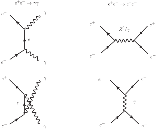
Figure 1: The lowest-order Feynman diagrams for the $\rm e^{+}e^{-}\rightarrow\gamma\gamma$ and $\rm e^{+}e^{-}\rightarrow e^{+}e^{-}$ reactions are shown. In the $\rm e^{+}e^{-}\rightarrow\gamma\gamma$ process, the reaction proceeds through the t- and u-channel. The Bhabha scattering $\rm e^{+}e^{-}\rightarrow e^{+}e^{-}$ proceeds through the s- and t-channel.

The two real photons in the final state of the $\rm e^{+}e^{-}\rightarrow\gamma\gamma$ reaction are indistinguishable, so the reaction proceeds through the t - and u - channels, while the s - channel is forbidden due to angular momentum conservation. The reaction is highly sensitive to long range QED interactions, and the two photons in the final state have left-handed and right-handed polarizations which results in total spin of zero, forbidding the s - channel with spin one for $\gamma$ and $Z^{0}$. As a pure annihilation reaction, the $e^{+}$ and $e^{-}$ in the initial state completely annihilate to two photons in the final state, making it easy to subtract the background signal.

The Bhabha reaction ${\rm e^{+}e^{-}\rightarrow e^{+}e^{-}}$ is a mixed reaction that occurs via scattering in both the s-channel and t-channel. At energies around the $Z^{0}$ pole, the $Z^{0}$ contribution dominates. The elastic scattering and annihilation channel are superimposed since the $e^{+}$ and $e^{-}$ in the initial and final states are identical. Therefore, the ${\rm e^{+}e^{-}\rightarrow e^{+}e^{-}}$ reaction serves as a test for the superimposition of short-range Weak Interaction and long-range QED interaction.

In this paper, we analyze deviations from QED by combining data on the differential cross section of the $\rm e^{+}e^{-}\rightarrow\gamma\gamma$ reaction measured by various $e^{+}e^{-}$ storage ring experiments. Specifically, the VENUS collaboration investigated this reaction in 1989 [50] at energies $\sqrt{s}$ = 55 GeV - 57 GeV, while the OPAL collaboration [51] studied it in 1991 at the $Z^{0}$ pole with $\sqrt{s}$ = 91 GeV. The TOPAS collaboration also investigated this reaction in 1992 at $\sqrt{s}$ = 57.6 GeV [52], while the ALEPH collaboration studied it in 1992 at the $Z^{0}$ pole with $\sqrt{s}$ = 91.0 GeV [53]. Moreover, the DELPHI collaboration investigated the reaction from 1994 to 2000 at energies ranging from $\sqrt{s}$ = 91.0 GeV to 202 GeV [54], while the L3 collaboration studied it from 1991 to 1993 at the $Z^{0}$ pole with center-of-mass energies ranging from $\sqrt{s}$ = 88.5 GeV to 93.7 GeV [55]. The L3 collaboration also studied the reaction in 2002 at center-of-mass energies ranging from $\sqrt{s}$ = 183 GeV to 207 GeV [56], and the OPAL collaboration investigated it in 2003 at center-of-mass energies ranging from $\sqrt{s}$ = 183 GeV to 207 GeV [59]. Deviations from QED were investigated through the study of contact interactions $e\ e\ \gamma\gamma$ and excited electron exchange displaced in the left panel of Fig. 1. Colleagues of some of the authors of this paper have reviewed experimental studies and models of deviations from QED in their thesis [60]. An earlier review is also available in [61].

The effective Lagrangian for a contact interaction is proportional to the lowest power of $1/\Lambda$, depending on the the dimensionality of the fields involved, and conserves helicity of fermion currents. This ensures known particle masses are much less than $\Lambda$. Different helicity choices for the fields used in the Lagrangian result in different predictions for angular distributions and polarization observables in reactions where the contact interaction is present. Figure 2b depicts the QED direct contact term, characterized by scale parameters $\Lambda_{+}$ and $\Lambda_{-}$. These parameters are subsequently interpreted as being indicative of an extended annihilation radius in the $\rm e^{+}e^{-}\rightarrow\gamma\gamma$ reaction. Figure 2c depicts Feynman diagrams that are sensitive to the mass of an excited electron, with the scale parameter $\Lambda_{e^{*}}$ being a function of $m_{e^{*}}$.

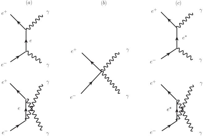
Figure 2: The lowest-order Feynman diagrams of the $\rm e^{+}e^{-}\rightarrow\gamma\gamma$ reaction are shown, with (a) representing QED, (b) contact interaction, and (c) excited electron exchange.

In 1989, the VENUS collaboration [50] established initial limits of $\Lambda_{+}>$ 81 GeV and $\Lambda_{-}>$ 82 GeV. Table 11 on page 186 of their publication provides an overview of other collaborations that have been studying the same subject. The significance of all analyses was below 1$\times\sigma$, and the fitted values of the parameters $1/\Lambda^{4}$ and $1/\Lambda_{e^{*}}^{4}$ were negative. In 2002, the L3 collaboration [56] established limits on $\Lambda_{+}>$ 400 GeV, $\Lambda_{-}>$ 300 GeV, and $m_{e^{*}}>$ 310 GeV, including negative fit parameters with a significance below 1$\times\sigma$. In their latest publication on the subject, in 2013 the LEP Electroweak Working Group [57] conducted an analysis of data from the differential cross section of all LEP detectors in the energy range of $\sqrt{s}$ = 133 GeV to 207 GeV. The group established limits of $\Lambda_{+}>$ 431 GeV, $\Lambda_{-}>$ 339 GeV, and $m_{e^{*}}>$ 366 GeV, which included negative fit parameters with a significance of nearly 2$\times\sigma$.

Thus, comparing the results obtained by combining the data from all LEP II collaborations with those from L3 alone, it can be observed that the increased statistics have led to more confident results. Based on this observation, we conduct a global fit using data from all six research projects mentioned above to investigate $\Lambda_{+}$, $\Lambda_{-}$, and $m_{e^{*}}$ for energies ranging from $\sqrt{s}$ = 55 GeV to 207 GeV, including the corresponding luminosities. An initial attempt to perform the global fit, which involved some of the authors of this paper, has been previously described in detail in [58]. It is noteworthy that the global fit revealed a significant deviation of the differential cross-section of the annihilation reaction $\rm e^{+}e^{-}\rightarrow\gamma\gamma$ from QED predictions, with a statistical significance of 5$\times\sigma$.

In the current paper, we scrutinize the global fitting procedure by examining all technical details used in the $\chi^{2}$ analysis. In Section 2, we provide a detailed description of the theoretical framework used for calculating the differential and total cross sections of the $\rm e^{+}e^{-}\rightarrow\gamma\gamma$ reaction in QED, including radiative corrections and modifications due to contact interactions and models with excited electrons. In Section 3, we present all the data used in the global fitting procedure, along with a description of the cross section measurement procedure. The $\chi^{2}$ analysis applied for the global fit is described in Section 4, and in Section 5, we validate our $\chi^{2}$ procedure by inferring the total cross section, which exhibits a similar significance of around 5$\times\sigma$. We discuss the systematic uncertainties of the analysis in Section 6. In Section 7, we interpret the results of the global fit in the context of the non-pointness of the electron and conclude.

2 Theoretical frameworks

The physical interactions in nature are governed by the principles of local gauge invariance, which are connected to conserved physical quantities of a local region of space. The Lagrangian formalism helps to establish the connection between symmetries and conservation laws.

The Dirac Lagrangian density describes a free particle of spin 1/2 as follows

$$\mathcal{L}_{\rm Dirac}=\overline{\Psi}(i\gamma^{\mu}\partial_{\mu}-m)\Psi,$$ (1)

where $\psi$ is the fermion field, $\bar{\psi}=\psi^{\dagger}\gamma^{0}$ is its adjoint spinor, $\gamma^{\mu}$ are the gamma matrices ($\gamma^{0}$ is a $4\times 4$ matrix, while $\gamma^{i}$ with $i=1,2,3$ are $4\times 4$ matrices), $\partial^{\mu}=\partial/\partial x^{\mu}$ is the derivative (with $x^{\mu}$ being a four-vector with dimensions of length), and $m$ is the mass of the particle. The requirement of local gauge invariance leads to the QED Lagrangian:

$${\mathcal{L}}_{\rm QED}=\overline{\Psi}(i\gamma^{\mu}\partial_{\mu}-m)\Psi+e\overline{\Psi}\gamma^{\mu}A_{\mu}\Psi-\frac{1}{4}F_{\mu\nu}F^{\mu\nu}\ ,$$ (2)

where $A_{\mu}$ is the gauge field, $m_{A}=m_{\gamma}=0$, $e$ is the electron charge, $e\overline{\Psi}\gamma^{\mu}A_{\mu}\Psi$ is the interaction term, and $F_{\mu\nu}=\partial_{\mu}A_{\nu}-\partial_{\nu}A_{\mu}$.

2.1 The lowest order cross section of ${\rm e^{+}e^{-}\rightarrow\gamma\gamma}$

The Born-level cross section [63, 79] of the ${\rm e^{+}e^{-}\rightarrow\gamma\gamma}$ reaction, also known as the leading-order cross section, is defined by the $\it{M}$-matrix given by

$$M_{fi}=-e\int\overline{\Psi}\gamma^{\mu}\Psi A_{\mu}d^{4}x\ ,$$ (3)

where $f$ and $i$ represent the final and initial states, respectively.

At high energies ($s\gg m_{e}^{2}$), the mass of the electron can be neglected. Thus, the differential cross section of the reaction depicted in Fig. 2a can be expressed as follows after averaging over the spin states of the initial particles:

$$\frac{d\sigma_{0}}{d\Omega}=\frac{S}{64\pi^{2}s}\frac{p_{f}}{p_{i}}\left|\it{M}\right|^{2}=\frac{\alpha^{2}}{s}\frac{1+\cos^{2}(\theta)}{k^{2}-\cos^{2}(\theta)}\ ,$$ (4)

where $\left|\it{M}\right|^{2}$ is the matrix element, $S=1/2$ is the statistical factor, $\sqrt{s}$ is the centre-of-mass energy of the $e^{+}e^{-}$ system, the momentum $p_{f}=p_{i}$ , $k=E_{e^{+}}/\left|\vec{p}_{e^{+}}\right|\simeq 1$ for high energies $E_{e^{+}}$ and $\alpha=e^{2}/4\pi$. The angle $\theta$ is the photon scattering angle with respect to the $e^{+}e^{-}$ - beam axis. The Born-level total cross section is expressed as

$$\sigma^{0} =\frac{1}{2!}\frac{\alpha^{2}}{s}\int_{0}^{2\pi}d\phi\int_{-1}^{+1}\frac{1+\cos^{2}\theta}{k-\cos^{2}\theta}d(\cos\theta)$$ (5)

$$=\frac{2\pi\alpha^{2}}{s}\left(\ln\left(\frac{s}{m^{2}_{e}}\right)-1\right)$$

.

As the statistics of the measurements of differential and total cross sections increases, it becomes essential to account for the radiative corrections discussed below.

2.2 Radiative corrections

In our analysis, we consider radiative corrections using a Monte Carlo method [63], which incorporates a complete third-order calculation that accounts for electron-mass effects.

The calculations involve six particles: the positron $e^{+}$ with momentum $p_{+}$, the electron $e^{-}$ with momentum $p_{-}$, virtual photons, and soft initial photons $\gamma(k_{3})$ with momentum $k_{3}$, as well as hard radiation photons $\gamma(k_{1})$ and $\gamma(k_{2})$ with momentum $k_{1}$ and $k_{2}$, respectively. The set of eight virtual photon corrections is illustrated by the Feynman graphs in Fig. 3. Fig. 4 shows the lowest order Feynman diagrams for two-photon annihilation and the set of corrections, consisting of six soft real photon initial state corrections and eight hard photon corrections [63].

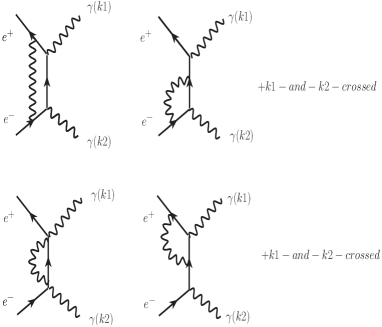
Figure 3: The figure shows the eight virtual photon corrections of third order Feynman graphs for the $\rm e^{+}e^{-}\rightarrow\gamma\gamma(\gamma)$ reaction. $k_{i}$ represents the momentum of the $i$-th photon.

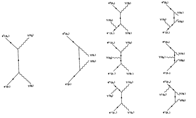
Figure 4: Feynman diagrams for two-photon annihilation and radiative corrections. The left side shows the lowest-order Feynman diagrams for two-photon annihilation. The right side shows the set of corrections, comprising of six soft initial state corrections for real photons, along with eight hard photon corrections. The diagrams are adapted from  [63]. In this figure, $q_{i}=k_{i}$ is the momentum of the $i$th photon.

As the exact analytical expression is not available, numerical simulations are used to calculate the corrections of the Feynman diagrams depicted in Figure 3 and Figure 4. For this purpose, an event generator [63] is employed to simulate the reaction $\rm e^{+}e^{-}\rightarrow\gamma\gamma(\gamma)$. The differential cross section, including radiative corrections up to $O(\alpha^{3})$, can be expressed as

$$\left(\frac{d\sigma}{d\Omega}\right)_{\alpha^{3}}=\left(\frac{d\sigma}{d\Omega}\right)_{\rm Born}(1+\delta_{\rm virtual}+\delta_{\rm soft}+\delta_{\rm hard})\ ,$$ (6)

where $\left(\frac{d\sigma}{d\Omega}\right)_{\rm Born}$ represents the lowest order cross section, while $\delta_{\rm virtual}$, $\delta_{\rm soft}$, and $\delta_{\rm hard}$ correspond to the virtual, soft-Bremsstrahlung, and hard-Bremsstrahlung corrections, respectively.

To differentiate between soft- and hard-Bremsstrahlung, we introduce a dimensionless discriminator $k_{0}\ll 1$ into the generator. If the momentum $k_{3}$ of the photon from initial state radiation (soft-Bremsstrahlung) satisfies $k_{3}/|p_{e^{+}}|<k_{0}$, the reaction is considered as 2-photon final state; otherwise, it is treated as 3-photon final state (hard-Bremsstrahlung). Here, $|p_{e^{+}}|$ represents the momentum of the positron $e^{+}$. To align with the notation used in (4), we use $p_{+}$ as a shorthand for $p_{e^{+}}$. The two cases are further elaborated in section 2.2.1 and 2.2.2.

2.2.1 Virtual and soft radiative corrections

If the energies of the photons from initial state radiation (soft Bremsstrahlung) are too small to be detected, i.e., $k_{3}/|p_{+}|<k_{0}$, the reaction is treated as a 2-photon final state process:

$$e^{+}(p_{+})+e^{-}(p_{-})\rightarrow\gamma(k_{1})+\gamma(k_{2})$$ (7)

Wherein, $\delta_{\rm virtual}+\delta_{\rm soft}$ are expresse as follows

$$\begin{matrix}\delta_{\rm soft}+\delta_{\rm virtual}=-\frac{\alpha}{\pi}\{2(1-2v)(\ln k_{0}+v)+\frac{3}{2}\vspace{0.2cm}\\ -\frac{1}{3}\pi^{2}+\frac{1}{2(1+\cos^{2}\theta)}\vspace{0.2cm}\\ \times[-4v^{2}(3-\cos^{2}\theta)-8v\cos^{2}\theta\\ +4uv(5+2\cos\theta+\cos^{2}\theta)\\ +4wv(5-2\cos\theta)+\cos^{2}\theta\\ -u(5-6\cos\theta+\cos^{2}\theta)\\ -w(5+6\cos\theta+\cos^{2})\\ -2u^{2}(5+2\cos\theta+\cos^{2}\theta)\\ -2w^{2}(5-2\cos\theta+\cos^{2}\theta)]\}\ ,\end{matrix}$$ (8)

where

$$v =\frac{1}{2}\ln\left(\frac{s}{m^{2}_{e}}\right)\ ,$$ (9)

$$u =\frac{1}{2}\ln\left(\frac{2(e+\cos\theta)}{m^{2}}\right)\ ,$$ (10)

$$w =\frac{1}{2}\ln\left(\frac{2(e-\cos\theta)}{m^{2}}\right)\ ,$$ (11)

$$m =\frac{m_{e}}{\left|p_{+}\right|}\quad\rm{and}\quad e=\frac{E_{e^{+}}}{\left|p_{+}\right|}.$$ (12)

Note that at low energy regime the expression above include the mass of the electron $m_{e}$.

The total cross section with two-$\gamma$s in the final state reads

$$\sigma^{2\gamma} =\sigma_{0}+\frac{2\alpha^{3}}{s}[2(2v-1)^{2}\ln k_{0}+\frac{4}{3}v^{3}+3v^{2}\vspace{0.2cm}$$ (13)

$$+(\frac{2}{3}\pi^{2}-6)v-\frac{1}{12}\pi^{2}].$$

2.2.2 Hard radiative corrections

If the energies of the photons from initial state radiation satisfy $k_{3}/|p_{+}|>k_{0}$, then the reaction is treated as a 3-photon final state process:

$$e^{+}(p_{+})+e^{-}(p_{-})\rightarrow\gamma(k_{1})+\gamma(k_{2})+\gamma(k_{3})\ .$$ (14)

To obtain the differential cross section of $\rm e^{+}e^{-}\rightarrow\gamma\gamma(\gamma)$, we need to introduce two additional parameters in the phase space. The computation (see [64] for details) is performed in the ultra-relativistic regime, which is as follows

$$\frac{d\sigma}{d\Gamma_{ijk}}=\frac{d\sigma}{d\Omega_{i}d\Omega_{k}dx_{k}}=\frac{\alpha^{3}}{8\pi^{2}s}w_{ijk}F(i,j,k)\ ,$$ (15)

where

$$w_{ijk} =\frac{x_{i}x_{k}}{y(z_{j})},x_{i}=\frac{k_{i0}}{\left|\vec{p_{+}}\right|}\ ,$$ (16)

$$y(z_{j}) =2e-x_{k}+x_{k}z_{j}\ ,$$ (17)

$$z_{j} =cos(\alpha_{ik})\ ,$$ (18)

$$x_{l} =\frac{E_{l}}{\left|\vec{p_{+}}\right|}\ ,$$ (19)

$$F(i,j,k) =\sum_{p}\left[-2m^{2}\frac{{k_{j}}^{\prime}}{k^{2}_{k}{k_{i}}^{\prime}}-2m^{2}\frac{k_{j}}{{k}^{\prime 2}_{k}k_{i}}+\frac{2}{k_{k}{k}^{\prime}_{k}}\left(\frac{k^{2}_{j}+{k}^{\prime 2}_{j}}{k_{i}{k}^{\prime}_{i}}\right)\right]$$

$$=\sum_{p}M(i,j,k)$$ (20)

and $\alpha_{ik}$ is the angle between $k_{i}$ and $k_{j}$. $P$ binds all permutations of ( 1, 2, 3 ). The quantities $k_{i}$ and $k^{\prime}_{i}$ are give by

$$k_{i} =x_{i}(e-\cos(\theta_{i}))$$ (21)

end

$${k}^{\prime}_{i} =x_{i}(e+\cos(\theta_{i}))$$ (22)

respectively, where $\theta_{i}$ is the angle between the momentum of the i-th photon and $|\vec{p}_{+}|$.

In its turn, the total cross section with three-$\gamma$s in the final state reads

$$\sigma^{3\gamma}=\frac{1}{3!}\int d\Gamma_{ijk},i,j,k\in{\{1,2,3\}},$$ (23)

where the integral runs over the phase spaces defined by $k_{0}<x_{i}<1$. In practice, (23) can be approximated by an analytical expression in which the photons are sorted by their energies, such that $E_{\gamma 1}\geq E_{\gamma 2}\geq E_{\gamma 3}$. Here, $\gamma_{1}$ and $\gamma_{2}$ are treated as annihilation photons, and $\gamma_{3}$ is treated as a hard Bremsstrahlung photon. Integrating (23) (performed in [63]) one arrives to

$$\sigma^{3\gamma}=\frac{2\alpha^{3}}{s}[3-(\ln\frac{4}{m^{2}}-1)^{2}(2\ln k_{0}+1)].$$ (24)

2.3 The total cross section in $\rm e^{+}e^{-}\rightarrow\gamma\gamma(\gamma)$

The total cross section for $\rm e^{+}e^{-}\rightarrow\gamma\gamma(\gamma)$ is obtained by summing (13) and (24), given by

$$\sigma_{tot} =\sigma(2\gamma)+\sigma(3\gamma)$$ (25)

$$=\sigma^{0}+\frac{2\alpha^{3}}{s}[\frac{4}{3}v^{3}-v^{2}+(\frac{2}{3}\pi^{2}-2)v+2-\frac{1}{12}\pi^{2}].$$ (26)

2.4 The numerical calculation of the $\rm e^{+}e^{-}\rightarrow\gamma\gamma(\gamma)$ differential cross section

The third-order differential cross-section is obtained using a Monte Carlo generator [63]. The generator produces events with three photons sorted in descending order of their energies ($E_{\gamma 1}\geq E_{\gamma 2}\geq E_{\gamma 3}$) and at an angle $\alpha$ between photons with energies $E_{\gamma 1}$ and $E_{\gamma 2}$, with the correct mixture of soft ($k_{3}/|p_{+}|<k_{0}$) and hard QED corrections ($k_{3}/|p_{+}|>k_{0}$), as shown in Fig 3 and Fig 4. The gamma event acceptance range is defined by $\alpha_{min}<\alpha<\alpha_{max}$. The angle $\alpha$ is analytically related to the scattering angle $\theta$, thus connecting the limits to $|cos\theta|$.

The differential cross section is calculated as

$$\overline{(\frac{d\sigma}{d\Omega})}_{i}=\frac{1}{2\pi\Delta(|\cos\theta|)}\sigma_{\rm tot}\frac{N_{i}}{N}\ ,$$ (27)

where $|cos\theta|=(|\cos\theta_{1}|+|\cos\theta_{2}|)/2$ is the scattering angle, with $\theta_{1}$ and $\theta_{2}$ being the scattering angles of $E_{\gamma 1}$ and $E_{\gamma 2}$, respectively. $N_{i}$ is the number of events in an angular bin width $\Delta(|cos\theta|)$, and $N$ is the total number of generated events.

To search for potential deviations from QED, the generated cross section (27) is fitted as a function of $|\cos\theta|$ using a 6-parameter $\chi^{2}$ fit for each center-of-mass energy $E_{\rm tot}$ analyzed.

As an illustration, we generated one million events at a center-of-mass energy of 189 GeV, within an acceptance range of $14^{\circ}<\alpha<166^{\circ}$, which corresponds to the scattering angle range of $|\cos\theta|<0.97$. We used a soft/hard discriminator of $k_{0}=0.01$ and distributed the events over 50 $\Delta(|\cos\theta|)$ bins. The resulting $\chi^{2}$ of the differential cross section exhibits the following polynomial behavior

$$\left(\frac{d\sigma}{d\Omega}\right)_{\rm QED}=\left(\frac{d\sigma}{d\Omega}\right)_{\rm Born}\times$$ (28)

$$\left(1+p_{1}+p_{2}e^{-\frac{x^{1.2}}{2p^{2}_{3}}}+p_{4}x+p_{5}x^{2}+p_{6}x^{3}\right)\ ,$$

where $x=|\cos\theta|$ and

$$p_{1} =0.2869\ ,$$ (29)

$$p_{2} =-0.51851\ ,$$

$$p_{3} =0.19946\ ,$$

$$p_{4} =-0.39652\ ,$$

$$p_{5} =-0.41213\ ,$$

$$p_{6} =0.70428.$$

We note, that $\rm e^{+}e^{-}\rightarrow\gamma\gamma(\gamma)$ channel lacks a comprehensive analysis of theoretical uncertainty, specifically the uncertainty associated with the third-order Monte Carlo prediction. In a QED process, higher-order effects can be approximated to be 10% ($\simeq\sqrt{\alpha}$) of the correction caused by the highest order corrections. The theory uncertainty can be estimated to be 10% of the radiative correction for each experiment, with a minimum of 0.5%.

2.5 Deviations from QED

If QED is a fundamental theory, it should be capable of describing the experimental parameters of the $\rm e^{+}e^{-}\rightarrow\gamma\gamma(\gamma)$ reaction up to the Grand Unification scale. However, currently, QED has only been tested up to $E\lesssim 100$ GeV. Therefore, at higher energy scales, new non-QED phenomena may become observable. If an energy scale characterized by a cutoff parameter $\Lambda$ is found, it can serve as a threshold point for the breakdown of QED and the emergence of new underlying physics. This paper focuses on the mass of the excited electron and the scale of the contact interaction, which can be interpreted in terms of the size of the electron.

2.5.1 Heavy electron mass

This model assumes the existence of an excited state of the electron, and the reaction $\rm e^{+}e^{-}\rightarrow\gamma\gamma$ occurs through the exchange of a virtual excited electron $e^{*}$ in the t- and u-channel, as depicted in the Feynman graph in Fig. 2c. The interaction is characterized by a coupling between the excited electron and the ordinary electron, as well as between the excited electron and the photon. A magnetic interaction term [43, 68] is introduced to account for this interaction in the form

$${\mathcal{L}}_{e^{*}}=\frac{e\lambda}{2m_{e^{*}}}\overline{\Psi}_{e^{*}}\sigma_{\mu\nu}\Psi_{e}F^{\mu\nu}\ ,$$ (30)

where $\lambda$ is the relative magnetic coupling strength to the QED magnetic coupling, $m_{e^{*}}$ the mass of the excited electron and $\sigma^{\mu\nu}=\frac{1}{2}\left[\gamma^{\mu},\gamma^{\nu}\right]$. The QED differential cross section modified by this interaction reads

$$\frac{d\sigma}{d\Omega}=\left(\frac{d\sigma}{d\Omega}\right)_{QED}\left[1+\frac{s^{2}}{2}\frac{\lambda^{2}}{m^{4}_{e^{*}}}\left(1-\cos^{2}\theta\right)F(\cos\theta)\right]\ ,$$ (31)

where $\sqrt{s}$ is the centre-of-mass energy and $F(\cos\theta)$ is given by

$$F(\cos\theta)= \left(1+\frac{s}{2m^{2}_{e^{*}}}\frac{1-\cos^{2}\theta}{1+\cos^{2}\theta}\right)\times$$ (32)

$$\left[\left(1+\frac{s}{2m^{2}_{e^{*}}}\right)^{2}-\left(\frac{s}{2m^{2}_{e^{*}}}\right)^{2}\cos^{2}\theta\right]^{-1}.$$

At condition $s/m^{2}_{e^{2}}<<1$ the expression for the differential cross section (31) is reduced to

$$\frac{d\sigma}{d\Omega} =\left(\frac{d\sigma}{d\Omega}\right)_{QED}(1\pm\delta_{new})$$ (33)

$$=\left(\frac{d\sigma}{d\Omega}\right)_{QED}\left[1\pm\frac{s^{2}}{2}\frac{1}{\Lambda^{4}_{\pm}}(1-\cos^{2}\theta)\right]\ ,$$

where the scale $\Lambda_{+}=\Lambda_{e^{*}}$ is related to the mass of the excited electron $m_{e^{*}}$ by $\Lambda^{2}_{+}=m^{2}_{e^{*}}/\lambda$ and negative contribution $\Lambda_{-}$ is added for symmetry.

2.5.2 Minimal interaction length and non-pointness of the electron

The effective Lagrangian for a contact interaction uses current fields of known particles and is proportional to the lowest power of $1/\Lambda$, which depends on the dimensionality of the fields used. When constructing this Lagrangian, it is important to ensure that fermion currents conserve helicity, which is necessary for composite models. This condition ensures that known particle masses are much less than the energy scale $\Lambda$. Different choices of helicity for the fields used in the Lagrangian result in different predictions for the angular distributions and polarization observables in reactions where the contribution of the contact interaction is considered.

In [65, 66, 67], the contact interaction between two fermions and two bosons was studied in a general case. In the following discussion, we will focus on the simplest dimension-6 operator, which is described by the effective Lagrangian

$${\mathcal{L}}_{6}=i\overline{\Psi}\gamma_{\mu}({\vec{D}}_{\nu}\Psi)(g_{6}F^{\mu\nu}+\tilde{g}_{6}\tilde{F}^{\mu\nu})\ ,$$ (34)

where coupling constant $g_{n}$, where $n=6$, is related to the mass scale $\Lambda$ by $g_{n}=\sqrt{4\pi}/\Lambda^{(n-4)}$. The QED covariant derivative is represented by $D_{\mu}=\partial{\mu}-ieA{\mu}$, and the dual of the electromagnetic tensor is $\tilde{F}^{\mu\nu}$, given by $\tilde{F}^{\alpha\beta}=\frac{1}{2}\varepsilon^{\alpha\beta\mu\nu}F_{\mu\nu}$. The modified differential cross section reads

$$\left(\frac{d\sigma}{d\Omega}\right)_{T} =\left(\frac{d\sigma}{d\Omega}\right)_{QED}\left[1\pm\delta_{\rm new}\right]$$ (35)

$$=\left(\frac{d\sigma}{d\Omega}\right)_{QED}\left[1\pm\frac{s^{2}}{2\alpha}\left(\frac{1}{\Lambda^{4}}+\frac{1}{\tilde{\Lambda^{4}}}\right)(1-\cos^{2}\theta)\right]\ ,$$

where we use $\Lambda=\tilde{\Lambda}=\Lambda_{6}$, and omit higher order terms such as $\Lambda_{7}$ or $\Lambda_{8}$ in $\delta_{\rm new}$.

A common method for searching for deviations from QED is to use a $\chi^{2}$ test to compare experimentally measured cross sections with predicted QED cross sections. To incorporate a non-QED direct contact term into the QED cross section, an energy scale $\Lambda$ is introduced via Equation (35). This $\Lambda$ can be interpreted as defining the size of the object where annihilation occurs, which can be calculated using either the generalized uncertainty principle [69, 70, 71] or the electromagnetic energy $E$ and wavelength $\lambda_{\gamma}$ [72] of the light emitted by the object. The wavelength $\lambda_{\gamma}$ must be smaller or equal to the size of the interaction area. If the $\chi^{2}$ test exhibits a minimum for a certain energy scale $\Lambda$, it defines the region in which $e^{+}e^{-}$ annihilation must occur via $\Lambda=E=\hbar\times\nu_{\gamma}$ and $\nu_{\gamma}\times\lambda_{\gamma}=c$. We assume that $\lambda_{\gamma}=r_{e}$ regulates the size of the electron according to

$$r_{e}=\frac{\hbar c}{\Lambda}\ ,$$ (36)

which includes the Planck constant $\hbar$ and the speed of light $c$.

Equation (36) provides a generic formula for calculating the size of an object, which can be obtained using the generalized uncertainty principle [74, 75]. It is worth noting that as $\Lambda$ approaches infinity in Equation (36), the size of the object will tend to zero, i.e., $r_{e}\rightarrow 0$.

3 The measurement of the total and differential cross section

The $\rm e^{+}e^{-}\rightarrow\gamma\gamma(\gamma)$ reaction initiates in a storage $e^{+}e^{-}$ ring accelerators a background free signal in a detector. For example, Fig. 5 shows a typical event display captured in the central detector’s cross section of the L3 detector at LEP, providing a representation of the signal appearance. Similar signals have been observed in all LEP detectors, as well as in VENUS and TOPAS detectors. The channel’s topology is clean and the event selection is based on the presence of two energetic clusters in the ECAL. As The two highest-energy clusters must meet a minimum energy requirement. The cuts on acollinearity, or missing longitudinal momentum, as well as the allowed range in polar angle, of the observed clusters, have been applied. Charged tracks are generally not allowed, except when they can be associated with a photon conversion in one hemisphere, in order to remove background, particularly from Bhabha events.

The limited coverage of the ECAL, along with selection cuts to reject events with charged tracks, reduces the signal efficiency. The impact of the above mentioned cuts varies significantly depending on the detector geometry, resulting in uncorrelated systematic errors across LEP experiments, VENUS and TOPAS.

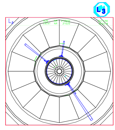
Figure 5: The event display of an $\rm e^{+}e^{-}\rightarrow\gamma\gamma(\gamma)$ event captured in the L3 detector at LEP, courtesy from [76].

The total cross section is calculated as the ratio of the number of detected events $N$ within the full angular coverage of the ECAL to the efficiency $\varepsilon$ and the integrated luminosity $L$

$$\sigma_{\rm tot}=\frac{N}{\varepsilon L}.$$ (37)

The differential cross section is calculated as

$$\overline{\left(\frac{d\sigma}{d\Omega}\right)}_{i}=\frac{1}{2\pi\Delta(|\cos\theta|)_{i}}\cdot\frac{N_{i}}{L\cdot\epsilon_{i}},$$ (38)

where $N_{i}$ is the number of events detected within an angular bin $i$ and $\varepsilon_{i}$ is the efficiency defined in the same angular bin. To compare the measured differential cross section given in (38) with QED predictions in the $i$th bin, the average value of $\cos\theta$ is calculates as

$$\left|\cos\theta\right|_{i}=\frac{\int_{|\cos\theta|\in i}|\cos\theta|\cdot\left(\frac{d\sigma}{d\Omega}(|\cos\theta|)\right)_{e^{+}e^{-}\rightarrow\gamma\gamma}^{\rm Born}\cdot d|\cos\theta|}{\int_{|\cos\theta|\in i}\left(\frac{d\sigma}{d\Omega}(|\cos\theta|)\right)_{e^{+}e^{-}\rightarrow\gamma\gamma}^{\rm Born}\cdot d|\cos\theta|}.$$ (39)

Here, $\cos\theta$ is defined as $0.5*||\cos\theta_{1}|+|\cos\theta_{2}||$, where $\cos\theta_{1}$ and $\cos\theta_{2}$ are the scattering angles of the first and second photon, respectively. The average calculation is based on the QED Born-level prediction. The collaborations present their data in bins of $\left|\cos\theta\right|_{i}$ where the cross section is calculated based on the number of events in each bin. Therefore, each value of $\left|\cos\theta\right|_{i}$ corresponds to the low edge of the bin.

3.1 Differential cross section data sets

This section describes the data on the differential cross section of the reaction $\rm e^{+}e^{-}\rightarrow\gamma\gamma$ that are included in the global fit analysis. The data is reweighted for a single center-of-mass energy $E_{\rm scale}$ and presented by plotting the reweighted results along with the QED-$\alpha^{3}$ cross section (6). Since the measurements of the cross section are obtained with varying event numbers $N_{i}$ and at different center-of-mass energies $E_{i}$, the reweighting is necessary to enable the visual comparison of different data sets. This is illustrated in Fig. 6 - 11. The reweighting is performed using the equation

$$\left(\frac{d\sigma}{d\Omega}\right)_{|\cos\theta|_{j}}^{\rm scale}=\frac{\sum_{i}^{r}N_{i}\left(\frac{d\sigma}{d\Omega}\right)^{i}_{|\cos\theta|_{j}}\cdot\left(\frac{E_{i}}{E_{\rm scale}}\right)^{2}}{\sum_{i}^{r}N_{i}}\ .$$ (40)

In this equation, $N_{i}$ is used to derive the differential cross section at center-of-mass energy $E_{i}$, where $i$ runs from 1 to $r$, which represents the number of differential cross section results ($\left(\frac{d\sigma}{d\Omega}\right)^{i}{|\cos\theta|{j}}$) to be scaled. Here, $j$ is the $\cos\theta$ bin number, and $\cos\theta_{j}$ is calculated using equation (39). The plots Fig. 6 - 11 are obtained with $E_{\rm scale}=91.2$ GeV. A potential deviation from QED in the differential cross section of the $\rm e^{+}e^{-}\rightarrow\gamma\gamma$ reaction would manifest as an observation of a difference between the QED and experimental differential cross sections.

The VENUS collaboration presented the luminosity, ${\rm e^{+}e^{-}\rightarrow\gamma\gamma}$ candidates, angular distribution, and differential cross section at four center-of-mass energies ($\sqrt{s}$ = 55.0 GeV, 56.0 GeV, 56.5 GeV and 57.6 GeV) in Tables 2-4 and 8 of [50]. The TOPAS collaboration presented the luminosity and differential cross section with bin width at a single center-of-mass energy ($\sqrt{s}$ = 57.0 GeV) in Tables 1 and 2 of [52]. Fig. 6 displays the reweighted data from VENUS and TOPAS, obtained using (40) with $E_{\rm scale}=91.2$ GeV, alongside the QED-$\alpha^{3}$ differential cross section at $\sqrt{s}$ = 91.2 GeV as a black line, with statistical uncertainties shown.

Figure 6: The differential cross section of the $\rm e^{+}e^{-}\rightarrow\gamma\gamma$ reaction from VENUS and TOPAS is presented, along with their statistical uncertainties. The black line is the QED-$\alpha^{3}$ cross section (6). The plot is obtained with $E_{\rm scale}=91.2$ GeV. A potential deviation from QED in the differential cross section of the $\rm e^{+}e^{-}\rightarrow\gamma\gamma$ reaction would manifest as an observation of a difference between the QED and experimental differential cross sections.

The ALEPH collaboration provided data on the differential cross section at $\sqrt{s}=91.3$ GeV, as well as the bin width, in Table 8.2 of [53]. The luminosity is reported on page 321 of [53]. Fig. 7 shows the ALEPH data scaled to $\sqrt{s}=91.2$ GeV using equation (40). Only statistical uncertainties are displayed. The black line corresponds to the QED-$\alpha^{3}$ differential cross section at $\sqrt{s}=91.2$ GeV.

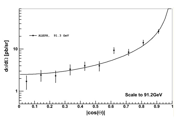
Figure 7: Same plot as shown in Fig. 6, but obtained from the ALEPH collaboration.

The DELPHI collaboration published data in [54] from 1994, 1998, and 2000. The 1994 results in Table 1 show the luminosity at $\sqrt{s}$ = 91.25 GeV and in Table 2 the differential $\rm e^{+}e^{-}\rightarrow\gamma\gamma$ cross section, together with the bin width and number of events per bin. The 1998 results in Table 2 show the luminosities of $\rm e^{+}e^{-}\rightarrow\gamma\gamma$ reaction, the number of events at different energies, and in Table 3 the differential cross section at different energies ($\sqrt{s}$ = 91.25 GeV, 130.4 GeV, 136.3 GeV, 161.5 GeV 172.4 GeV and 182.7 GeV) together with the bin width and number of events per bin. In 2000 results on page 71, the luminosity and differential cross section at different energies ($\sqrt{s}$ = 188.63 GeV, 191.6 GeV, 195.5 GeV, 199.5 GeV and 201.6 GeV) are shown in Table 3. Fig. 8 displays the DELPHI data scaled with (40) to $\sqrt{s}$ = 91.2 GeV. The black line represents the QED-$\alpha^{3}$ differential cross section at $\sqrt{s}$ = 91.2 GeV, and only statistical uncertainties are shown.

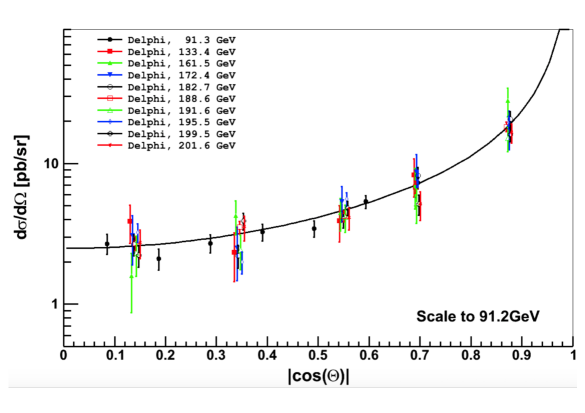
Figure 8: Same plot as shown in Fig. 6, but obtained from the DELPHI collaboration.

In 1995, L3 collaboration published data [55] on $\sqrt{s}$ = 91.2 GeV. The luminosity is displayed on page 141 and the differential cross section is shown in Table 1 with bin size and event counts. The 2000 data [62] includes luminosity for $\sqrt{s}$ = 183 GeV and $\sqrt{s}$ = 189 GeV on page 201. The 2002 data [56] includes luminosity for $\sqrt{s}$ = 192 GeV, 196 GeV, 200 GeV, 202 GeV, 205 GeV, and 207 GeV in Table 1. Table 4 shows the data events per efficiency and bin size for all energies of the 2000 and 2002 data. Figure 9 displays all L3 differential cross section data from $\sqrt{s}$ = 91 GeV to 207 GeV, scaled with (40) to 91.2 GeV. Only statistical uncertainties are shown. The black line represents the QED-$\alpha^{3}$ differential cross section at $\sqrt{s}$ = 91.2 GeV.

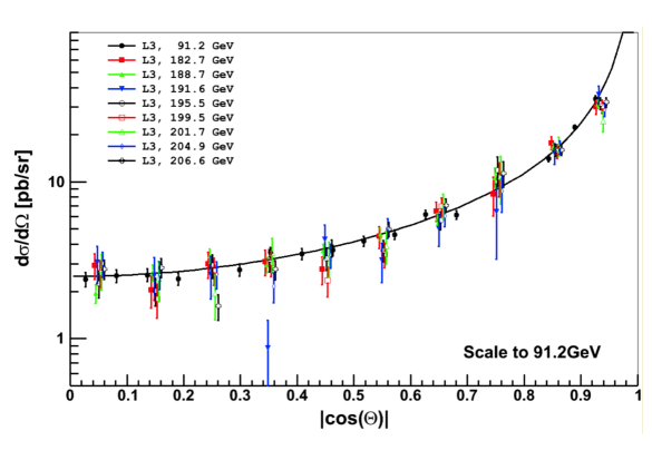
Figure 9: Same plot as shown in Fig. 6, but obtained from the L3 collaboration.

The OPAL collaboration published data for $\sqrt{s}$ = 91.0 GeV in 1991 [51], including luminosity on page 533, and differential cross section with number of events and bin size in Table 3. In 2003 [59], data for $\sqrt{s}$ = 183 GeV, 189 GeV, 192 GeV, 196 GeV, 200‘GeV, 202 GeV, 205 GeV and 207 GeV were published in Table 6 with number of events per bin, bin size, and efficiency. Figure 10 displays all the OPAL differential cross section data from $\sqrt{s}$ = 91 GeV to 207 GeV, scaled with (40) to 91.2 GeV, with only statistical uncertainties displayed. The black line is the QED-$\alpha^{3}$ differential cross section at $\sqrt{s}$ = 91.2 GeV.

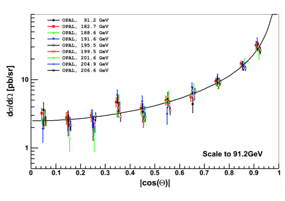
Figure 10: Same plot as shown in Fig. 6, but obtained from the OPAL collaboration.

Fig. 11 summarises the differential cross sections measured by VENUS, TOPAS, ALEPH, L3, and OPAL at energies ranging from $\sqrt{s}$ = 55 GeV to 207 GeV. All data points are scaled with (40) to 91.2 GeV and only statistical uncertainties are displayed. The black line represents the QED-$\alpha^{3}$ differential cross section at $\sqrt{s}$ = 91.2 GeV.

No significant deviations from QED predictions are visible in Fig. 6 - 11. In the following section, we will perform a global $\chi^{2}$ fit to the combined dataset.

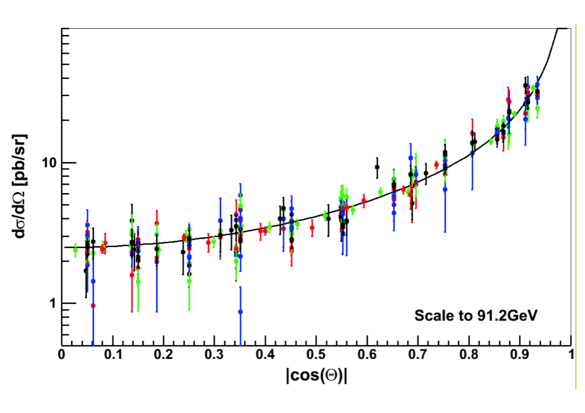
Figure 11: Differential cross section of the $\rm e^{+}e^{-}\rightarrow\gamma\gamma$ reaction from VENUS, TOPAS, ALEPH. L3 and OPAL. The black line is the QED $\alpha^{3}$ cross section (6). The colours and symbols are defined in Fig. 6 to 10.

Table 1: The integrated luminosity used from the VENUS, TOPAS, ALEPH, DELPHI, L3 and OPAL experiment.

GeV	VENUS	TOPAS	ALEPH	DELPHI	L3	OPAL
$55$	2.34 $pb^{-1}$ [50]
$56$	5.18 $pb^{-1}$ [50]
$56.5$	0.86 $pb^{-1}$ [50]
$57$	3.70 $pb^{-1}$ [50]
$57.6$		52.26 $pb^{-1}$ [52]
$91$			8.5 $pb^{-1}$ [53]	36.9 $pb^{-1}$ [54]	64.6 $pb^{-1}$ [55]	7.2 $pb^{-1}$ [51]
$133$				5.92 $pb^{-1}$ [54]
$162$				9.58 $pb^{-1}$ [54]
$172$				9.80 $pb^{-1}$ [54]
$183$				52.9 $pb^{-1}$ [54]	54.8 $pb^{-1}$ [56]	55.6 $pb^{-1}$ [59]
$189$				151.9 $pb^{-1}$ [54]	175.3$pb^{-1}$ [56]	181.1 $pb^{-1}$ [59]
$192$				25.1$pb^{-1}$ [54]	28.8 $pb^{-1}$ [56]	29.0 $pb^{-1}$ [59]
$196$				76.1 $pb^{-1}$ [54]	82.4$pb^{-1}$ [56]	75.9 $pb^{-1}$ [59]
$200$				82.6 $pb^{-1}$ [54]	67.5 $pb^{-1}$ [56]	78.2 $pb^{-1}$ [59]
$202$				40.1 $pb^{-1}$ [54]	35.9 $pb^{-1}$ [56]	36.8 $pb^{-1}$ [59]
$205$					74.3 $pb^{-1}$ [56]	79.2 $pb^{-1}$ [59]
$207$					138.1 $pb^{-1}$ [56]	136.5 $pb^{-1}$ [59]

4 Global $\chi^{2}$ test of the differential cross section

The non-QED model parameters discussed in Section 2.5 are determined by applying a $\chi^{2}$ test to the combined differential cross-section data measured by VENUS, TOPAS, OPAL, DELPHI, ALEPH, and L3 collaborations. The following expression is minimized using the MINUIT [78] code from CERNLIB for the $\chi^{2}$ test

$$\chi^{2}=\sum_{i,j}\left\{\frac{\frac{d\sigma}{d\Omega}^{\rm meas}(|\cos\theta|_{i},E_{j})-\frac{d\sigma}{d\Omega}^{new}(|\cos\theta|_{i},E_{j},\Lambda)}{\Delta\left[\frac{d\sigma}{d\Omega}^{\rm meas}(|\cos\theta|_{i},E_{j})\right]}\right\}^{2}.$$ (41)

Here, $\frac{d\sigma}{d\Omega}^{meas}(|\cos\theta|_{i},E_{j})$ is the measured differential cross section at an angular bin ($i$) and a center-of-mass energy ($j$), while $\frac{d\sigma}{d\Omega}^{new}(|\cos\theta|i,E_{j},\Lambda)$ is the $QED-\alpha^{3}$ differential cross section at an angular bin ($i$), a center-of-mass energy ($j$) and a test parameter $\Lambda$, as defined in equations (33) and (35). The ($\pm$) sign in front of $\delta_{\rm new}$ in equations (33) and (35) allows the $\chi^{2}$ test to search for positive and negative interference. The term $\Delta\left[\frac{d\sigma}{d\Omega}^{meas}(|\cos\theta|_{i},E_{j})\right]$ is the uncertainty of the mean value of the measurements, which is represented by sum in quadraturs of the statistical and systematic uncertainty (to be discussed in Chapter 6). The $\chi^{2}$ test requires details of the differential cross section and the luminosity at the different center-of-mass energies at which the data were taken. The previous section provided a description of the data set utilized in the analysis, which included individual sub-sets published by the collaborations. Table 1 provides a summary of the luminosities for all sub-sets from VENUS, TOPAS, ALEPH, DELPHI, L3, and OPAL that were used in the $\chi^{2}$ test.

4.1 Global $\chi^{2}$ test for heavy electron $m_{e*}$

In order to perform the $\chi^{2}$ fit in equation (41), it is necessary to use the differential QED cross section (28) for a given center-of-mass energy, as well as the differential cross section calculated for the heavy electron (31) and (32). The $\chi^{2}$ fit can be performed separately for every data sub-set at respective $\sqrt{s}$ by either utilizing the experimentally measured differential cross section if available, or calculating it using the luminosity, number of events per angular bin width and efficiency, as described in equations (38) and (39). The theoretical QED-$\alpha^{3}$ differential cross section is computed using the numerical calculations of the $\rm e^{+}e^{-}\rightarrow\gamma\gamma(\gamma)$ reaction discussed in section 2.4. The parameter $1/\Lambda_{+}^{4}$ is used in the cross section (33) for the test. Table 2 displays the resulting fit parameters ($1/\Lambda_{+}^{4}$ in $1/\mathrm{GeV}^{4}$) and fit quality parameter $\chi^{2}/dof$ of the $\chi^{2}$ test for every data sub-set. The table is sorted by $\sqrt{s}$ value and collaboration.

Table 2: The fit parameter $1/\Lambda_{+}^{4}$ in units of $1/{\rm GeV}^{4}$ for each data sub-set, along with the corresponding fit quality parameter $\chi^{2}/{\rm dof}$, attributed $\sqrt{s}$ values, and collaboration name.

GeV	$VENUS\ (\chi^{2}/dof)$	$TOPAS$	$ALEPH$	$DELPHI$	$L3$	$OPAL$
$55$	$-(4.26\pm 2.52)\times 10^{-8}$
	$\chi^{2}/dof=12.90/8$
$56$	$(3.24\pm 1.88)\times 10^{-8}$
	$\chi^{2}/dof=9.48/8$
$56.5$	$-(2.11\pm 3.96)\times 10^{-8}$
	$\chi^{2}/dof=4.93/8$
$57$	$-(1.49\pm 2.02)\times 10^{-8}$
	$\chi^{2}/dof=8.82/8$
$57.6$		$-(1.59\pm 5.61)\times 10^{-9}$
		$\chi^{2}/dof=7.32/5$
$91$			$(0.07\pm 2.98)\times 10^{-9}$	$-(2.29\pm 1.70)\times 10^{-9}$	$-(6.88\pm 8.00)\times 10^{-10}$	$-(0.93\pm 3.59)\times 10^{-9}$
			$\chi^{2}/dof=9.96/9$	$\chi^{2}/dof=3.54/6$	$\chi^{2}/dof=11.1/15$	$\chi^{2}/dof=6.92/8$
$133$				$-(0.48\pm 1.26)\times 10^{-9}$
				$\chi^{2}/dof=2.60/3$
$162$				$-(2.35\pm 5.40)\times 10^{-10}$
				$\chi^{2}/dof=4.59/4$
$172$				$(0.74\pm 5.19)\times 10^{-10}$
				$\chi^{2}/dof=1.09/4$
$183$				$-(2.54\pm 1.60)\times 10^{-10}$	$-(1.48\pm 1.37)\times 10^{-10}$	$(2.05\pm 1.43)\times 10^{-10}$
				$\chi^{2}/dof=5.27/4$	$\chi^{2}/dof=11.0/9$	$\chi^{2}/dof=5.86/9$
$189$				$(0.14\pm 1.01)\times 10^{-10}$	$-(8.58\pm 7.16)\times 10^{-11}$	$-(2.05\pm 6.89)\times 10^{-11}$
				$\chi^{2}/dof=2.67/4$	$\chi^{2}/dof=17.2/9$	$\chi^{2}/dof=5.13/9$
$192$				$-(3.95\pm 2.07)\times 10^{-10}$	$-(5.79\pm 1.41)\times 10^{-10}$	$(0.31\pm 1.63)\times 10^{-10}$
				$\chi^{2}/dof=1.03/4$	$\chi^{2}/dof=16.9/9$	$\chi^{2}/dof=12.6/9$
$196$				$-(0.43\pm 1.19)\times 10^{-10}$	$-(1.93\pm 0.89)\times 10^{-10}$	$-(1.62\pm 9.37)\times 10^{-11}$
				$\chi^{2}/dof=16.4/4$	$\chi^{2}/dof=7.84/9$	$\chi^{2}/dof=7.48/9$
$200$				$-(0.88\pm 1.12)\times 10^{-10}$	$-(2.58\pm 0.90)\times 10^{-10}$	$-(1.65\pm 0.84)\times 10^{-10}$
				$\chi^{2}/dof=8.07/4$	$\chi^{2}/dof=13.8/9$	$\chi^{2}/dof=8.63/9$
$202$				$-(1.11\pm 1.51)\times 10^{-10}$	$-(1.49\pm 1.24)\times 10^{-10}$	$-(1.47\pm 1.16)\times 10^{-10}$
				$\chi^{2}/dof=2.94/4$	$\chi^{2}/dof=15.2/9$	$\chi^{2}/dof=17.8/9$
$205$					$-(1.07\pm 0.84)\times 10^{-10}$	$-(3.81\pm 7.99)\times 10^{-11}$
					$\chi^{2}/dof=12.9/9$	$\chi^{2}/dof=6.26/9$
$207$					$-(9.14\pm 5.99)\times 10^{-11}$	$-(1.52\pm 0.57)\times 10^{-10}$
					$\chi^{2}/dof=23.6/9$	$\chi^{2}/dof=10.7/9$

About 80% of the data sub-sets in Table 2 exhibit a preference for negative values of $1/\Lambda_{+}^{4}$. This trend is also evident in Fig. 12 and Table 3. Figure 12 displays the results of the $\chi^{2}$ tests for the data sub-sets, grouped according to their collaborations (ALEPH, Delphi, L3, OPAL), and combinations of collaborations such as TRISTAN (TOPAS and VENUS), LEP 1, and LEP 2. The trend towards negative values of $1/\Lambda_{+}^{4}$ becomes more pronounced as the statistics of the grouped combinations increases.

Table 3 shows the values of $1/\Lambda^{4}$ in units of GeV^-4 obtained from the fits to data combined in groups of collaborations. For TRISTAN, the values are positive with the large error bar for energies ranging from $\sqrt{s}=55$ GeV to 57.6 GeV. At LEP 1, where the data were taken at the $Z^{0}$ pole with lower luminosity, the values are already negative with a statistical significance of approximately one standard deviation. This is reflected in the size of the error bars in Table 3. The LEP 2 data, covering energies from 133 GeV to 207 GeV, have much higher luminosity and dominate the global fit result. The fitted parameter is negative with a significance of approximately five standard deviations in this energy range. Note that the $\chi^{2}$ distribution exhibits a good parabolic shape, as shown in Fig. 13. This shape remains almost unaffected when applying the non-parabolic $\chi^{2}$ offered by MINOS in MINUIT. Therefore, the significance deduced from the parabolic shape remains the same.

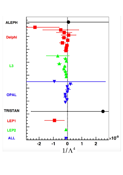
Figure 12: The fit parameter $1/\Lambda^{4}$ measured in units of $1/{\rm GeV}^{4}$ displaied for the data sub-sets, grouped according to their collaborations (ALEPH, Delphi, L3, OPAL), and combinations of collaborations such as TRISTAN (TOPAS and VENUS), LEP 1, and LEP 2. The global combination is labeled by “ALL”.

Table 3: The values of $1/\Lambda^{4}$ in units of GeV^-4 obtained from the fits to data combined in groups of collaborations.

TRISTAN	$(2.49\pm 5.05)\times 10^{-9}$
	$\chi^{2}/dof=50.0/41$
LEP 1	$-(9.20\pm 6.90)\times 10^{-10}$
	$\chi^{2}/dof=32.3/41$
LEP 2	$-(1.10\pm 0.20)\times 10^{-10}$
	$\chi^{2}/dof=267/203$
All Data	$-(1.11\pm 0.20)\times 10^{-10}$
	$\chi^{2}/dof=351/287$

The best fit value of the parameter $1/\Lambda^{4}$ obtained from the $\chi^{2}$ fit is shown in Fig. 13 and listed in Table 4. It has a significance of about five standard deviations, which implies the existence of an excited electron with a mass of $m_{e^{*}}=308\pm 14$ GeV, as interpreted through $\Lambda^{2}_{+}=m^{2}_{e^{*}}/\lambda$, where $\lambda=1.0$.

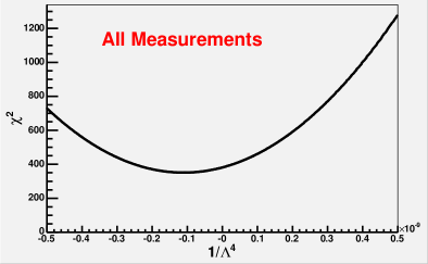
Figure 13: The $\chi^{2}$ as function of $1/\Lambda^{4}\times 10^{-9}$ for all data.

Table 4: Summary of excited electron $\chi^{2}$ tests $(1/\Lambda_{+})_{top}^{4}$ in units ${\rm GeV}^{-4}$.

Heavy electron mass $m_{e^{*}}$
$-(1.11\pm 0.20)\times 10^{-10}$	$\Lambda^{2}_{+}=m^{2}_{e^{*}}/\lambda$	$m_{e^{*}}=308\pm 14$ GeV

4.2 Global $\chi^{2}$ test for a non-pointness of the electron

The $(1-\cos^{2}\theta)$ dependence of the differential cross-section is the same for both the excited electron model (33) and the contact interaction (35). Therefore, the same MINUIT framework can be used to perform the $\chi^{2}$ test by equating $\Lambda=\tilde{\Lambda}=\Lambda_{6}$ in (41).

The difference between (35) and (33) lies only in the presence of the constant $\alpha$, but it does not affect the significance of the fit, as shown in Table 5. The result indicates the existence of a contact interaction with a significance of about five standard deviations and a cutoff scale of $\Lambda_{\rm top}=1253.53\pm 226$ GeV.

Table 5: $\chi^{2}$ tests $(1/\Lambda)_{top}^{4}[GeV^{-4}]$ finite size and heavy electron.

Summary $r_{\rm electron}$ and $m_{e^{*}}$
	Test $r_{electron}$
$-(4.05\pm 0.73)\times 10^{-13}$	$r=(\hbar\times c)/\Lambda$	$r=(1.57\pm 0.07)\times 10^{-17}$ cm
	Test $m_{e^{*}}$
$-(1.11\pm 0.20)\times 10^{-10}$	$\Lambda^{2}_{+}=m^{2}_{e^{*}}/\lambda$	$m_{e^{*}}=308\pm 14$ GeV

Note that the p-value gives a significance result that is very similar to the $\chi^{2}$ test, as demonstrated in detail in the total cross section analysis [77].

5 Indication of a signal in the total cross section

It would be instructive to verify if signal indicating the existence of the excited electron and contact interaction is also present in the total cross-section of the ${\rm e^{+}e^{-}\rightarrow\gamma\gamma(\gamma)}$ reaction.

Studying the sensitivity of the $\chi^{2}$ test to the total experimental cross section $\sigma(\mathrm{tot})$ of the $\rm e^{+}e^{-}\rightarrow\gamma\gamma$ reaction, represented by combined data from different collaborations within the energy range 55 GeV to 207 GeV, is a major challenge. This is due to the fact that different collaborations measured the total cross section $\sigma(\mathrm{tot})$ at different ranges of the angle $\theta$ and with different efficiencies $\varepsilon$ at the same or similar center-of-mass energy. On the other hand, the collaborations compare their measured total cross section $\sigma({\rm tot})$ with a Monte Carlo-simulated [63] QED total cross section $\sigma({\rm QED})$, which is either the same or very similar across all collaborations. Therefore, we choose to use a benchmark L3 detector and normalize the total cross sections measured by other detectors with respect to that of L3, along with the corresponding number of events, as described in [77] in details. This approach enables us to properly combine the center-of-mass energy points where more than one detector has provided measurements of the total cross section. Thereby, one can construct ratios $R({\rm exp})=\sigma({\rm tot,comb})/\sigma({\rm QED})$ by comparing the combined measured total cross section $\sigma({\rm tot,comb})$ to the simulated one $\sigma({\rm QED})$, at each available center-of-mass energy. The unceartanties for $\sigma({\rm tot,comb})$ ($\Delta\sigma({\rm tot,comb})$) and $R({\rm exp})$ ($\Delta R({\rm exp})$) are also calculated. The processed numerical values, initially obtained in [77], are listed in Table 6 and displayed in Fig. 14.

Table 6: Summary of the numerical values for $\sigma({\rm tot,comb})$ R(exp), along with their uncertainties. Refer to the text for details on the processing that was applied.

$\sqrt{s}$ GeV	$\sigma({\rm tot,comb})$ $\Delta\sigma({\rm stat,comb})$ pb	R(exp) $\Delta R({\rm exp})$
55	124.746$\pm$ 13.1736	0.92001 $\pm$ 0.09716
56	150.623 $\pm$ 9.7176	1.15000 $\pm$ 0.07419
56.5	141.633 $\pm$ 22.9310	1.10000 $\pm$ 0.17810
57	135.456 $\pm$ 10.7933	1.07000 $\pm$ 0.08526
57.6	125.311$\pm$ 1.9970	1.01000 $\pm$ 0.01610
91	50.3103 $\pm$ 0.86517	0.98764 $\pm$ 0.01698
133	26.5472 $\pm$ 5.80853	1.09604 $\pm$ 0.23981
162	16.0640 $\pm$ 2.42633	0.98462 $\pm$ 0.14872
172	15.6375 $\pm$ 2.64851	1.08187 $\pm$ 0.18324
183	12.6404 $\pm$ 0.34388	0.99219 $\pm$ 0.02699
189	11.7626 $\pm$ 0.18843	0.98582 $\pm$ 0.01579
192	11.0253 $\pm$ 0.46129	0.95427 $\pm$ 0.03993
196	11.2978 $\pm$ 0.27689	1.02004 $\pm$ 0.02500
200	10.1373 $\pm$ 0.26604	0.95400 $\pm$ 0.02504
202	10.1199 $\pm$ 0.37855	0.97204 $\pm$ 0.03636
205	9.98539 $\pm$ 0.32275	0.98865 $\pm$ 0.03196
207	9.66178 $\pm$ 0.23860	0.97594 $\pm$ 0.02410

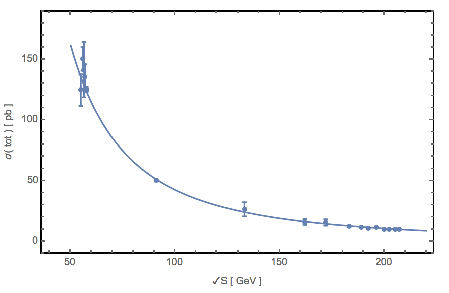
Figure 14: The $\sigma$(tot) of the $\rm e^{+}e^{-}\rightarrow\gamma\gamma(\gamma)$ reaction of all detectors as function of centre-of-mass energy $\sqrt{s}$. The data (points) are compared to QED prediction (solid line).

No significant disagreement between the combined measured total cross section ($\sigma({\rm tot,comb})$) of the $\rm e^{+}e^{-}\rightarrow\gamma\gamma$ reaction in the center-of-mass energy range 55.0 GeV$\leq$ $\sqrt{s}$ $\leq$207 GeV and the predicted value $\sigma({\rm QED})$ is observed in Fig. 14. The decrease in uncertainties is observed at higher center-of-mass energy band (so called LEP energies) due to the contribution of multiple detectors to each $\sqrt{s}$ point. To show the potential impact of the parameters inferred at five standard deviations significance from the $\chi^{2}$ test of the differential cross section, we plot in Fig. 15 the ratio $R({\rm exp})$ along with ratio $R({\Lambda_{6}})=\sigma(QED)_{\rm tot}^{\rm L3}/\sigma({\rm QED}+\Lambda_{\rm top})_{\rm tot}^{\rm L3}$, where $\sigma(QED)_{\rm tot}^{\rm L3}$ and $\sigma({\rm QED}+\Lambda_{\rm top})_{\rm tot}^{\rm L3}$ are the pure QED and the excited electron (contact interaction) modified at $\Lambda_{\rm top}=1253.53$ GeV total cross sections normalized with respect to L3 detector. For $R({\Lambda_{6}})$ we adopt an analytical approximation

$$R(\Lambda{{}_{6}})=C_{4}+C_{1}\cdot(-Tanh[C_{3}\sqrt{s}+C_{2}])\ ,$$ (42)

where the constants $C_{1}=0.0732964$, $C_{2}=-3.06655$, $C_{3}=0.0127994$ and $C_{4}=0.928311$ are obtained from the fit of the Monte Carlo generated numerical results on $R({\Lambda_{6}})$. The experimental data show (Fig. 15) a deviation from the QED prediction above $\sqrt{s}=180$ GeV.

In summary, Figure 15 indicates a deviation between the total cross section of the measured data and the QED prediction, in contrast to the differential cross section test shown in Figures 6 to 11. The data tend to lie below the horizontal line in the energy range $\sqrt{s}\gtrsim 180$ GeV, with $R(\Lambda_{6})$ being approximately 4.0% lower than the QED predicted values.

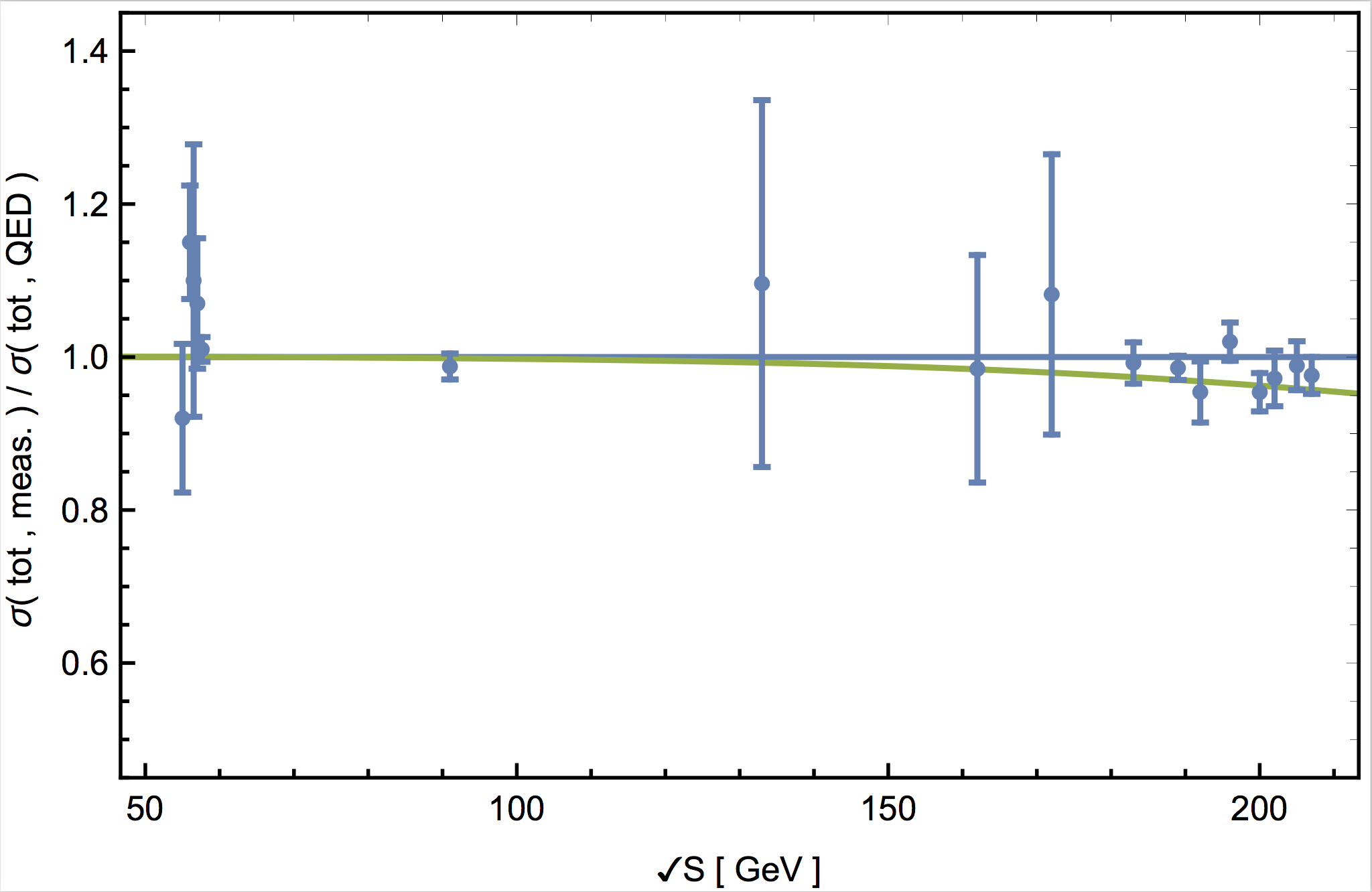
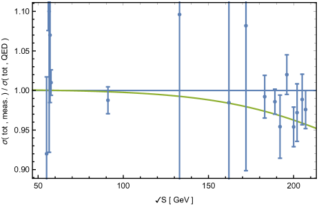
Figure 15: The ratio $R({\rm exp})$ along with ratio $R({\Lambda_{6}})=\sigma(QED)_{\rm tot}^{\rm L3}/\sigma({\rm QED}+\Lambda_{\rm top})_{\rm tot}^{\rm L3}$, where $\sigma(QED)_{\rm tot}^{\rm L3}$ and $\sigma({\rm QED}+\Lambda_{\rm top})_{\rm tot}^{\rm L3}$ are the pure QED and the excited electron (contact interaction) modified at $\Lambda_{\rm top}=1253.53$ GeV total cross sections normalized with respect to L3 detector. Right panel represents a zoomed version of the plot.

6 Systematic uncertainties

Various sources of systematic uncertainties contribute to the measurement, including uncertainties from the luminosity evaluation, selection efficiency, background estimation, choice of QED-$\alpha^{3}$ theoretical cross section, fit procedure, fit parameter, and the choice of scattering angle in $|\cos\theta|$ for comparison between data and theory. The maximum estimated uncertainties from luminosity, selection efficiency, and background evaluations contribute approximately $\delta\Lambda/\Lambda=0.01$ to the total systematic uncertainty in the estimated fit parameter. The choice of theoretical QED cross section was validated using about 2 kilo $\rm e^{+}e^{-}\rightarrow\gamma\gamma(\gamma)$ events generated and processed with the geometry and selection cuts of the L3 detector [79, 63]. For scattering angles close to 90^∘ where $|\cos(\theta)|_{\mathrm{experiment}}\sim 0.05$, the systematic uncertainty contribution $(\delta\Lambda/\Lambda)_{\delta|\cos\theta|}$ is approximately 0.01. The combined effect of these two systematic uncertainties yields the uncertainty of $\delta\Lambda/\Lambda\approx 0.015$. In a small sample of $\rm e^{+}e^{-}\rightarrow\gamma\gamma(\gamma)$ events, fit values were compared using $\chi^{2}$, maximum likelihood, Smirnov-Cramer von Mises, and Kolmogorov tests with and without binning [80]. An additional uncertainty of $\delta\Lambda/\Lambda=0.005$ was inferred from the fit procedure variation study. In summary, while multiple sources of systematic uncertainties have been identified, they are all smaller than the statistical uncertainty of the experimental data.

A slight deviation in $R({\rm exp})$ from the $\sigma({\rm QED})_{\rm tot}$ cross section appears in Table 6 and Figure 15 above $\sqrt{s}=91.2$ GeV. The systematic uncertainty for the measured total cross section above $\sqrt{s}>91.2$ GeV ranges from 0.10 pb to 0.13 pb for L3 (see Table 3 in [56]), 0.09 pb to 0.14 pb for DELPHI (see Table 4 in [54]), and 0.05 pb to 0.08 pb for OPAL (see Table 7 in [56]). The systematic uncertainty for the total QED cross section of each detector is taken at the level $\Delta\sigma(QED){sys}=0.1$ pb [56] for every detector above $\sqrt{s}=$ 91.2 GeV. Thus it is quite unlikely that the deviation of $R({\rm exp})$ from $R({\rm QED})$ could originate from systematic uncertainties. For further information, refer to [77].

7 Concluding remarks

The VENUS, TOPAS, OPAL, DELPHI, ALEPH, and L3 collaborations measured the differential cross section of the $\rm e^{+}e^{-}\rightarrow\gamma\gamma(\gamma)$ reaction to test QED. Except for ALEPH, all collaborations observed a negative deviation from the QED, although with low significance. The total cross-section test of LEP2 and the comparison with measurements in Figure 15 support these negative trends. We performed a thorough $\chi^{2}$ analysis using all available data to search for evidence of an excited electron $e^{*}$ and a finite annihilation length, using a direct contact term approach. By conducting a global analysis of the combined data-sets, it was possible for the first time to establish a significance of approximately 5$\times\sigma$ on the mass of an excited electron, which is $m_{e^{*}}=308\pm 56$ GeV. A similar 5$\times\sigma$ significance effect was detected for a charge distribution radius of the electron, $r=(1.57\pm 0.07)\times 10^{-17}$ cm. Therefore, by combining the full statistical power of all available LEP and non-LEP high efficiency experiments on measurements of the cross section of the reaction of annihilation in $e^{+}e^{-}$ collisions, allowed us to identify the signal of existence of excited electron and contact interaction of at a high level of significance. Previous analyses had restricted themselves to data collected only by LEP detectors and not at all LEP energies. Therefore, combining the full statistical power of all available LEP and non-LEP high efficiency experiments on measurements of the cross section of the reaction of annihilation in $e^{+}e^{-}$ collisions, we were able to recognize the signal of the existence of an excited electron and contact interaction at a high level of significance. Previous analyses had only combined data collected by LEP detectors and at a limited range of LEP energies.

Extensive measurements and analyses were conducted to search for quark and lepton compositeness in contact interaction [85], specifically in the Bhabha channel as shown in Figure 1. A hint of axial-vector contact interaction was observed in the data on $e^{+}e^{-}\rightarrow e^{+}e^{-}(\gamma)$ scattering from ALEPH, DELPHI, L3, and OPAL at centre-of-mass energies ranging from 192 to 208 GeV. The detection was made at $\Lambda=10.3^{+2.8}_{-1.6}$ TeV [86].

At the Z⁰ pole, the $\rm e^{+}e^{-}\rightarrow\gamma\gamma(\gamma)$ reaction exhibits a suppression of the s-channel, resulting in $R(\Lambda_{6})=0.999$, demonstrating perfect agreement. Alternatively, in a Bhabha-like reaction ($e^{+}e^{-}\rightarrow e^{+}e^{-}(\gamma)$), a different QED test is used to search for $m_{e^{*}}$, utilizing pair-production in the s-channel through $\gamma$ and Z boson exchange, similar to Bhabha scattering in Fig. 1. The mass values or limits for an excited electron depend on the test reaction used for its study and the theoretical interpretation of $\Lambda$ values. For example, in the case of $\rm e^{+}e^{-}\rightarrow\gamma\gamma(\gamma)$ reaction, these values can be obtained from the Lagrangian (30) or equation (4) in [56]. The L3-collaboration set lower limits on 95% CL for pair-production of neutral heave leptons, from $m_{L}^{*}>102.7$ GeV to $m_{L}^{*}>80.5$ GeV, depending on the model (Dirac or Majorana). They also set lower limits at 95% CL for pair-produced charged heavy leptons from $m_{L}^{*}>102.6$ GeV to $m_{L}^{*}>100.8$ GeV. Similarly, the OPAL-collaboration set lower limits on 95% CL for long-lived charged heavy leptons and charginos by $(m_{L^{*}},m_{chargino})>102.0$ GeV, as well as lower limits on neutral $L^{0}$ and charged $L^{\pm}$ heavy leptons [83]. The HERA H1 collaboration searched for heavy leptons and obtained best-fit limits for an $e^{*}$ production in the HERA mass range in the $\gamma$ final state, with a composite scale parameter $\Lambda$ excluding values below approximately 300 GeV.

The CMS collaboration is searching for long-lived charged particles in pp collisions [87] using a modified Drell-Yan production process. This involves the annihilation of a quark and an antiquark from two different hadrons, producing a pair of leptons through the exchange of a virtual photon or $Z^{0}$ in the s-channel. The study excluded Drell-Yan signals with $|Q|=1e$ below masses of 574 GeV/$c^{2}$.

The latest experimental data from hadronic machines [90, 91, 92, 93] do not provide evidence for excited leptons, setting an exclusion limit on the excited electron mass is $m_{e^{*}}=3$ TeV for the reaction of single production like $ep\rightarrow e^{*}X\rightarrow\gamma X$, which is different from double $e^{*}$ production investigated in $e^{+}e^{-}$ scattering reaction. The future colliders with higher centre-of mass enrgy and luminosity will continue the search for the excited leptons. The production of two photons at large angles in $e^{+}e^{-}$ annihilation has been suggested as a way to measure the luminosity of future circular and linear colliders. These colliders, including FCC-ee [94], CEPC [95], ILC [96], and CLIC [97], will have polarized beams and can be used to test the accuracy of the Standard Model and search for signals of new physics.

The exchange of the excited electron does not produce non-zero polarization effects in the case of only one polarized beam [98], at least in the lowest order of perturbation theory. This is because the reaction that produces the excited electron conserves space parity, which can be inferred from the expression for the Lagrangian (30). From the other side, contact interaction affects the polarization observables in reaction $\rm e^{+}e^{-}\rightarrow\gamma\gamma(\gamma)$ when the initial particles are polarized. In the general case, the contact interaction violates space parity [98]. Therefore, non-zero observables arise only when one of the beams is polarized. The pure QED mechanism of this reaction, without taking radiative corrections into account, does not produce such polarization effects. However, electroweak corrections (at the one-loop level, as shown in [99]) can introduce an additional term to the amplitude of this process that violates parity and, therefore, can lead to non-zero polarization observables. The future colliders that were mentioned earlier, which employ polarized beams, offer a promising opportunity for experimental investigation into the polarization effects of contact interactions.

Based on the results of our analysis, a possible manifestation of the non-point nature of the electron can be speculated using a model [35, 88] that proposes an electromagnetic spinning soliton for the electron with a de Sitter vacuum disk generating an electric and magnetic field. This opens up the possibility of constructing a wave function of the electric field, which, when connected with the model [88], results in a Lorenz Contracted radius that agrees with the experiment at approximately $r_{e}\sim 1.57\times 10^{-17}$ cm [88, 89]. The numerical coincidence between [35], [88, 89] and the experiment may imply a manifestation of the non-point nature of the electron within the frameworks of [35, 88, 89].

We can speculate that depending on the experimental tests, the electron may exhibit two types of extended interiors. Indeed, in the $\rm e^{+}e^{-}\rightarrow\gamma\gamma(\gamma)$ reaction, only the QED long-range interaction is tested, while the weak interaction via $Z^{0}$ is suppressed by angular momentum conservation. As a result, $\Lambda_{top}$ of $1253.53\pm 226$ GeV obtained in our analysis is interpretted in terms of size of electron, which amounts $r_{e}\sim 1.57\times 10^{-17}$ cm. On the other hand, in the Bhabha reaction $e^{+}e^{-}\rightarrow e^{+}e^{-}(\gamma)$, the short-range weak and QED interactions are involved. Due to the much larger differential cross section in the Bhabha channel compared to that in the pure QED channel, this channel dominates. Moreover, the inclusion of the $Z^{0}$ contribution in the reaction results in a significantly higher $\Lambda$ of $10.3^{+2.8}_{-1.6}$ TeV compared to the $\rm e^{+}e^{-}\rightarrow\gamma\gamma(\gamma)$ reaction, which in turn leads to an eight-fold reduction in extension if interpreted in terms of a radius. Based on the observed data and analysis, it is tantalizing to suggest that the electron may possess not just one, but two distinct interiors, an outer and inner core. With these intriguing findings, we can tantalizingly speculate that the humble electron is not just a simple point particle, but rather a complex entity with both an outer and inner core. Could it be that two attributes are combined in this particle, as some theories have suggestedn [35]? The possibilities are truly fascinating and open up new avenues for further exploration and discovery in the field of particle physics.

References

-
[1]
“Premier mémoire sur l’électricité et le magnétisme,” Histoire de l’Académie Royale des Sciences, pp. 569 - 577.
“Second mémoire sur l’électricité et le magnétisme,” Histoire de l’Académie Royale des Sciences, pages 578 - 611.
-
[2]
Whittaker, E. T. (1910). A History of the Theories of Aether and Electricity. Dover Publications. ISBN 978-0-486-26126-3.
Oersted, John Christian (1820). “Experiments on the effect of a current of electricity on the magnetic needle”. Annals of Philosophy 16 . 273-276. -
[3]
Christine Blondel: A.-M. Ampere et la creation de l’electrodynamique 1820-1827, Paris, Bibliotheque Nationale 1982.
Blundel, Stephen J. ( 2012 ) Magnetism: A Very Short Introduction .OUP Oxford p. 31 ISPN 9780191633720
Tricker, R.A.R. ( 1965 ) Early electrodynamics Oxford Pergamon p. 23. - [4] A joint Biot-Savart paper Note sur le magnètisme de la pile de Volta was published in the Annales de chemie et de physique in 1820.
-
[5]
Martin, Andre (1986), “Cathode Ray Tubes for Industrial and Military Applications”, in Hawkes, Peter (ed.),
Advances in Electronics and Electron Physics,Volume 67, Academic Press, p. 183, ISBN 9780080577333,
“Evidence for the existence of cathode-rays” was first found by Plücker and Hittorf …
Joseph F. Keithley The story of electrical and magnetic measurements: from 500 B.C. to the 1940s John Wiley and Sons, 1999 ISBN 0-7803-1193-0, page 205 -
[6]
E. Goldstein (May 4, 1876) “Vorläufige Mittheilungen über elektrische Entladungen in verdünnten Gasen”
(Preliminary communications on electric discharges in rarefied gases), Monatsberichte der Königlich Preussischen
Akademie der Wissenschaften zu Berlin (Monthly Reports of the Royal Prussian Academy of Science in Berlin), 279-295.
From page 286: “13. Das durch die Kathodenstrahlen in der Wand hervorgerufene Phosphorescenzlicht ist höchst
selten von gleichförmiger Intensität auf der von ihm bedeckten Fläche, und zeigt oft sehr barocke Muster.” (13.
The phosphorescent light that’s produced in the wall by the cathode rays is very rarely of uniform intensity on the surface that
it covers, and [it] often shows very baroque patterns.)
Joseph F. Keithley The story of electrical and magnetic measurements: from 500 B.C. to the 1940s John Wiley and Sons, 1999 ISBN 0-7803-1193-0, page 205 - [7] “Joseph John Thomson”. Science History Institute. June 2016. Retrieved 20 March 2018.
-
[8]
Edward Arthur Davis, Isobel J. Falconer: J. J. Thompson and the Discovery of the Electron.
Taylor - Francis, London 1997, ISBN 0-7484-0696-4.
CATHODE Rays ( Charge - mass - ratio ) Philosophical Magazine, 44, 293-316 (1897). -
[9]
Millikan Experiment. Nobel Prize in Physics in 1923. “The Nobel Prize in Physics 1923”. NobelPrize.org. Retrieved 2019-07-31.
Elementary charge ELECTRON 2019. “2018 CODATA Value: elementary charge”. The NIST Reference on Constants, Units, and Uncertainty. NIST. 20 May 2019.
Elementary mass ELECTRON 2019. Mohr, P.J.; Taylor, B.N.; Newell, D.B. “2018 CODATA recommended values”. National Institute of Standards and Technology. Gaithersburg, MD: U.S. Department of Commerce. Archived from the original on 2018-01-22. Retrieved 2019-12-03. “This database was developed by J. Baker, M. Douma, and S. Kotochigova.” - [10] Abraham, “M. Prinzipien der Dynamik des Elektrons” ,Ann. Phys. 1903 10. 105 - 179.
- [11] Lorentz, H.A. Electromagnetic phenomena in a system moving with any velocity smaller than that of light. Proc. R. Neth. Acad. Arts Sci. 1904, 6, 809 - 831.
- [12] Lorentz, H.A. Theory of Electrons, 2nd ed.; Dover: New York, NY, USA, 1952.
- [13] Dirac, P.A.M. Classical theory of radiating electrons. Proc. R. Soc. Lond. 1938, A167, 148 - 169.
-
[14]
Compton, Arthur H. (August 1921). “The Magnetic Electron”. Journal of the Franklin Institute. 192 (2):
145?155. doi:10.1016/S0016-0032(21)90917-7.
Charles P. Enz, Heisenberg’s applications of quantum mechanics (1926-33) or the settling of the new land, Department de Physique Thorique Universit de Genve, 1211 Genve 4, Switzerland (10. I. 1983). - [15] Gerlach, W.; Stern, O. (1922). “Der experimentelle Nachweis der Richtungsquantelung im Magnetfeld”. Zeitschrift für Physik. 9 (1): 349?352. Bibcode:1922ZPhy….9..349G. doi:10.1007/BF01326983. S2CID 186228677.
- [16] Pauli, W. (1925). “ Über den Zusammenhang des Abschlusses der Elektronengruppen im Atom mit der Komplexstruktur der Spektren”. Zeitschrift für Physik. 31 (1): 765?783. Bibcode:1925ZPhy…31..765P. doi:10.1007/BF02980631. S2CID 122941900.
-
[17]
P.W. SCHMOR, “ A Review of Polarized Ion Sources - CERN ”.
https://accelconf.web.cern.ch MPE MPE01.
W. Haeberli, “ Sources of Polarized Ions ”. Annual Review of Nuclear Science. Vol. 17:373 - 426 (Volume publication date December 1967) https://doi.org/10.1146/annurev.ns.17.120167.002105. -
[18]
W. Arnold, J. Ulbricht, H. Berg, P. Keiner, H.H. Krause, R. Schmidt and G. Clausnitzer
“ The Giessen polarization facility 2, 1.2 MeV tandem accelerator”.
Nucl. Instr. and Meth. 143 (1977) 457.
H.H. Krause, R. Stock, W. Arnold, H. Berg, E. Huttel, J. Ulbricht and G. Clausnitzer, “ The Giesssen polarization facility 3. Multi-detector analyzing system ”. Nucl. Instr. and Meth. 143 (1977) 467. -
[19]
According to William Barletta, director of USPAS, the US Particle Accelerator School,
per Toni Feder, in Physics Today February 2010, “Accelerator school travels university circuit”, p. 20
Minehara, Eisuke; Abe, Shinichi; Yoshida, Tadashi; Sato, Yutaka; Kanda, Mamoru; Kobayashi, Chiaki; Hanashima, Susumu (1984). “On the production of the KrF- and XeF- Ion beams for the tandem electrostatic accelerators”. Nuclear Instruments and Methods in Physics Research Section B. 5 (2): 217. Bibcode:1984NIMPB…5..217M. doi:10.1016/0168-583X(84)90513-5. -
[20]
Szczerba, Dominik,“ Development of a polarized atomic beam source and measurement of spin correlation parameters ”.
Diss., Naturwissenschaften ETH Zürich, Nr. 14261, 2001. https://doi.org/10.3929/ethz-a-004176559.
A. Nass, M. Stancari and E. Steffens, “ Studies on Beam Formation in an Atomic Beam Source”. August 2009 AIP Conference Proceedings 1149(1):863, DOI:10.1063/1.3215780 - [21] G. Aruldhas (2009). “5.15 Lamb Shift”. Quantum Mechanics (2nd ed.). Prentice-Hall of India Pvt. Ltd. p. 404. ISBN 978-81-203-3635-3.
-
[22]
Thomas B. Clegg, “ Lamb - shift polarized ion sources - after 15 years ”, AIP Conference Proceedings 80, 21 (1982);
https://doi.org/10.1063/1.33417.
W. Arnold, H. Berg, H.H. Krause, J. Ulbricht and G. Clausnitzer, “ The Giessen poarization facility 1. Lamb shift source ” Nucl. Instr. and Meth. 143 (1977) 441.
J. Ulbricht, W. Arnold, H. Berg, E. Huttel, H.H. Krause and G. Clausnitzer, “ The polarised proton capture reaction 7Li()8Be in the energy range from 380 to 960 keV ”. Nucl. Phys. A287 (1977) 2 -
[23]
W. Haeberli, “ Sources of Polarized Ions ”. Annual Review of Nuclear Science.
Vol. 17:373 - 426 (Volume publication date December 1967)
https://doi.org/10.1146/annurev.ns.17.120167.002105.
Raymond, Richard Stephen, “ An intense source of negative polarized hydrogen ions ”. Thesis–University of Wisconsin–Madison, 1979. Bibliography: leaves 123-126. - [24] Schrödinger, E. “ Über die kräftefreie Bewegung in der relativistischen Quantenmechanik ”. Sitzunber. Preuss. Akad. Wiss. Phys. Math. Kl. 1930, 24, 418 - 428.
-
[25]
Weyssenhoff, J.; Raabe, “ A. Relativistic dynamics of spin fluids and spin-particles”. Acta Phys. Pol. 1947, 9, 7?18.
Pryce, M.H.L. “ The mass-centre in the restricted theory of relativity and its connexion with the quantum theory of elementary particles”. Proc. R. Soc. 1948, A195, 62?81.
Fleming, C.N. “ Covariant position operators, spin, and locality ”. Phys. Rev. 1965, B 137, 188 - 197. [CrossRef]
Riewe, F. “ Generalized mechanics of a spinning particle ”. Lett. Nuovo Cim. 1971, 1, 807 - 808. [CrossRef]
Barut, A.O.; Zanghí, “ N. Classical model of the Dirac electron ”. Phys. Rev. Lett. 1984, 52, 2009 - 2012. [CrossRef] - [26] M. Srednicki, “Quantum field theory,” Cambridge University Press, 2007, ISBN 978-0-521-86449-7, 978-0-511-26720-8
- [27] M. E. Peskin and D. V. Schroeder, “An Introduction to quantum field theory,” Addison-Wesley, 1995, ISBN 978-0-201-50397-5
- [28] M. D. Schwartz, “Quantum Field Theory and the Standard Model,” Cambridge University Press, 2014, ISBN 978-1-107-03473-0, 978-1-107-03473-0
- [29] M. Thomson, “Modern particle physics,” Cambridge University Press, 2013, ISBN 978-1-107-03426-6 doi:10.1017/CBO9781139525367
- [30] C. Itzykson and J. B. Zuber, “Quantum Field Theory,” McGraw-Hill, 1980, ISBN 978-0-486-44568-7
-
[31]
Frenkel, J. “ Die Elektrodynamik des rotierenden Elektrons. ”.Z. Phys. 1926, 37, 243 - 262. [CrossRef]
Mathisson, M. “ Neue Mechanik materieller Systeme ”. Acta Phys. Pol. 1937, 6, 163 - 200.
Kramers, L.H. “ Quantentheorie des Electron und der Strahlung ”. Akademische Verlagsgesellschaft: Leipzig, Germany, 1938.
Hönl, H.; Papapetrou, A. “ Über die innere Bewegung des Elektrons ”. Z. Phys. 1939, 112, 512 - 540. [CrossRef]
Bhabha, H.J.; Corben, A.C. “ General classical theory of spinning particles in a Maxwell field ”. Proc. R. Soc. 1941, A178, 273.
Bargman, V.; Michel, L.; Telegdi, “ V.L. Precession of the polarization of particles moving in a homogeneous electromagnetic field ”. Phys. Rev. Lett. 1959, 2, 435 - 436. [CrossRef]
Nash, P.L. “ A Lagrangian theory of the classical spinning electron ”. J. Math. Phys. 1984, 25, 2104 - 2108. [CrossRef]
Plyushchay, M.S. “ Relativistic massive particle with higher curvatures as a model for the description of bosons and fermions ”. Phys. Lett. 1990, B235, 47?51. [CrossRef]
Yee, K.; Bander, “ M. Equations of motion for spinning particles in external electromagnetic and gravitational fields ”. Phys. Rev. 1993, D48, 2797 - 2799. [CrossRef] [PubMed]
Bolte, J.; Keppeler, S. “ Semiclassical form factor for chaotic systems with spin ”. J. Phys. 1999, 32, 8863 - 8880. [CrossRef] -
[32]
Nesterenko, V.V. “ Singular Lagrangians with higher derivatives ”. J. Phys. A Math. Gen. 1989, 22, 1673 - 1687. [CrossRef]
Rylov, Y.A. “ Spin and wave function as attributes of ideal fluid ”. J. Math. Phys. 1999, 40, 256 - 278. [CrossRef] -
[33]
Rivas, M. Kinematical “ Theory of Spinning Particles ”;
Kluwer: Dordrecht, The Netherlands, 2001.
Rivas, M. “ The dynamical equation of the spinning electron ”. J. Phys. A Math. Gen. 2003, 36, 4703 - 4716. [CrossRef] - [34] Newman, E.T.; Cough, E.; Chinnapared, K.; Exton, A.; Prakash, A.; Torrence, R. “ Metric of a Rotating, Charged Mass ”. J. Math. Phys. 1965, 6, 918?919. [CrossRef]
- [35] Irina. Dymnikova, “ Image of the Electron Suggested by Nonlinear Electrodynamics Coupled to Gravity ” Particles 2021, 4(2), 129-145; https://doi.org/10.3390/particles4020013.
- [36] H. Terazawa, M. Yasue, K. Akama and M. Hayashi, “Observable Effects of the Possible Substructure of Leptons and Quarks,” Phys. Lett. B 112 (1982), 387-392 doi:10.1016/0370-2693(82)91075-9
- [37] F. M. Renard, “Excited Quarks and New Hadronic States,” Nuovo Cim. A 77 (1983), 1
- [38] A. De Rujula, L. Maiani and R. Petronzio, “Search for Excited Quarks,” Phys. Lett. B 140 (1984), 253-258 doi:10.1016/0370-2693(84)90930-4
- [39] E. Eichten, K. D. Lane and M. E. Peskin, “New Tests for Quark and Lepton Substructure,” Phys. Rev. Lett. 50 (1983), 811-814 doi:10.1103/PhysRevLett.50.811
- [40] H. Terazawa, K. Akama and Y. Chikashige, “Unified Model of the Nambu-Jona-Lasinio Type for All Elementary Particle Forces,” Phys. Rev. D 15 (1977), 480 doi:10.1103/PhysRevD.15.480
- [41] Y. Ne’eman, “PRIMITIVE PARTICLE MODEL,” Phys. Lett. B 82 (1979), 69 doi:10.1016/0370-2693(79)90427-1
- [42] U. Baur, M. Spira and P. M. Zerwas, “Excited Quark and Lepton Production at Hadron Colliders,” Phys. Rev. D 42 (1990), 815-824 doi:10.1103/PhysRevD.42.815
- [43] F. E. Low, “Heavy electrons and muons,” Phys. Rev. Lett. 14 (1965), 238-239 doi:10.1103/PhysRevLett.14.238
- [44] F. Boudjema, “SUBSTRUCTURE EFFECTS AT LEP100,” Int. J. Mod. Phys. A 6 (1991), 1-20 doi:10.1142/S0217751X91000022
- [45] H. Harari, “COLORED LEPTONS,” Phys. Lett. B 156 (1985), 250-254 doi:10.1016/0370-2693(85)91518-7
-
[46]
De Sitter, W. (1917), “ On the relativity of inertia: Remarks concerning Einstein’s latest hypothesis” (PDF),
Proc. Kon. Ned. Acad. Wet., 19: 1217- 1225
De Sitter, W. (1917), “ On the curvature of space” (PDF), Proc. Kon. Ned. Acad. Wet., 20: 229?243 - [47] Dymnikova, I. “ De Sitter-Schwarzschild black hole: Its particle like core and thermodynamical properties ”. Int. J. Mod. Phys. 1996, D5, 529 - 540. [CrossRef]
-
[48]
John Bardeen; Leon Cooper; J. R. Schriffer (December 1, 1957). “ Theory of Superconductivity ”. Physical Review. Vol. 108. p. 1175.
John Daintith (2009). “ The Facts on File Dictionary of Physics (4th ed.) ”. Infobase Publishing. p. 238. ISBN 978-1-4381-0949-7.
John C. Gallop (1990). “ SQUIDS, the Josephson Effects and Superconducting Electronics. ” CRC Press. pp. 1, 20. ISBN 978-0-7503-0051-3
Durrant, Alan (2000). “ Quantum Physics of Matter ”. CRC Press. pp. 102?103. ISBN 978-0-7503-0721-5. - [49] Pospelov, M.; Ritz, A. (2005). “Electric dipole moments as probes of new physics”. Annals of Physics. 318 (1): 119 - 169. arXiv:hep-ph/0504231.
- [50] Abe, K.; et al.; VENUS Collaboration. Measurements of the differential cross sections of and at = 55, 56, 56.5 and 57 GeV. Z. Phys. C 1989, 45,175.
- [51] Akrawy, M.Z.; et al.; OPAL Collaboration. Measurements of the cross sections of the reaction and at LEP. Phys. Lett. B 1991, 257,531.
- [52] Shimozawa, K.; et al.; TOPAS Collaboration. Studies of and reaction. Phys. Lett. B 1992, 284, 144.
- [53] Decamp, D.; et al.; ALEPH Collaboration. Search for new particles in Z decays using the ALEPH detector. Phys. Rept. 1992, 216, 253.
-
[54]
Abreu, P.; et al.; DELPHI Collaboration. Measurement of the cross section at LEP energies.
Phys. Lett. B 1994, 327, 386.
Abreu, P.; et al.; DELPHI Collaboration. Measurement of the cross section at LEP energies. Phys. Lett. B 1998, 433, 429.
Abreu, P.; et al.; DELPHI Collaboration. Determination of the cross-section at centre-of-mass energies ranging from 189 GeV to 202 GeV.
Phys. Lett. B 2000, 491, 67. - [55] Acciarri, M.; et al.; L3 Collaboration. Test of QED at LEP energies using and . Phys. Lett. B 1995, 353,136.
- [56] Achard, P.; et al.; L3 Collaboration. Study of multiphoton final states and tests of QED in collisions at up to 209 GeV. Phys. Lett. B 2002, 531,28.
- [57] The ALEPH Collaboration; The DELPHI Collaboration; The L3 Collaboration; The OPAL Collaboration; The LEP Electroweak Working Group. Electroweak Measurements in Electron-Positron Collisions at W-Boson-Pair Energies at LEP. Report CERN-PH-EP/2013-022, arXiv 2013, arXiv:1302.3415v4 [hep-ex]; CERN: Geneva, Switzerland, 2013.
-
[58]
Irina Dymnikova, Alexander Sakharov and Jürgen Ulbricht. “Appearance of a Minimal Length in Annihilation”.
Hindawi Publishing Corporation Advances in High Energy Physics Volume 2014, Article ID 707812, 9 pages
http://dx.doi.org/10.1155/2014/707812
Bajo, A.; et al. QED test at LEP200 energies in the reaction . AIP Conference Proceedings 2001, 564, 255.
Dymnikova, I.G.; Hasan, A.; Ulbricht, J.; J. Zhao, J. “ Limits on the Sizes of Fundamental Particles and Gravitational Mass of the Higgs Particle ”. Gravitation and Cosmology 2001, 7, 122.
- [59] Abbiendi, G.; et al.; OPAL Collaboration. Multi-photon production in collisions at = 181-209 GeV. Eur. Phys. J. C 2003, 26, 331.
-
[60]
Xe, Jingbo. Physics with final states at the energy scale using Electron - Positron collision.
M. S. thesis, Chinese University of Science and Technology 1992, private communication.
USTC Hefei, Anhui 230 029, China 1992.
Wu, Jian. Tests of Quantum Electrodynamics at the Scale. M. S. thesis, Chinese University of Science and Technology 1997, No. JX1612-477. USTC Hefei, Anhui 230 029, China 1997.
Zhao, Jiawei. Tests of QED using reactions at LEP200 and study of inclusive semileptonic D meson decays at BES. M. S. thesis, Chinese University of Science and Technology 2001, No. JX1612-647. USTC Hefei, Anhui 230 029, China 2001. - [61] CERN yellow book “ HIGGS SEARCH AND NEW PHYSICS” 1989, 2 ,89; CERN: Geneva, Switzerland, 1989.
-
[62]
Adriani, O.; et al.; L3 Collaboration. A test of quantum electrodynamics in the reaction .
Phys. Lett. B 1992, 288, 404.
Acciarri, M.; et al.; L3 Collaboration. Observation of multiple hard photon final states at = 130 -140 GeV at LEP. Phys. Lett. B 1996, 384, 323.
Acciarri, M.; et al.; L3 Collaboration. Hard-photon production at = 161 and 172 GeV at LEP. Phys. Lett. B 1997, 413, 159.
Acciarri, M.; et al.; L3 Collaboration. Hard-photon production and tests of QED at LEP. Phys. Lett. B 2000, 475, 1987. -
[63]
Berends, F.A. Kleiss, R. DISTRIBUTIONS FOR ELECTRON-POSITRON ANNIHILATION INTO
TWO AND THREE PHOTONS. Nucl. Phys. B 1981, 186, 22.
CALKUL Collaboration, F.A. Berends et al., Nucl. Phys. B 239 (1984) 395.
F.A. BERENDS, R. GASTMANS, HARD PHOTON CORRECTIONS FOR
Nuclear Physics B61 (1973) 414-428.
BabaYaga@NLO; https://inspirehep.net/literature/1740483 ; http://www.pv.infn.it/hepcomplex/babayaga.html; EPJ Web of Conferences 218, 07004 (2019) PhiPsi 2017. - [64] Mandl, F.; Skyrme,T. H. R. The theory of the double Compton effect. Proceedings of the Royal Society A 1952, 215, 497.
- [65] P. Mery, M. Perrottet and F. M. Renard, “Anomalous Effects in Annihilation Into Boson Pairs. 2. , , ,” Z. Phys. C 38 (1988), 579 doi:10.1007/BF01624363
-
[66]
King, S.F.; Sharpe S.R. EXOTIC CERN EVENTS FROM EXOTIC COLOR STATES.
Nucl. Phys. B 1985, 253, 1.
Leung, C.N.; Love, S.T.; Rao, S. Low-Energy Manifestations of a New Interactions Scale: Operator Analysis. Z. Phys. C 1986, 31, 433.
Drell, S.D.; Parke, S.J. Constraints on Radiative Decays. Phys. Rev. Lett. 1984, 53, 1993.
Dicus, D.A.; Tata, Xerxes. Anomalous photon interactions. Phys. Lett. B 1985, 155, 103.
Dicus, D.A. New interactions and neutrino counting. Phys. Rev. D 1985, 31, 2999. - [67] Eboli, O.J.P.; Natale, A.A.; Novaes, S.F. Bounds on effective interactions from the reaction at LEP. Phys. Lett. B 1991, 271, 274.
- [68] Litke, A.M. Experiments with electron-positron colliding beams. M. S. thesis, Havard University 1970, private communication. Harvard College, Cambridge, Massachusetts, US 1970.
- [69] A. Kempf, G. Mangano, and R. B. Mann, “ Hilbert space representation of the minimal length uncertainty relation,” Physical Review D, vol. 52, no. 2, 1108 - 1118 (1995)
- [70] A. Kempf and G. Mangano, “ Minimal length uncertainty relation and ultraviolet regularization,” Physical Review D, vol. 55, no. 12 7909 - 7920 (1997)
- [71] A. Kempf, “ Mode generating mechanism in inpation with a cutoff, ” Physical Review D, vol. 63, no. 8, Article ID 083514 5 pages, (2001)
-
[72]
Khan Academy, “ Light: Electromagnetic waves,
the electromagnetic spectrum photons ”,
https://www.khanacademy.org/science/physics
/light-waves/introduction-to-light-waves
/a/light-and-the-electromagnetic-spectrum - [73] S. Hossenfelder, “ Minimal length scale scenarios for quantum gravity, ” Living Reviews in Relativity, vol. 16 2 (2013)
- [74] Pasquale Bosso, Saurya Das, Vasil Todorinov, “Quantum field theory with the generalized uncertainty principle II: Quantum Electrodynamics”, Annals Phys. 424, 168350 (2021)
- [75] Giuseppe Gaetano Luciano, Luciano Petruzziello, “Generalized uncertainty principle and its implications on geometric phases in quantum mechanics”, Eur. Phys. J. Plus (2021) 136:179
- [76] L3; public home page; Physics results; Visualisation of events. l3.web.cern.ch/l3/l3pictures/events/gammas.html . CERN: Geneva, Switzerland.
- [77] Yutao Chen, Minghui Liu, and Jürgen Ulbricht . “Hint for a minimal interaction length in annihilation in total cross section of centre-of-mass energies 55 - 207 GeV”. arXiv:2112.04767v2 [hep-ex] 24 Mar 2022.
-
[78]
James, F.; Roos, M. MINUIT, Function Minimization, and Error Analysis.
Release 89.12j, CERN Program Library Entry D506
1994 CERN: Geneva, Switzerland, 2013.
James, F.; Roos, M. MINUIT: A system for function minimization and analysis of the parameter errors and corrections. Comput. Phys. Commun. 1975, 10, 343. - [79] Maolinbay, Manat. STUDY OF REACTIONS AT LEP ENERGIES. M. S. thesis, Eidgenössische Technische Hochschule 1995, No. 11028. ETH Zürich, Zürich, Switzerland, 1995.
- [80] Isiksal, E. TEST DER QUANTENELEKTRODYNAMIK BEI LEP-ENERGIEN. M. S. thesis, Eidgenössische Technische Hochschule 1991, No. 9479. ETH Zürich, Zürich, Switzerland, 1991.
- [81] Achard, P.; et al.; L3 Collaboration. Search for heavy neutral and charged leptons in annihilation at LEP. Phys. Lett. B 2001, 517, 75.
- [82] Abbiendi, G.; et al.; OPAL Collaboration. Search for stable and long-lived massive charged particles in collisions at s = 130 GeV - 209 GeV. Phys. Lett. B 2003, 572, 8.
- [83] Abbiendi, G.; et al.; OPAL Collaboration. Search for unstable heavy and excited leptons at LEP2. Eur. Phys. J. C. 2000, 14, 73.
- [84] Ahmed, T.; et al.; H1 Collaboration. A search for heavy leptons at HERA. Phys. Lett. B 1994, 340, 205.
- [85] Patrignani, C.; et al.; Particle Data Group. Searches for quark and lepton compositeness (rev.). Chinese Physics C 2016, 40 No. 10 100001, 1756.
- [86] Bourilkov, D. Hint for axial-vector contact interactions in the data on at center-of-mass energies 192 - 208 GeV. Phys. Rev. D 2001, 64, 071701(R).
- [87] CMS collaboration. Search for long-lived charged particle in pp collisions at = 7 and 8 TeV. JHEP 2013, 07, 122; arXiv:1305.0491v2 .
-
[88]
Dymnikova, I. Spinning superconducting electrovacuum soliton.
Phys. Lett. B 2006, 639, 368.
Lin, Chih-Hsun; Ulbricht, Jürgen; Wu, Jian; Zhao Jiawei. Experimental and Theoretical Evidence for Extended Particle Models. arXiv:1001.5374 [hep-ph] . -
[89]
J.Ulbricht, “ Substructure of Fundamental Particles ” ,
. - [90] F. D. Aaron et al. [H1], “Search for Excited Electrons in ep Collisions at HERA,” Phys. Lett. B 666 (2008), 131-139 doi:10.1016/j.physletb.2008.07.014 [arXiv:0805.4530 [hep-ex]].
- [91] V. M. Abazov et al. [D0], “Search for excited electrons in collisions at = 1.96-TeV,” Phys. Rev. D 77 (2008), 091102 doi:10.1103/PhysRevD.77.091102 [arXiv:0801.0877 [hep-ex]].
- [92] G. Aad et al. [ATLAS], “Search for excited electrons and muons in =8 TeV proton-proton collisions with the ATLAS detector,” New J. Phys. 15 (2013), 093011 doi:10.1088/1367-2630/15/9/093011 [arXiv:1308.1364 [hep-ex]].
- [93] V. Khachatryan et al. [CMS], “Search for Excited Leptons in Proton-Proton Collisions at = 8 TeV,” JHEP 03 (2016), 125 doi:10.1007/JHEP03(2016)125 [arXiv:1511.01407 [hep-ex]].
- [94] C. M. Carloni Calame, M. Chiesa, G. Montagna, O. Nicrosini and F. Piccinini, “Electroweak corrections to as a luminosity process at FCC-ee,” Phys. Lett. B 798 (2019), 134976 doi:10.1016/j.physletb.2019.134976 [arXiv:1906.08056 [hep-ph]].
- [95] [CEPC Study Group], “CEPC Conceptual Design Report: Volume 1 - Accelerator,” [arXiv:1809.00285 [physics.acc-ph]].
- [96] T. Behnke, J. E. Brau, B. Foster, J. Fuster, M. Harrison, J. M. Paterson, M. Peskin, M. Stanitzki, N. Walker and H. Yamamoto, “The International Linear Collider Technical Design Report - Volume 1: Executive Summary,” [arXiv:1306.6327 [physics.acc-ph]].
- [97] A. Blondel and P. Janot, [arXiv:1912.11871 [hep-ex]].
- [98] G. I. Gakh, M. I. Konchatnij, N. P. Merenkov and A. G. Gakh, “Effects of excited electron and contact interaction in reaction,” [arXiv:2211.16306 [hep-ph]].
- [99] S. Bondarenko, Y. Dydyshka, L. Kalinovskaya, A. Kampf, L. Rumyantsev, R. Sadykov and V. Yermolchyk, “One-loop radiative corrections to photon-pair production in polarized positron-electron annihilation,” [arXiv:2211.11467 [hep-ph]].