Estimating the Jones polynomial for Ising anyons on noisy quantum computers

Abstract

The evaluation of the Jones polynomial at roots of unity is a paradigmatic problem for quantum computers. In this work we present experimental results obtained from existing noisy quantum computers for special cases of this problem, where it is classically tractable. Our approach relies on the reduction of the problem of evaluating the Jones polynomial of a knot at lattice roots of unity to the problem of computing quantum amplitudes of qudit stabiliser circuits, which are classically efficiently simulatable. More specifically, we focus on evaluation at the fourth root of unity, which is a lattice root of unity, where the problem reduces to evaluating amplitudes of qubit stabiliser circuits. To estimate the real and imaginary parts of the amplitudes up to additive error we use the Hadamard test. We further argue that this setup defines a standard benchmark for near-term noisy quantum processors. Furthermore, we study the benefit of performing quantum error mitigation with the method of zero noise extrapolation.

I Introduction

Knot theory is of both theoretical and practical interest to a wide range of areas of research Adams (2004); Kauffman (2001). A fundamental question of knot theory is distinguishing when two knot representations, or more generally links which are multicomponent knots, are topologically equivalent. This is addressed by the notion of the link invariant, a mathematical quantity extractable from a link which is independent of the representation of the link. A famous link invariant is the Jones polynomial, a polynomial in one complex variable.

The evaluation of the Jones polynomial of a link at roots of unity is important for the field of quantum computation. Any other problem efficiently computable on a quantum computer can be reduced to it. Specifically, the problem reduces to estimating a quantum amplitude, involving a quantum circuit dictated by the link, up to additive error Aharonov et al. (2009). The quantum protocol used for this is the Hadamard test (H-test).

Currently available quantum devices fall under the noisy intermediate-scale quantum (NISQ) paradigm; they are not error-corrected and so the size of circuits one can run is limited by the amount of decoherence. To avoid the detrimental effects of decoherence, it is crucial to adapt abstract circuits to the specific quantum processor and reduce the number of operations required, one aims to optimise compilation of abstract circuits to circuits composed of the native gateset of the specific quantum processor, and also respect the processors qubit-qubit connectivity. Furthermore, there is a plethora of error mitigation techniques being developed Endo et al. (2021), whose aim is to amplify and correct the biases of the signal that one reads-off a quantum device.

In this work, we are concerned with two theoretical reductions, and we focus on knots, however our pipeline is readily applicable to links, as well. The first reduction maps the evaluation of the Jones polynomial of a knot, to the computation of the partition function of an associated Potts model. The second reduction maps the latter to the estimation of a quantum amplitude involving a stabiliser, or Clifford, circuit. This specific mapping through a Potts model results in Clifford circuits which are classically efficiently strongly simulatable, where strong simulation means that any complex amplitude can be obtained exactly. However, under the assumption that the quantum device’s low level operations, as well as the coherent noise processes, do not differentiate between Clifford and non-Clifford circuits, the motivation for using such circuits as benchmarks for NISQ processors still holds. We also remind the reader that randomised benchmarking with Clifford circuits is based on the fact that Clifford circuits are efficient to simulate classically Magesan et al. (2011); Proctor et al. (2019). So, sampling knots and estimating the Jones polynomial on a quantum device and verifying the answer efficiently by classical simulation can be automated, and defines a standardised benchmark for NISQ devices over a specific distribution of interesting Clifford circuits. We focus on the quantum engineering aspect of compiling the circuit for the H-test on IBM Quantum backends and performing error mitigation with comparison of different methods. Furthermore, we track the performance over days and check consistency of the devices’ operation.

II Knot diagrams and
the Jones polynomial

A knot is a circle embedded in $\mathbb{R}^{3}$. Intuitively, it is a strand that can be tangled with itself and is closed, i.e. has no open, or loose, ends. Importantly, strands are not allowed to intersect nor go through themselves or other strands. A knot diagram is a projection of a knot in $\mathbb{R}^{2}$ which keeps information about over- and under-crossings. The following are examples of knot diagrams kno :

Different projections of the same knot, result in diagrams that can be smoothly deformed to each other. In terms of diagrams, these smooth deformations are generated by the three Reidemeister moves:

The Jones polynomial $V_{K}(t)$ of a knot $K$ is a Laurent polynomial in a complex variable $t\in\mathbb{C}$ and it can be obtained by a diagram of $K$. It serves as a knot invariant in the sense that $K\sim K^{\prime}\Rightarrow V_{K}=V_{K^{\prime}}$. By $K\sim K^{\prime}$ we denote topological equivalence in the sense that the diagram of $K$ can be rewritten to the diagram of $K^{\prime}$ by a sequence of Reidemeister moves. In other words, two diagrams $K$, $K^{\prime}$ are topologically equivalent if $K$ can be smoothly deformed to $K^{\prime}$ by moving, bending and wiggling the strands, but without cutting or gluing them. However, note that $V_{K}$ is not a complete invariant, as in general $V_{K}=V_{K^{\prime}}\nRightarrow K\sim K^{\prime}$. The Jones polynomial is normalised such that $V_{\text{unknot}}=1$. Interestingly, it is conjectured that the unknot is the only knot for which this is true.

An elegant way of computing the Jones polynomial from a knot diagram is via the Kauffman bracket Kauffman (2001), which involves breaking every crossing into two types of avoided crossings, incurring a number of operations exponential in the number of crossings. In particular, the Jones polynomial is an invariant of oriented knots, as it is sensitive to the handedness or the writhe, $w$. On an oriented diagram, a +1 value is assigned to a right-handed crossing, a -1 value to a left-handed one, and their sum is $w$. For example:

The writhe can be computed efficiently, and multiplying the Kauffman bracket with a prefactor depending on $w$ results in the Jones polynomial. In fact, the maximum and minimum degrees of the polynomial can be inferred from the knot diagram efficiently and are upper bounded by a linear function in the number of crossings. The exponential cost needed to compute the polynomial is reflected in that its coefficients can get exponentially large.

III Jones polynomial evaluation via Potts partition function

It is in general #P-hard to evaluate the polynomial at a particular value $t$ on the complex plane. For some values of $t$, the problem can be reduced to the computation of the partition functions of a particular Potts model as follows Wu (1992).

From the diagram of a knot $K$ we extract the signed graph $G_{K}$, called the Tait graph, by bicolouring the diagram into black and white regions, with the convention that the background is white and colours on either side of each strand are different. This ”checkerboard” bicolouring is always possible as the crossings are all four-valent. We assign vertices to the black regions and edges that connect the black regions through crossings. The edges are assigned signs, called the Tait signs, according to a rule that depends on the crossing being over or under and also the colours around the crossing. The sum of the Tait signs is the Tait number $\tau$, and it can be obtained efficiently. An example of this procedure is illustrated as follows:

Note, the crossing signs, which sum to $w$, and the Tait signs, which sum to $\tau$, should not be confused, as they are different in general.

To arrive at a Potts model, we place $q$-state classical spins $\sigma_{i}$ on the vertices of the obtained graph and have them interact along the edges. Spins interact only when they are in the same state and the coupling $J_{ij}\in\{J_{+},J_{-}\}$ depends on the Tait-sign of the corresponding edge $(i,j)$. The couplings are related to the Jones variable $t$ by $e^{J_{\pm}}=-t^{\mp 1}$, which in turn relates to the spin dimension as $q=t+t^{-1}+2$. Solving for $t$ we obtain

$$t(q)=\frac{1}{2}(q+\sqrt{q}\sqrt{q-4}-2),$$ (1)

which tells us at which point $t\in\mathbb{C}$ we evaluate the Jones polynomial depending on our choice of the dimension $q\in\mathbb{N}$ of the spins. The spin-spin interactions are designed such that the partition function of this Potts model,

$$\mathcal{Z}_{K}(q)=\sum_{\{\sigma\}}\prod_{(i,j)}e^{\delta_{\sigma_{i}\sigma_{j}}J_{ij}}\in\mathbb{C},$$ (2)

is a knot invariant under the Reidemeister moves, which now correspond to graph operations:

Then, by this construction, the Jones polynomial is related to this Potts model’s partition function as

$$V_{K}(t(q))=\mathcal{A}(t(q),\tau,w,n)\mathcal{Z}_{K}(q).$$

The proportionality factor

$$\mathcal{A}=(-t^{\frac{1}{2}}-t^{-\frac{1}{2}})^{-(n+1)}(-t^{{3}/{4}})^{w}t^{{\tau}/{4}}$$

depends on the evaluation point $t(q)$, the number of spins $n$, the writhe of the knot $w$, and the Tait number $\tau$ of the Tait graph, so it can be computed efficiently. The computationally expensive quantity here is the partition function $\mathcal{Z}_{K}(q)$ , the exact computation of which, is a #P-hard problem in general.

IV Potts partition function as a tensor network

For $q\in\mathbb{N}$, the spins can occupy the states $\sigma_{i}\in\{0,1,\dots,q-1\}$. In this case, the scalar quantity $\mathcal{Z}_{K}(q)$ of Eq. 2 can be represented as a tensor network $T_{K}$ with $G_{K}$ the underlying graph and $q$ the bond-dimension Meichanetzidis and Kourtis (2019). Every vertex is assigned a ‘spider’ tensor and every signed edge is assigned a sign-dependent matrix. For example:

where the ’spider’ tensors, or ’copy’ tensors, and the $\pm$-matrices are defined as follows:

The $\pm$-matrices encode the contributions to the partition function due to the spin-spin interactions. The spiders represent hyperindices, which when summed over realise the sum over all possible spin configurations. This sum is equivalent to the full contraction of $T_{K}$, i.e. performing all sums over common indices represented by the edges in the tensor network. Full tensor contraction of $T_{K}$ then returns $\mathcal{Z}_{K}(q)$. Note that full contraction of generic tensor networks is a #P-hard problem Damm et al. (2002). Interestingly, tensor contraction algorithms based on graph-partitioning exhibit subexponential space and time complexity, $O(q^{\sqrt{n}})$, where $n$ is the number of tensors in the network, when the underlying graph is planar Gray and Kourtis (2021). This is indeed the case for tensor networks obtained from Tait graphs. In Ref. Meichanetzidis and Kourtis (2019), such methods were employed to exactly compute $\mathcal{Z}_{K}(q)$ for any $q\in\mathbb{N}$ where we refer the reader for more detail.

However, it is known that at the ‘lattice roots of unity’, $\theta_{\Lambda}=\{e^{i\theta}|~{}\theta=\pm\pi,\pm\frac{\pi}{2},\pm\frac{\pi}{3},\pm\frac{2\pi}{3}\}$, the problem is in P Jaeger et al. (1990). For the specific values of integer spin dimension we have that $q\in\{2,3,4\}\Leftrightarrow t(q)\in\theta_{\Lambda}$, which means that at these points the computation of $\mathcal{Z}_{K}(q)$ is in P. Using the ZX-calculus Coecke and Kissinger (2017); van de Wetering (2020), Ref. Townsend-Teague and Meichanetzidis (2021) presents efficient simplification stategies for these specific tensor networks, using rewrite rules of the qubit and qutrit ZX-calculus, providing an alternative proof of the tractability of evaluating the Jones polynomial at lattice roots of unity. We would like to stress here that the use of formal graphical languages help bridge existing algorithms for the Jones polynomial to currently available quantum technology, as we will see in the next section. We refer the reader to the work cited above for more detailed expositions.

V From tensor network
to quantum circuit

For $q\in\{2,3,4\}$, the tensor network $T_{K}$ provides the blueprint for a quantum computation in the form of an $n$-qudit quantum circuit $C_{K}$ with specific input states and postselections, representing the quantum amplitude $\mathcal{Z}_{K}(q)={}^{\otimes n}\langle+|C_{K}(q)|+\rangle^{\otimes n}\in\mathbb{C}$ Iblisdir et al. (2014), where $|+\rangle=\sum_{i=0}^{q-1}|i\rangle$ is the unnormalised plus state. To make this apparent, we use the ‘fusion’ rule obeyed by the spiders van de Wetering (2020), according to which any two spiders connected by at least one ‘wire’, i.e. a common index, they can be fused to a single spider which inherits the open wires of the two fused spiders:

The fusion rule immediately follows from the fact that the spider acts as a copy operation on basis states of the vector spaces defined on its ‘wires’, and can be verified by performing the explicit tensor contraction along the common indices and the properties of the Kronecker delta in terms of which the spider is defined. The fusion rule then allows us to ‘pull out’ the input and output plus-states and interpret the tensor network as a quantum circuit. For example:

Reading-off $C_{K}$ from $T_{K}$ is straightforward. Every edge that goes through a $\pm$-matrix can be interpreted as a unitary gate $\mathcal{K}^{\pm}$ acting on two $q$-level qudits:

These gates are diagonal and so they commute, which is also seen by the fusion rule which allows us to draw them all in one layer. Thus $T_{K}$ defines a special case of an instantaneous quantum polynomial (IQP) circuit, simply described by the edge list of $G_{K}$; the edges can be read-off in any order and the edge’s Tait sign indicates whether to perform a $\mathcal{K}^{+}$ or a $\mathcal{K}^{-}$ gate.

Evaluating $V_{K}(t)$ at generic roots of unity $t=e^{i\theta}$ is a paradigmatic BQP-complete problem. However, here we are working in a setting where these amplitudes correspond to the evaluation of the Jones polynomial at lattice roots of unity. The tractability of the problem for these cases manifests in $C_{K}$ being a Clifford circuit, defined on qubits for $q\in\{2,4\}$ and qutrits for $q=3$. Such circuits can be simulated classically efficiently, as stated by the Gottesman-Knill theorem Gottesman (1998). The results of Refs. Duncan et al. (2020); Townsend-Teague and Meichanetzidis (2021) can also be understood as a graphical version of this result given in terms of diagrammatic rewrite strategies.

Note that the $\mathcal{K}^{\pm}$-gates are not unitary for integers $q\geq 5$, since then $t(q)$ is not a root of unity and is rather a real number. In this case the problem of computing $\mathcal{Z}_{K}(q)$ is #P-hard, for which tensor contraction shows good performance Meichanetzidis and Kourtis (2019).

If one wishes to evaluate the Jones polynomial at non-lattice roots of unity on a quantum computer, then one needs to work with unitary representations of the generators of the braid group Aharonov et al. (2009).

VI IBM Quantum Experiments and the H-test

The experiments that we implement in this work are for the case of Ising anyons. This is obtained when we set $q=2$ in Eq. 1 and obtain $t=i\in\theta_{\Lambda}$. Now every wire in the circuit carries one qubit and the gates are

$$\mathcal{K}^{\pm}=\text{diag}(\pm i,1,1,\pm i).$$ (3)

We consider four small knots that are all topologically equivalent under Reidemeister moves, but which give rise to different quantum circuits on different numbers of qubits:

The Ising anyon Jones polynomial for all of these knots $V_{K}(i)=-1$. Studying four topologically equivalent knots allows us to experimentally test whether we can identify their equivalence. Details of these knots, their qubit unitaries $C_{K}$ and the proportionality factors $\mathcal{A}(\tau,w,n)$, are given in appendix A.

Quantum amplitudes can be estimated up to additive error using the H-test, which allows one to estimate $\langle\psi|U|\psi\rangle$ by preparing $|\phi\rangle\otimes|\psi\rangle$ on $n+1$ qubits, and coherently controlling the unitary in question $c-U$. Finally, the control qubit is sampled in the computational basis to estimate $\langle Z\rangle$. Choosing $|\phi\rangle=|+\rangle=(|0\rangle+|1\rangle)/\sqrt{2}$ we obtain the real part of the amplitude, while setting $|\phi\rangle=(|0\rangle-i|1\rangle)/\sqrt{2}$ yields the imaginary part. The H-test for the trefoil knot is shown in Fig. 1. We compile the controlled unitary of the H-test into quantum gates by exploiting the diagonal structure of $\mathcal{K}^{\pm}$ Shende et al. (2006). This can result in redundant CNOT gates, which we remove. The circuit obtained is shown in Fig. 2(a)

Experiments were carried out on IBM quantum processors to estimate the Ising anyon partition functions of the four knots, $\mathcal{Z}_{K}=2^{n}\cdot{}^{\otimes n}\langle+|C_{K}|+\rangle^{\otimes n}$ where $|+\rangle$ is the normalised +1 eigenstate of the Pauli $X$ matrix. The H-test circuits were transpiled using the TKET python package Sivarajah et al. (2020); pyt and executed on ibmq_lima (quantum volume 8), ibmq_quito (quantum volume 16), ibmq_paris (quantum volume 32) and ibmq_montreal (quantum volume 128) backends a_i ; b_i ; c_i ; d_i . This process was repeated on different days between May and August 2021, giving between 120 and 160 separate executions on each backend including some carried out back-to-back on the same day. This is equivalent to approximately one million measurement shots in total for each backend. Additional experimental details are given in appendix B.

VII Error mitigation

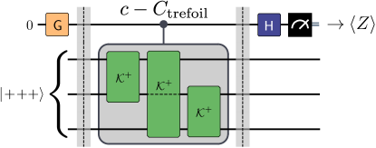
Figure 1: H-test to compute the real and imaginary part of $\mathcal{Z}_{\textrm{trefoil}}=2^{3}\langle+++|C_{\textrm{trefoil}}|+++\rangle$. Setting $G=H$ evaluates the real part $\langle Z\rangle=\textrm{Re}\{\mathcal{Z}_{\textrm{trefoil}}\}/2^{3}$, instead choosing $G=S^{\dagger}H$ returns the imaginary part $\langle Z\rangle=\textrm{Im}\{\mathcal{Z}_{\textrm{trefoil}}\}/2^{3}$.

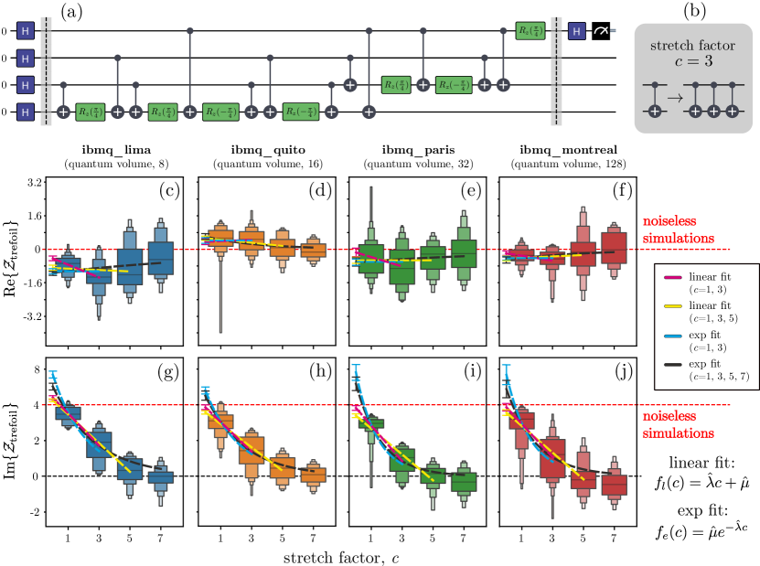
Figure 2: Experimental data for the H-test of the Ising anyon trefoil knot partition function, $\mathcal{Z}_{\textrm{trefoil}}$. (a) H-test circuit for the real part of the calculation, compiled into single qubit rotations and CNOT gates. (b) Final estimates are obtained by zero-noise extrapolation. Stretch factors $c=3,5,7$ are implemented by replacing each CNOT gate with $c$ sequential CNOTs. (c-f) Experimental results for the real part. (g-j) Experimental results for the imaginary part. Experiments were repeatedly executed on four different IBM Quantum backends giving approximately 150 result sets for each backend, all data was collected between May and August 2021. Each panel in (c-j) shows the distribution of the data for different stretch factors (using boxen plots), as well different fits applied to the full set of data. These fits are used to obtain final estimates through extrapolation to $c=0$, we consider linear fits $f_{l}(c)$ and exponential decays $f_{e}(c)$. The values obtained from noiseless simulations are indicated on (c-j) with red dashed horizontal lines. All data shown includes measurement error mitigation.

Error mitigation is used to reduce the effects of noise in the quantum processor Endo et al. (2021); Cirstoiu et al. (2022). We separately mitigate against measurement errors and circuit gate errors.

Measurement errors are addressed by calibrating the measurement confusion matrix and inverting it Endo et al. (2021). Since we only measure a single qubit in the H-test this has very little cost and we apply it to all results presented.

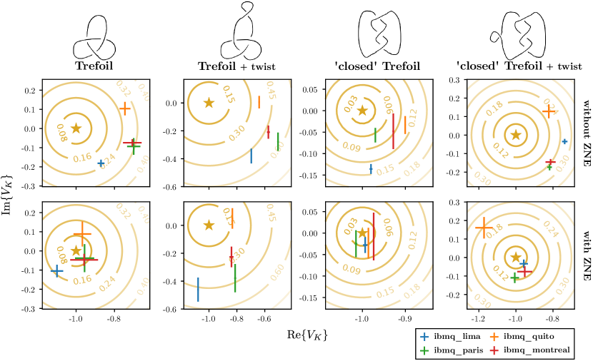
Figure 3: Jones polynomial evaluations $V_{K}(t=i)$ in the complex plane for four topologically equivalent knots from experiments carried out on IBM quantum hardware. Comparing (top row) results without ZNE, CNOT stretch factor $c=1$, to (bottom row) estimates obtained from zero noise extrapolation using a linear fit to $c=1,\,3$. Each panel indicates the exact value $(-1)$ with a star, as well as showing contour lines for the distance from the exact value. The results from four different IBM Quantum devices are plotted with error bars. All results include measurement error mitigation.

To address gate errors we use zero-noise extrapolation (ZNE) Li and Benjamin (2017); Temme et al. (2017); Endo et al. (2021); Bharti et al. (2021); Cirstoiu et al. (2022). In this approach we systematically increase the physical error rate of the gates $\lambda\rightarrow c\lambda$ for $c>1$. By measuring the target observables $\langle O\rangle$ at different stretch factors $c$ we can fit the data to a simple model $\langle O\rangle_{c}\sim f(c)$. ZNE estimates are obtained by extrapolating the fit to zero noise, $f(0)$. Although simple this technique has been shown to be experimentally effective Kandala et al. (2018); Kim et al. (2021); Dumitrescu et al. (2018). Focussing on the CNOT gates as the main source of errors, the error rate in the circuit is increased by replacing each CNOT in the circuit with $c$ consecutive CNOTs Dumitrescu et al. (2018); Giurgica-Tiron et al. (2020); He et al. (2020), Fig. 2(b). In the noiseless case pairs of CNOTs cancel, however in the presence of noise this increases the error rate by discrete stretch factors $c=3,5,7,\ldots$

Experimental data from our evaluations of $\mathcal{Z}_{\textrm{trefoil}}$ is shown as a function of ZNE stretch factor $c$ for the real part in Figs. 2(c-f) and imaginary part in Figs. 2(g-j). Each panel shows the distribution of the different outcomes obtained over our set of IBM Quantum evaluations as a boxen plot  at each $c=1,3,5,7$. The data from different days is pooled together and we fit to the whole data set, this will help average over the time varying errors resulting from drift and different calibrations. Different fits to the data are shown using either all of the $c$ or a subset, e.g. $c=1,3$. The fits we show are either linear or exponential decays towards zero. The final ZNE estimates obtained from the fits are drawn at $c=0$, along with their error bars. Results for the other three knots we consider are shown in appendix C. More details of the fitting procedure and obtaining uncertainties in our ZNE estimates is given in appendix D.

VIII Experimental results for the Jones polynomial

We combine the evaluations of the partition function with the complex proportionality factors $\mathcal{A}(\tau,\omega,n)$ to give the Jones polynomials $V_{K}(t=i)$. Fig. 3 shows the estimates of $V_{K}(t=i)$ obtained for the four different knots from the IBM Quantum processors. Again, we compare estimates with and without zero-noise extrapolation. For our final estimates we use the simplest fit, a linear fit to small $c=1,3$.

In most cases applying ZNE confers a clear benefit to our results. A significant improvement is realised by the smallest case we consider, ‘closed’ trefoil ($C_{K}$ is a 2 qubit unitary). However, the largest case we consider, trefoil+twist ($C_{K}$ is a 4 qubit unitary), shows a much weaker benefit. It is typically expected that error mitigation strategies will decrease the bias of a estimate while increasing its variance Endo et al. (2021) and that is the behaviour we see, with our ZNE estimates lying closer to the target value but having larger error bars.

The four knots we consider are topologically equivalent meaning they all have the same Jones polynomial value $V_{K}(t=i)=-1$. In principle, we would expect all our experimental estimates to be consistent with each other and with $(-1)$, however, as Fig. 3 shows that is not always the case due to errors. To more directly make the comparison Fig. 4 jointly plots the final error-mitigated estimates for the knots, evaluated on ibmq_montreal. We see that three of the four are consistent with each other up to error bars and are clustered together close to $(-1)$, however, the remaining knot Trefoil$+$twist is significantly apart. If we had no prior knowledge of what $V_{K}(t=i)$ should be we may incorrectly conclude that Trefoil$+$twist is topologically distinct from the other knots. However, if we were performing a simpler task, for instance answering whether we think this knot is more likely to be topologically equivalent to the trefoil, $V_{K}(t=i)=-1$, or the unknot, $V_{K}(t=i)=+1$, this noisy estimate may be good enough.

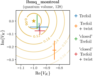
Figure 4: Comparing Jones polynomial evaluations $V_{K}(t=i)$ of four topologically equivalent knots obtained from the ibmq_montreal QPU. Values are plotted in the complex plane. Without noise we would expect all four knots to give the same value $V_{K}(t=i)=-1$, which is indicated with a star. However, errors shift the values we obtain, moving them away from $(-1)$ and causing them to not all overlap with each other. We plot contour lines showing the distance from this exact value. Estimates of $V_{K}(t=i)$ include both measurement error mitigation and zero noise extrapolation using a linear fit to $c=1,\,3$.

IX Related work and $\text{DQC}_{1}$

The authors of Refs. Marx et al. (2010); Göktaş et al. (2019) have used the one-clean qubit model, or $\text{DQC}_{1}$, the ‘one clean qubit’ model, to estimate the Jones polynomial at roots of unity, respectively using nuclear magnetic resonance technology and superconducting quantum processors provided by IBM. The latter work frames their work as a benchmark for noisy quantum computers.

In the quantum protocols used therein, one is interested in estimating the trace of a unitary matrix by using as a resource the maximally mixed state. The $\text{DQC}_{1}$ protocol is identical to the H-test, with the difference that the maximally mixed state is used as a resource instead of a pure state. Operationally, on the circuit model of quantum computation, one would simulate the preparation of the maximally mixed state by averaging over H-tests while uniformly sampling the pure state from the computational basis.

Interestingly, evaluating the Jones polynomial on roots of unity is DQC1-complete for the trace, or ‘Markov’, closure of a braid Shor and Jordan (2007), and is BQP-complete for the closure of a braid with ‘cups’ and ‘caps’, called the ‘Plat’ closure Aharonov and Arad (2011); Kuperberg (2015). These results involve unitary representations of the braid-group generators at particular roots of unity. The braid group acts on strands that are drawn in parallel and generators swap neighbouring strands clockwise and anticlockwise. Their unitary representations can be seen as local unitary gates, which when composed form arbitrary unitary transformations. The exception to universality is for lattice roots of unity.

One would be tempted to conclude from the above that $\text{DQC}_{1}=BQP$, which is not believed to be the case. Alexander’s theorem states that any knot diagram $K$, which can be viewed as the Plat closure $K=P(B)$ of a braid $B$, can be rewritten as the Markov closure of another braid $K=M(B^{\prime})$. Moreover, the braid $B^{\prime}$ can be efficiently obtained with Vogel’s algorithm Birman and Brendle (2005). For a given root of unity, a braid $B$ is represented as a unitary $U_{B}$ and the cups and caps are represented by pure basis states and basis effects KAUFFMAN and LOMONACO (2008). So, $P(B)$ represents a quantum amplitude $\langle\text{cups}|U_{B}|\text{caps}\rangle$, which is estimated with the H-test Aharonov et al. (2009). Also, $M(B^{\prime})$ represents $\text{tr}(U_{B^{\prime}})$ and is obtained by $\text{DQC}_{1}$. The subtle caveat lies in that $B^{\prime}$ in general involves a larger number of strands than $B$ Shor and Jordan (2007). Furthermore, the dimension of $U_{B}$ depends exponentially on the number of strands in $B$. Since both the H-test and $\text{DQC}_{1}$ estimate a quantity up to additive error, this means that, in the worst case, for the same number of samples the additive error in the quantum protocol involving the braid with the larger number of strands will be exponentially worse. One can of course attempt to find a minimal braid representative of $B^{\prime}$ Gittings (2004), i.e. a braid which has the fewest possible number of strands and is topologically equivalent to $B^{\prime}$ after a Markov closure, but this is a hard optimisation problem.

Note that recognising the unknot is in NP $\cap$ co-NP Hass et al. ; Kuperberg (2014), and it is interestingly an open problem whether there exists an algorithm in P for it. Remarkably, a quasipolynomial algorithm was announced for the unknotting problem recently oxM .

X Discussion

In this work we have rigorously demonstrated that we are able to use current quantum hardware to obtain good estimates of Jones polynomials for small knots. Further, by applying zero-noise extrapolation we were able to boost the accuracy of our estimates. In some cases we were able to identify the topological equivalence between the different knots we were looking at.

An obvious way to further improve our results would be to use more sophisticated error mitigation strategies. We employed a simple approach where CNOT gates were multiplied and we made one parameter empirical fits to the data. Other approaches are able generate non-integer stretch the factors, allowing us to acces values of $c$ close to 1 where we would expect simple fits to the noisy observable to hold best. These methods include stretching the control pulses of the hardware in time Kandala et al. (2018) or randomising the insertion of extra CNOTs He et al. (2020). Similarly, we can consider fitting models that are derived from the physical error model of the device Endo et al. (2021) or multi-parameter scalings of the noise rates Otten and Gray (2019). Finally, the most successful applications of error mitigation combine various strategies including zero-noise extrapolation, dynamical decoupling and Pauli twirling Kim et al. (2021).

Before closing, we recall that our setup introduces a standardised bechmark for NISQ processors. Randomly applying Reidemeister moves to specific knots leaves the Jones polynomial invariant. Such a procedure thus gives an efficient way to produce distributions of knots, and therefore stabiliser circuits, for which we know we should obtain the same result. This defines a standardised benchmark for NISQ processors and error mitigation protocols. Tangentially, our work can be generalised to the evaluation of the Jones polynomial at the sixth root of unity, in which case qutrit stabiliser circuits are involved. Finally, one can move beyond NISQ and consider evaluating the Jones polynomial via the unitary representations of the braid group, in which case the quantum amplitudes to which the problem reduces to involve circuits comprising gates from a universal gateset. In this case, evaluating the Jones polynomial for small knots for which the full polynomial is known constitutes a benchmark for the first error corrected quantum computers.

Finally, another general direction for further work would be to adapt this work around the problem of estimating partition functions of families of classical spin models, such as Ising or Potts. In addition, similar benchmarks for NISQ as well as error corrected processors as what we argue for in this work can be defined in terms of classical spin models. More interestingly even, using quantum computers to execute the H-test allows for the exploration of the average case behaviour of problem families whose complexity is known, conjectured, or unknown.

Code and data availability

Code to reproduce the experimental results presented in this paper is available from git . In git repository knu , connected to Ref. Meichanetzidis and Kourtis (2019), we provide a python script knut.py containing functions that, given a planar code for a knot, return the writhe, the Tait number, and the Tait graph.

The experimental data presented in this paper is available from zen .

APPENDIX

Appendix A Knot specifications

Sections II-VI of the main text describe how the calculation of the Jones polynomial (at $t=i$) can be performed on a quantum computer. This process begins with the knot diagram and ends with an $n$-qubit unitary, $C_{K}$, whose complex amplitudes ${}^{\otimes n}\langle+|C_{K}|+\rangle^{\otimes n}$ are evaluated with an H-test. When normalised, these complex amplitudes correspond to the partition function of a Potts model, $\mathcal{Z}_{K}=2^{n}\cdot{}^{\otimes n}\langle+|C_{K}|+\rangle^{\otimes n}$. The Jones polynomial $V_{K}(t=i)$ is linked to these partition functions by a complex proportionality factor $V_{K}=\mathcal{A}(\tau,w,n)\mathcal{Z}_{K}$.

In our experiments on IBM Quantum devices we consider four knots. The knot diagrams, qubit unitaries $C_{K}$ and complex proportionality factors $\mathcal{A}(\tau,w,n)$ for these knots are given in Fig. 5.

The knots we consider are topologically equivalent and all have Jones polynomial $V_{K}(t=i)=-1$. Despite this equivalence the complexity of the circuit unitaries varies, including the number of qubits they act on. In the simplest case $C_{K}$ is a single two qubit unitary. This simplification occurs because of the mapping

followed by applying the identity

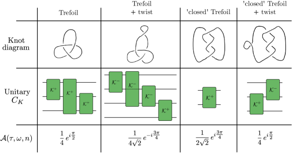
Figure 5: Specification of the knots considered on IBM quantum devixes. The four knots are topologically equivalent and each have Jones polynomial values $V_{K}(t=i)=-1$. For each knot, the knot diagram and related circuit unitary are shown. Additionally, the complex factors linking the circuit amplitude to the Jones polynomial, $\mathcal{A}(\tau,\omega,n)$ are given.

Appendix B Experimental details

The Ising anyon partition functions, $\mathcal{Z}_{K}$, for the four knots described in Appendix A were estimated by running experiments on IBM Quantum processors. Our experiments consisted of repeatedly submitting the quantum computation to a set of different devices over many days between May and August 2021. Here we give additional details on the practical aspects.

The controlled unitaries of the H-tests were compiled into gates using the Qiskit ‘diagonal’ function, which implements the algorithm given in Shende et al. (2006).

Each day during the experiment the real and imaginary H-test circuits were submitted to the IBM Quantum backends ibmq_lima (quantum volume 8), ibmq_quito (quantum volume 16), ibmq_paris (quantum volume 32) and ibmq_montreal (quantum volume 128) a_i ; b_i ; c_i ; d_i . Before each submission the H-test circuits were transpiled for each backend using the TKET python package Sivarajah et al. (2020); pyt (using the default passes for IBM Quantum backends with optimisation level 2). This transpiler is noise-aware, so aspects of the transpiled circuits such as qubit selection will vary day-to-day. ZNE stretched circuits were generated from the transpiled circuit. This ensures that (1) the added CNOT’s were not removed by the transpiler and (2) the ZNE stretched circuits use the same physical qubits. The circuits were batched and submitted to the IBM Quantum cloud service using the circuit submission API. Each submission consisted of four repeated copies of the real and imaginary H-test circuits at each ZNE stretch factors $c=1,3,5,7$. If the submitted circuits failed to execute before the next day the job was cancelled.

Measurement error mitigation was applied to our results using Qiskit’s complete measurement fitter class. The calibration circuits were submitted batched together with our H-test circuits.

The timeline of individual evaluations we obtained for the trefoil knot partition function is shown in Fig. 6. Error bars show the uncertainty due to shot noise on each evaluation. We see that the variability between different days is much larger than the shot noise and will account for most of the uncertainty in our final estimate.

Figure 6: Timeline of evaluations of the (left) real part and (right) imaginary part of $\langle+++|{C}_{\textrm{trefoil}}|+++\rangle$ on four different IBM Quantum backends between May and August 2021. Evaluations shown are without zero-noise extrapolation ($c=1$), but after applying measurement error mitigation. Dashed vertical lines show days that we were able to collect results. Each day consisted of four batched evaluations, which are all individually plotted. All evaluations show error bars for the shot noise uncertainty. Dashed red horizontal lines show the value expected from noiseless simulations, additionally zero is highlighted with a dotted horizontal line.

Appendix C Additional experimental results

In section VII of the main text we present experimental data for the H-test of the Ising anyon trefoil knot partition function. Here we show the experimental results we have for the Ising anyon partition function of the other three knots – Fig. 7 presents the data for the trefoil+twist knot, Fig. 8 for the ‘closed’ trefoil in knot and Fig. 9 for the ‘closed’ trefoil+twist. Exponential fits to the trefoil+twist data did not all converge so we only show linear fits in that case.

Appendix D ZNE fits and uncertainties

We carry out zero-noise extrapolation fits to data sets where we have pooled together repeated QPU executions. For concreteness consider the $c=1,3,5,7$ exponential fit to $\textrm{Re}\{\mathcal{Z}_{\textrm{trefoil}}\}$. At each $c$ we have approximately 150 separate evaluations from repeated executions on different days, the exact number of repeats varies by device depending on how many job submissions were successful, for simplicity let us have exactly 150 repeats. We can label these separate estimates of $\textrm{Re}\{\mathcal{Z}_{\textrm{trefoil}}\}$ as $y_{c\,t}$, for $c=1,3,5,7$ and $t=1,\ldots,150$. We fit the full dataset $y_{c\,t}$ to $f_{e}(c)=\mu e^{\lambda c}$ using the scipy.optimise.curve_fit function.

Means and uncertainties for the fitting parameters are obtained by bootstrapped resampling. We carry out 50,000 resamples of our data $y_{c\,t}$, where at each $c$ we independently draw samples of size 150 over $t$ with repeats. Each resample is fit to $f_{e}(c)$ giving estimates of the fitting parameters $\mu_{i}$ and $\lambda_{i}$ for $i=1,\ldots,50000$. The mean estimates of the fitting parameters $\hat{\mu}$ and $\hat{\lambda}$ are taken as the mean of the $\mu_{i}$ and $\lambda_{i}$. Uncertainties shown on the fitting parameters in Fig. 2 are 2$\times$ the standard deviation of the $\mu_{i}$. These uncertainties are propagated to the Jones polynomial estimates to give the error bars in Fig. 3 and Fig. 4. We note that independently resampling over $t$ at each $c$ scrambles experiments that were carried out at the same time. We compared it to the case where we resample tuples ($y_{1\,t}$, $y_{3\,t}$, $y_{5\,t}$, $y_{7\,t}$) over $t$, but find no difference in the results.

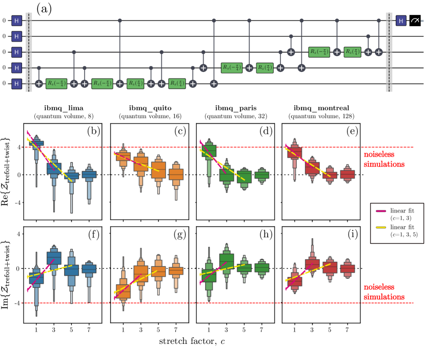
Figure 7: Experimental data for the Ising anyon trefoil with a twist knot partition function, $\mathcal{Z}_{\textrm{trefoil+twist}}$. (a) H-test circuit for the real part of the calculation, compiled into single qubit rotations and CNOT gates. (b-e) Experimental results for the real part. (f-i) Experimental results for the imaginary part. Experiments were repeatedly executed on four different IBM Quantum backends giving approximately 150 result sets for each backend. Each panel in (b-i) shows the distribution of raw data for different stretch factors (boxen plots), as well different linear fits to the data. These fits are used to obtain final estimates through extrapolation to $c=0$. The values obtained from noiseless simulations are indicated on (b-i) with red dashed horizontal lines. All data shown includes measurement error mitigation.

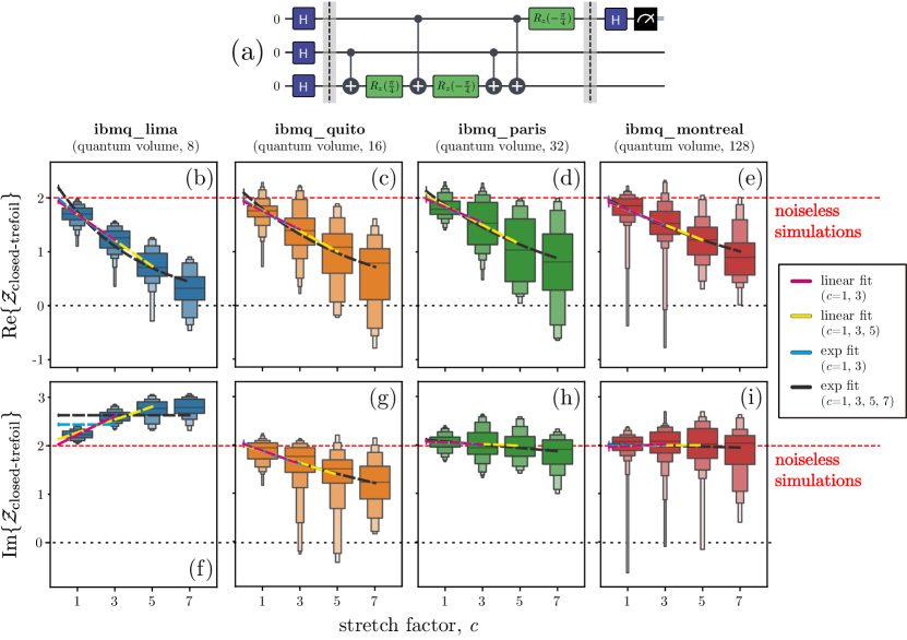
Figure 8: Experimental data for the Ising anyon ‘closed’ trefoil knot partition function, $\mathcal{Z}_{\textrm{closed-trefoil}}$. (a) H-test circuit for the real part of the calculation, compiled into single qubit rotations and CNOT gates. (b-e) Experimental results for the real part. (f-i) Experimental results for the imaginary part. Experiments were repeatedly executed on four different IBM Quantum backends giving approximately 150 result sets for each backend. Each panel in (b-i) shows the distribution of raw data for different stretch factors (boxen plots), as well different linear and exponential fits to the data. These fits are used to obtain final estimates through extrapolation to $c=0$. The values obtained from noiseless simulations are indicated on (b-i) with red dashed horizontal lines. All data shown includes measurement error mitigation.

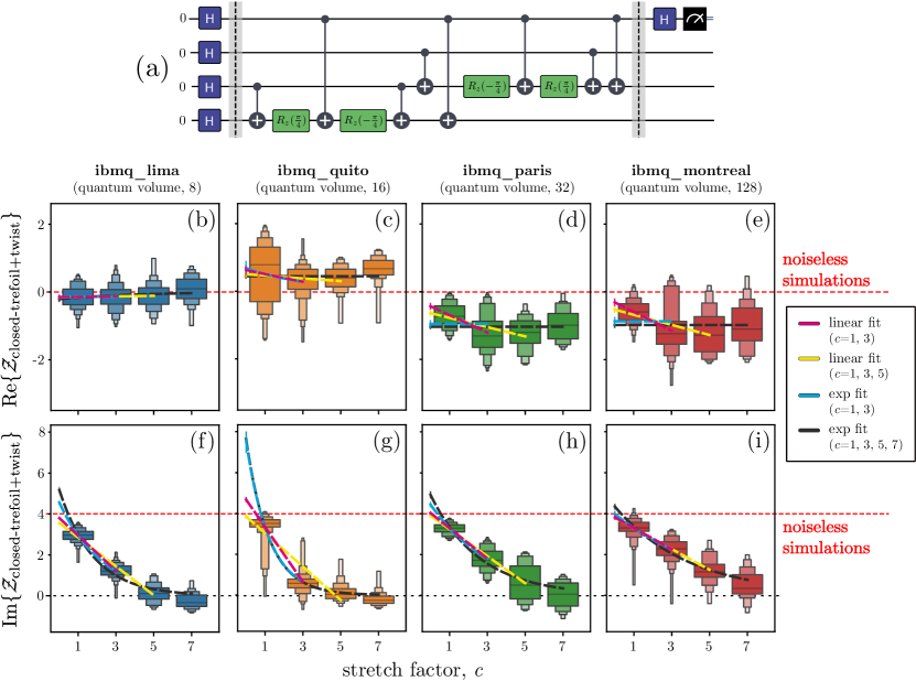
Figure 9: Experimental data for the Ising anyon ‘closed’ trefoil with a twist knot partition function, $\mathcal{Z}_{\textrm{closed-trefoil+twist}}$. (a) H-test circuit for the real part of the calculation, compiled into single qubit rotations and CNOT gates. (b-e) Experimental results for the real part. (f-i) Experimental results for the imaginary part. Experiments were repeatedly executed on four different IBM Quantum backends giving approximately 150 result sets for each backend. Each panel in (b-i) shows the distribution of raw data for different stretch factors (boxen plots), as well different linear fits to the data. These fits are used to obtain final estimates through extrapolation to $c=0$. The values obtained from noiseless simulations are indicated on (b-i) with red dashed horizontal lines. All data shown includes measurement error mitigation.