Numerical study of the Transverse Diffusion coefficient for a one component model of plasma

Abstract

In this paper we discuss the results of some Molecular Dynamics simulations of a magnetized One Component Plasma, targeted to estimate the diffusion coefficient $D_{\perp}$ in the plane orthogonal to the magnetic field lines. We find that there exists a threshold with respect to the magnetic field strength $|\vec{B}|$: for weak magnetic field the diffusion coefficients scales as $1/|\vec{B}|^{2}$, while a slower decay appears at high field strength. The relation of this transition with the different mixing properties of the microscopic dynamics is investigated by looking at the behavior of the velocity auto correlation.

The diffusion process is well understood for stochastic motions (see Ref. [3]), that are supposed to mimic the behaviour of a chaotic dynamical system. Many questions are instead left open in the study of the diffusive properties of a system which is in a partially ordered state (see for example Ref. [27]). A central issue, as regards magnetized plasma confinement, is the diffusion of charged particles in the direction perpendicular to the magnetic field lines. A widely accepted law, predicting that the transversal diffusion $D_{\perp}$ coefficient is proportional to the inverse of the square of the magnetic field strength $|\vec{B}|$, was proposed more than 50 years ago( see Ref. [21]). Being based on kinetic theory, this law is expected to hold whenever the microscopic dynamics is chaotic. However, as the magnetic field $|\vec{B}|$ is increased, a partially ordered state seems to set in (see Refs. [7, 9]), at least for a pure electron plasma. Our purpose was to investigate the consequences (if any) of this transition on the diffusion process. So we have performed Molecular Dynamics simulations of a magnetized one component plasma, that is a set of mutually interacting electrons subject to a constant external magnetic field. We estimate the diffusion coefficient $D_{\perp}$ in the plane orthogonal to the field, for different values of the magnetic field strength $|\vec{B}|$. We find that the kinetic law holds for low $|\vec{B}|$, when the microscopic dynamics is chaotic. But as the magnetic field grows the diffusion coefficient seems to saturate to a plateau, while the microscopic state turns to a partially ordered one.

1 Introduction

In the years Sixties there was a great exchange among research groups of plasma physics and of dynamical systems, as both were interested in the study of the $1\tfrac{1}{2}$ Hamiltonian system that can represent the magnetic field lines; see Ref. [12] for a broad historical overview. In more recent years, another point of connection have become the study of diffusion process in the phase space, see Ref. [3]. It has been shown that if the dynamics is not fully chaotic, then the process of diffusion in the phase space can be “not normal”, i.e., the mean square displacement doesn’t necessarily grow linearly in time: the process is called super diffusive if the growth is faster than linear, or sub diffusive otherwise; for a review see [27]. In both cases there is no widespread agreement of the correct definition of the diffusion coefficient to be adopted.

Figure 1: Diffusion coefficient $D_{\perp}$ perpendicular to the magnetic field versus $\beta$, computed by MD simulations. Circles are the numerical results, while the solid line is the plot of the function $D_{\perp}=\frac{\gamma A}{\gamma^{2}+\beta^{2}}$, with $\gamma=0.168$ and $A=9.9$. Such values are obtained from the auto correlation of the electron velocities, as explained in the text. The broken line is the plot of the function $D_{\perp}\simeq\beta^{-0.7}$, corresponding to the law found in paper [13].

Now, as it will be shown below, the equations of motion for a single electron in a one component plasma subject to an external constant magnetic field $\vec{B}$ can be recasted in a dimensionless form, in which the only parameter appearing is the ratio $\beta=\sqrt{4\pi}\omega_{c}/\omega_{p}$ among the cyclotron frequency $\omega_{c}=eB/mc$ and the plasma frequency $\omega_{p}=\sqrt{4\pi ne^{2}/m}$ (in the c.g.s. system); here $n$ is the particle density and $e$ the electronic charge. The parameter $\beta$ measures the relative strength the magnetic Lorentz force acting on a single electron, with respect to the electrostatic force due to all other electrons. In the limit of $\beta\to+\infty$ the equations of motions decouple and the system reduces (formally) to a set of independent electrons in a constant magnetic field, i.e., to an integrable system.

So, it can be conjectured that for high magnetic field strength, the dynamics will not be fully chaotic, (see papers [7] and [9]), and that the diffusion process in phase space may be “anomalous”. Actually, it is impossible for us to study numerically such process, and we limit ourselves to study the diffusion of the electrons in the physical space. To this end we study the diffusion coefficient, defined as usual (see for example Ref. [1]) by

$$D_{\perp}=\lim_{t\rightarrow\infty}\frac{\langle\left|\Delta\vec{x}_{\bot}\right|^{2}\rangle}{4t}$$ (1)

being $\left|\Delta\vec{x}_{\bot}\right|^{2}$ the mean displacement, in the plane perpendicular to the magnetic field, of the electrons from their initial positions, while $\langle\cdot\rangle$ should be the phase average. Instead in this paper, following a common attitude, averages will be always taken as time averages along the orbits. We have not investigated the relations between the two averages.

As regards physical applications, small values of $D_{\perp}$ are important for the purpose of plasma confinement in fusion devices. This is another reason to investigate in which regime the diffusion coefficient is small.

Another dimensionless parameter which characterize the state of a plasma is the coupling parameter $\Gamma=e^{2}/(ak_{B}T)$, where $a$ is the inter particle spacing (related to the particle density $n$ by the relation $a=n^{1/3}$), $T$ the plasma temperature and $k_{B}$ as usual the Boltzmann constant. So defined, $\Gamma$ is the ratio among the mean coulomb energy of a couple of nearest particles, and the mean kinetic energy. The weak coupling regime is then defined by $\Gamma<1$ and the strong coupling regime by $\Gamma\geq 1$. Up to now, because of the reasons explained in the following, Molecular Dynamics (MD) simulations have been performed mainly in the strongly coupled case, while the weakly coupled regime have been addressed mostly by kinetic theory.

In literature it is possible to find different estimates for the diffusion coefficient. The oldest one (see Ref. [21]) predicting the scaling law $D_{\perp}\propto\beta^{-2}$, is obtained in the frame of the kinetic theory, in the weak coupling regime. However, other different theories have been proposed in the years, each giving a different law for the dependence of the diffusion coefficient $D_{\perp}$ on the parameter $\beta$. A few of them are summarized in Table 1 on page 135003-2 of Ref. [22]; another one is percolation theory (see Refs. [17, 18, 13]), which predicts a scaling like $\beta^{-0.7}$. This law is in the closest agreement with our results. It was brought to our attention by an anonymous referee that we warmly thank.

But none of the proposed theories is based on the loss of chaoticity in the Newtonian microscopic dynamics. Also the numerical works found in literature fail to address this point. In fact, up to now, the behaviour of the diffusion coefficient have been investigated by MD mostly in the unmagnetized case, see for instance Refs. [10, 24, 4]. The magnetized case was studied in Ref. [22], but only in the strong coupling regime: at the smallest value $\Gamma=1$ a transition at $\beta\approx 1$ in the behavior of $D_{\perp}$ was observed, but the origin of such a transition was not discussed. A similar transition was observed also in two more recent works [2] and [25], where the diffusion coefficient was studied numerically for $\Gamma$ down to $0.1$. However, those works were based on a so-called Particle-Particle Particle-Mesh ($P^{3}M$) code, which is a sort of hybrid between a kinetic and a MD code. We think that such method is not suited to study the chaoticity of the microscopic dynamics. More on the connections between our results and the cited paper will be said in the conclusions.

So in this paper we perform a fully MD simulation for different values of $\beta$ for a system of $N=4096$ electrons, for a fixed value of $\Gamma=0.1$, which is the smallest value we were able to manage. The aim is to verify for what value of $\beta$ the transition in the behavior of $D_{\perp}$ occurs, and to observe the chaoticity of the dynamics, by computing the time auto correlation of the transverse particle velocity.

In Section 2 we describe the model and the numeric algorithm used, in Section 3 the numerical results are reported while in Section 4 the conclusions follow.

2 The model and the numerical scheme

The system we are considering is called in the literature a one component plasma and it consists of a number $N$ of electrons in a cubic box of side $L$ with periodic boundary conditions, the electrons being subject to mutual Coulomb interactions, and to an external constant magnetic field $\vec{B}=B\vec{e}_{z}$ ($\vec{e}_{z}$ is the unit vector directed along the $z$ axis). The density is then defined by $n=N/L^{3}$. This is considered a model of a plasma as the positive ions are supposed to constitute a uniform neutralizing background.

If $t$ denotes time and $\vec{x}_{i}$ the position of the $i$-th electron (with $i=1,\dots,N$), we define dimensionless variables

$$\vec{y}_{i}=a^{-1}\vec{x}_{i},\quad\tau=\omega_{c}t\ ,$$ (2)

by rescaling distances with the inter particle spacing $a=n^{-1/3}$ and time with the cyclotron frequency $\omega_{c}$. Using such variables, the equations of motion for the $i$-th electron read

$$\frac{d^{2}{\vec{y}}_{i}}{d\tau^{2}}=\vec{e}_{z}\times\frac{{d\vec{y}}_{i}}{d\tau}+\frac{1}{\beta^{2}}\vec{E}(\vec{y}_{i})$$ (3)

where $\vec{E}(\vec{y}_{i})$ is the electric field acting on $i$-th electron due to all other charges. The electric field of a periodic system of charges can be computed via the Ewald formula (see for example Ref. [14]),

$$\begin{split}&\vec{E}(\vec{y}_{i})=\\ &\sum_{\vec{l}}\sum_{j=1}^{N}\frac{\vec{y}_{ij\vec{l}}}{|\vec{y}_{ij\vec{l}}|^{3}}\left[\operatorname{erfc}({\alpha}|\vec{y}_{ij\vec{l}}|)+\frac{2\alpha|\vec{y}_{ij\vec{l}}|}{\sqrt{\pi}}\exp(-{\alpha}^{2}{|\vec{y}_{ij\vec{l}}|}^{2})\right]\\ &+\frac{4\pi}{N}\sum_{\vec{q}\neq 0}\sum_{j=1}^{N}\frac{\vec{q}}{q^{2}}e^{-q^{2}\!/4{\alpha}^{2}}\sin(\vec{q}\cdot\vec{y}_{ji}),\qquad\alpha=\sqrt{\pi}N^{-1/6}\\ \end{split}$$ (4)

where $\vec{l}$ is a triplet of integers denoting the position of an image cell, while $\vec{q}$ is a vector in the reciprocal lattice, i.e. is defined by $\vec{q}=2\pi\vec{n}/L$ with $\vec{n}$ an integer vector, and finally we have defined $\vec{y}_{ij\vec{l}}=\vec{y}_{i}-\vec{y}_{j}+\vec{l}\sqrt[3]{N}$. The two series are truncated as to assures a relative error below $10^{-7}$, which is smaller than the relative error of the energy conservation in a single numerical step.

Of the two dimensionless parameters of the problem, only $\beta$ appears into the equations of motion. The parameter $\Gamma$ enters through the choice of the initial data: in fact, while the positions are extracted from a uniform distribution, the velocities are taken from a Maxwell distribution, and the temperature is uniquely determined by $\Gamma$. With this choice, at the beginning of each simulation, the system is out of equilibrium: so there is a drift of the kinetic energy, and the system reaches a different, random, temperature. In order to fix the temperature to the desired value, we operate in this way: after extracting the initial values, we let the system evolve until equilibrium is reached, i.e. until the kinetic energy appears to stabilize. We then generate new velocities again with a Maxwell distribution at temperature $T$, and repeat the process until the kinetic energy appears to be constant and close to the chosen value.

The equations (3) were integrated using a symplectic splitting algorithm (see for example Ref. [16]). The total Hamiltonian

$$H=\frac{1}{2}\sum_{k}\Big{(}\vec{p}_{k}+\frac{1}{2}\vec{e}_{z}\times\vec{y}_{k}\Big{)}^{2}+\frac{1}{\beta^{2}}V(\vec{y}_{1},\ldots,\vec{y}_{N})\ ,$$ (5)

where $V(\vec{y}_{1},\ldots,\vec{y}_{N})$ is the Coulomb potential of the electrons computed according the Ewald prescription, was split as $H=H_{1}+H_{2}$ where

$$H_{1}\stackrel{{\scriptstyle\mathrm{def}}}{{=}}\frac{1}{2}\sum_{k}\Big{(}\vec{p}_{k}+\frac{1}{2}\vec{e}_{z}\times\vec{y}_{k}\Big{)}^{2}\ ,\quad H_{2}\stackrel{{\scriptstyle\mathrm{def}}}{{=}}V(\vec{y}_{1},\ldots,\vec{y}_{N})\ .$$ (6)

Now, denoting by $\Phi^{t}_{1}$ the flow determined in the phase space by the Hamiltonian $H_{1}$ and by $\Phi^{t}_{2}$ the one due to the Hamiltonian $H_{2}$, the integration algorithm is obtained simply by composition $\Phi\stackrel{{\scriptstyle\mathrm{def}}}{{=}}\Phi^{\delta t/2}_{1}\circ\Phi^{\delta t}_{2}\circ\Phi^{\delta t/2}_{1}$, where $\delta t$ is the time step. Such time step was chosen so that the energy conservation was better then a part over $10^{4}$ in all the simulations. In particular we choose $\delta t=2\pi C(\beta)\,10^{-4}$, where the factor $C(\beta)$ is taken equal to $\beta$ for $\beta<1$, and costant equal to 1 for larger $\beta$. In figura 2 we report the relative error of the energy conservation as a function of the number of integration step, for a tipical run. The number of step used was $4\,10^{6}$ for $\beta\leq 2.5$, four times this number for $\beta$ larger.

Figure 2: Relative error of the energy conservation as a function of the number of integration steps. Data refers to a case with $\beta=1$ and $N=4096$ particles.

In MD simulations the choice of the number $N$ of particles is always an issue, all the more in the context of a weakly coupled Plasma. For a very rough estimation, we made the following considerations: the fundamental cell of the simulation should have a side larger than the Debye length $\lambda_{D}$, which in our units reads $\lambda_{D}=\sqrt{1/\Gamma}$. The first of (2) implies that $L=N^{1/3}$, so that the requirement $L>\lambda_{D}$ in our units becomes $N>\Gamma^{-3/2}$. As the Coulomb force is long range, the computational cost scales as a power of $N$. With a clever use of the Ewald summation formula, see Ref. [23], the computational cost scales (asymptotically) as $N^{3/2}$. So we cannot afford to choose a value much bigger than $N=4096$. In any case, for $\Gamma=0.1$ our constraint reads $N>32$ and so with our choice of $N=4096$ we have $L\simeq 5\lambda_{D}$.

Another interesting length scale which appears in the problem is the Larmor radius $r_{l}$, i.e., the gyration radius of the electrons determined by the magnetic Lorentz force due to the external magnetic field $B$. A simple computation shows that one has $r_{l}/L=\sqrt{2/\Gamma}/\beta N^{1/3}$. For the smallest value of $\beta$ used in our computations, i.e. $\beta=0.25$, the Larmor radius is slightly larger than the side of the simulation cell, because one gets $r_{l}\simeq 1.1L$. Instead $r_{l}$ turns out to be well below the Debye length, for the largest value of $\beta=10$.

3 Results

We recall that the transverse diffusion coefficient is defined by (1), where

$$\left|\Delta\vec{x}_{\bot}\right|^{2}\stackrel{{\scriptstyle\mathrm{def}}}{{=}}\frac{\sum_{k}\Big{(}|x_{k}(t)-x_{k}(t_{0})|^{2}+|y_{k}(t)-y_{k}(t_{0})|^{2}\Big{)}}{N}$$ (7)

is the mean particles displacement in the plane orthogonal to the magnetic field $\vec{B}$ (we recall that the latter was taken directed as the $z$–axis) and the brackets denote the time average along the orbit. To estimate this quantity we proceed as follows.

Let $\delta t$ be the integration step and $M_{tot}$ the total number of integration steps. Let also $j$ be an integer smaller than a fixed fraction $M^{\prime}$ of $M_{tot}$ (we take one sixteenth), then the time averages of $\langle\left|\Delta\vec{x}_{\bot}\right|^{2}\rangle$ at time $t_{j}=j\delta t$ were computed as

$$\langle\left|\Delta\vec{x}_{\bot}\right|^{2}\rangle(t_{j})=\frac{1}{M}\sum_{h=1}^{M}\left(\frac{1}{N}\sum_{k=1}^{N}\Big{(}|x_{k}(t_{h+j})-x_{k}(t_{h})|^{2}+|y_{k}(t_{h+j})-y_{k}(t_{h})|^{2}\Big{)}\right)\ ,$$ (8)

where $M=M_{tot}-M^{\prime}$. After plotting $\langle\left|\Delta\vec{x}_{\bot}\right|^{2}\rangle$ as a function of time, we fit the tail with a straight line whose angular coefficient (divided by four) is an estimate of the diffusion coefficient. The values computed in such way can be found in Table 1 (second entry).

Table 1: Values of the diffusion coefficient $D_{\perp}$, toghether with the values of the parameter $A$, $\omega$ and $\gamma$ appearing in the fit of velocity auto correlation.

$\beta$	$D_{\perp}$$~{}^{\mathrm{a}}$	$D_{\perp}$$~{}^{\mathrm{b}}$	$A$	$\omega$	$\gamma$
0.25	18.1	17.9	9.90	0.253	0.169
0.50	5.61	5.91	9.85	0.506	0.169
0.75	2.68	2.83	9.80	0.754	0.167
1.00	1.56	1.63	10.1	1.01	0.164
1.25	1.03	1.07	9.95	1.258	0.166
2.00	0.428	0.434	9.90	2.022	0.165
2.50	0.327	0.342	9.75	2.518	0.171
4.00	0.212	0.200	10.0	4.046	0.168
5.00	0.188	0.184	10.35	5.035	0.164
10.0	0.133	0.146	10.30	10.06	0.157

$~{}^{\mathrm{a}}$ computed from the linear fit of the tail of function (8).

$~{}^{\mathrm{b}}$ computed from the velocity correlation by formula (9).

The whole set of our plots (in log–log scale) can be found in figure 3; as usual, they display a diffusive (linear) behaviour only after a certain time (the so called “ballistic jump”). So we also restricted the sets of points to the latter time window to exclude small times.

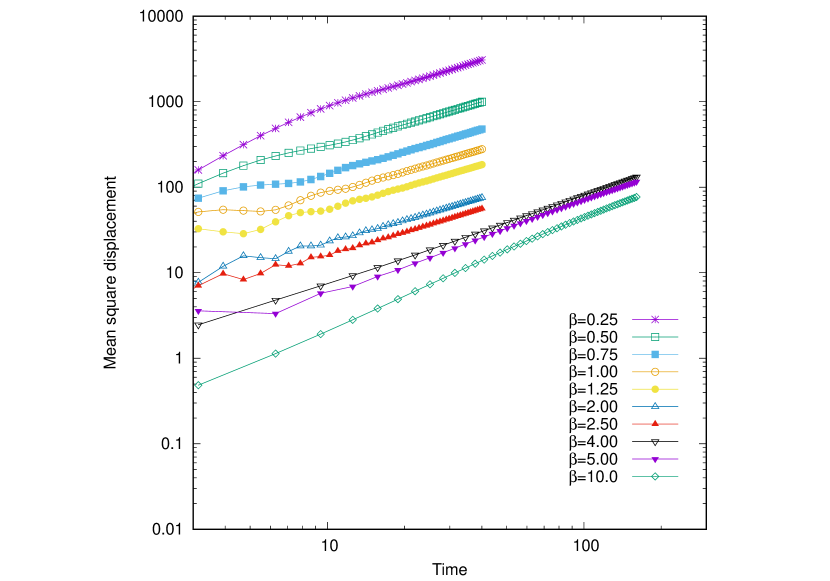
Figure 3: The average square displacement as a function of time. It is interesting to observe the initial non diffusive behaviour, which becomes more evident as $\beta$ is increased.

The results of our computations are summarized in figure 1. There, in logarithmic scale, the numerically computed values of the coefficient $D_{\perp}$ are reported (full circles) as a function of $\beta$. All the simulations were performed at the same value of $\Gamma=0.1$. The solid line is the plot of the function $D_{\perp}=\frac{\gamma A}{\gamma^{2}+\beta^{2}}$, with $\gamma=0.168$ and $A=9.9$. It can be checked that this function agrees very well with the numerical results for $\beta<2$. We remark that, for small values of $\gamma$, this function decrees as $\beta^{-2}$, i.e., for $\beta<2$, the computed values of $D_{\perp}$ agrees with the prediction of the kinetic theory. But by further increasing the magnetic field above a value about $2$, the plot shows a “knee”: the diffusion coefficient appears to obey a different law. These results are in agreement with figure 5(a) of Ref. [25]. Notice that for such value of $\beta$, the Larmor radius $r_{l}$ is slightly smaller than Debye length.

Figure 4: Velocity auto correlation $\langle\vec{v}_{\perp}(t)\cdot\vec{v}_{\perp}(0)\rangle$, as a function of time, for different values $\beta=0.5$, $\beta=1.25$, $\beta=2.5$ and $\beta=5$, of the magnetic field (circles), together with a best fit by a damped oscillation $A\cos\omega te^{\gamma t}$ (solid line). The values of the parameter $A$, $\gamma$ and $\omega$ are reported in each panel. The fit is very good either below and above $\beta=2$. Notice that $A$, $\gamma$ are essentially independent from $\beta$, while $\omega$ agrees well with the cyclotron frequency $\omega_{c}$.

The law $D_{\perp}=\frac{\gamma A}{\gamma^{2}+\beta^{2}}$, was not obtained by interpolation, but by the use of the following argument. Let us introduce the velocity auto correlation $\langle\vec{v}_{\perp}(t)\cdot\vec{v}_{\perp}(0)\rangle$ where $\vec{v}_{\perp}$ in the component of the mean particles velocity transverse to the magnetic field, and the brackets denote the time averages along the orbit. Then the diffusion coefficient can be expressed (see the handbook [26]) as

$$D_{\perp}=\frac{1}{2}\int_{0}^{+\infty}\langle\vec{v}_{\perp}(t)\cdot\vec{v}_{\perp}(0)\rangle\,\mathrm{d}t$$ (9)

whenever the velocity auto correlation decays at $t\to+\infty$ fast enough. Let us introduce a function $f(t)$ to describe this decay by setting

$$\langle\vec{v}_{\perp}(t)\cdot\vec{v}_{\perp}(0)\rangle\simeq\langle\vec{v}_{\perp}(0)\cdot\vec{v}_{\perp}(0)\rangle\cos(\omega_{c}t)f(t)\ .$$ (10)

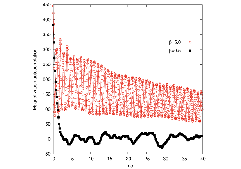
Figure 5: Autocorrelation of the magnetization (along the magnetic field direction) as a function of time, for two different values $\beta=0.5$ (square) and $\beta=5$ (circles) of the magnetic field. Notice that, for a field below the threshold the auto correlation vanishes very fast, while, above the threshold, autocorrelation vanishes eventually on a totally different time scale.

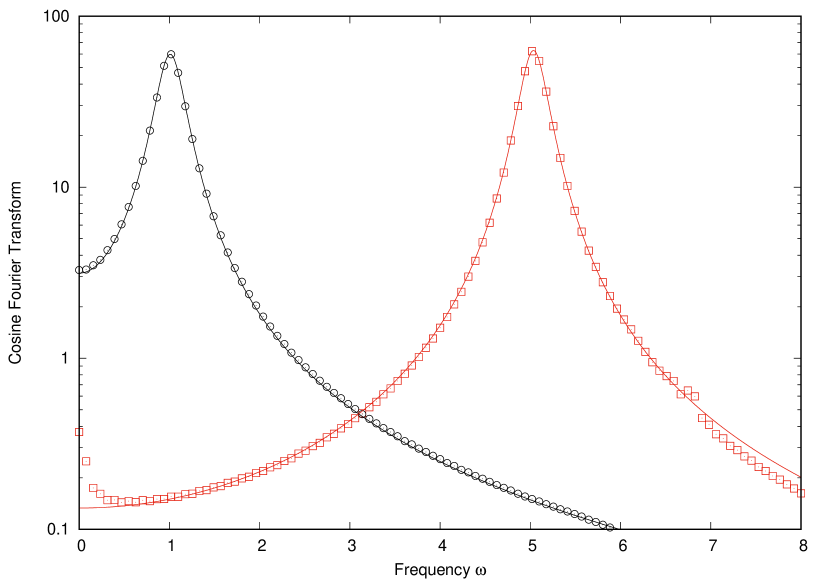
Figure 6: Spectrum of the velocity as a function of $\omega$ in semi logarithmic scale, for two different value of $\beta=0.5$ (circle) and $\beta=5$ (square). The continuous lines are the Fourier transform of the damped oscillation $2Ae^{-\gamma t}\cos\omega t$. For $\beta=1.0$ the slope of the spectrum vanishes at $\omega=0$; for $\beta=5$ the slope remains different from zero. This latter case hints to a decay of the velocity auto correlation as $1/t^{2}$ for $t\to+\infty$ (see text).

Recalling the electronic dynamics, we expect that, due that the gyration along the magnetic field lines alone, $\langle\vec{v}_{\perp}(t)\cdot\vec{v}_{\perp}(0)\rangle$ would oscillate with the cyclotron frequency $\omega_{c}$. However, the electric interaction between the electrons instead determines a loss of coherence of the electronic motion, and thus the decaying to zero of the auto correlation. A common choice is to consider an exponential decay, and thus $f(t)=2Ae^{-\gamma t}$, where $\gamma$ is a parameter representing the inverse of the decorrelation time. Then formula (9) gives exactly $D_{\perp}=\frac{\gamma A}{\gamma^{2}+\beta^{2}}$.

In figure 4 the velocity auto correlation is plotted as a function of time, for different values of $\beta$, either above and below the threshold $\beta=2$. As one can check the law (10) is nicely agreed. From the values reported in table 1, one finds that the parameters $A$ and $\gamma$ are quite independent from $\beta$, while $\omega$ turns out to be very close to the cyclotron frequency $\omega_{c}$ (equal to $\beta$ in our units) as expected. So, taking average values $A=9.9$ and $\gamma=0.168$, and $\omega=\omega_{c}$ the values of the diffusion coefficient $D_{\perp}$ obtained by numerical computations can be recovered from formula (9).

Now, a peculiar fact happens. In fact, while formula (10) appears to be in very good agreement with the velocity auto correlation plots for all the values of $\beta$ considered, the formula $D_{\perp}=\frac{\gamma A}{\gamma^{2}+\beta^{2}}$ is valid only below a threshold $\beta_{cr}\simeq 2$. This notwithstanding, if we compute the time integral numerically and inject it into formula (9), the resulting values of $D_{\perp}$ agree very well with those found using linear regression, as one can check from the Table 1 comparing the values reported in the second and third column. Notice that, when computing the integral appearing formula (9), one has to truncate the integral to an upper limit $t_{max}$ chosen carefully, i.e., not to large, otherwise the numerical errors introduced in computing the auto correlation $\langle\vec{v}_{\perp}(t)\cdot\vec{v}_{\perp}(0)\rangle$ spoil the result.

A possible explanation of this transition when passing from a weakly magnetized to a strongly magnetized regime can be given in the spirit of the paper [9], were it was surmised that at low $\beta$ the plasma is in a fully chaotic regime, but as $\beta$ is increased a transition to a partially ordered regime occurs.

It was shown in that paper how, in such a partially ordered regime, a perturbation theory could apply by adapting the Hamiltonian perturbation theory developed for system of interest in statistical mechanisc (see for example Refs. [5, 8, 15, 11]) to the case of plasma. The idea is that, in the thermodynamical limit, one cannot controll the adiabatic invariants along each individual trajectory (in the phase space), but it is instead possible to controll their auto correlations with respect to an invariant measure, showing that they vanish exponentially slow in the perturbative parameter. Notice that, in virtue of the linear response theory, such auto correlations correspond often to important physical observables.

In the above mentioned paper [9], it was considered the case of the component $M$ of the magnetization along the magnetic field $\vec{B}$, defined (as usual) as

$$M\stackrel{{\scriptstyle\mathrm{def}}}{{=}}\frac{e}{2mc}\frac{1}{N}\sum_{k}(\vec{v}_{k}\times\vec{x}_{k})_{z}\ .$$ (11)

Notice that, the auto correlation $\mathcal{C}_{M}(t)\stackrel{{\scriptstyle\mathrm{def}}}{{=}}<M(t)M(0)>$ is an important quantity because, according the linear response theory, its Fourier transform $\hat{\mathcal{C}}_{M}(\omega)$ gives the magnetic susceptibility $\chi(\omega)$ at the frequency $\omega$ (see for example Refs. [20, 19] or the Appendix B of Ref. [6]).

In our case, the behavior the auto correlation is different below and above the threshold. This is shown in Figure 5: for low magnetic field the auto correlation relaxes to zero, while for high magnetic field it keeps oscillating and eventually vanishes on a totally different time scale. So the magnetizazion could be considered an adiabatic invariant of the system, thus implying that the dynamics remains partially correlated for long times.

A similar mechanism could be at work also in the case of the velocity auto correlation, even if from our plots this is not as evident as in the case of the magnetization. In fact, a clue can be obtained by looking at the spectrum of the velocity auto correlation, i.e., at their cosine Fourier transform, as shown in figure 6 (in semi logarithmic scale). Notice that $D_{\perp}$ is simply half the value of the spectrum at $\omega=0$.

For $\beta=0.5$ the slope of the spectrum seems to vanish at $\omega=0$. As the spectrum is an even function of the frequency this is coherent with the behavior of a smooth function. Instead, for $\beta=5$, the spectrum slope seems to remain (negative and) different from zero at $\omega=0$. Now, it can be very easily shown that, by denoting with $\hat{f}(\omega)$ the Fourier cosine transform of the function $f(t)$ then, for $t\to+\infty$, one has $f(t)=\frac{2}{\pi}\frac{1}{t^{2}}\left(-\hat{f}^{\prime}(0)+o(1)\right)$, if all the derivatives of $\hat{f}(\omega)$ up to the second one are integrable. So it seems that in our data on the velocity auto correlation, there is a small component which decays very slowly (i.e., as $t^{-2}$) to zero. Nevertheless such a component gives a very big contribution to the diffusion coefficient (more then the double of the one due to the exponentially decreasing part $2Ae^{-\gamma t}\cos\omega t$).

In any case, at the moment, it is not clear, for what reason, in a less chaotic regime, the diffusion coefficient apparently decreases, as a function of $\beta$, at a slower rate with respect to the fully chaotic regime.

4 Final considerations

In this work we performed MD simulations of a magnetized electron gas, also called a One Component Plasma. We have shown that such a system shows a transition between two different regimes as the value of the parameter $\beta$ is raised above a critical threshold of about $2$.

The transition occurs both on a macroscopic level, with a change in the diffusive behavior, and on a microscopic level as well: when the parameter is raised, the system passes from a chaotic state to a partially ordered one. This is the main finding that we have pointed out, and is a rather new phenomenon, only remotely addressed in the literature, up to now. As a matter of fact a similar result, for what concerns the behavior of the diffusion coefficient, was published quite recently in Ref. [25]. But the authors tried to explain this phenomenon in the framework of the kinetic theory, looking at the behavior of the particles during the “collisions”. We refrain from this approach, and we try to discuss it according to the ergodic theory of dynamical system, using its standard tools. In particular, our aim is to understand if the dynamics is truly chaotic or not, and, in this latter case, what are the consequence for what concerns the macroscopic quantity characterizing the plasma.

As regards the direct consequences of our results on plasma physics, a strong objection may be raised on the dependence, we have not explored, of the results on the number of particles $N$. In particular, in Ref. [25] it was claimed that a few hundred particles are sufficient in the low $\beta$ regime, but for high $\beta$ a huge number of particles (above $10^{6}$) is needed. In particular, they show that the value of the diffusion coefficient slowly decreases as $N$ is increased. But it seems unlikely that those values would ever agree with the kinetic law $D_{\perp}\propto\beta^{-2}$, although a Bohm relation $D_{\perp}\propto\beta^{-1}$ may finally show up in the high $\beta$ regime, as in Ref. [22]. Also, such a high value of $N$ is going towards the real number of particles, so at this point even the use of periodic boundary conditions become questionable. Finally, maybe the problem is that the diffusive regime is not normal, so that the diffusion coefficient is not well defined. This problem is discussed at length in Ref. [3].

In any case, we think that there are much more fundamental questions to address about the portability of our results to real plasmas: above all, the absence of positive ions in our models. We hope to be able to address such a big issue in the (near) future.

Data Availability Statement

The data that support the findings of this study are available from the corresponding author upon reasonable request

References

- [1] M.P. Allen and D.J. Tildeslay. Computer simulation of liquids. Clarendon Press, Oxford, 1991.
- [2] Scott D. Baalrud and Jerome Daligault. Transport Regimes Spanning Magnetization-Coupling Phase Space. Physical Review E, 96:043202, 2017.
- [3] R Balescu. Aspects of Anomalous Transport in Plasmas, volume 18 of Series in Plasma Physics. Taylor & Francis, 2005.
- [4] M. E. Caplan and I. F. Freeman. Precise Diffusion Coefficients for White Dwarf Astrophysics. Monthly Notices of the Royal Astronomical Society, 505(1):45–49, 2021.
- [5] A. Carati. An averaging theorem for hamiltonian dynamical systems in the thermodynamic limit. Journal of Statistical Physical, 128, 2007.
- [6] A. Carati, F. Benfenati, and L. Galgani. Relaxation properties in classical diamagnetism. Chaos, 21, 2011.
- [7] A. Carati, F. Benfenati, A. Maiocchi, M. Zuin, and L. Galgani. Chaoticity threshold in magnetized plasmas: numerical results in the weak coupling regime. Chaos, 24:013118, March 2014.
- [8] A. Carati and A. Maiocchi. Exponentially long stability times for a nonlinear lattice in the thermodynamical limit. Communication in Mathematical Physical, 314, 2012.
- [9] A. Carati, M. Zuin, A. Maiocchi, M. Marino, E. Martines, and L. Galgani. Transition from order to chaos, and density limit, in magnetized plasmas. Chaos, 22(3):033124, 2012.
- [10] Jérôme Daligault. Diffusion in Ionic Mixtures across Coupling Regimes. Physical Review Letters, 108:225004, 2012.
- [11] W. De Roeck and F. Huveneers. Asymptotic localization of energy in nondisordered oscillator chains. Pure and Applied Mathematics, 68, 2015.
- [12] D. F. Escande. Contributions of plasma physics to chaos and nonlinear dynamics. Plasma Physics and Controlled Fusion, 58(11):113001, 2016.
- [13] G. G Zimbardo, P. Veltri, and P. Pommois. Anomalous, quasilinear, and percolative regimes for magnetic-field-line transport in axially symmetric turbulence. Physical Review E, 61:1940, 2000.
- [14] P. Gibbon and G. Sutmann. Long-Range Interactions in Many-Particle Simulation. In Quantum Simulations of Complex Many-Body Systems: From Theory to Algorithms, volume 10 of NIC Series, pages 467–506. John von Neumann Institute for Computing, Jülich,, 2002.
- [15] A. Giorgilli, S. Paleari, and T. Penati. An extensive adiabatic invariant for the klein-gordon model in the thermodynamic limit. Annales Henri Poincaré, 16, 2015.
- [16] E. Haire, C. Lubich, and G. Wanner. Geometric Numerical Integration. Springer, Berlin, second edition, 2009.
- [17] M. B. Isichenko. Effective plasma heat conductivity in ’braided’ magnetic field-ii. percolation limit. Plasma Physics and Controlled Fusion, 33:809, 1991.
- [18] M. B. Isichenko. Percolation, statistical topography, and transport in random media. Reviews of Modern Physics, 64:961, 1992.
- [19] Yu.L. Klimontovich. Statistical Physics. Taylor & Francis, New York, 1986.
- [20] R. Kubo. Statistical-mechanical theory of irreversible processes. i. general theory and simple applications to magnetic and conduction problems. Journal of the Physical Society of Japan, 12, 1957.
- [21] C. L. Longmire and M. N. Rosenbluth. Diffusion of Charged Particles across a Magnetic Field. Physical Review, 103(3):507–510, 1956.
- [22] T. Ott and M. Bonitz. Diffusion in a Strongly Coupled Magnetized Plasma. Physical Review Letters, 107(13):135003, 2011.
- [23] J.W. Perram, H.G. Petersen, and S.W.D. Leeuw. An algorithm for the simulation of condensed matter which grows as the power of the number of particles. Molecular Physics, 65:875–893, 1988.
- [24] D. Saumon, C. E. Starrett, and J. Daligault. Diffusion coefficients in white dwarfs. 2014. arXiv: 1410.7645.
- [25] Keith R. Vidal and Scott D. Baalrud. Extended space and time correlations in strongly magnetized plasmas. Physics of Plasmas, 28:042103, 2021.
- [26] Gregory H. Wannier. Statistical Physics. Dover Publications, New York, revised edition, 2010.
- [27] G. M. Zaslavsky. Chaos, fractional kinetics, and anomalous transport. Physics Reports, 371(6):461–580, 2002.