The Pump Scheduling Problem:
A Real-World Scenario for Reinforcement Learning

Abstract

Deep Reinforcement Learning (DRL) has achieved remarkable success in scenarios such as games and has emerged as a potential solution for control tasks. That is due to its ability to leverage scalability and handle complex dynamics. However, few works have targeted environments grounded in real-world settings. Indeed, real-world scenarios can be challenging, especially when faced with the high dimensionality of the state space and unknown reward function. We release a testbed consisting of an environment simulator and demonstrations of human operation concerning pump scheduling of a real-world water distribution facility to facilitate research. The pump scheduling problem can be viewed as a decision process to decide when to operate pumps to supply water while limiting electricity consumption and meeting system constraints. To provide a starting point, we release a well-documented codebase, present an overview of some challenges that can be addressed and provide a baseline representation of the problem. The code and dataset are available at https://gitlab.com/hdonancio/pumpscheduling

1 Introduction

The pump scheduling problem is a decision process to decide when to operate pumps where the objective is to supply water while limiting electricity consumption and meeting safety constraints. The strategies adopted can vary according to the particularities of the water distribution system. For example, in some locations, the price of electricity may have different tariffs throughout the day. In this case, storage tanks can supply water while the pumps operate in off-peak time windows to reduce costs [1]. Moreover, the scheduling strategies must avoid switching the pump operation too frequently to protect the assets and provide water exchange in the tanks to preserve its quality. Some works that address the pump scheduling problem use methods like linear optimization, branch-and-bound, and genetic algorithms [2, 3, 4, 1, 5, 6]. However, some of these methods are limited to small water networks due to their computational complexity. In other cases, the scheduling considers many steps ahead with decisions based on observed patterns, not being able to handle unexpected situations. To overcome this, in previous work [7] we have shown that Deep Reinforcement Learning (DRL) has the potential to provide a data-driven solution that can be robust and scalable.

Reinforcement Learning (RL) [8] is a decision-making process where the agent learns to interact with the environment aiming to maximize returns. Recent works include applications in autonomous driving [9], robotics [10, 11], video games [12, 13, 14, 15], dialogue assistance [16], among others [17]. Currently, most of the research utilizes virtual environments such as Arcade Learning Environment (ALE) [18] and DeepMind Control Suite [19], where typically a reward function and the state representation are available. However, in real-world problems, the agent usually has no indication of how efficient are the actions it performs in the environment. In other cases, the rewards are sparse and binary, only perceived when the agent achieves the task accomplishment [20]. Besides this, most real-world scenarios have complex dynamics with tasks consisting of multiple steps and a high-dimensional state space [11]. However, few works have focused on problems that can be shared and reproduced among the community and grounded in real-world settings. Some examples include robotics applications, where the limitation is having access to the assets.

We release in this work a simulator and a database related to pump operation in a real-world water distribution system. The dataset has been gathered through sensors over three years in 1-min timesteps from the water distribution facility controlled by humans. Moreover, we detail the operation constraints given by specialists and discuss the current strategy applied to the system. Finally, we point out some of the challenges that can be addressed and establish a baseline for the state representation and reward function engineering. Our goal is that this testbed can represent a benchmark with grounded real-world settings for RL branches, such as Learning from Demonstrations (LfD), (safe) exploration, inverse RL, and state learning representation, among others. We summarize the main contributions of this work below:

• We release a RL testbed grounded in real-world settings based on a water distribution facility, containing a simulator of the system and a dataset of human demonstrations collected over three years in 1-minute timesteps.

• We point out the characteristics of the water system such as constraints and the current scheduling strategy being applied to control it and provide a baseline for problem representation as a Partially Observable Markov Decision Process (POMDP).

2 Water Distribution System

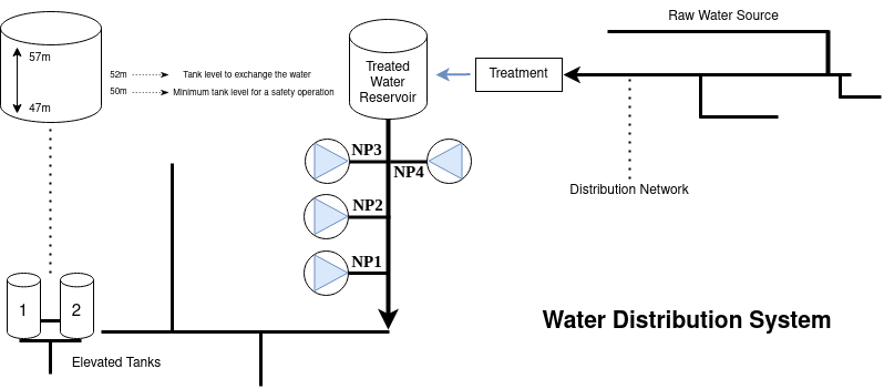
Figure 1: Water distribution system overview. The system has four pumps with fixed speed (ON/OFF) and two elevated tanks.

Figure 1 shows an overview of the water distribution system considered in this work. The system collects and treats the raw water from wells before storing it in a reservoir. In the water utility, four distribution pumps (NP1 to NP4) of different sizes are available for pumping the water through the system network into two storage tanks. The start/stop control operates the pumps. Speed or throttle control are not utilized. At most, only one pump can be running, and parallel operation is usually not applied. However, it is possible in case of exceptionally high water demand. A decision process has to decide on the operation of the most suitable pump regarding the water demand forecast, energy consumption, water quality, security of supply, and operational reliability. The tanks are located approximately 47m above the pump station. Both storage containers have identical dimensions and can be treated as a single tank with a storage volume of 16000m³. The maximum water level is 10m. Thus, the geodetic height between pumps and tank is [47, 57]m.

In the water distribution system, the human operation (behavioral policy) follows a strategy to handle the pump schedule. Figure 2 shows the effects of this behavioral policy. As shown in Figures 2, 2, 2, the operation fills the tank to a high level before the peak in water consumption (see Figures 2, 2, 2), and then they let it decrease along the day to provide water exchange and keep water’s quality. A safety operation must guarantee the tank level with at least 3m filled once it allows the system operators to handle unexpected situations. Figures 2, 2, 2, shows the average daily pump switch per month. Each pump switch is considered either ON to OFF or OFF to ON, counting +1. Thus, we could say that the current pump operation generally uses each pump at most once a day. Although it is difficult to measure the impact of a strategy in preserving the system’s assets, the idea is to minimize the amount of switching and provide a distribution pumps usage. Finally, in Figures 2, 2, 2 we show the electricity consumption where given the pumps settings, we can see the prioritization of the use of pump NP2.

3 A Partially Observable Markov Decision Process for the Pump Scheduling Problem

The RL problem statement can be formalized as a POMDP [8], defined by the tuple ($\mathcal{S}$, $\mathcal{A}$, $\mathcal{P}$, $\mathcal{R}$, $\Omega$, $\mathcal{O}$, $\gamma$), where:

• $\mathcal{S}$ is the state space;

• $\mathcal{A}$ is the action space;

• $\mathcal{P}:\mathcal{S}\times\mathcal{A}\times\mathcal{S}\mapsto[0,1]$ is the transition probability for being in some state $s\in\mathcal{S}$, perform an action $a\in\mathcal{A}$ and reach a state $s^{\prime}\in\mathcal{S}$

• $\mathcal{R}:\mathcal{S}\times\mathcal{A}\mapsto\mathbb{R}$ is the reward function;

• $\mathcal{O}:\mathcal{S}\times\mathcal{A}\times\Omega\mapsto[0,1]$ is the probability to receive an observation $o\in\Omega$ about the next state $s^{\prime}$ ;

• $\Omega$ denotes the observation space;

• $\gamma\in[0,1]$ is the discount factor that balances the relevance of immediate reward over rewards in the future;

The objective in the PO(MDP) is to learn a policy $\pi:S\mapsto A$ aiming maximize the expected discount rewards $J(\pi)=\mathbb{E}[\sum_{t=1}^{T}\gamma^{t}r(s_{t},a_{t})]$. In previous work [7], we cast the pump scheduling problem for a water system as an episodic POMDP. We consider the daily cycle pattern observed in the water consumption to define the episode length. Thus, each episode has a length of 1440 timesteps or one day of operation. The state/observation space and reward were partially based on data that sensors could gather, such as the tank level, water consumption, flow rate $Q$, and hydraulic head $H$. The action space $\mathcal{A}$ represents the discrete set of pumps (NP1 to NP4) and the option to turn all of them off (NOP). These pumps have different flow rates $Q$, which leads to distinct electricity consumption $kW$. Thus, the decision process consists of defining a policy that meets the water demand while limiting electricity consumption and satisfying safety constraints. Below, we review the state-action space and the proposed reward function.

State/Observation: The states/observation is represented by the $tank~{}level_{(t)}\in[47,57]$ and a given $water~{}consumption_{(t)}$ for a $time~{}of~{}day~{}(t)$, the respective $month$, the $action\in\mathcal{A}$ at $t-1$, the cumulative $time~{}running\in[0,1440]$ of pumps along with an episode, and a binary value called $water~{}quality$ that indicates if during the episode the $tank~{}level$ achieved a level lower than 53m.

The state’s representation is responsible for providing information to achieve the desired behavior through the reward function presented next. Thus, the features were selected aiming to:

• Provide information regarding the system’s current state, such as tank level and water consumption;

• Understand the cyclical behaviour of water consumption along the hours of the day in different seasons of the year;

• Lead the agent to avoid switching the pump operation as well as make a balance of their use;

• Provide information that could lead to preserving the water quality;

Action: The action space corresponds to the pumps available and the option to turn them off, such that $\mathcal{A}=\{$NP1, NP2, NP3, NP4, NPO$\}$. These pumps have different sizes which corresponds to distinct $Q$ and $kW$, being NP1 > NP2 > NP3 > NP4. The action NOP has $Q,kW=0$.

Reward function: We defined two dense reward functions through Eq. 1 and 2, where $P$ correspond to the cumulative time along an episode that some pump is running. These reward functions intends to balance the sub-goals: (i) enhance the efficiency of the pump operation; (ii) maintain safe levels of tank operation; (iii) penalize switches and provide distribution of the use of the pumps; (iv) maintain the water quality. We present in the Algorithms 1 and 2 how these reward are calculated.

Although we do not assume that these dense reward functions induce optimal policies, handcrafting them requires a considerable engineering burden [21]. To overcome this and address new challenges whenever the case, we suggest future research consider mimicking the behavioral policy assuming a goal-oriented approach. The goals, for instance, could be designed to meet certain tank levels by associating them with time windows, targeting the behavior observed in Figures 2 2 2.

$$r_{t}=e^{1/(-Q_{t}/kW_{t})}-B*\psi+\log(1/(P+\omega))$$ (1)

$$r_{t}=-e^{(-1/kW_{t})}-B*\psi+\log(1/(P+\omega))$$ (2)

Algorithm 1 Reward Function Eq. 1

$\psi\leftarrow 10$

if $action_{(t-1)}=action_{(t)}$ or $time~{}running(action_{(t)})=0$ or $action_{(t)}=$ NOP  then

     $\omega\leftarrow 1$

else

     $\omega\leftarrow 30$ $\triangleright$ Penalize pump switch

end if

if $tank~{}level_{(t)}>49$ and $tank~{}level_{(t)}<50$  then

     $B\leftarrow||tank~{}level_{(t)}-50||$

else if $tank~{}level_{(t)}\leq 49$ or $tank~{}level_{(t)}=57$ then

     $B\leftarrow 1$

else if $tank~{}level_{(t)}\geq 50$ and $tank~{}level_{(t)}<53$ and not $water~{}quality$ then

     $B\leftarrow-1$

else

     $B\leftarrow 0$

end if

if $action_{(t)}~{}\neq$ NOP then

     $r_{(t)}\leftarrow e^{(-Q_{t}/kW_{t})}-B\times\psi+\log(1/(time~{}running(action_{(t)}+\omega))$

else

     $r_{(t)}\leftarrow-B\times\psi+\log(1/(time~{}running(action_{(t)})+\omega))$

end if

Algorithm 2 Reward Function Eq. 2

$\psi\leftarrow 10$

if $action_{(t-1)}=action_{(t)}$ or $time~{}running(action_{(t)})=0$ then

     $\omega\leftarrow 1$

else

     $\omega\leftarrow 30$ $\triangleright$ Penalize action switch

end if

if $tank~{}level_{(t)}>49$ and $tank~{}level_{(t)}<50$ then

     $B\leftarrow||tank~{}level_{(t)}-50||$

else if $tank~{}level_{(t)}\leq 49$ or $tank~{}level_{(t)}=57$ then

     $B\leftarrow 1$

else if $tank~{}level_{(t)}\geq 50$ and $tank~{}level_{(t)}<53$ and not $water~{}quality$ then

     $B\leftarrow-1$

else

     $B\leftarrow 0$

end if

if $action_{(t)}~{}\neq~{}NOP$ then

     $r_{(t)}\leftarrow-e^{(-1/kW_{t})}-B\times\psi+\log(1/(time~{}running(action_{(t)})+\omega))$

else

     $r_{(t)}\leftarrow-B\times\psi+\log(1/(time~{}running(action_{(t)})+\omega))$

end if

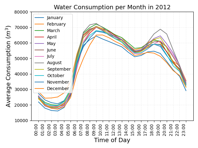
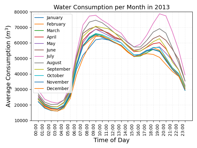
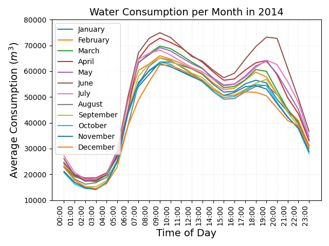
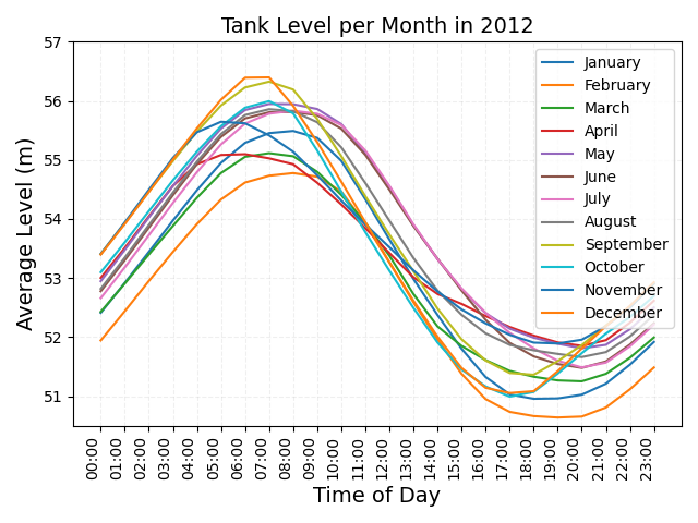
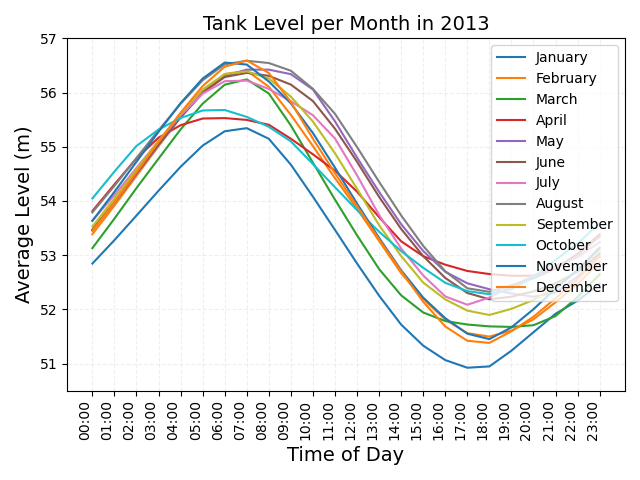
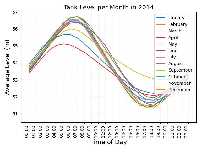
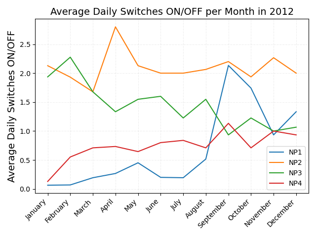
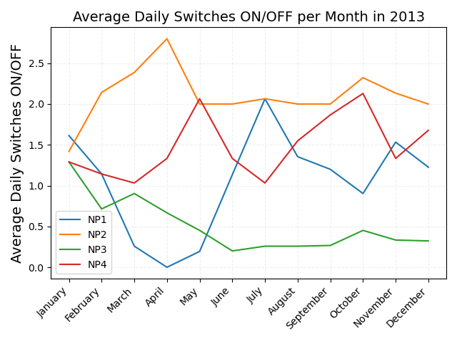
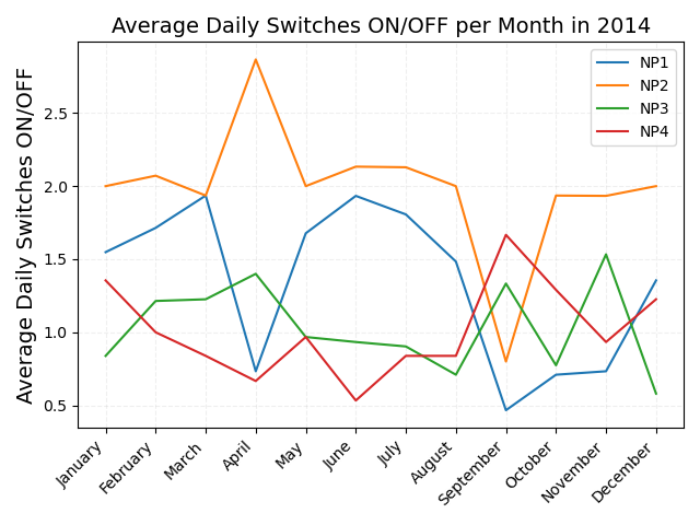
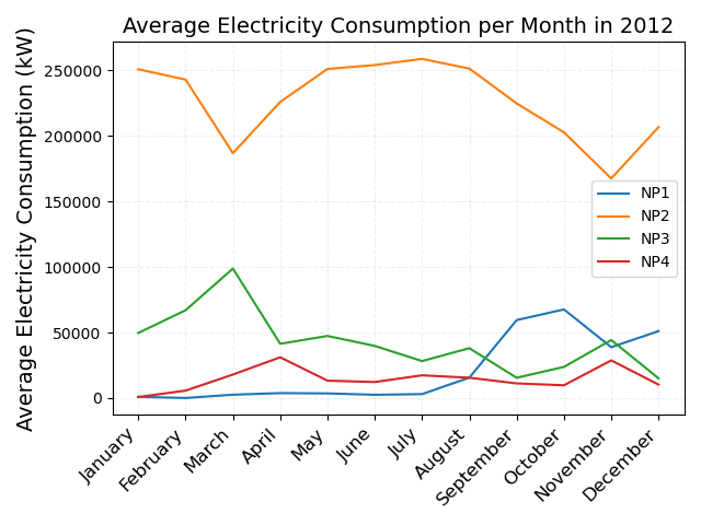
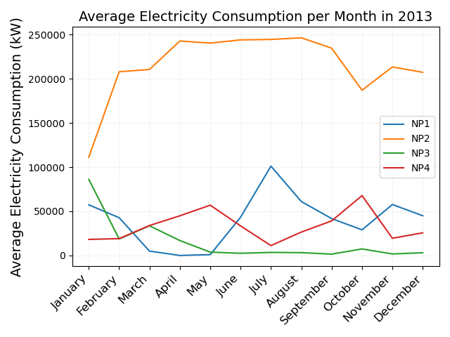
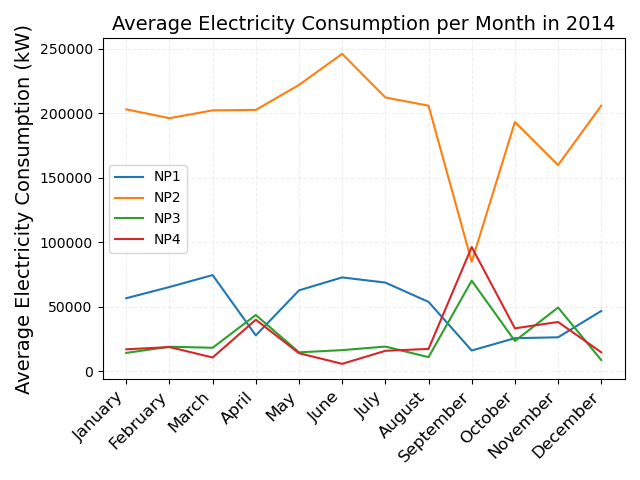
Figure 2: Overview of human operation for the water system. 2 2 2 show the water comsumption pattern. 2 2 2 show the tank level profile for the adopted strategy. 2 2 2 are the pump switch daily average and 2 2 2 are the average electricity consumption per month.

4 Casting the Water Distribution System Simulator into RL Settings

An RL agent, after applying an action $a$ in the state $s$, receives a reward $r$ and reaches a new state $s^{\prime}$, what is called transition $\tau=<s,a,r,s^{\prime}>$. Figure 3 presents how we model this dynamic for the pump scheduling problem using the simulator. First, real water consumption data at a given time $t$ is necessary as input to the simulator since it can not be generated through new interactions. After that, we need to define an initial condition for the tank level, among other features that compose the state $s$ representation. Given a state $s$, we can then apply an action to that state. In the codebase provided, we select the action looking at the real data, although any other policy could be used. A pump $p$ is ON if its value $kW_{p}(t)\neq 0$ in the dataset. If for all pumps $p$ the values $kW=0$, no pump is in operation, and the resulting action is NOP.

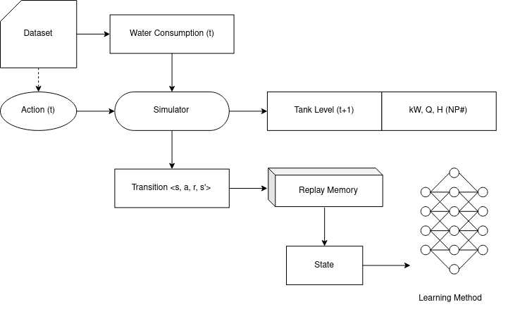
Figure 3: The dynamics of an MDP and the RL learning process through the water distribution system simulator.

Once an action $a$ is applied to the state $s$, the simulator outputs the values of $Q_{p}$, $kW_{p}$, and $H_{p}$ for the respective timestep $t$ (see details in  A.2). These values can then used to calculate a reward $r(t)$. Furthermore, a new tank level is observed at $t+1$, corresponding to state $s^{\prime}$. Thus we have a loop in which transitions are generated and stored in the Experience Replay [22], implemented with prioritization mechanism [23]. Finally, we can use these experiences to learn a new policy $\pi_{a}$, different from the behavioral policy $\pi_{b}$ which generated the dataset. To do so, we provide an implementation of Random Ensemble Mixture (REM) [24] as a learning algorithm. REM is dropout inspired convex combination of $K$ parametric Q-functions aiming to mitigate overestimation in offline RL settings. The underlying idea is for each policy update, generate a set of $k$ random weights $\alpha$ such that $Q(s,a)^{k}_{\theta}=\{\alpha_{1}Q(s,a)_{\theta_{1}}+\alpha_{2}Q(s,a)_{\theta_{2}}+\alpha_{3}Q(s,a)_{\theta_{3}}+...+\alpha_{k}Q(s,a)_{\theta_{k}}\}$ and $\sum_{k}\alpha_{k}=1$.

5 Addressing Challenges

This section lists some challenges that can be addressed using the simulator/dataset.

Modeling the problem. The pump scheduling problem does not have a prior state representation or a single specified reward function. For this reason, state representation learning [25, 26, 27] can explore more informative and low dimensional state representations for efficient policy learning. The same applies to reward engineering. Specifying a reward function is difficult once it must encapsulate and balance multiple goals that might be contradictory. A way to overcome this is through inverse RL [28] approaches to extract a reward function from the demonstrations. Moreover, we presented a suggestion to model the problem as a goal/task-oriented with sparse rewards to allow the evaluation of approaches [20] that deal with the lack of reward signals.

Reset mechanism. We have modeled the pump scheduling as an episodic POMDP where the agent interacts for a limited number of timesteps. Therefore, our configuration is reset-free, which means no mechanism is applied to start an episode under a known distribution of initial states. In other words, it means that the last step of an episode is the initial one for the next episode. Thus, a suitable policy must be robust to handle the variability of initial conditions, providing dynamism challenge [29].

An exploration challenge. One of the constraints set for controlling the system is to avoid switching the pump operation too frequently to protect the assets. Thus, exhaustive exploration strategies such as epsilon-greedy [8] are contradictory to the idea of performing the same action selection over many timesteps and may prematurely converge to suboptimal policies. Furthermore, approaches that attempt to cover unknown areas of state space can lead to meaningless states that do not meet the safety constraints. Thus, the pump scheduling problem can be a setting for evaluating exploration strategies that aim to enhance sample efficiency or limit state visitation to those that meet system safety constraints [30].

Learning from demonstrations. Some real-world settings may restrict the learning process to logged data. This constraint is due to the difficulty of creating accurate simulators or even safety constraints. For example, an autonomous vehicle cannot learn by interacting with the environment through trial-error, both for safety and cost reasons. For this, offline RL [17] approaches such as BCQ [31, 32], REM [24], Conservative Q-learning [33], and Averaged-DQN [34] were designed to increase the efficiency of exploiting previously collected data, mainly tackling the overestimation phenomena [35]. This data can be, for instance, obtained by human operation in the real-world system, as in the present case. In [7], we show that a large dataset is capable of producing policies through offline approaches that can outperform the behavioral policy. Thus, the present dataset can serve as a benchmark for offline RL approaches. Finally, these expert demonstrations can guide the agent’s actions through imitation learning [36], used to build models [37, 38], or boost the learning process [11].

Continuous action-space. The set of actions of the water distribution system is discrete. There is a finite set of pumps that operate with a fixed speed beside the option to turn all of them off. Although not explored in previous works, the simulator can adapt to variable speed pump(s). Then, approaches suitable for continuous action space, such as actor-critic [8], can be evaluated while exploring the environment.

6 Related Works

We discuss in this section some related approaches found in the literature regarding applied RL to control and pump scheduling optimization.

Control using Reinforcement Learning. In [39] the authors use Deep Recurrent Q-Networks [40] in the scenario of a smart grid. The objective is to develop a pricing strategy to maximize broker’s (agents) profits. It is proposed a reward shaping strategy once customers are clustered according to their consumption patterns and managed by their respective sub-brokers. Then, a mechanism for credit assignment was necessary to indicate the contribution of each sub-broker to the global return. Wei and colleagues [41] proposes a data-driven solution to control HVAC (heating, ventilation and air conditioning) system. The objective is to control the environment temperature by handling numerous disturbances with real-time data. The possible actions are a discrete set of airflow rates divided by building zone. Then, the approach split each zone controlling it by distinct artificial neural networks. Sivakumar et al. [42] propose a network control strategy that acts asynchronously with the environment. The delay, which authors call by $\delta$, corresponds to the policy lookup time when selecting an action. Meanwhile, the network proceeds transmitting data in the interval [t, t + $\delta$]. Thus, the transitions are not only dependent on the state and action at some timestep $t$ but also the previous action at $t-1$. In [43] the problem of congestion control in networks is also addressed, and a testbed was released. In [44], the authors applied RL to a flight controller of a stratospheric balloon which must handle a partially observable environment and continuous interaction. Finally, Degrave et al. [45] use RL for nuclear fusion control, which achieved a variety of plasma configurations.

Pump Scheduling. In [4], the authors adopted a branch-and-bound algorithm that interacts with the hydraulic simulator EPANET  to evaluate decisions at each timestep corresponding to 1 hour in a horizon length of 24 hours. The proposed algorithm aims to find a solution with minimum electricity consumption. Menke and colleagues in [6] also used a branch-and-bound approach through an algorithm with several steps for the branching procedure. The objective function adopted has contact with the presented in this work. The authors consider pumps with fixed speed (ON/OFF), intending to minimize the electricity consumption meanwhile penalizing switches in the pump operation. In [46], the authors also applied DRL to control a real-world scenario of a wastewater treatment plant. Differently from our study case, in their system, the electricity price has different tariffs throughout the day, which add one more constraint to the proposed strategy.

This section presents some control-related scenarios where the approach used was RL-based. Indeed, RL has already shown remarkable success in applications such as games and is beginning to show potential for sensitive real-world applications such as nuclear fusion. Afterward, we discuss some approaches for the specific scenario of pump scheduling. We believe that a data-driven solution based on RL can overcome some limitations presented in previous works, such as robustness and scalability. This work distinguishes itself from the others by releasing a testbed aiming RL approaches for the pump scheduling problem.

7 Conclusion

We release a testbed for RL where logged data and a water distribution system simulator are available. This data was gathered through sensors in the real-world operation controlled by humans and the simulator validated by hydraulic specialists. Later, we present some statistics on the real-world water supply and cast the pump scheduling problem in the RL settings. To that end, we proposed POMDP for the problem, with the state-action space representation and the reward function. We combine this representation in the simulator, providing an end-to-end process to learn new policies from the logged data. Finally, we list some challenges that could be addressed in future works using the tools and data that have been made available. Thus, we hope to facilitate research and bridge the gap between RL and real-world applications.

Appendix A Appendix

A.1 Electricity consumption (kW) using the simulator

Figure 4 shows the electricity consumption of the measured (real world) data and the simulator. Note that the range of values between the measured and simulated data differ. The reason is due to not taking into account the pump efficiency in Equation 3. Thus, we obtain the values for measured data by taking the hydraulic power ($P_{h}$), and dividing it by the efficiency $\eta$:

$$P_{h}(kW)=Q\rho gh/(3.6~{}10^{6}),\textrm{where}$$ (3)

• $Q$ is the flow $(m^{3}/h)$

• $\rho$ is the density of fluid $(kg/m^{3})$

• $g$ is the acceleration of gravity $(9.81m/s^{2})$

• $h$ is the differential head (m)

Figure 4: Average electricity consumption calculated using measured data 4 and simulator 4.

A.2 The simulator program

The simulator was developed for investigating the operating behavior of distribution pumps in a real water network in Germany. The calculation of the operating point of a pump is based on intersecting the characteristic curve of a pump (hydraulic head vs. flow rate) with the system curve.

The system curve describes the amount of pressure or hydraulic head which is necessary to deliver a certain flow into a system. For the system curve one can distinguish between a static and a dynamic part (Figure 5). The static part is independent of the flow rate caused by a difference in geodetic height, e.g. when liquid is pumped into an elevated storage tank, or by a static pressure difference. The dynamic part is caused by hydraulic losses in the piping system and increase with the second power of the flow rate. The operating point of the pump is the intersection of the system curve and the hydraulic head curve of the pump.

For the water system according to Figure 1 the system curve is not constant. The static part depends on the current tank level and to a smaller amount on the water demand. The slope of the system curve depends on the hydraulic losses in the piping system and in case of a water system of the current water demand. For a high water demand, the pressure in the system is smaller and therefore the slope of the system curves becomes smaller, too. In cases of a small water demand, the slope is greater, because of the higher pressure in the system. Based on measurements, the relationship of tank level, water demand static head and slope of the system curve were derived.

With the simulator the pump operation of an arbitrary time period can be calculated. At the beginning, the expected water demand has to be defined for each time step. Also, the initial tank level and the pump schedule have to be specified. For the simulation, the current system curve is calculated based on current tank level and water demand. At each time step it is checked whether a pump is in operation. If this is the case, the operating point of the pump is calculated by intersecting the pump curve with the system curve. In case the flow rate of the pump is larger than the water demand, the tank level is increased accordingly. On the contrary, when the flow rate is smaller than the water demand, the tank level is decreased. With the new tank level and the water demand of the next time step, a new system curve is calculated for the next time step. This procedure is continued in a loop for the specified time period.

A.3 Extending the simulator for applying speed control to pumps

Speed control is an efficient method for controlling the operating point of a pump. In this case, the frequency of the motor is changed by a frequency converter. By the change in speed, the characteristic curves of the pump for hydraulic head vs. flow rate and efficiency vs. flow rate are changed. The change in flow rate and hydraulic head can be calculated by means of the affinity laws (4 and 5) where the flow rate (Q) changes proportional with the speed (n) and the hydraulic head (H) changes proportional to the second power of the speed.

$$Q\propto n$$ (4)

$$H\propto n^{2}$$ (5)

With equations 4 and 5 it can be shown that the hydraulic head changes with the second power of the flow rate (6) where $Q_{1}$ and $H_{1}$ are flow rate and hydraulic head on the pump curve for the initial speed.

$$H_{x}=\left(\frac{H_{1}}{Q_{1}^{2}}\right)*Q_{x}^{2}$$ (6)

So, all points of a pump curve are moved on quadratic curves through the origin of the diagram (Figure 5).

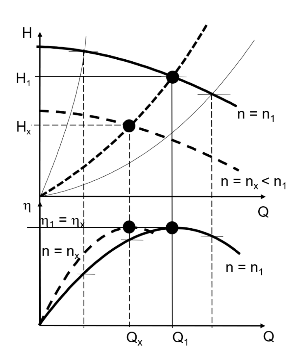
Figure 5: Influence of speed control on pump curve 5 [47] and relationship of pump curve and system curve 5.

Changing the speed, the efficiency curve is also modified. In case the point on the efficiency curve is identical to the point of best efficiency, it will also be the point of best efficiency at any other speed. All other points on the efficiency curve are shifted on a quadratic curve and maintain their position relative to the point of best efficiency. The maximum value of the efficiency remains nearly constant. Effects of the change in Reynolds-number can be included by empirical equations according to Ackeret [48] for example:

$$\frac{\left(1-\eta_{1,opt}\right)}{\left(1-\eta_{2,opt}\right)}=\left(1-V\right)+V*\left(\frac{Re_{2}}{Re_{1}}\right)^{(\frac{1}{\alpha})}$$ (7)

The change in operating point of the pump depends on the shape of the system curve. For systems where the static part is zero, the system curve is identical to the affinity parabola. In this case it is possible that a pump is always operating at the point of best efficiency when the speed is changed. Figure 6 shows the situation for a non-zero static part. In this case, the intersection of pump curve and system curve is not a point on the parabola based on the affinity laws and the pump is operating with a smaller efficiency under part-load conditions when the speed is reduced.

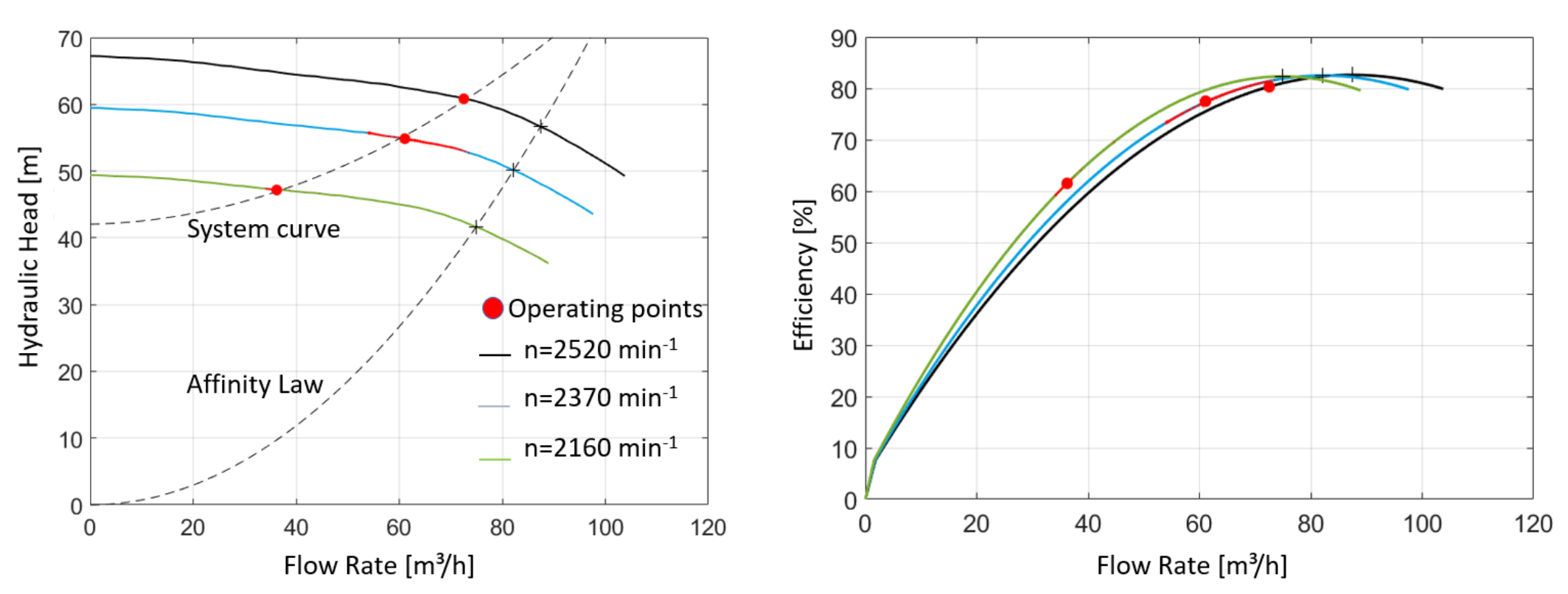
Figure 6: Influence of speed control on operating point.

The function for speed control can be included in the main code of the simulator. With this function it is possible to calculate the pump curve every time the speed has changed.

References

- [1] Antonio Candelieri, Raffaele Perego, and Francesco Archetti. Bayesian optimization of pump operations in water distribution systems. Journal of Global Optimization, 71(1):213–235, 2018.
- [2] Sanda-Carmen Georgescu and Andrei-Mugur Georgescu. Pumping station scheduling for water distribution networks in epanet. UPB Sci. Bull, Series D, 77(2):235–246, 2015.
- [3] Tiago Luna, João Ribau, David Figueiredo, and Rita Alves. Improving energy efficiency in water supply systems with pump scheduling optimization. Journal of cleaner production, 213:342–356, 2019.
- [4] Luis Henrique Magalhães Costa, Bruno de Athayde Prata, Helena M Ramos, and Marco Aurélio Holanda de Castro. A branch-and-bound algorithm for optimal pump scheduling in water distribution networks. Water resources management, 30(3):1037–1052, 2016.
- [5] Folorunso Taliha Abiodun and Fatimah Sham Ismail. Pump scheduling optimization model for water supply system using awga. In 2013 IEEE Symposium on Computers Informatics (ISCI), pages 12–17, 2013.
- [6] Ruben Menke, Edo Abraham, Panos Parpas, and Ivan Stoianov. Exploring optimal pump scheduling in water distribution networks with branch and bound methods. Water Resources Management, 30(14):5333–5349, 2016.
- [7] Henrique Donâncio and Laurent Vercouter. Safety through intrinsically motivated imitation learning. In Proceedings of the Adaptive and Learning Agents Workshop (ALA 2022), 2022.
- [8] Richard S. Sutton and Andrew G. Barto. Reinforcement Learning: An Introduction. A Bradford Book, Cambridge, MA, USA, 2018.
- [9] Haochen Liu, Zhiyu Huang, and Chen Lv. Improved deep reinforcement learning with expert demonstrations for urban autonomous driving. CoRR, abs/2102.09243, 2021.
- [10] Shixiang Gu, Ethan Holly, Timothy Lillicrap, and Sergey Levine. Deep reinforcement learning for robotic manipulation with asynchronous off-policy updates. In 2017 IEEE International Conference on Robotics and Automation (ICRA), page 3389–3396. IEEE Press, 2017.
- [11] Ashvin Nair, Bob McGrew, Marcin Andrychowicz, Wojciech Zaremba, and Pieter Abbeel. Overcoming exploration in reinforcement learning with demonstrations. In 2018 IEEE International Conference on Robotics and Automation (ICRA), pages 6292–6299, 2018.
- [12] Guillaume Lample and Devendra Singh Chaplot. Playing fps games with deep reinforcement learning. In Proceedings of the Thirty-First AAAI Conference on Artificial Intelligence, AAAI’17, page 2140–2146. AAAI Press, 2017.
- [13] Volodymyr Mnih, Koray Kavukcuoglu, David Silver, Alex Graves, Ioannis Antonoglou, Daan Wierstra, and Martin A. Riedmiller. Playing atari with deep reinforcement learning. CoRR, abs/1312.5602, 2013.
- [14] Peter R Wurman, Samuel Barrett, Kenta Kawamoto, James MacGlashan, Kaushik Subramanian, Thomas J Walsh, Roberto Capobianco, Alisa Devlic, Franziska Eckert, Florian Fuchs, et al. Outracing champion gran turismo drivers with deep reinforcement learning. Nature, 602(7896):223–228, 2022.
- [15] Oriol Vinyals, Igor Babuschkin, Wojciech M Czarnecki, Michaël Mathieu, Andrew Dudzik, Junyoung Chung, David H Choi, Richard Powell, Timo Ewalds, Petko Georgiev, et al. Grandmaster level in starcraft ii using multi-agent reinforcement learning. Nature, 575(7782):350–354, 2019.
- [16] Natasha Jaques, Asma Ghandeharioun, Judy Hanwen Shen, Craig Ferguson, Àgata Lapedriza, Noah Jones, Shixiang Gu, and Rosalind W. Picard. Way off-policy batch deep reinforcement learning of implicit human preferences in dialog. CoRR, abs/1907.00456, 2019.
- [17] Sergey Levine, Aviral Kumar, George Tucker, and Justin Fu. Offline reinforcement learning: Tutorial, review, and perspectives on open problems. CoRR, abs/2005.01643, 2020.
- [18] Marlos C. Machado, Marc G. Bellemare, Erik Talvitie, Joel Veness, Matthew J. Hausknecht, and Michael Bowling. Revisiting the arcade learning environment: Evaluation protocols and open problems for general agents. J. Artif. Intell. Res., 61:523–562, 2018.
- [19] Yuval Tassa, Yotam Doron, Alistair Muldal, Tom Erez, Yazhe Li, Diego de Las Casas, David Budden, Abbas Abdolmaleki, Josh Merel, Andrew Lefrancq, Timothy P. Lillicrap, and Martin A. Riedmiller. Deepmind control suite. CoRR, abs/1801.00690, 2018.
- [20] Marcin Andrychowicz, Filip Wolski, Alex Ray, Jonas Schneider, Rachel Fong, Peter Welinder, Bob McGrew, Josh Tobin, OpenAI Pieter Abbeel, and Wojciech Zaremba. Hindsight experience replay. In I. Guyon, U. V. Luxburg, S. Bengio, H. Wallach, R. Fergus, S. Vishwanathan, and R. Garnett, editors, Advances in Neural Information Processing Systems, volume 30. Curran Associates, Inc., 2017.
- [21] Conor F. Hayes, Roxana Radulescu, Eugenio Bargiacchi, Johan Källström, Matthew Macfarlane, Mathieu Reymond, Timothy Verstraeten, Luisa M. Zintgraf, Richard Dazeley, Fredrik Heintz, Enda Howley, Athirai A. Irissappane, Patrick Mannion, Ann Nowé, Gabriel de Oliveira Ramos, Marcello Restelli, Peter Vamplew, and Diederik M. Roijers. A practical guide to multi-objective reinforcement learning and planning. CoRR, abs/2103.09568, 2021.
- [22] Long Ji Lin. Self-improving reactive agents based on reinforcement learning, planning and teaching. Mach. Learn., 8:293–321, 1992.
- [23] Tom Schaul, John Quan, Ioannis Antonoglou, and David Silver. Prioritized experience replay. In 4th International Conference on Learning Representations, ICLR 2016, 2016.
- [24] Rishabh Agarwal, Dale Schuurmans, and Mohammad Norouzi. An optimistic perspective on offline reinforcement learning. In Hal Daumé III and Aarti Singh, editors, Proceedings of the 37th International Conference on Machine Learning, volume 119 of Proceedings of Machine Learning Research, pages 104–114. PMLR, 13–18 Jul 2020.
- [25] Timothée Lesort, Natalia Díaz Rodríguez, Jean-François Goudou, and David Filliat. State representation learning for control: An overview. CoRR, abs/1802.04181, 2018.
- [26] Changmin Yu, Dong Li, Jianye HAO, Jun Wang, and Neil Burgess. Learning state representations via retracing in reinforcement learning. In 10th International Conference on Learning Representations, ICLR 2022, 2022.
- [27] Astrid Merckling, Alexandre Coninx, Loic Cressot, Stephane Doncieux, and Nicolas Perrin. State representation learning from demonstration. In Machine Learning, Optimization, and Data Science, pages 304–315, Cham, 2020. Springer International Publishing.
- [28] Pieter Abbeel and Andrew Y. Ng. Apprenticeship learning via inverse reinforcement learning. In Proceedings of the twenty-first international conference on Machine learning, ICML ’04, New York, NY, USA, 2004. Association for Computing Machinery.
- [29] John D. Co-Reyes, Suvansh Sanjeev, Glen Berseth, Abhishek Gupta, and Sergey Levine. Ecological reinforcement learning. CoRR, abs/2006.12478, 2020.
- [30] Javier García and Fernando Fernández. A comprehensive survey on safe reinforcement learning. Journal of Machine Learning Research, 16(42):1437–1480, 2015.
- [31] Scott Fujimoto, Edoardo Conti, Mohammad Ghavamzadeh, and Joelle Pineau. Benchmarking batch deep reinforcement learning algorithms. arXiv preprint arXiv:1910.01708, 2019.
- [32] Scott Fujimoto, David Meger, and Doina Precup. Off-policy deep reinforcement learning without exploration. In Kamalika Chaudhuri and Ruslan Salakhutdinov, editors, Proceedings of the 36th International Conference on Machine Learning, volume 97 of Proceedings of Machine Learning Research, pages 2052–2062. PMLR, 09–15 Jun 2019.
- [33] Aviral Kumar, Aurick Zhou, George Tucker, and Sergey Levine. Conservative q-learning for offline reinforcement learning. In H. Larochelle, M. Ranzato, R. Hadsell, M.F. Balcan, and H. Lin, editors, Advances in Neural Information Processing Systems, volume 33, pages 1179–1191. Curran Associates, Inc., 2020.
- [34] Oron Anschel, Nir Baram, and Nahum Shimkin. Averaged-dqn: Variance reduction and stabilization for deep reinforcement learning. In Proceedings of the 34th International Conference on Machine Learning - Volume 70, ICML’17, page 176–185. JMLR.org, 2017.
- [35] Georg Ostrovski, Pablo Samuel Castro, and Will Dabney. The difficulty of passive learning in deep reinforcement learning. In Advances in Neural Information Processing Systems, volume 34, 2021.
- [36] Ahmed Hussein, Mohamed Medhat Gaber, Eyad Elyan, and Chrisina Jayne. Imitation learning: A survey of learning methods. ACM Comput. Surv., 50(2), apr 2017.
- [37] Tianhe Yu, Garrett Thomas, Lantao Yu, Stefano Ermon, James Y Zou, Sergey Levine, Chelsea Finn, and Tengyu Ma. Mopo: Model-based offline policy optimization. In H. Larochelle, M. Ranzato, R. Hadsell, M. F. Balcan, and H. Lin, editors, Advances in Neural Information Processing Systems, volume 33, pages 14129–14142. Curran Associates, Inc., 2020.
- [38] Rahul Kidambi, Aravind Rajeswaran, Praneeth Netrapalli, and Thorsten Joachims. Morel: Model-based offline reinforcement learning. In H. Larochelle, M. Ranzato, R. Hadsell, M. F. Balcan, and H. Lin, editors, Advances in Neural Information Processing Systems, volume 33, pages 21810–21823. Curran Associates, Inc., 2020.
- [39] Yaodong Yang, Jianye Hao, Mingyang Sun, Zan Wang, Changjie Fan, and Goran Strbac. Recurrent deep multiagent q-learning for autonomous brokers in smart grid. In Proceedings of the Twenty-Seventh International Joint Conference on Artificial Intelligence, IJCAI-18, pages 569–575. International Joint Conferences on Artificial Intelligence Organization, 7 2018.
- [40] Matthew Hausknecht and Peter Stone. Deep recurrent q-learning for partially observable mdps. In AAAI Fall Symposium on Sequential Decision Making for Intelligent Agents (AAAI-SDMIA15), November 2015.
- [41] Tianshu Wei, Yanzhi Wang, and Qi Zhu. Deep reinforcement learning for building hvac control. In Proceedings of the 54th Annual Design Automation Conference 2017, DAC ’17, New York, NY, USA, 2017. Association for Computing Machinery.
- [42] Viswanath Sivakumar, Tim Rocktäschel, Alexander H. Miller, Heinrich Küttler, Nantas Nardelli, Mike Rabbat, Joelle Pineau, and Sebastian Riedel. MVFST-RL: an asynchronous RL framework for congestion control with delayed actions. CoRR, abs/1910.04054, 2019.
- [43] Nathan Jay, Noga Rotman, Brighten Godfrey, Michael Schapira, and Aviv Tamar. A deep reinforcement learning perspective on internet congestion control. In Kamalika Chaudhuri and Ruslan Salakhutdinov, editors, Proceedings of the 36th International Conference on Machine Learning, volume 97 of Proceedings of Machine Learning Research, pages 3050–3059. PMLR, 09–15 Jun 2019.
- [44] Marc G Bellemare, Salvatore Candido, Pablo Samuel Castro, Jun Gong, Marlos C Machado, Subhodeep Moitra, Sameera S Ponda, and Ziyu Wang. Autonomous navigation of stratospheric balloons using reinforcement learning. Nature, 588(7836):77–82, 2020.
- [45] Jonas Degrave, Federico Felici, Jonas Buchli, Michael Neunert, Brendan Tracey, Francesco Carpanese, Timo Ewalds, Roland Hafner, Abbas Abdolmaleki, Diego de Las Casas, et al. Magnetic control of tokamak plasmas through deep reinforcement learning. Nature, 602(7897):414–419, 2022.
- [46] Giup Seo, Seungwook Yoon, Myungsun Kim, Changho Mun, and Euiseok Hwang. Deep reinforcement learning-based smart joint control scheme for on/off pumping systems in wastewater treatment plants. IEEE Access, 9:95360–95371, 2021.
- [47] Hellmann Dieter-Heinz. Lecture Notes on Centrifugal Pumps and Compressors. Technical University of Kaiserslautern, 2004.
- [48] Carl Pfleiderer and Hartwig Petermann. Strömungsmaschinen. Springer-Verlag Berlin Heidelberg, 2005.